A measurement campaign to assess sources of error in microwave link rainfall estimation

We present a measurement campaign to address several error sources associated with rainfall estimates from microwave links in cellular communication networks. The core of the experiment is provided by three co-located microwave links installed between two major buildings on opposite sides of the small town of Wageningen, approximately 2 km apart: a 38 GHz formerly commercial microwave link, as well as 26 and 38 GHz (dual-polarization) research microwave links. Transmitting and receiving antennas have been attached to masts installed on the roofs of the two buildings, about 30 m above the ground. This setup was complemented with an infrared large-aperture scintillometer, installed over the same path, as well as five laser disdrometers positioned at several locations along the path and an automated rain gauge. Temporal sampling of the received signals was performed at a rate of 20 Hz. The setup was monitored by time-lapse cameras to assess the state of the antennas as well as the atmosphere. The experiment was active between August 2014 and December 2015. Data from an existing automated weather station situated just outside Wageningen was further used to compare and to interpret the findings. In addition to presenting the experiment, we also conduct a preliminary global analysis and show several cases highlighting the different phenomena affecting received signal levels: rainfall, solid precipitation, temperature, fog, antenna wetting due to rain or dew, and clutter. We also briefly explore cases where several phenomena play a role. A rainfall intensity (R) – specific attenuation (k) relationship was derived from the disdrometer data. We find that a basic rainfall retrieval algorithm without corrections already provides a reasonable correlation to rainfall as measured by the disdrometers. However, there are strong systematic overestimations (factors of 1.2–2.1) which cannot be attributed to the R–k relationship. We observe attenuations in the order of 3 dB due to antenna wetting under fog or dew conditions. We also observe fluctuations of a similar magnitude related to changes in temperature. The response of different makes of microwave antennas to many of these phenomena is significantly different even under the exact same operating conditions and configurations.

1 Introduction

Accurate and real-time precipitation measurements are important for flood prediction, especially in urban areas. Traditional measurement techniques such as rain gauges have an insufficient temporal and spatial network density to allow for accurate measurements in an urban setting (Schilling, 1991; Berne et al., 2004). Furthermore, their spatial representativeness is limited because of their small sampling areas, making them essentially zero-dimensional point measurements. Weather radars, in contrast, have a much larger sampling area and provide full coverage making their observations more representative of the spatial precipitation distribution, but their space-time resolution is often limited, in particular for urban applications. Furthermore, radar observations take place higher up in the atmosphere the further away they are from the radar antenna (typical observation heights can be more than 1000 m). Therefore, their measurements may not be representative of the situation near ground level. Finally, their high cost may be prohibitive for use by developing countries or local authorities.

Microwave link measurements may be a promising addition to the existing range of rain measurement techniques. The use of such instruments for measuring rainfall was first suggested by Atlas and Ulbrich (1977). With respect to spatial representativeness and resolution, microwave links can fill some of the gaps between rain gauges and weather radar. The area sampled is along the path of the link: typically about a few kilometres long and a few metres to dozens of metres wide at the widest point. This makes the sampling footprint approximately one-dimensional. This is more spatially representative than a rain gauge, but less so than radar. However, microwave links have two major advantages over radar: they measure much closer to the ground than radar (typically a few tens of metres), and the relation between the measured variable (specific attenuation in the case of links and radar reflectivity in the case of traditional radar) and rainfall intensity is much better defined and closer to linear for microwave links. Despite these advantages, microwave links had not been deployed at a large scale for the purpose of rainfall monitoring, for the cost of setting up such a network would still have been quite severe. The real potential of microwave link measurements for rainfall measurement came with the realization that the microwave links used in cellular communications networks could be repurposed as rainfall measurement devices, which was demonstrated by Messer et al. (2006) and Leijnse et al. (2007a). Doing so eliminates most of the cost of this technique as existing infrastructure can be used. This is especially valuable in developing countries, which typically have few rain gauges let alone weather radar, yet often do have an extensive mobile phone network (Doumounia et al., 2014). In the recent past there have been a number of studies about the application of commercial microwave link networks for rainfall measurements. These studies have demonstrated the feasibility of this method in southern Germany (Chwala et al., 2012), the Netherlands (Overeem et al., 2011, 2013), Israel (Zinevich et al., 2008, 2009) and also in Burkina Faso (Doumounia et al., 2014) and Brazil (Rios Gaona et al., 2018).

Although the rainfall maps produced by this method show surprisingly good correspondence with the gauge-adjusted radar product (Overeem et al., 2013), there are still inaccuracies remaining in the final products (Leijnse et al., 2008, 2010; Zinevich et al., 2010). Error sources can generally be divided into errors due to the mapping of the rainfall estimates from the microwave links, and errors in the individual measurements and the rainfall retrieval algorithm. It is in this last category where the largest remaining sources of error reside and not in the mapping (Rios Gaona et al., 2015). Therefore, further research is needed regarding the physical aspects of the attenuation measurements themselves. Several possible sources of error affecting the quality of rainfall retrievals from single microwave links have been identified previously: the wet antenna effect and related dew formation on antennas (Minda and Nakamura, 2005; Leijnse et al., 2008; Schleiss et al., 2013), humidity (Holt et al., 2003) and temperature (Minda and Nakamura, 2005), solid precipitation, and spatial variability of rainfall (Berne and Uijlenhoet, 2007). Opportunities for simultaneous measurement of environmental variables other than rainfall have also been identified, such as evaporation (Leijnse et al., 2007b), fog (Liebe et al., 1989; David et al., 2013), humidity (Chwala et al., 2014), and hydrometeor type (Cherkassky et al., 2014).

In this paper we describe a dedicated microwave link experiment that has been set up in the college town of Wageningen and present an analysis of the results. The field experiment was designed to provide validation data for microwave link rainfall retrieval at the scale of a single link, and to be able to compare different types of links simultaneously measuring along the same path. The goal of the analysis is to give a comprehensive overview of the phenomena encountered by a typical microwave link and to evaluate their relevance to a rainfall intensity retrieval. In order to do so we employ a relatively straightforward retrieval algorithm with a minimum number of corrections and make use of a number of auxiliary measurement devices to gain insight into the retrieved signal. In Sect. 2, a brief overview of the theoretical background pertaining to the operating principles of microwave link rainfall measurements is given. Section 3 covers a description of the experimental setup and the employed instruments. In Sect. 4, the data processing methods applied in this experiment are detailed. In Sect. 5, the obtained experimental data are presented and an inventory of encountered phenomena is given. Finally, in Sect. 6 conclusions are drawn.

2 Theoretical background

Both the attenuation of a microwave signal by rain drops during a rain event and the corresponding rainfall intensity can be related to the rain drop size distribution. The rainfall intensity (in mm h⁻¹) can be calculated as follows, assuming the density of water to be constant:

$$\begin{array}{}\text{(1)}& R\left(t\right)=C_{\mathrm{R}}\underset{\mathrm{0}}{\overset{\mathrm{\infty }}{\int }}V\left(D\right)v\left(D\right)N\left(D,t\right)\mathrm{d}D.\end{array}$$

Here V(D) is the volume of a raindrop in mm³, D is the raindrop diameter in mm, v(D) is the fall velocity (in m s⁻¹) of a particle with diameter D and N(D,t) is the density of particles with diameter D per m³ or drop size distribution (DSD) as a function of time t and $R_{\mathrm{C}}=\mathrm{3.6}\times {\mathrm{10}}^{-\mathrm{3}}$ is a unit conversion factor. When dividing the particle diameter into discrete classes (as is measured by a disdrometer) this can be approximated as follows:

$$\begin{array}{ll}\text{(2)}& {\displaystyle }& {\displaystyle }R\left(t\right)=C_{\mathrm{R}}{\displaystyle \frac{\mathrm{1}}{\mathrm{6}}}\mathit{\pi }\underset{\mathrm{0}}{\overset{\mathrm{\infty }}{\int }}{D}^{\mathrm{3}}v\left(D\right)N\left(D,t\right)\mathrm{d}D{\displaystyle }& {\displaystyle }\approx C_{\mathrm{R}}{\displaystyle \frac{\mathrm{1}}{\mathrm{6}}}\mathit{\pi }{\sum }_{i=\mathrm{1}}^n{D}_i^{\mathrm{3}}v\left(D_i\right)N\left(D_i,t\right)\mathrm{\Delta }{D}_i.\end{array}$$

Here, D_i is the mean diameter of the i-th drop size class, N(D_i,t) is the discrete drop size distribution. ΔD_i is the width of the i-th diameter class, and n is the number of drop size classes. A similar function defines the specific (logarithmic) attenuation (in dB km⁻¹), where we assume that the particle density is low enough such that multiple scattering can be neglected:

$$\begin{array}{ll}\text{(3)}& {\displaystyle }& {\displaystyle }k\left(t\right)=C_k\underset{\mathrm{0}}{\overset{\mathrm{\infty }}{\int }}{\mathit{\sigma }}_{\mathrm{ext}}\left(D\right)N\left(D,t\right)\mathrm{d}D{\displaystyle }& {\displaystyle }\approx C_k{\sum }_{i=\mathrm{1}}^n{\mathit{\sigma }}_{\mathrm{ext}}\left(D_i\right)N\left(D_i,t\right)\mathrm{\Delta }{D}_i.\end{array}$$

Here, σ_ext(D) (in mm²) is the extinction cross-section of a hydrometeor with a diameter D and $C_k=\mathrm{100}\cdot \ln {\left(\mathrm{10}\right)}^{-\mathrm{1}}$ is a unit conversion factor. σ_ext(D) is also dependent on the frequency and polarization of the incident radiation. It can be derived from the forward scattering amplitude matrix S(D), which relates the incoming electromagnetic wave with the outgoing (forward scattered) wave,

$$\begin{array}{}\text{(4a)}& \left(\begin{array}{l}{E}_{\mathrm{h}}\\ E_{\mathrm{v}}\end{array}\right)=\mathbf{S}\left(D\right)\left(\begin{array}{l}{E}_{\mathrm{h}\mathrm{0}}\\ E_{\mathrm{v}\mathrm{0}}\end{array}\right)=\left(\begin{array}{ll}{S}_{\mathrm{hh}}\left(D\right)& S_{\mathrm{hv}}\left(D\right)\\ S_{\mathrm{vh}}\left(D\right)& S_{\mathrm{vv}}\left(D\right)\end{array}\right)\left(\begin{array}{l}{E}_{\mathrm{h}\mathrm{0}}\\ E_{\mathrm{v}\mathrm{0}}\end{array}\right),\end{array}$$

$$\begin{array}{}\text{(4b)}& \left(\begin{array}{l}{\mathit{\sigma }}_{\mathrm{ext},\mathrm{h}}\left(D\right)\\ {\mathit{\sigma }}_{\mathrm{ext},\mathrm{v}}\left(D\right)\end{array}\right)={\displaystyle \frac{{\mathit{\lambda }}^{\mathrm{2}}}{\mathit{\pi }}}I\left[\left(\begin{array}{l}{S}_{\mathrm{hh}}\left(D\right)\\ S_{\mathrm{vv}}\left(D\right)\end{array}\right)\right],\end{array}$$

where λ is the wavelength of the radiation in mm, S_ij is the element of the scattering amplitude matrix for the component of radiation with incoming polarization i and outgoing polarization j, where v and h represent the vertically polarized and horizontally polarized components, respectively (van der Hulst, 1957). The forward scattering amplitude matrix for spheres of arbitrary size and dielectric properties can be calculated with Mie scattering theory (Mie, 1908). In order to be able to calculate the scattering properties for non-spherical drop shapes, we make use of the T-matrix approach (Waterman, 1965; Mishchenko et al., 1996).

The relationships between the raindrop diameter on the one hand, and the raindrop fall speed and its extinction cross-section on the other, closely resemble power laws (e.g. Atlas and Ulbrich, 1977). This means that both the specific attenuation and the rainfall intensity are approximately statistical moments of the DSD, which can themselves be empirically related by a power-law,

$$\begin{array}{}\text{(5)}& R=a{k}^b,\end{array}$$

where a and b are fitted parameters (Atlas and Ulbrich, 1977), which are both dependent on the average DSD as well as the temporal and spatial distribution of the DSD within the measured volume. Due to the dependency on these DSD characteristics, power-law parameters derived from a particular set of observations would strictly speaking only be valid for links that have the exact temporal and spatial distribution of drop sizes and concentrations within their path. This would mean that, even under the assumption of a uniform and unchanging DSD for a given climate, rainfall variability and intermittency within the link path volume as a rain event evolves or passes over would lead to inaccurate estimation of R with this method. However, at the carrier wave frequencies typically employed in cellular communications links, the integrands in Eq. (1) and Eq. (2) are of a similar magnitude. As a result, the R–k relationship is almost independent of the DSD and the exponent b is close to 1 (Olsen et al., 1978; Leijnse et al., 2007c). Therefore, an R–k relationship derived for this range of frequencies could be valid for a broad range of events. Furthermore, because of the near-linearity of the relationship, parameters derived from either point measurements of the DSD or path-averages of the DSD can be used to derive path-average rainfall intensities from path-integrated attenuation in heterogeneous rain fields:

$$\begin{array}{}\text{(6)}& \langle R\rangle ={\displaystyle \frac{\mathrm{1}}{L}}\underset{\mathrm{0}}{\overset{L}{\int }}ak{\left(s\right)}^b\mathrm{d}s\approx {\displaystyle \frac{\mathrm{1}}{L}}a[\underset{\mathrm{0}}{\overset{L}{\int }}k\left(s\right)\mathrm{d}s{]}^b={\displaystyle \frac{\mathrm{1}}{L}}a{A}^b.\end{array}$$

Here L is the length of the link path, k(s) is the specific attenuation at position s and A is the path-integrated attenuation.

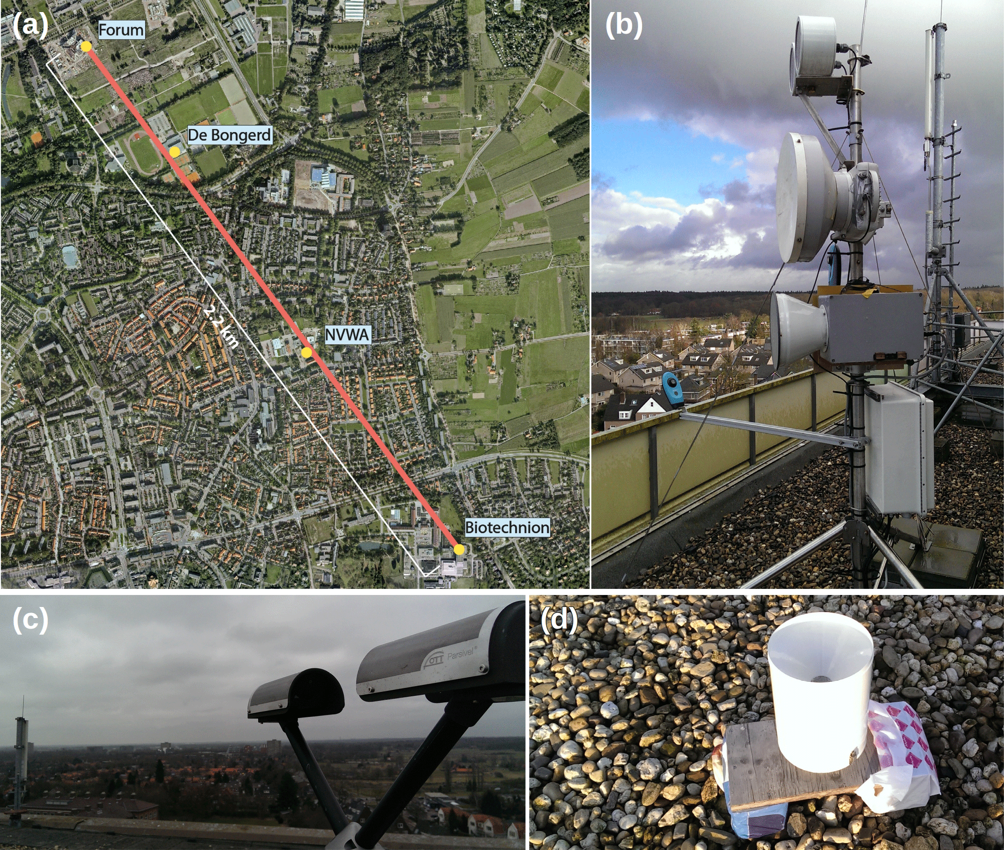
Figure 1 (a) A map of Wageningen showing the path of the links in red. The receiving antennas are at the end labelled “Forum”; the transmitting antennas are positioned at the end labelled “Biotechnion”. The positions of the disdrometers are indicated with yellow dots. Each dotted position houses one disdrometer, except at the “Forum” position, where two disdrometers and an additional tipping bucket rain gauge are placed. (b) The transmitting antenna mast placed on the roof of the “Biotechnion” building. From top to bottom: Scintec BLS900, Nokia Flexihopper (38 GHz) and RAL 26 GHz. The RAL 38 GHz is placed behind the RAL 26 GHz in the photo's perspective and thus not visible. (c) A Parsivel disdrometer (on the “Biotechnion” site). (d) Précis Méchanique tipping bucket rain gauge at the “Forum” site.

The microwave link precipitation detection method is principally intended for liquid precipitation. Snow and hail have different electromagnetic characteristics (i.e. ice has a different refractive index than water, and the shapes of the particles are different). Therefore, different attenuation–precipitation relations hold. Non-melting snow flakes cause very little attenuation in the frequency range under study (e.g. Battan, 1973) and thus we do not expect to be able to detect them. Wet snow hydrometeors, on the other hand, which consists of a mixture of solid and liquid water and air, generally cause more microwave attenuation than a raindrop containing the same amount of water. As we are dealing with more complex shapes and multiple phases of water and air and thus an inhomogeneous index of refraction, accurate estimates of wet snow attenuation and inversely, the estimation of snowfall magnitude through microwave attenuation, poses a real challenge (e.g. Paulson et al., 2011). Nevertheless, we could still detect the presence of wet snow and melting ice pellets.

3 Experimental setup

3.1 Global overview

The backbone of the experimental setup consists of three microwave links placed along the same path between two university buildings on opposite sides of the college town of Wageningen. As such, the majority of the 2.2 km long link path covers urban terrain (Fig. 1a). All transmitting antennas are placed on a 2 m high mast, approximately 1.5 m from the base of the mast (Fig. 1b). The mast is placed on top of a seven storey building. The building is situated atop a slightly elevated area on the south end of Wageningen (51.968657^∘ N, 5.68273^∘ E). The receiving antennas are placed on an identical mast on the roof of an eight storey building at the northern end of Wageningen (51.985230^∘ N, 5.664312^∘ E). The height above ground level is 27 m on the transmitting end and 40 m on the receiving end. The total height above sea level is 62 m at the transmitting end and 51 m at the receiving end. The terrain in between the endpoints of the path consists mostly of terraced housing, a sports field and other buildings of three stories or less. The maximum width of the first Fresnel zone (halfway along the path) at the featured frequencies is less than 5 m. Thus, considering the height of the antenna locations compared to the intermediate terrain, there are no permanent obstructions affecting the beam significantly.

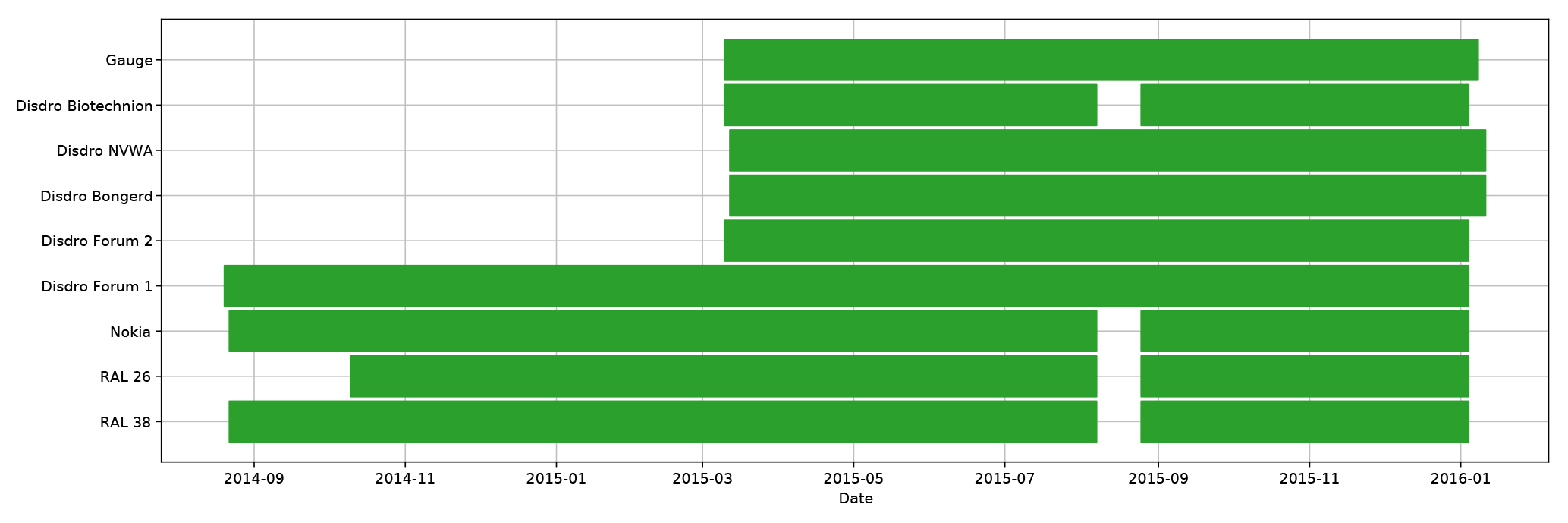
The experiment was operational from 22 August 2014 up to and including 8 January 2016. Not all instruments had been operational during this entire period though, as is indicated in Fig. 2. Also, from 7 to 25 August 2015 all transmitters were nonoperational due to a local power outage.

Figure 2 Operational period per instrument in the experimental setup.

3.2 Microwave and near-infrared links

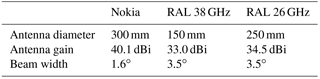
Of the three links one is a Nokia Flexihopper (Nokia), formerly part of a commercial mobile phone network operated by T-Mobile Netherlands. Such links are still used in mobile phone networks around the world and this microwave link could thus be regarded as a typical example of the link systems that would be used in an operational setting. The Nokia is a bidirectional link, but only one receiver was logged in this experiment. It is set to transmit and receive at a frequency of 38.17625 GHz in one direction (which was recorded) and 39.43625 GHz in the other direction. The bandwidth of the signals is 0.9 MHz. The device transmits and receives only horizontally polarized radiation.

The other two links are custom-built by Rutherford Appleton Laboratories (UK) (RAL). The first operates at 26.00000 GHz and transmits and receives only horizontally polarized radiation. It contains both a linear and a logarithmic detector. The second RAL link operates at 38.00000 GHz. The bandwidth of the receivers is 4 KHz, while the transmitted signal bandwidth is extremely narrow (≪1 KHz). Their oscillators are locked to GPS and thus extremely stable. The receiver contains four detectors, two of which measure horizontally polarized radiation (linear and logarithmic) and the other measures vertically polarized radiation (idem). The phase difference between the horizontally and vertically polarized signals is measured by separate detectors as well. In this paper we will only deal with data from the logarithmic detectors. Note that the second RAL link measured at roughly the same frequency as the Nokia link. The frequencies are chosen to be far enough apart so as not to cause interference, but are close enough that the scattering characteristics of the radiation with respect to raindrops are almost identical. Additional characteristics of the link antennas are given in Table 1.

A Scintec BLS900 near-infrared boundary layer scintillometer is also placed together with the microwave links on the same path. It operates at a frequency of 340 THz (880 nm). This provides information about, for example, fog and other visibility-affecting phenomena. Similarly to the microwave links (despite operating in a different scattering regime), it could potentially also be used to estimate rain intensity (Uijlenhoet et al., 2011).

All link receivers are sampled with a Campbell Scientific CR1000 data logger and stored on a remote server on a daily basis. The sampling frequency is 20 Hz. Auxiliary data (e.g. operating temperature) is sampled at a frequency of 2 min⁻¹. The Nokia system consists of separate outdoor and indoor units, the latter containing the digital signal processing circuits and power supply. Note that we have not actively used the indoor unit of the Nokia link system aside from the power supply; Instead, the analogue detector signal normally used for automatic gain control (AGC) is fed directly into the analogue–digital converter (ADC) of the separate data logger. We do this to avoid the significant power quantization error (1 dB) that would be incurred using the link device's own AGC-ADC system. The analogue signal was calibrated in an indoor environment using the signal power indication of the indoor unit as a reference. The RAL links were recalibrated by Rutherford Appleton Laboratories shortly before the beginning of the experiment. The calibration curves are shown below in Fig. 3, and used to convert the observed voltages to received powers. The transmitted power for all devices was kept constant, but was not separately measured.

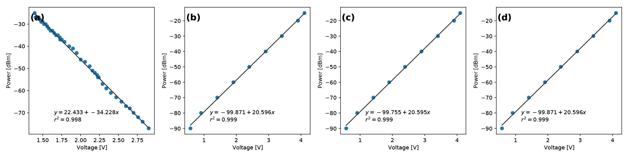
Figure 3 Received signal power vs. detector voltage read-out used for the calibration of the detectors. The black line indicates the fitted calibration curve: (a) Nokia, (b) RAL 38 GHz horizontal, (c) RAL 38 GHz vertical, and (d) RAL 26 GHz.

3.3 Additional instruments

To serve as a ground truth, we use OTT Parsivel laser disdrometers (Fig. 1c). These can not only measure precipitation intensity but also the size and velocity distributions of passing precipitation particles over 30 s intervals. With this information they can provide an approximation of the type of precipitation that occurred. In this manner it is possible to, for example, filter out solid precipitation from the microwave link data or select dry periods to determine the “dry” baseline signal. Due to the small sampling footprint of these devices, they may not give a representative ground truth for the aggregated path measurements. Therefore, five disdrometers are placed at four different locations, spread along the link path (Fig. 1a) as evenly as was possible given the urban terrain. At the receiver end of the link path two disdrometers are placed next to each other in close proximity and orthogonal to each other in order to test the accuracy of the disdrometers themselves. All disdrometers are placed on flat or gently sloping rooftops within Wageningen. The disdrometers all contain a built-in preprocessing unit which samples the raw laser amplitude signals, converts them to hydrometeor counts using an algorithm (undisclosed by OTT) based on the principle described in Löffler-Mang and Joss (2000) and aggregates the samples to 30 s intervals. One of the disdrometers at the receiver end had been operational since the beginning of the experiment. It is connected to the same data logger as the link detectors. The other four disdrometers have been operational for a shorter timespan (see Fig. 2). They are each connected to a UMTS modem, which relays the disdrometer data to a remote server in real time; see Jaffrain et al. (2011) for more details about these autonomous disdrometer stations.

At the receiver end of the link path an automated tipping bucket rain gauge is placed close to the two disdrometers (Fig. 1d), to provide an additional independent measurement. The gauge has a tipping volume of 0.1 mm. Two time-lapse cameras are placed at each end of the link path. On each side one camera is pointed along the path and the other is pointed at the antennas themselves. These serve to allow visual inspection of the link path and the antennas, which can be useful for relating link behaviour to physical events.

For the subsequent data processing we also make use of data from the nearby automatic weather station “Veenkampen” situated roughly 2 km to the west of Wageningen (operated by the university's Meteorology and Air Quality group) for ambient temperature, relative humidity, wind speed, visibility and pressure measurements.

Table 1 Properties of the link antennas used in this experiment.

4 Data processing

4.1 Disdrometers

4.1.1 Preprocessing

The raindrop size and velocity distributions are corrected for known instrumental biases using the method of Raupach and Berne (2015), which involves two steps. Step one is shifting the velocity distributions so that the average velocities per size class match the theoretical terminal velocities for raindrops of that size class. Step two is multiplying the number of detected particles per size class by a class- and rain intensity-dependent correction factor. These correction factors were obtained by Raupach et al. (2015) from concurrent measurements with a 2-D video disdrometer (2DVD), assuming the 2DVD measurements to be unbiased. Using these corrected distributions we derive rain intensities and other bulk quantities.

Whereas Raupach et al. (2015) use the theoretical raindrop terminal velocity model of Beard (1977) to determine the bias in velocity distribution we use the model of Beard (1976). The former is a simplification and approximation of the latter, designed to reduce computational expense. However, we found that on a contemporary desktop computer the time needed to compute terminal velocities was negligible using either model. Both models need the ambient pressure and temperature to calculate the raindrop terminal velocity. We used the temperature and pressure measured by the automatic weather station “Veenkampen”. As this station is situated outside the built-up area of Wageningen, there might be a slight bias in temperature as compared to the urban areas that the disdrometers are situated in.

The model of Beard (1976) does not compute the terminal velocity directly from only the pressure and temperature but instead needs the density of the water drops and ambient air as well as the surface tension of the air–water interface as input. For the density of water as a function of temperature we use the empirical formula of Kell (Battan, 1973). For the surface tension of the air–water interface we employ the empirical relation proposed by Vargaftik et al. (1983).

4.1.2 Derived data

In the subsequent analysis we compare the attenuation encountered by the microwave link signals with the rainfall along the link path. We also make use of a R–k relationship based on the actual rainfall along the path and the expected attenuation due to this rainfall. In order to do so, we assume that the corrected drop size distributions obtained from the disdrometer stations represent the ground truth for that location. The specific attenuation is derived from the drop size distributions using Eq. (3) and Eq. (4). We derive values for a carrier frequency of both 38 and 26 GHz and for both horizontally and vertically polarized radiation.

We calculate the scattering amplitude matrix for each diameter class using the T-matrix approach developed by Waterman (1965). The computations are done using an algorithm adapted from FORTRAN code developed by Mishchenko et al. (1996), Mishchenko and Travis (1998), and Mishchenko (2000) and reimplemented using the Python programming language. As the laser disdrometer cannot provide information on the geometric shape or orientation of the particles, we make use of an orientation averaging scheme. For this purpose we have adapted the particle orientation averaging functions developed by Leinonen (2014) from their T-matrix package. The shape of the raindrops is approximated by an oblate spheroid, with axis ratio dependent on the volume-equivalent diameter. We use the axis ratios suggested by Thurai et al. (2007). The complex index of refraction is needed to calculate the T-matrix. For rain drops we assume the empirically determined formula for the temperature-dependent complex index of refraction for pure liquid water by Liebe et al. (1991) where we use a temperature of 15 ^∘C. Rainfall intensity is calculated with Eq. (2), using the corrected drop size distributions.

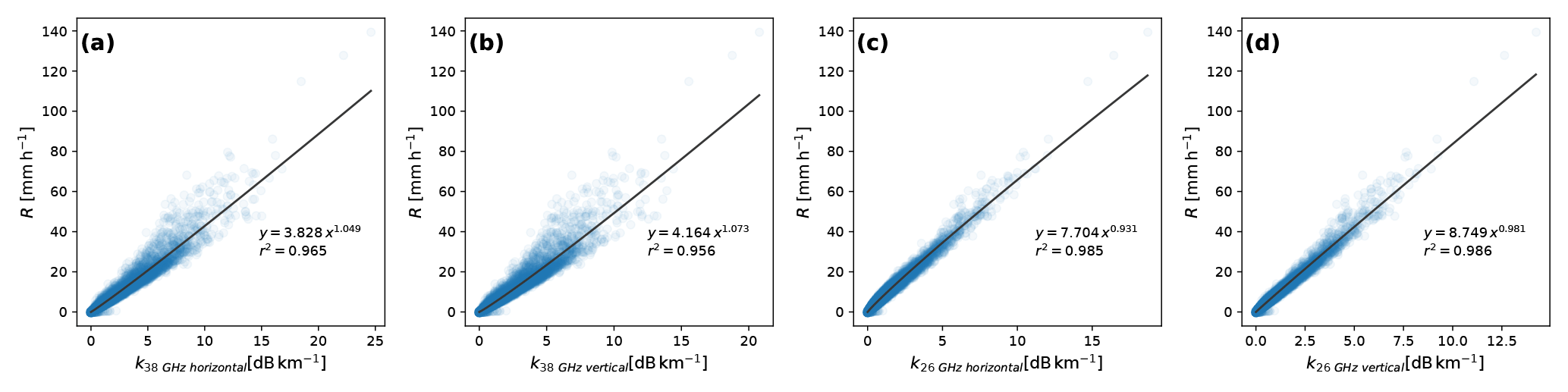
Figure 4 Disdrometer-derived rainfall intensities plotted against disdrometer-derived specific attenuation at several frequencies and polarizations of the incident radiation. The black line indicates the fitted curves: (a) 38 GHz horizontal, (b) 38 GHz vertical, (c) 26 GHz horizontal, and (d) 26 GHz vertical.

In order to provide a comparison for the link measurements, the derived attenuation and rain intensity are then averaged over the link path using a weighted mean over all five disdrometers. For each point along the path, the value of the quantity is taken to be equal to the value derived at the nearest disdrometer. The mean over the path is thus equal to the mean of the disdrometers weighted by the fraction of the path that is closest to that disdrometer. The precipitation type and presence as determined by the Parsivel algorithm are also used. In this case, the path-averaged type is assigned as “mixed” whenever two or more Parsivels register different precipitation types. It is considered “dry” only when all Parsivels agree that there is no precipitation. In all other cases when one or more Parsivels detect precipitation, that precipitation type is assigned as the path-averaged value. We distinguish five broad categories of precipitation: liquid, snow, hail and ice pellets, graupel, and mixed hydrometeors or melting snow. In the subsequent analyses we will mostly be concerned with liquid precipitation, as the other types were rare during the observation period.

Table 2 Coefficients and exponents (a and b parameters) of the R–k relationship derived from different sources for frequencies of 38 and 26 GHz for both horizontally and vertically polarized radiation. Unit of a is mm h⁻¹ dB^−b km^b.

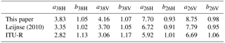
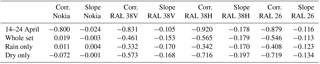
Table 3 Results of the regression of Fig. 11 applied to different subsets of the data.

4.1.3 Rainfall intensity – specific attenuation relationship

The disdrometer-derived rainfall intensities and specific attenuations at the frequencies employed in the microwave links are plotted with respect to each other in Fig. 4. Each dot represents a single 30 s DSD measurement (not path-averaged) from an individual disdrometer. Measurements from all five disdrometers were used. Only data points that were characterized as liquid precipitation by the Parsivel algorithm and where rainfall intensity was higher than 0.1 mm h⁻¹ were selected. These data were then used to fit R–k power-law models using a non-linear least-squares algorithm. Goodness-of-fit for these relationships is very high: R²=0.956 to R²=0.986. Also note that the power-law exponents are all close to one, indicating that specific attenuation and rainfall intensity are nearly proportional to each other at the employed frequencies. These relationships are then applied to the specific attenuations measured with the links.

In Table 2, the determined values are compared with others found in the literature. The values found by Leijnse et al. (2010) were based on drop size distributions collected in the Netherlands as well, but were collected using filter-paper in 1968 (Wessels, 1972). We also compare with the formal ITU (International Telecommunications Union) recommendation regarding the modelling of microwave attenuation due to rain (ITU-R Recommendation, 2005). We see that the exponents (b) are very similar for the relationships obtained in this work and those obtained by Leijnse et al. (2010) and the coefficients (a) found by Leijnse et al. (2010) are 11 to 13 % lower than those found here. We can also conclude that the a parameter is too low (23 to 26 %) and the b parameter is too high (8 to 9 %) in the ITU recommendation with respect to our study for the Dutch rainfall climatology. For the analyses in Sect. 5 we have used these locally derived power laws where applicable.

4.2 Microwave links

In order to calculate the rainfall intensities, the attenuation caused by rainfall and the attenuation caused by other atmospheric effects must be distinguished. Rahimi et al. (2003) proposed a two-step approach in order to do so.

The first step is to determine which of the sampled periods are dry. Overeem et al. (2013) uses the assumption of spatial correlation of rainfall to determine “wet” and “dry” periods for microwave links in cellular communication networks. In short, a period is considered “wet” if nearby links show a mutual decrease in received signal levels. As we are considering only a single path, such a method would not be applicable here. An alternative is to use the assumption of temporal correlation of rainfall. Schleiss and Berne (2010) suggest using a moving window standard deviation threshold. Similarly, Chwala et al. (2012) used a Fourier-transform based method to distinguish between wet and dry spells. Other methods applicable to a single link path are e.g. a Markov switching algorithm (Wang et al., 2012) and the use of dual-frequency links (Rahimi et al., 2003). Here, the path-aggregated disdrometer data is used to determine dry periods independently of the microwave link data.

The second step in the algorithm is to determine a suitable baseline signal level using the selected dry periods. The implemented baseline algorithm uses a rolling median over all measurements classified as dry in the surrounding centred 24 h period to determine the baseline signal for each time step. The specific attenuation is then calculated as

$$\begin{array}{}\text{(7)}& k=\max \left({\displaystyle \frac{R{x}_{\mathrm{ref}}-Rx}{L}},\mathrm{0}\right),\end{array}$$

where Rx is the received power and L is the path length. Rainfall intensity is derived from the corrected attenuation using the power-law relationship of Eq. (5). The parameters a and b in this equation are obtained from the disdrometer data as described in Sect. 4.1.3.

Futhermore, the rainfall intensity is set to 0 when the disdrometer indicates dry weather. Note that we do not perform any a priori additional corrections on the microwave link rainfall estimate, such as correcting for wet antenna attenuations. The goal is, after all, to use this basic estimate to assess potential error inducing phenomena, not to evaluate a best-effort estimation.

5 Results and discussion

5.1 Overview

In the following section, we use the rainfall intensity as measured by the Parsivel disdrometers as a reference to assess the link-derived rainfall. Unless stated otherwise, we use the corrected DSD-derived rainfall intensities, not the rain intensities that the internal Parsivel algorithm produces.

In order to better understand the different phenomena that contribute to the microwave link attenuation signal, we present a number of illustrative events from the dataset. We search for events that can be related to a single type of attenuating phenomenon in order to gain insight into the separate phenomena. We will first analyse the performance of the simple algorithm for measuring liquid precipitation and take a quick look at solid and mixed precipitation. We will then show how temperature and wet antennas, e.g. caused by dew formation affect the signal. Finally, we will look at some currently unexplained phenomena and also give some examples where different phenomena occur simultaneously. All times in the description of the events are given in UTC.

5.2 Rainfall events

We compare the link-derived rainfall rates using the simple algorithm (excluding any specific corrections) described in Sect. 4.2 with the spatially averaged rainfall rates derived from the disdrometers using the corrected DSDs. To assess the reliability of the disdrometer measurements as a ground truth, we first compare the collocated disdrometers with the tipping bucket rain gauge and each other. We used data of the entire measurement period where rain intensities higher than 0.1 mm h⁻¹ were registered. We find that the correlations of the disdrometers with the rain gauge (r=0.928 and r=0.927) were only slightly lower than the correlation of the disdrometers with each other (r=0.959). The mean differences between the disdrometers and the rain gauge were 0.039 and 0.129 mm h⁻¹, respectively, while the mean difference between both disdrometers amounted to 0.074 mm h⁻¹. That means that the disdrometers slightly overestimate the rain intensities as compared to the rain gauge, but this is of the same order of magnitude as the differences between the identical collocated disdrometers. Therefore, we will assume the path-averaged disdrometer measurements to be the “true” path-averaged rainfall for the purpose of evaluating the link measurements.

Figure 5 shows an example of a single short isolated rain event on 14 July 2015 as indicated by the disdrometers. We chose this example because there are no attenuating phenomena contributing to the dynamics of the signal other than rain in this event. Note that the received signal level of the Nokia is offset by 14 dB in order to fit into the plot. This is done consistently for all following figures. As the received power level can vary within the dry periods that we use to determine the baseline power level, we also indicate the 95th and 5th percentile of the received power level over the dry intervals within the surrounding 24 h moving window. This gives an indication of the variability of the baseline power level. Thus, if the rain-induced attenuation is within this range, it cannot be distinguished from variability in the baseline without further processing. The event consists of two distinct small peaks. The first peak of the path-average rainfall intensity only reaches 0.7 mm h⁻¹, while the second peak reaches 8 mm h⁻¹. We see that the second peak causes a clear attenuation of the received signal level of all the links. The smaller peak in rain intensity causes only a small attenuation in the 38 GHz links, fully within the 95th and 5th percentile range of the dry signal. Although the presence of rainfall is detected unambiguously by all the instruments, the magnitude of the response differs between the links. Both the horizontally and vertically polarized detectors in the 38 GHz RAL link give very similar responses, which is expected as they receive different components of the same signal and also share a substantial part of their electric signal path, including the antenna itself. Most notable is the difference between the signal of the Nokia link and the RAL link operating at (nearly) the same frequency and polarization. Although the magnitudes are similar, the Nokia link has far less variability of the baseline signal level than all other link instruments. This difference could be caused by the differences in internal electronics of the detector. Another point of interest is that using the median of all dry data points in the 24 h period, our estimation of the baseline signal level of the 26 GHz RAL link and to a lesser extend the 38 GHz RAL link is too high, resulting in an additive overestimation of the rain intensity. The calculated apparent rainfall during the first peak is completely below this line, indicating that this can be regarded as noise. Regardless, the peak rainfall estimate from the Nokia link is very close to the disdrometer estimate. We can also see that attenuation of the microwave link signal persists for several minutes after the end of the rainfall event (according to the disdrometers) and slowly decays during this time. This could be the consequence of the link antennas becoming wet due to the rain and subsequently drying up after the event (Minda and Nakamura, 2005; Leijnse et al., 2008). In Fig. 5a the received signal level of the near-infrared link is also plotted. Attenuation of this signal is indicative of visibility. In this case the visibility loss is highly correlated with rain (correlation coefficient $r=-\mathrm{0.86}$).

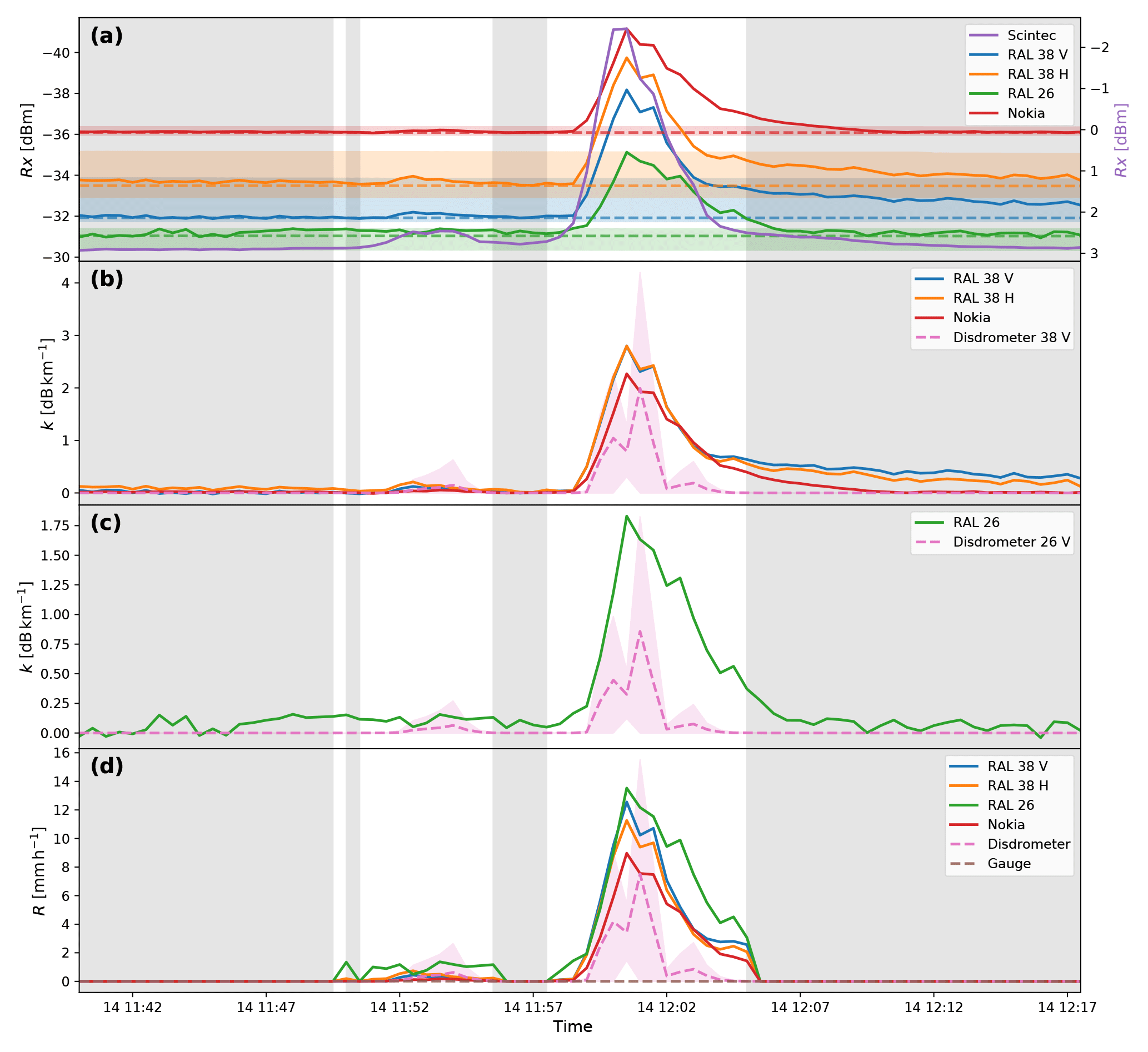
Figure 5 Time series of an event on 14 July 2015. (a) Received power levels (solid lines) and reference levels (median over dry periods in a 24 h moving window: dashed lines). The 5th and 95th percentile power level over dry periods in a 24 h moving window are indicated by the coloured shading. (b) Specific attenuation of the 38 GHz links derived using the reference levels as well as the theoretical specific attenuation at 38 GHz derived from the disdrometers. Both the weighted spatial average (dashed line) and weighted spatial standard deviation (shaded area) are shown. Panel (c) is the same as (b), but for 26 GHz. (d) Rainfall intensities derived from the link attenuations using the R–k power law and rainfall intensities derived from the disdrometers. Both the weighted spatial average (dashed line) and weighted spatial standard deviation (shaded area) are indicated. The rainfall intensities derived from the tipping bucket gauge are indicated with the brown dashed line. Dry periods, as determined with the disdrometers, are represented by grey shaded areas.

We illustrate the response of the link signals to rain with two more example events of a longer duration. One low-intensity drizzle event and one higher-intensity convective rain event with some spatial heterogeneity. On both occasions we use only the times for which at least one of the disdrometers indicate rain has occurred for further analyses.

The first event, on 24 November 2015, consists of a low-intensity drizzle period (intensities under 2 mm h⁻¹ for most of the event) that persists for around 12 h. The course of the event is illustrated in Fig. 6. The RAL links show some variability in the baseline power level, varying over a range of 0.11 to 0.14 dB over the course of the event until 13:00 UTC. The Nokia link, in contrast, stays remarkably stable during the entire event, ranging only 0.02 dB over the same period. After that, all links show a large drop in baseline power level, with the largest magnitude in the RAL 38 GHz link (3.46 dB) and the smallest in the Nokia link (0.33 dB). There is a fairly strong correlation of link derived rain intensity with disdrometer rain intensity for both the Nokia link and the 26 GHz RAL link (r=0.870 and r=0.854, respectively) and less so for the 38 GHz RAL link (r=0.594 for vertical polarization and r=0.232 for horizontal polarization).

We estimate the additive and multiplicative bias in the link-derived rain intensity by the parameters of a simple linear regression with the spatial average of the disdrometer derived rainfall, which is illustrated in Fig. 7a–d. All microwave links overestimate the rain intensity to some extent. Additive bias of the RAL links is between 2.2 and 3.7 mm, which is more than the actual rainfall during most of the event. Additive bias is lowest in the Nokia link-derived data, which seems to be in line with the very stable baseline. However, it is still 0.8 mm h⁻¹, which is a problem for accurately measuring accumulations from light rain events. We can also see that in this case visibility cannot be reliably used as a proxy for rainfall intensity, as is most clearly seen after 13:00.

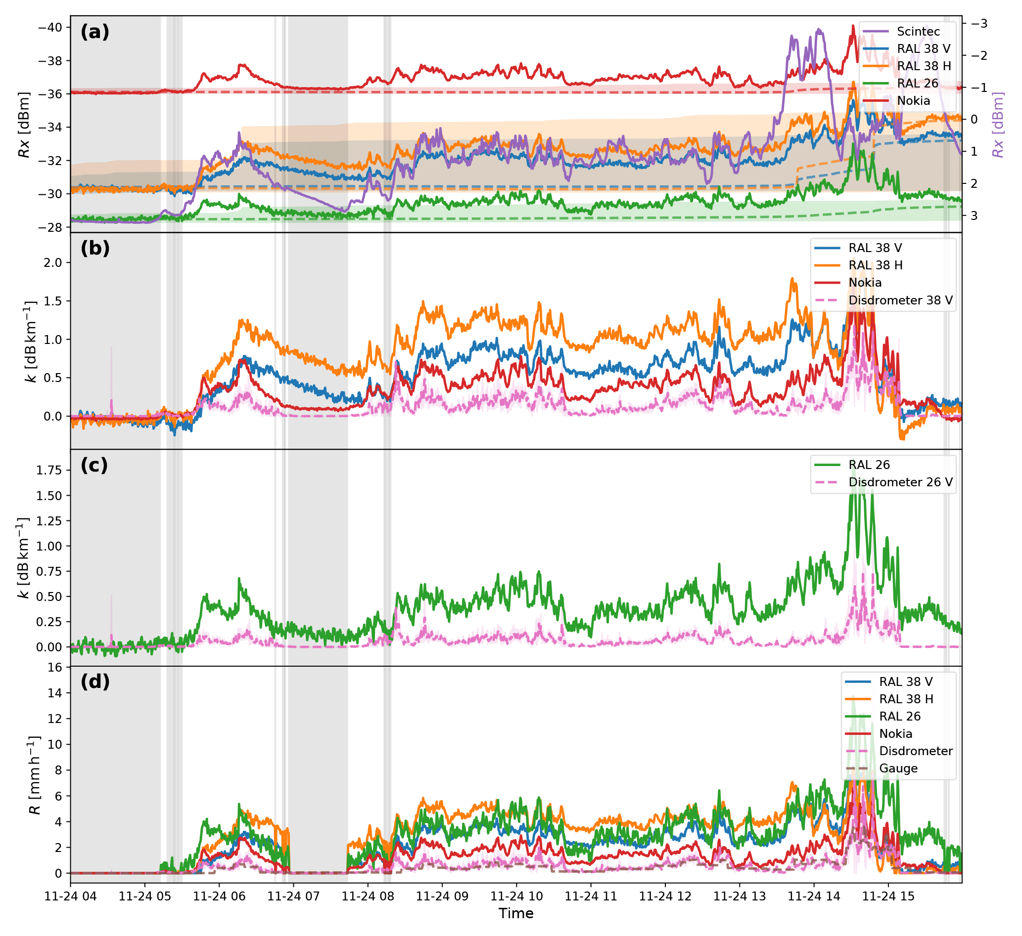
Figure 6 Time series of an event on 24 November 2015. (a) Received power levels (solid lines) and reference levels (median over dry periods in a 24 h moving window: dashed lines). The 5th and 95th percentile power levels over dry periods in a 24 h moving window are indicated by the coloured shading. (b) Specific attenuation of the 38 GHz links derived using the reference levels as well as the theoretical specific attenuation at 38 GHz derived from the disdrometers. Both the weighted spatial average (dashed line) and weighted spatial standard deviation (shaded area) are shown. Panel (c) is the same as (b), but for 26 GHz. (d) Rainfall intensities derived from the link attenuations using the R–k power law and rainfall intensities derived from the disdrometers. Both the weighted spatial average (dashed line) and weighted spatial standard deviation (shaded area) are shown. The rainfall intensities derived from the tipping bucket gauge are indicated with the brown dashed line. Dry periods, as determined with the disdrometers, are represented by grey shaded areas.

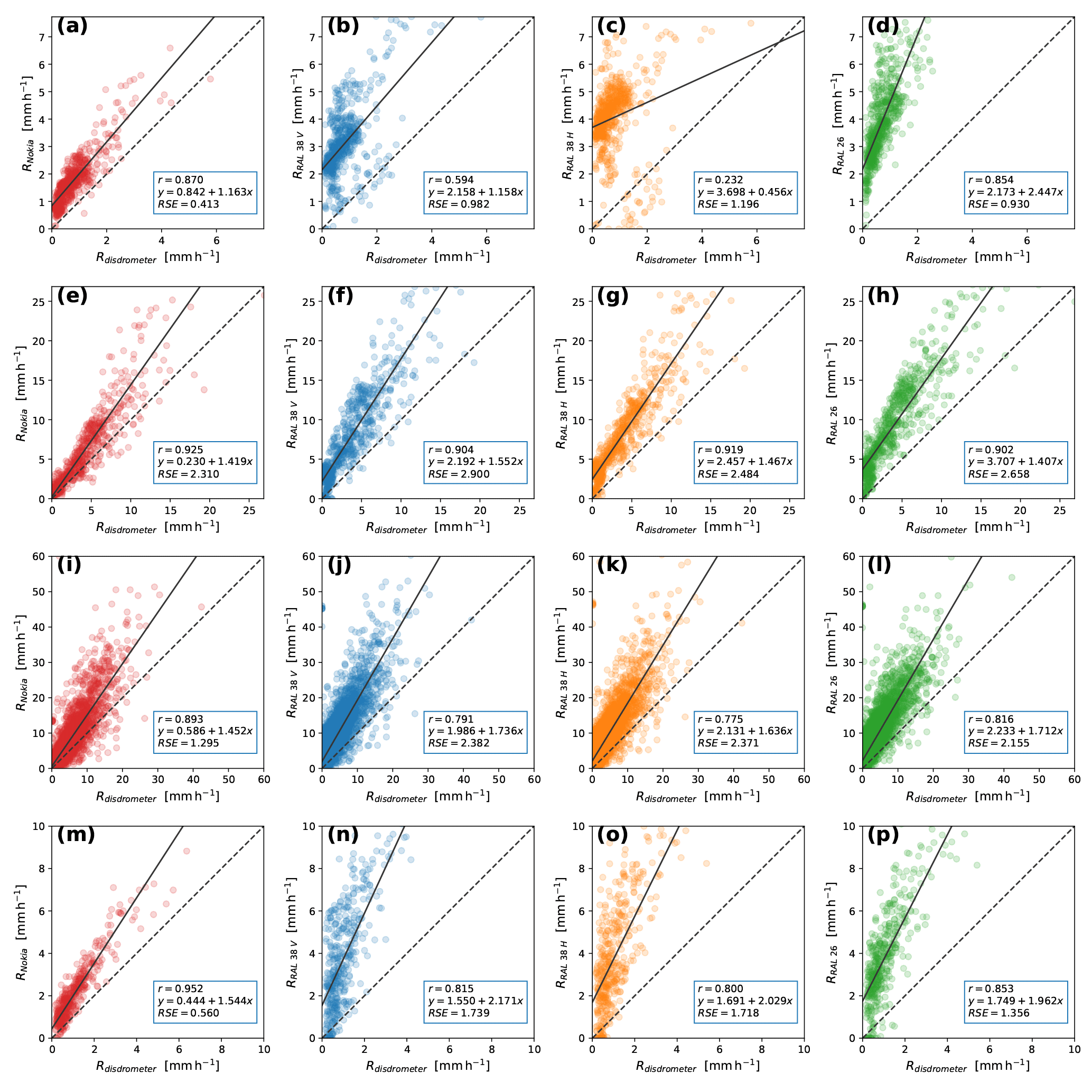
Figure 7 Scatterplots of link-derived rainfall intensities vs. disdrometer-derived rainfall intensities. Solid lines indicate a linear least-squares fit, dotted lines indicate the 1:1 line. Within each plot the correlation coefficient (r), the fitted line function and the residual standard error (RSE) are also shown. Links from left to right: Nokia, RAL 38 GHz vertical, RAL 38 GHz horizontal, and RAL 26 GHz. From top to bottom: 24 November 2015 (down-sampled to 30 s), 4 November 2015 (down-sampled to 30 s), whole dataset down-sampled to 30 s, and whole dataset down-sampled to 15 min.

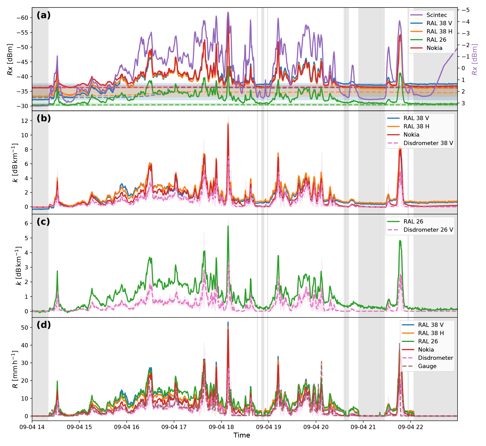
Figure 8 Time series of an event on 4 November 2015. (a) Received power levels (solid lines) and reference levels (median over dry periods in a 24 h moving window: dashed lines). The 5th and 95th percentile power level over dry periods in a 24 h moving window are indicated by the coloured shading. (b) Specific attenuation of the 38 GHz links derived using the reference levels as well as the theoretical specific attenuation at 38 GHz derived from the disdrometers. Both the weighted spatial average (dashed line) and weighted spatial standard deviation (shaded area) are shown. Panel (c) is the same as (b), but for 26 GHz. (d) Rainfall intensities derived from the link attenuations using the R–k power law and rainfall intensities derived from the disdrometers. Both the weighted spatial average (dashed line) and weighted spatial standard deviation (shaded area) are shown. The rainfall intensities derived from the tipping bucket gauge are indicated with the brown dashed line. Dry periods, as determined with the disdrometers, are represented by grey shaded areas.

The second event, on 4 November 2015, is more spatially heterogeneous (CV = 0.64, as opposed to CV = 0.50 in the previous event.). The higher spatial heterogeneity and higher rainfall intensities suggest a convective rainfall event. The total event lasts for 8 h (see Fig. 8). Peaks in spatially averaged rainfall intensity during this event are on the order of 20 to 30 mm h⁻¹, and individual disdrometer measurements reach up to 55 mm h⁻¹. Once again the baseline of the Nokia link is remarkably stable (range = 0.19 dB), similar to the 26 GHz RAL link (range = 0.33 dB), while the 38 GHz RAL link has a highly variable baseline (range = 1.53 dB for the horizontally polarized signal and 3.96 dB for the vertically polarized signal). During most of this event visibility seems to be a reasonable proxy for the rainfall intensity. Correlations of link-derived rainfall with disdrometer-derived rainfall are much higher overall (r=0.90 to r=0.93) (Fig. 7e–h) than for the event on 24 November 2015. Additive bias is of the same order of magnitude as for the drizzle case, which means that the additive bias relative to the rainfall intensities is much less for this event than for the drizzle event. Multiplicative bias varies from a factor of 1.4 to 1.6.

We now compare link derived rain intensity with disdrometers derived rain intensity for the entire measurement period; results are shown in Fig. 7i–l. Data points where the path-average rainfall intensity derived from the disdrometer measurements are less than 0.1 mm h⁻¹ or at least one of the disdrometers indicate the presence of solid precipitation are excluded. We also exclude the period during which the link transmitters were not functioning. The Nokia link performs better than the RAL links in terms of correlations. In all cases the links significantly overestimate the rainfall intensity, both in an additive (regression intercept ranging from 0.6 to 2.2 mm h⁻¹) and a multiplicative (regression slope ranging from 1.5 to 1.7) sense. The general overestimation could be attributed to attenuating phenomena other than rain being erroneously processed as rain in the basic algorithm, in part due to the simple baseline determination process not taking these into account and because e.g. no correction was applied for wet antennas. A similar regression in terms of specific attenuations produces nearly identical results. Therefore, we conclude that uncertainties in the R–k relation do not significantly explain uncertainties in the rainfall estimation.

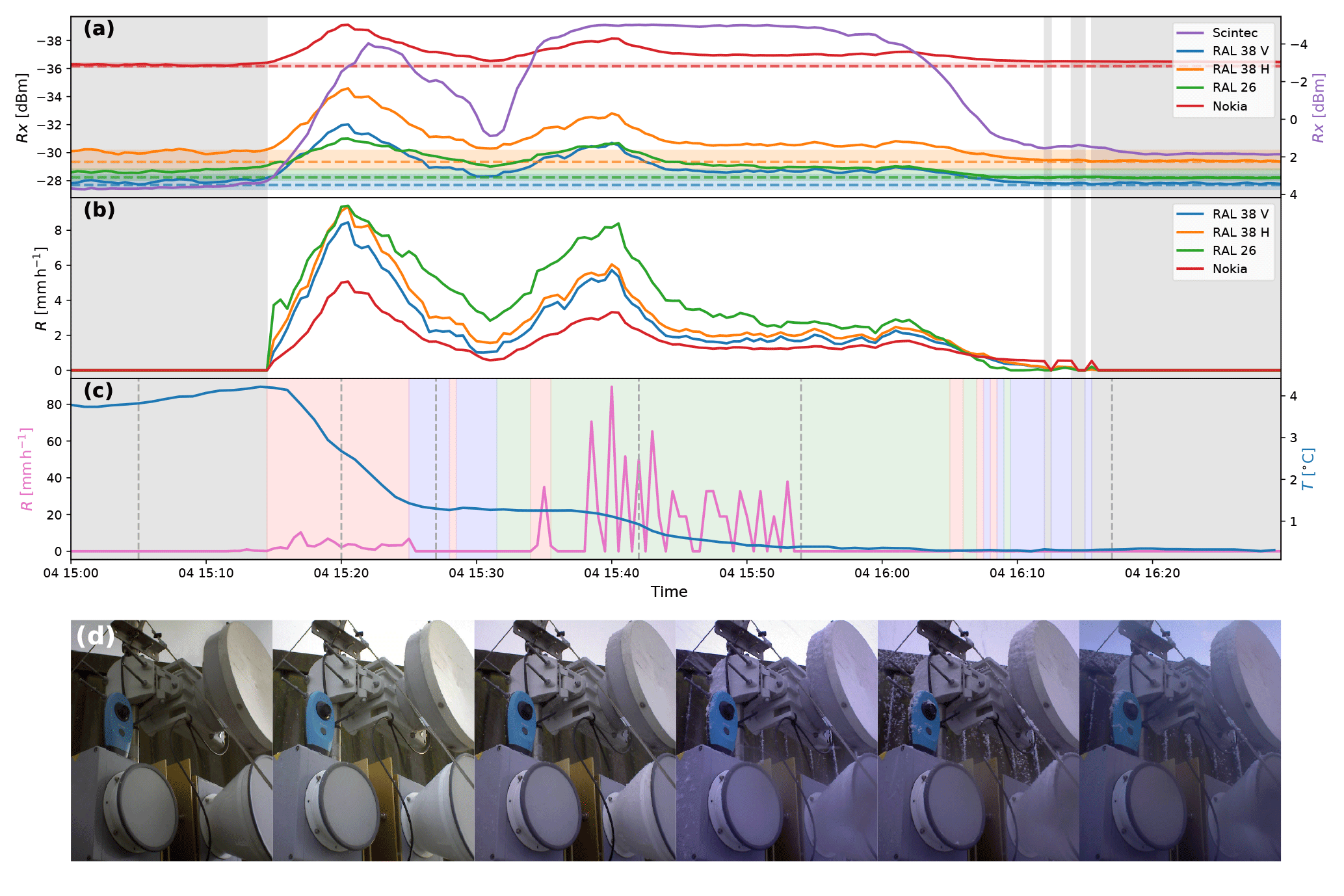
Figure 9 Time series of an event on 4 February 2015. (a) Received power levels at the detectors (solid lines) and reference levels (median over dry periods in a 24 h moving window: dashed lines). The 5th and 95th percentile power levels over dry periods in a 24 h moving window are indicated by the coloured shading. (b) Derived rainfall intensities using the basic algorithm. (c) Rainfall intensities derived from the disdrometer positioned at “Forum” and ambient air temperature at 2 m at the “Veenkampen” meteorological station. Dry periods, as determined with the disdrometers, are represented by grey shaded areas. Periods with mixed precipitation are indicated with red shaded areas; periods where only liquid precipitation is detected are indicated in blue; and periods with snow are indicated in green. (d) Images from the time-lapse camera at the location of the transmitting antennas aimed at the antennas. The times at which these images were capture are indicated by the vertical dashed lines in (c).

In typical operational settings, longer temporal measurement intervals such as 15 min are common (e.g. Overeem et al., 2016b). In order to illustrate the performance of a basic algorithm without any sort of correction at this resolution, Fig. 7m–p show the scatterplot and linear regression for the entire dataset, but down-sampled using a 15 min mean. The correlation for the Nokia link is slightly higher with the 15 min intervals than it is using 30 s intervals and the scatter around the regression line is lower. In the case of the RAL links, the performance is better for the 15 min accumulations than for the 30 s intervals in terms of correlation and scatter, but worse when considering bias.

5.3 Solid/mixed precipitation

Very few solid or mixed precipitation events occurred during our measurement period. Figure 9 shows one of the few snowfall occurrences during the campaign, on 4 February 2015. At this point in the campaign only one disdrometer was yet placed and no rain gauge was available, which limits the potential for a quantitative comparison. Figure 9d shows time-lapse camera footage taken during different stages of this event. The background shades in Fig. 9b indicate the type of precipitation as indicated by the Parsivel internal algorithm (blue is liquid precipitation, green is snow, red is mixed precipitation). The total event duration is about 40 min, yet the event is quite variable in time.

As indicated by the background colours and the camera footage, this short event starts out with a mixture of rain and ice pellets and then turns into snowfall. Along with the mixed precipitation the temperature drops from 4 to 1 ^∘C. During the snowfall, the temperature drops further to 0 ^∘C. The absolute values of the disdrometer-derived precipitation intensity cannot be taken at face value here, as our processing algorithm treats every particle as a raindrop. This results in far too high values during snowfall, as we do not account for the lower density of a typical snowflake. As the disdrometer rainfall intensity shown here is that of only one disdrometer and as it was placed at one far end of the link path, we do not expect the small-scale variations to match exactly with those of the link attenuation. However, the overall dynamics of the intensity and the type of precipitation can provide some useful information.

Between 15:10 and 15:30, the links are attenuated with a magnitude that corresponds roughly with the precipitation intensity measured by the disdrometer, assuming that it is pure rain. Afterwards, when snow starts to fall between 15:30 and 15:55, the precipitation intensity derived from the disdrometers becomes a factor of 10 higher than the link-derived precipitation intensity, but this is likely to be due to the faulty disdrometer algorithm when applied in snow. While both the disdrometer and the camera footage seem to indicate that the precipitation stops after 15:55, the attenuation of the links persists until the signal level returns to its initial value between 16:00 and 16:15. At this point the temperature hovers at a few tenths of degrees above zero, and the camera footage indicates some residual snow is left on the antenna covers. The snow deposits are mostly on top of the covers and is mostly still present by 16:17, when attenuation has decayed fully, so snow deposits alone cannot explain the persistent attenuation. Based on the above observations a possible explanation of the persistent attenuation effect would be the partial melting of residual snow on top of the antenna cover, which then keeps the antenna cover wet. However, the available data is not sufficient to confirm this.

Because there were few snowfall events during the entire campaign period and each of them was of short duration and mixed with other types of precipitation (similar to the event described in this section), no meaningful analyses could be done regarding the relationship between attenuation and snowfall intensity.

5.4 Temperature

Throughout the entire observation period a diurnal oscillation can be seen in the attenuation signal. This diurnal cycle is present in all signals, although the magnitude of the oscillation is in general significantly higher for the RAL links (1.0–1.5 dB) than it is for the Nokia link (∼0.2 dB). The magnitude of the oscillation also varies throughout the observation period. This behaviour does not correspond to any precipitation pattern but seems to follow the known diurnal variations in temperature. Although this pattern can be seen throughout the observational period, the correlation with temperature is not always clear, because the signal is generally much weaker when other attenuating phenomena are present.

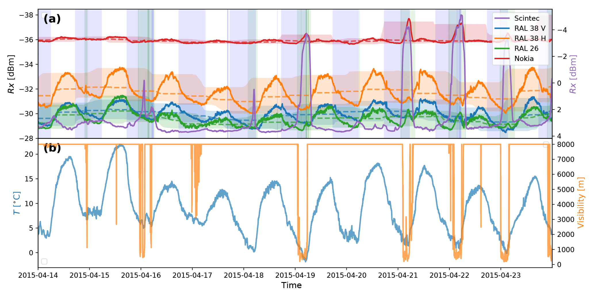
Figure 10 Time series of the period between 14 April 2015 and 24 April 2015. (a) Received power levels (solid lines) and reference levels (median over dry periods in a 24 h moving window: dashed lines). Periods with a negative net radiation flux at the surface are indicated with blue shading. Periods with a relative humidity >90 % are indicated with green shading. (b) Several atmospheric variables measured at the “Veenkampen” meteorological station: visibility and ambient air temperature at 2 m indicated with orange and blue lines, respectively.

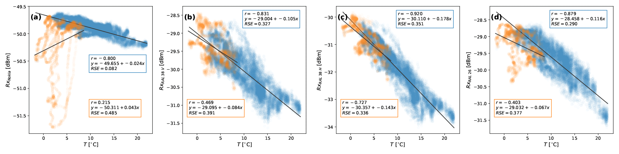
Figure 11 Scatterplots of link received power vs. ambient air temperature measured at the “Veenkampen” meteorological station. Blue dots indicate times when relative humidity (as measured at “Veenkampen”) is <90 %; orange dots indicate times when relative humidity >90 %. Solid lines indicate linear least-squares regression fit. Links: (a) Nokia Flexihopper, (b) RAL 38 GHz vertical, (c) RAL 38 GHz horizontal, and (d) RAL 26 GHz.

Therefore, we will first focus on a relatively long dry period between 14 and 24 April 2015, as shown in Fig. 10. During this period the disdrometers picked up no precipitation; however, the received signal levels are not constant. Instead, variations up to 1 dB are present. In Fig. 10b, the time series of ambient air temperature measured by the nearby weather station is plotted for the same period together with the visibility measured at that same station, while in Fig. 11, the power levels for this period are plotted against the temperature with a simple linear regression. We performed separate regressions for instances where humidity was above 90 % and for instances where relative humidity was below 90 %. This was done to distinguish instances where dew formation on the antennas might have occurred, which we will discuss in the next subsection. In Fig. 10a we have also indicated the periods where relative humidity is above 90 % (green shade) and the periods where the net radiation flux towards the surface is negative (blue shade).

There is a strong negative correlation between received power and temperature for all link instruments (r=0.80 to r=0.92), when relative humidity is below 90 %. However, the slope of the linear fit is much lower for the Nokia link (−0.024 dB K⁻¹) than for the others (between −0.1 and −0.2 dB K⁻¹), even though the Nokia link operates at (nearly) the same frequency and polarization as one of the RAL links. Apparently, the magnitude of the temperature dependence is far more specific to the link hardware, than to the carrier frequency or polarization. The negative correlation between temperature and received power in the RAL devices is much milder when the relative humidity is above 90 % ($r=-\mathrm{0.40}$ to $r=-\mathrm{0.72}$). For the Nokia link, the temperature dependence disappears at high humidity. This phenomenon is probably related to dew formation at the antennas as is discussed in more detail in Sect. 5.5.

In subsequent analyses we expand our investigation of a possible linear temperature dependency to the entire experimental period. However, we exclude two time frames from this analysis. Firstly, the period between 6 and 25 August 2015 when the transmitters were not functioning (but the receivers were). Secondly, we also exclude a period between 11 and 19 May 2015 because a metal construction crane was positioned in the line of sight between the transmitter and receiver (see Sect. 5.7) several times in this period. The correlations and regression slopes found for this extended period are shown in Table 3 as “whole period”.

We consider that dew-related wetting of antennas causes attenuation of the link signal, which muddles the observed temperature dependency. Furthermore, this phenomenon seems only to occur when the nearby weather station registers a relative humidity above 90 %. Therefore, we filter the dataset in two more ways in order to separate temperature effects from signal attenuation in the full time period. First, we remove all data points where any disdrometer indicates any form of precipitation. Second, we remove all data points where relative humidity was above 90 %. We then find the correlations and slopes indicated in Table 3 as “dry only”. Furthermore, for completeness we also show correlations and slopes for a subset where, instead of the two abovementioned filters, we apply a filter that only includes periods where any of the disdrometers registered rain (shown in Table 3 as “rain only”).

The slopes of the linear regression for the RAL links are similar for all data selections (difference within ±15 % compared to the slopes found for 14–24 April), while the correlation coefficients become progressively smaller for the “dry only” selection ($r=-\mathrm{0.57}$ to $r=-\mathrm{0.72}$), the “whole set” selection ($r=-\mathrm{0.46}$ to $r=-\mathrm{0.57}$) and the “rain only” selection ($r=-\mathrm{0.33}$ to $r=-\mathrm{0.41}$). The latter is still surprisingly high considering that the received signal level in this selection includes attenuation by rain. For the Nokia link no significant correlation of received power level to temperature is found for any of the data selections, even though one would expect it based on the findings from 14–24 April.

5.5 Dew and fog

There is also another phenomenon apparent in Fig. 10, especially noticeable in the Nokia link: some sharp drops in received power that evolve from midnight until the early morning (∼ 00:00–05:00) and then quickly disappear again within 2 h with peaks of 1 to 2 dB (see Fig. 10a). Comparing to Fig. 10b, it is clear that they do not coincide with any change in temperature. Instead, these peaks only appear in periods when the net radiation is negative and the relative humidity is above 90 %. The power gradually returns again to the previous level when the net radiation becomes positive and the event is over as soon as the relative humidity drops below 90 %. From Fig. 10 we can see that these instances (where humidity is above 90 %) are not correlated to temperature. These characteristics indicate that dew formation on the antennas is a plausible explanation for this phenomenon. The hypothesis is as follows: relative humidity in the air approaching 100 % and a net loss of radiative energy at the surface are indicative of dew formation; water condenses on the antenna covers and builds up a thin layer of water which causes attenuation proportional to the thickness of the layer (see Leijnse et al., 2008); as the net radiative flux changes sign and the water layer dries up, the attenuation slowly returns to the baseline level.

Fog and dew often occur under the same conditions and it is thus difficult to rule out fog as the principal cause, from correlations alone. If we take the visibility as indicative of the amount of fog, then we can see that they indeed occur often (but not always) at the same time.

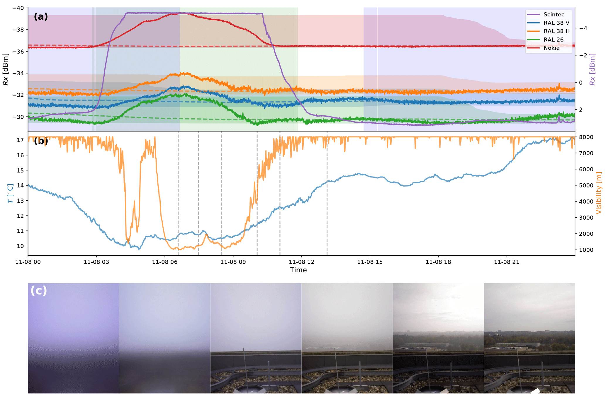
Figure 12 Time series of an event on 8 November 2015. (a) Received power levels at the detectors (solid lines) and reference levels (median over dry periods in a 24 h moving window: dashed lines). Periods with a negative net radiation flux at the surface are indicated with blue shading. Periods with a relative humidity >90 % are indicated with green shading. (b) Several atmospheric variables measured at the “Veenkampen” meteorological station: visibility and ambient air temperature at 2 m indicated with orange and blue lines, respectively. (c) Images from the time-lapse camera at the location of the receiving antennas aimed along the link path. The times at which these images were captured are indicated by the vertical dotted lines.

In the case shown in Fig. 12, a different fog event is shown in more detail. In this case, time-lapse camera footage was available for a significant portion of the event, and is shown in Fig. 12c. Here again, strong attenuation is experienced by all the links with a peak attenuation of 3 dB in the case of the Nokia link, yet none of the disdrometers detect precipitation. Therefore, it is likely that we are dealing with a different attenuating phenomenon than precipitation. Using the basic rainfall retrieval algorithm, this event would result in an accumulated rainfall depth of 26 mm. As the time series of attenuation is smoother than we would expect of rainfall, we are likely dealing with antenna wetting due to either dew formation, or the result of fog. The effect of fog on microwave link attenuation has also been observed by, e.g. Liebe et al. (1989) and David et al. (2013). However, as mentioned in those studies, the theoretical attenuation by fog droplets themselves is only 0.75 dB at 38 GHz for a 1 km path and a very high liquid water content of 0.8 g m⁻³. Therefore, no more than 1.5 dB attenuation can be expected due to the fog itself and an attribution to fog must also include the wetting of the antennas. Observation of the accompanying time-lapse camera footage (Fig. 12c) reveals a heavy fog during the early morning, which gradually clears up concurrently with the decrease in attenuation in the late morning. No camera footage was available at night during the increasing leg of the attenuation signal, because the cameras cannot record during low-light. However, comparison of the visibility data from the nearby weather station (Fig. 12b) with the pattern of attenuation, seems to undermine a direct relationship with fog. Visibility measurements from the NIR link along the path itself are of limited use in this case, as the fog is so heavy that the attenuation is “saturated” for most of the duration. The striking correspondence of the sign switch of both net radiation and attenuation increase makes dew formation the most likely interpretation.

5.6 Wet antennas

Near the start of the measurement period a simple test case was performed to assess the effect of wet antennas on rainfall retrieval. During a dry sunny day (12 September 2014), while the ambient temperature was 21 ^∘C, both the Nokia and the RAL 38 GHz receiving antennas were artificially wetted in short bursts using a spray bottle. The antennas were wetted until visually saturated and then allowed to dry in the sun. In this way, the attenuating effect of wet antennas can be observed, decoupled from the attenuating effect of raindrops in air. The RAL 26 GHz link was not included in the test, as it was not yet installed at the time; however, the antenna cover design and material is identical to that of the RAL 38 GHz link (aside from its diameter) and thus it is assumed that the effect is similar.

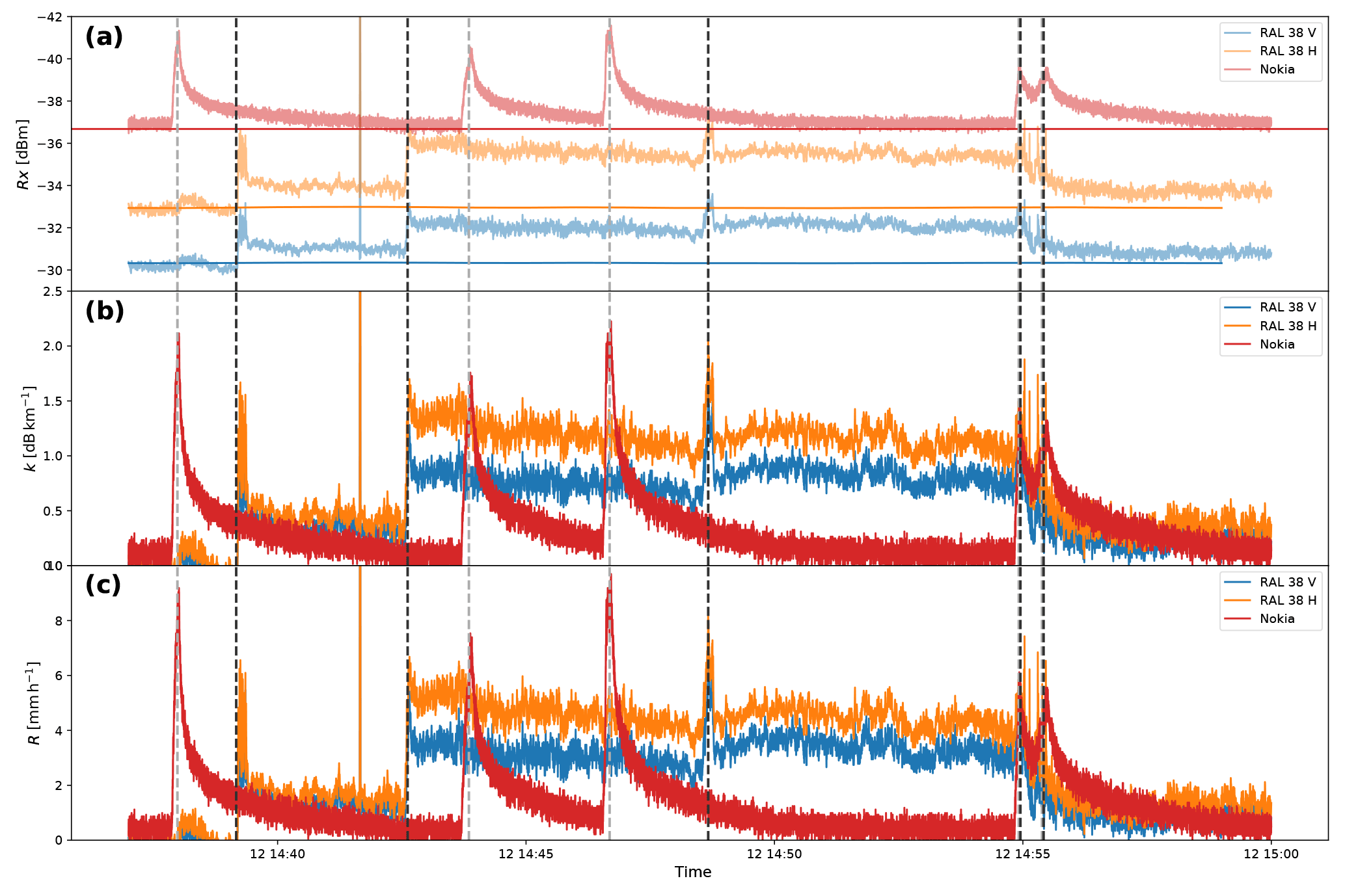
Figure 13 Time series of the wet antenna experiment on 12 September 2014. (a) Received power levels at the detectors, with the reference levels indicated in darker hues. The reference levels are singular values manually fitted for this event. These are the raw 20 Hz sampled data, not the 30 s resampled data. The dotted vertical lines indicate the moments when a water spray was applied, with the dark grey lines indicating sprays on the RAL antenna and the light grey lines indicating sprays on the Nokia antenna. (b) Specific attenuation of the links. (c) Derived rainfall intensities using the R–k power law.

Figure 14 Photographs of the receiving antenna covers, during the wet antenna experiment, taken just after the antennas were sprayed. Panels (a) and (b) are two instances of the RAL 38 GHz cover. Panel (c) is the Nokia Flexihopper cover.

In Fig. 13a the resulting attenuation signal is shown. It is seen that wetting of one antenna of the Nokia link system can result in an extra attenuation of 3 to 5 dB, which is of the same order of magnitude as what is observed in dew and fog events (where presumably both antennas of a link are affected). This corresponds with a rain intensity of 15 to 22 mm h⁻¹ using the power law derived in Sect. 4.1.3 (shown in Fig. 13b). The signal then follows an exponential decay pattern due to drying, where the time for the attenuation to decrease by 95 % is 3 min. The RAL link response to wetting is completely different, which may be related to the way water collects on the antenna cover surface. The extra attenuation due to wetting is only 1 to 3 dB and the decay has two distinct stages. The initial peaks drop in less than a second after the spray stops, with no discernible decay pattern. This drop can range from 0.3 to 1.3 dB. However, after the initial peak, the attenuation does not drop to the baseline level; it stays at relatively constant elevated level after the spray. After each new spray the level may or may not change; not necessarily to a higher level. Only 21 min after the last spray, which was administered shortly before 14:56, has the attenuation fully decayed to the dry level (the full length of the decay is not shown on the graph). While the observations of the Nokia link conform to the empirical model of Minda and Nakamura (2005), which effectively describes the drying of a thin water film on the antenna, the observations of the RAL link do not. Figure 14, containing photos of the antennas just after wetting, shows that while a thin nearly uniform film of water has formed on the Nokia link antenna, this does not hold for the RAL link antenna cover. Instead of forming a smooth layer, the hydrophobic material of the antenna cover forces the water to either run off immediately or collect into a few large beads. The runoff leads to a reduced peak attenuation and an immediate drop afterwards, as the surface is never fully covered with water. However, the bead formation leads to a long secondary decay time, as the reduced surface to volume ratio (as compared to a uniform layer) hampers evaporation. As recorded video footage shows, with each new squirt of water, some new beads form while some others grow and fall off. The number and sizes of the beads remaining afterwards is highly variable, which might give a tentative explanation as to why the secondary attenuation level changes after each burst (and can even become lower than the previous level). It is interesting to note that Schleiss et al. (2013) also report individual drops on the antennae, rather than a sheet of water. They find drying times ranging from 0.5 to 5 h, which is considerably longer than the under 3 min reported by Leijnse et al. (2008) and Minda and Nakamura (2005). The results of this experiment seem to indicate that bead formation versus sheet formation is a major reason for the disparity in drying times.

Figure 15 Time series of an event on 11 May 2015. (a) Received power levels at the detectors as solid lines, with the reference levels (median over dry periods in a 24 h moving window) indicated by dashed lines. The 5th and 95th percentile power levels over dry periods in a 24 h moving window are indicated by the coloured shading. (b) Images from the time-lapse camera at the location of the receiving antennas aimed along the link path. The times at which these images were captured is indicated by the vertical dotted lines.

5.7 Clutter

Figure 15 shows an example of a remarkable event that occurred several times in the observation period. Figure 12a displays the received power for the four microwave link signals in the period of 10 to 12 May 2015. There is a sudden sharp signal decrease and 18 h later a subsequent increase towards normal levels. The disdrometers do not indicate any significant rainfall event during this time. Inspection of the time-lapse camera footage (shown in Fig. 15b) indicates that a large metal construction crane was positioned exactly in front of the link path during this time about 200 m from the receivers, while it is positioned differently and regularly moving outside this time period. A few hours later we see another momentary drop in the received signal levels at which point the crane moves swiftly through the path. The Nokia link detects no signal loss during the long period, but it does on other similar occasions. As the radius of the first Fresnel zone at this distance is only 1.3 m and the centres of the Nokia antennas are about 0.5 m higher than the centres of the RAL antennas, there is a distinct possibility that in some instances the obstacle was only blocking some of the links.

We see similar patterns on multiple occasions and each time a large metallic object was positioned in the path. On other occasions, for example, a window cleaners' metal gondola crane was the cause of the attenuation. These kinds of temporary obstructions of the link path cannot be ruled out in operational settings, and most of the time no continuous visual observations are available. Therefore, it would be advantageous to be able to recognize these signal patterns and remove them algorithmically.

5.8 Compound phenomena

There are several anomalies present in the dataset that cannot be easily explained by any single observed atmospheric phenomenon as described in the previous sections.

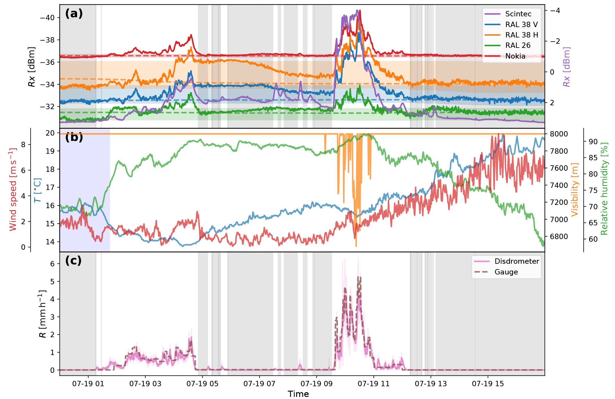
Figure 16 Time series of an event on 19 July 2015. (a) Received power levels at the detectors (solid lines) and reference levels (median over dry periods in a 24 h moving window: dashed lines). The 5th and 95th percentile power levels over dry periods in a 24 h moving window are indicated by the coloured shading. (b) Several atmospheric variables measured at the “Veenkampen” meteorological station: relative humidity, visibility, and ambient air temperature at 2 m, and wind speed indicated with blue, orange, green, and red lines, respectively. Periods with a negative net radiation flux at the surface are indicated with blue shading. (c) The spatial weighted average rainfall intensities derived from the disdrometers are indicated by the pink line, with the weighted standard deviation among the disdrometers displayed by the pink shaded area. The rainfall intensities derived from the tipping bucket gauge are indicated with the dashed line. Dry periods, as indicated by the disdrometers, are displayed by grey shaded areas.

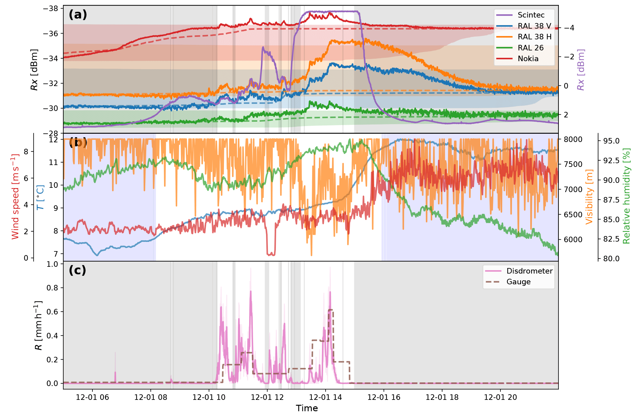
Figure 17 Time series of an event on 1 December 2015. (a) Received power levels at the detectors (solid lines) and reference levels (median over dry periods in a 24 h moving window: dashed lines). The 5th and 95th percentile of power levels over dry periods in a 24 h moving window are indicated by the coloured shading. (b) Several atmospheric variables measured at the “Veenkampen” meteorological station: relative humidity, visibility, and ambient air temperature at 2 m, and wind speed indicated with blue, orange, green, and red lines, respectively. Periods with a negative net radiation flux at the surface are indicated with blue shading. (c) The spatial weighted average rainfall intensities derived from the disdrometers are indicated by the pink line, with the weighted standard deviation among the disdrometers indicated with the pink shaded area. The rainfall intensities derived from the tipping bucket gauge are indicated with the dashed line. Dry periods, as determined with the disdrometers, are represented by grey shaded areas.

Figure 16 shows another example of a rain event. It can be seen that the link attenuation signals mimic the temporal dynamics in the rainfall. It can also be seen that the RAL 38 GHz link shows continued attenuation after the first rain event has stopped. One possible explanation could be because the antennas become wet themselves, which contributes extra to attenuation. However, the duration of the effect in this instance is almost 3 h, which is somewhat inconsistent with the results from Sect. 4.6, which suggests a duration in the order of 21 min. It is also inconsistent with some other events during this experiment when only a short attenuation period was observed after a precipitation event. Here as well, after the second rain shower, no lingering attenuation is observed. However, it is consistent with the findings of Schleiss et al. (2013). The Nokia link shows no lingering attenuation in both cases, which is consistent with the results from the wet antenna experiment. It is hard to specify why lingering attenuation effects occur after some rain events and not after others, but ambient conditions such as air humidity, temperature and wind speed might play a role here. The relative humidity hovers around 90 % after the first event, while it drops to 80 % directly after the second event. Concurrently, temperature increases from 14.5 to 18 ^∘C and wind speed increases from 1 to 6 m s⁻¹. It is even harder to specify why some antennas are much more affected by the phenomenon than others at a given time; however, the beading effect of the wet antenna with hydrophobic antenna cover might be related to this.

The examples given above have been simple cases where rain and other attenuating phenomena occur in an isolated fashion. These cases are important to be able to investigate and explain these phenomena. However, many times throughout the investigated period multiple phenomena have occurred simultaneously, which is a complicating factor for retrieval algorithms. Figure 17 provides an example of a complex event occurring on 1 December 2015. In this case, there is a simultaneous light drizzle and fog. Figure 17c shows that the disdrometers register rain intensities of below 1 mm h⁻¹ over a period of over 4 h. Despite the low intensity, the drizzle does produce attenuation of the links between 10:00 and 13:00, as can be seen in Fig. 17a. Fog rolls in at around 13:00 as evidenced by the time-lapse footage (not shown here) and substantiated by the increasing relative humidity and decreasing visibility as seen in Fig. 17b. From 13:00 till roughly 14:30 fog and drizzle occur simultaneously and both contribute to the attenuation. At 15:30 the fog has blown over or has dissipated. This is captured well by the Nokia link attenuation signal. The RAL link signals remain attenuated until 20:00. This could be due to the antenna covers still being wet. As was pointed out in Sect. 5.6, Due to bead formation, the hydrophobic antenna covers can stay wet much longer. Indeed, from 16:00 onwards, net radiation flux towards the surface is negative (indicated by the shading in Fig. 17b) and thus only wind drying can take place. The simultaneous occurrence of drizzle and fog could pose a problem for binary dew filtering algorithms such as the one proposed by Overeem et al. (2016b).

6 Conclusions

In this paper we have tested a straightforward rainfall retrieval algorithm applied to the microwave link measurements on the basis of a power-law relationship and compared the results with five disdrometers positioned along the path. This allows us to assess what the quality of a retrieval would be without taking into account the effect of other sources of attenuation. It is seen that there is a strong overestimation of rainfall intensities by the microwave links when compared to the disdrometers, when no corrections for the phenomena discussed in this paper are applied. The response of the link signals to liquid precipitation in terms of additive and multiplicative bias is of the same order of magnitude in both drizzle and heavier rainfall. This means that drizzle is much harder to quantify than heavier rainfall events because there is an additive bias of roughly 0.6 mm h⁻¹ in the Nokia link and roughly 2 mm h⁻¹ in the RAL links, i.e. of the same order of magnitude as typical rainfall intensities in drizzle.

There are significant differences in the accuracy of the rainfall retrieval between the two different makes of microwave links that we used, operating at the same frequency and polarization. In general, the commercial link has a less noisy and more unambiguously interpretable signal response than the dedicated research link. The latter overestimates the rainfall intensity more during pure rainfall events.

Unfortunately, there were only a few minor instances of snow and ice pellets occurring in the experimental area during the measurement period. Due to the limited amount of data no meaningful empirical conclusions can be drawn concerning the accuracy with which solid precipitation can be retrieved.

Of the three microwave links that we tested, two exhibited a significant dependence of received signal level on the ambient temperature. The received signal level of the research links was attenuated by −0.1 to −0.2 dB K⁻¹. The commercial link received signal level was not strongly attenuated by temperature, although a temperature dependence was found for a period where little other dynamic attenuating phenomena (rain, dew, etc.) were present. In this case, the (apparent) attenuation due to temperature was only −0.024 dB K⁻¹. Whether temperature dependence is a problem for rainfall retrieval that needs to be corrected for is thus dependent on the specific link hardware and not on the frequency (26 or 38 GHz) or polarization of operation.

We find attenuation due to fog or dew for all three microwave links. The peak magnitude of this attenuation in a typical event is 2 to 3 dB. The attenuation in the commercial link is slightly stronger than in the research links. The peak attenuation caused by fog or dew is of the same order of magnitude as a moderate rainfall event. If one would interpret such an event as rain the accumulated rainfall depth would be in the order of tens of millimetres. Therefore, it is important to correct for this phenomenon to obtain accurate rainfall data.

The use of a hydrophobic antenna cover should in principle reduce overestimation due to wet antennas. However, in practice, it also leads to bead formation which has adverse consequences. The beads take much longer to evaporate than a thin layer of water under similar circumstances, so after rainfall has stopped, or after dew conditions have subsided, the attenuation lingers much longer. More importantly, they make the magnitude of the attenuation during this drying-up period less predictable, because the configuration of the beads on the antennas is unpredictable. As such, we would tentatively recommend against the use of hydrophobic antenna covers for research links, although a more robust experiment might be needed to confirm this conclusion.

We also observed that in the typical urban environment temporary obstructions of the link path can lead to a link attenuation of several dB. Future research should be conducted to detect such sudden shifts in the baseline level and automatically correct for this.

Finally, we found that several of these phenomena can contribute to the apparent attenuation of the link signal concurrently. In particular, we show that light drizzle and fog can appear at the same time, which would lead to an overestimation of the rainfall intensity. Many current microwave link retrieval implementations currently rely on an a priori classification of a given time interval as either a rainy or dry period and assume the baseline signal level to be constant during a rainfall event. This is not sufficient for intervals where multiple effects play a role. Therefore, we believe the development of filtering methods which do not rely on an explicit binary classification should be explored.

In general, the use of two different microwave links operating at the same frequency along the same path during the same time (which should theoretically produce the same results) resulted in two remarkably different signal responses to rainfall and other attenuating phenomena. Therefore, we recommend that, when making use of data from commercial networks, note should be taken of the specific manufacturers and models the network is comprised of and the retrieval algorithm should be optimized for those link devices (i.e. by putting an example device in a test environment). This is especially relevant when parts of the network are supplied by different manufacturers. However, the remarkable stability of the Nokia link does demonstrate the value of commercially available microwave links for precise rainfall measurements when sampled at high frequencies.

We have demonstrated the effect of several complicating phenomena in typical microwave attenuation data for rainfall retrieval. The collected data from this experiment could be used to assess the effect of different sampling strategies used by commercial microwave links from cellular communication networks in operational settings. Moreover, the experimental data can also be used as a test dataset to improve existing algorithms (e.g. Overeem et al., 2016a) and devise corrections for the plethora of attenuating phenomena described in this paper.