the Creative Commons Attribution 4.0 License.
the Creative Commons Attribution 4.0 License.
 | 30 Oct 2018
Doppler W-band polarization diversity space-borne radar simulator for wind studies
Ranvir Dhillon
Anthony Illingworth
CloudSat observations are used in combination with collocated European Centre for Medium-Range Weather Forecasts (ECMWF) reanalysis to simulate space-borne W-band Doppler observations from slant-looking radars. The simulator also includes cross-polarization effects which are relevant if the Doppler velocities are derived from polarization diversity pulse pair correlation. A specific conically scanning radar configuration (WIVERN), recently proposed to the ESA-Earth Explorer 10 call that aims to provide global in-cloud winds for data assimilation, is analysed in detail in this study.
One hundred granules of CloudSat data are exploited to investigate the impact on Doppler velocity estimates from three specific effects: (1) non-uniform beam filling, (2) wind shear and (3) crosstalk between orthogonal polarization channels induced by hydrometeors and surface targets. Errors associated with non-uniform beam filling constitute the most important source of error and can account for almost 1 m s−1 standard deviation, but this can be reduced effectively to less than 0.5 m s−1 by adopting corrections based on estimates of vertical reflectivity gradients. Wind-shear-induced errors are generally much smaller (∼0.2 m s−1). A methodology for correcting these errors has been developed based on estimates of the vertical wind shear and the reflectivity gradient. Low signal-to-noise ratios lead to higher random errors (especially in winds) and therefore the correction (particularly the one related to the wind-shear-induced error) is less effective at low signal-to-noise ratio. Both errors can be underestimated in our model because the CloudSat data do not fully sample the spatial variability of the reflectivity fields, whereas the ECMWF reanalysis may have smoother velocity fields than in reality (e.g. they underestimate vertical wind shear).
The simulator allows for quantification of the average number of accurate measurements that could be gathered by the Doppler radar for each polar orbit, which is strongly impacted by the selection of the polarization diversity H−V pulse separation, Thv. For WIVERN a selection close to 20 µs (with a corresponding folding velocity equal to 40 m s−1) seems to achieve the right balance between maximizing the number of accurate wind measurements (exceeding 10 % of the time at any particular level in the mid-troposphere) and minimizing aliasing effects in the presence of high winds.
The study lays the foundation for future studies towards a thorough assessment of the performance of polar orbiting wide-swath W-band Doppler radars on a global scale. The next generation of scanning cloud radar systems and reanalyses with improved resolution will enable a full capture of the spatial variability of the cloud reflectivity and the in-cloud wind fields, thus refining the results of this study.
- Article
(5902 KB) - Full-text XML
- BibTeX
- EndNote


Observations of atmospheric 3-D winds and their monitoring on multiple temporal and spatial scales have been identified as a priority in the recent NASA Decadal Survey (The Decadal Survey, 2017). Large-scale winds are paramount in the transport of energy and water through the atmosphere and, together with vertical motions of convection, are the main driver in controlling water vapour transport around the globe. They are an essential element in the circulation of the atmosphere, in coupling clouds and the general circulation, in understanding the hydrological cycle and in untangling climate challenges (Bony et al., 2015).
Zeng et al. (2016) state that “it is important to avoid all-or-nothing strategies for 3-D wind vector measurements”, i.e. that progress can be achieved with observing strategies that are not comprehensive and are only effective in certain conditions (clear sky, cloudy, etc.) and may be capable of measuring only one or two components of the wind that complement each other. An integrated approach to active sensing (lidar, radar, scatterometer) and passive imagery or radiometry-based atmospheric motion vectors is therefore envisaged for improving global observations of winds in the future. In this synergistic approach, active sensors on LEO satellites could be used to calibrate observations from geostationary satellites that have excellent temporal coverage but are affected by large errors in assigning a height to the retrieved wind. Profiles of tropospheric winds currently have the highest priority (“the holy grail”) for all operational weather agencies. Doppler active sensors (lidars and radars) on LEO satellites which use atmospheric targets as wind tracers are unanimously credited to be the key instruments that achieve this priority. While an explorer/incubation mission of this type is recommended by NASA for the next decade (The Decadal Survey, 2017), the ESA Earth Explorer programme already has two missions in the pipeline aiming for this goal. The ESA Aeolus mission to be launched in mid-2018 (Stoffelen et al., 2005) will provide the first Doppler lidar measurements of the line-of-sight winds in clear air and thin ice clouds. It will be followed by the ESA-JAXA EarthCARE mission (launch planned for 2020, Illingworth et al., 2015) that will provide vertical velocities of cloud particles via a nadir-pointing Doppler W-band radar. For the first time sedimentation rates of ice crystals (Kollias et al., 2014) and convective up- and downdraughts (Battaglia et al., 2011) will be observed from space.
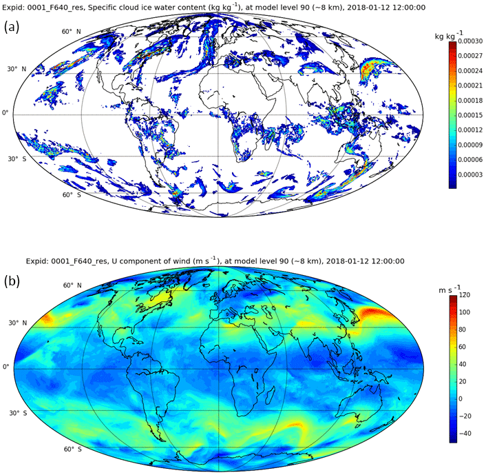
Figure 1Cloud ice water content (a) and ECMWF zonal winds (b) at a height of 8 km at noon on 2 January 2018. The data are plotted at a resolution of about 14 km. Ice water is only plotted when the mixing ratio exceeds 10−6 kg kg−1 or 10−3 g m−3 or a reflectivity of dBZ (Hogan et al., 2006). Plot courtesy of Michael Rennie, ECMWF.
However, none of these missions will be able to provide horizontal winds in deep cloud systems. McNally (2002) showed that “sensitive” areas in which observations have the largest potential to improve forecasts are often cloudy. The nexus between clouds and winds is revealed in Fig. 1, a snapshot of the global winds and ice water content (IWC) at a height of 8 km from the European Centre for Medium-Range Weather Forecasts (ECMWF) model for 12 noon on 12 January 2018. Particularly obvious are the high values of IWC and rapidly changing winds associated with the storm to the south of Japan, as is the case for other midlatitude depressions. Areas in which winds change rapidly are often associated with clouds, and only radars can penetrate such areas.
Recent European Space Agency (ESA)-funded studies suggested addressing this wind observational gap by using W-band radars – ideal for their high sensitivity and narrow beamwidths – with scanning and Doppler capabilities. Both a stereoradar and a conically scanning configuration have been proposed (Battaglia and Kollias, 2014a; Illingworth et al., 2018a). The former investigates the link between microphysical and dynamical structures of cloud systems, including convective systems, while the latter, known as WInd VElocity Radar Nephoscope (WIVERN), aims to provide global in-cloud winds for data assimilation and has now been proposed to the ESA Earth Explorer 10 call (Illingworth et al., 2018b). By conically scanning an 800 km wide ground track, the radar allows the measurement of large-scale winds associated with long-lived systems to be assimilated into weather forecast models with daily coverage at midlatitudes.
The commonalities of both systems are as follows:
-
They look/scan at a slant view (incidence angles in the range between 40 to 50∘) in order to capture horizontal winds.
-
They adopt polarization diversity to overcome the range-Doppler dilemma and to cope with the short decorrelation times associated with the Doppler fading inherent to millimetre Doppler radars on fast-moving low Earth orbiting satellites (Kollias et al., 2014; Tanelli et al., 2002).
-
They require large antennas to achieve narrow (∘) antenna beamwidth and thus to optimize the Doppler quality.
By focusing on slant-looking Doppler radars adopting polarization diversity, this study aims to define a simulation framework which enables the assessment of radar performance on a global scale.
Doppler velocity accuracy requirements depend on the application, but the WMO requirement for assimilating winds is to have errors lower than 2 m s−1 at a horizontal sampling of 50 km and a vertical resolution of 1 km or better (see Illingworth et al., 2018a for a thorough discussion of wind user requirements). Noticeably Horanyi et al. (2014) state that assimilating winds with biases of 1–2 m s−1 can actually degrade the forecast. It is therefore important to assess the accuracy and precision of Doppler velocities for future space-borne wind-observing radars. There are several sources of uncertainty associated with polarization diversity Doppler measurements from space, such as errors linked to non-uniform beam filling (NUBF) (Tanelli et al., 2002) coexisting with or without wind shear, crosstalk between the H and V returns (Illingworth et al., 2018a; Pazmany et al., 1999; Wolde et al., 2018), clutter contamination, aliasing (Battaglia et al., 2013; Sy et al., 2013), mispointing (Battaglia and Kollias, 2014b; Tanelli et al., 2005), multiple scattering (Battaglia and Tanelli, 2011) and errors related to the Doppler estimators in the pulse-pair processing. The uncertainties associated with the pulse-pair processing are very well characterized: they depend on the signal-to-noise ratio (SNR), the radar Doppler spectral width, and the number of averaged samples (Battaglia et al., 2013; Doviak and Zrnić, 1993; Illingworth et al., 2018a). The other errors are more complicated and are generally assessed via simulations of cloud-resolving model scenes (Battaglia et al., 2013; Leinonen et al., 2015). In other cases, in order to avoid the uncertainties associated with transforming bulk microphysical properties to radar reflectivities, ground-based (Burns et al., 2016; Kollias et al., 2014) or aircraft (Sy et al., 2013, 2014) observations at the same radar frequency are exploited, with the advantage of reproducing naturally observed fields of reflectivity, together with their spatial variability. On the other hand, such observations are seldom representative of the global scale. In addition, only Battaglia et al. (2013) and Battaglia and Kollias (2014a) have addressed issues related to polarization diversity in a simulation framework.
In this study we exploit CloudSat W-band radar observations (Tanelli et al., 2008) in combination with collocated ECMWF wind reanalysis to simulate space-borne W-band Doppler radar observations from off-nadir scanning radars. The simulator also includes cross-polarization induced by atmospheric targets in order to assess its impact on Doppler polarization diversity pulse-pair estimates. The proposed simulation framework can therefore enable an error budget assessment on a global scale for a satellite mission adopting a sun-synchronous orbit similar to CloudSat. Section 2 provides information about the data sets that have been used while Sect. 3 describes the Doppler radar simulator and its application to the case study of Hurricane Igor. In Sect. 4 ∼100 orbits of CloudSat data are exploited to characterize the performance of a W-band Doppler system on a global scale. Conclusions and future work are presented in Sect. 5.
In order to simulate realistic scenes for assessing the capabilities of future space-borne W-band Doppler radars, two ingredients are needed: (1) W-band reflectivity profiles through a variety of cloud regimes with spatial resolutions comparable to or better than those to be simulated and capable of representing the natural variability, and (2) wind profiles for the whole troposphere. In this work the former are taken from the CloudSat W-band radar, and the latter are extracted from ECMWF products.
2.1 CloudSat products
The CloudSat 94 GHz (3.2 mm) Cloud Profiling Radar (CPR) measures reflectivities from cloud- and precipitation-sized particles at a vertical resolution of 480 m for a cross-track/along-track horizontal footprint of 1.5 km ×2.5 km (Stephens et al., 2008). The radar has been collecting data on a polar sun-synchronous orbit since its launch in 2006 (Tanelli et al., 2008). This study makes use of different Level 2 CloudSat data products: the 2B-GEOPROF (Mace et al., 2007), the 2B-CLDCLASS-LIDAR (Sassen et al., 2008) and the 2C-RAIN-PROFILE (Haynes et al., 2009) (more details at http://www.cloudsat.cira.colostate.edu/, last access: 19 October 2018).
2.2 ECMWF product
The European Centre for Medium-Range Weather Forecasts (ECMWF) maintains an archive of meteorological and air-quality data – covering a wide range of parameters including, for example, gas and pollutant concentrations, precipitation measurements and wind values – central to its core mission of producing numerical weather forecasts and monitoring the Earth system (https://www.ecmwf.int/, last access: 19 October 2018).
For the study covered here, ECMWF global wind fields (u and v components) are used at a temporal resolution of 6 h and latitude and longitude resolutions of 0.1∘. The wind fields are provided at 25 pressure levels ranging from 1 to 1000 hPa. They are collocated with the CloudSat measurements by selecting the nearest ECMWF grid point (latitude and longitude) to the CloudSat position and by temporally interpolating to each CloudSat profile time stamp between the two closest ECMWF time stamps.
3.1 Radar configuration
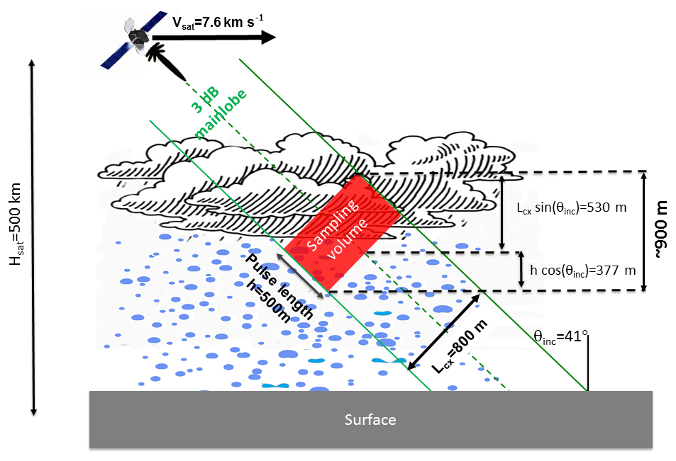
The radar configuration that will be used throughout this paper is the one depicted in Fig. 2. The radar specifications are detailed in Table 1. The configuration corresponds to the one proposed for the WIVERN mission (which involves a conically scanning system) when the antenna is looking in the same direction as the spacecraft motion (Illingworth et al., 2018a, b) and is very similar to the one proposed in Battaglia and Kollias (2014a). Therefore, we will refer to it as the WIVERN forward configuration. The antenna pattern is assumed Gaussian with a two-way gain equal to the following:
where G0 is the antenna gain in the boresight direction, θ is the antenna polar angle with respect to the boresight and θ3 dB is the antenna 3 dB beamwidth. The radar reflectivity and Doppler velocity are computed as follows:
where V is the backscattering volume (red box in Fig. 2), vr is the wind velocity along the line of sight and Zm is the measured reflectivity (generally variable within the backscattering volume). Since CloudSat only provides a 2-D curtain through cloud systems, the integral in Eq. (2) is reduced to a 2-D integral that can be performed in polar coordinates.
Table 1Specifics of the radar for the simulation. The configuration adopted here is the one proposed for WIVERN in a recent ESA Earth Explorer 10 call.
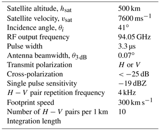

Figure 3(a) CloudSat radar vertical reflectivity profile at W-band for overpass of Atlantic Hurricane Igor on 16 September 2010 between 17:13 and 17:28 UTC (corresponding to along-track distance of 2200 km). The ECMWF line-of-sight winds projected onto the CloudSat curtain are plotted as arrows. (b) Contour plot of ECMWF line-of-sight winds. The reflectivity data are provided at CloudSat resolution (1.1 km horizontal, 0.5 km vertical), whereas the ECMWF winds are at 0.1∘ resolution (∼10 km). For presentation purposes, only winds every 10 km along the curtain and every 700 m in the vertical are shown (a).
3.2 Case study: Hurricane Igor
The simulator rationale is demonstrated for a case study based on a CloudSat overpass over Hurricane Igor. Hurricane Igor originated from a broad area of low pressure that moved off the Cabo Verde islands on 6 September 2010. It subsequently developed into a tropical depression on September 8 and reached Category 4 status on 12 September with winds peaking at 70 m s−1. CloudSat in ascending orbit overpassed to the east of the storm centre on 16 September1 when Igor had gradually started weakening. Figure 3 shows the CloudSat radar vertical reflectivity profile derived from the 2B-GEOPROF product across the whole hurricane: the system extends for about 2200 km horizontally with clouds towering to almost 16 km. Some deep convection and heavy precipitation are clearly present close to the centre of the plot corresponding to the eye wall: attenuation is so strong that even the surface signal is completely attenuated. Some deep isolated convective towers are present to the south (left side of the panel) in association with the spiral bands. The cirrus canopy stretches across most of the overpass, but it is much taller in the southern part.
The wind field of course varies appreciably over the scene, and this is exemplified by the characteristic change in the line-of-sight velocity component that occurs across the hurricane (indicated by the arrows in Fig. 3). This line-of-sight component, which is determined by combining ECMWF and CloudSat data, varies significantly over the horizontal extent of the hurricane, with values ranging from approximately −10 to +30 m s−1 at along-track distances of about 0 and 1000 km respectively (Fig. 3). The region with the highest wind magnitudes is associated with the upper levels in the central tallest part of the system.
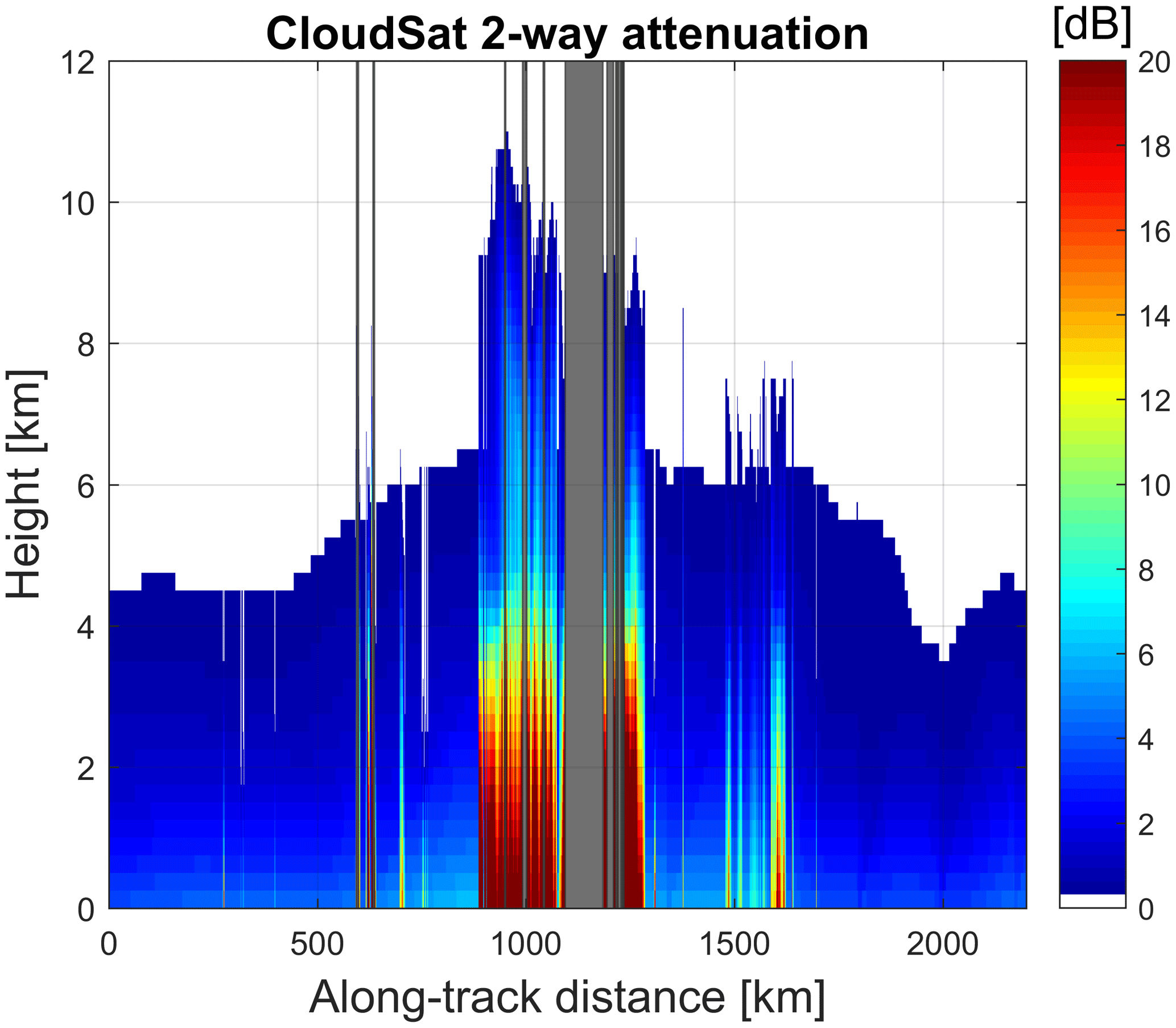
Figure 4Two-way attenuation as retrieved in the 2C-RAIN product for the scene shown in Fig. 3. Grey bands correspond to profiles for which the retrieval in the 2C-RAIN product is not applicable. Data are provided at CloudSat resolution (1.1 km horizontal, 0.5 km vertical).
The 2C-RAIN product reconstructs vertical profiles of attenuation (see Fig. 4) and of effective reflectivities based on an optimal estimation framework. The retrieval is not applicable in regions of strong convection in the presence of multiple scattering and high attenuation (Battaglia et al., 2011; Matrosov et al., 2008), where no convergence of the algorithm is obtained. These regions are marked by the grey stripes in Fig. 4. No reconstruction of simulated profiles will be attempted in such regions. Note that in regions filled with precipitation the two-way path-integrated attenuation can exceed 30 dB.
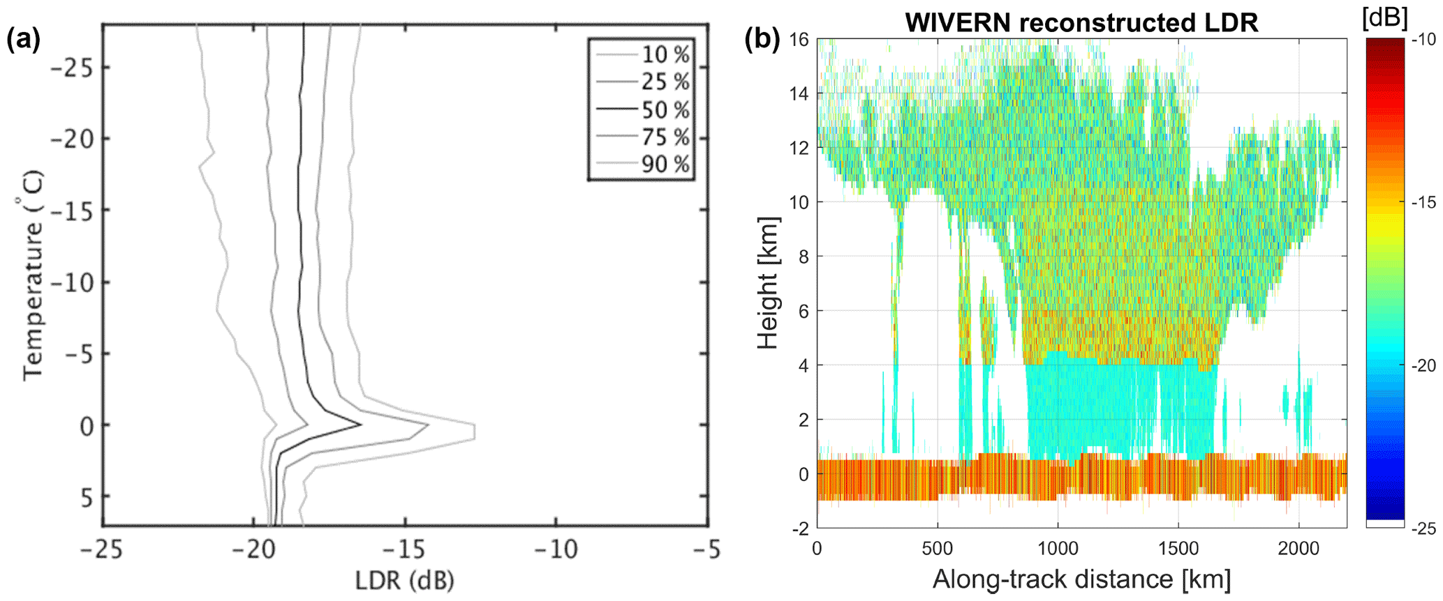
Figure 5(a) Climatological observations of W-band LDR at the Chilbolton Observatory for an elevation angle of 45∘ (courtesy of John Nicol, University of Reading). (b) Simulated LDR for the scene shown in Fig. 3 at CloudSat resolution (1.1 km horizontal, 0.5 km vertical).
To simulate a Doppler radar with polarization diversity, linear depolarization ratio (LDR) profiles are also needed (see discussion later in Sect. 3.3.3). A crude LDR is reconstructed based on climatological observations of LDR at the Chilbolton Observatory (see left panel in Fig. 5). Data were collected during June and July 2017 at 45∘ elevation with the W-band Galileo polarimetric radar. Different hydrometeors (as derived from the 2B-CLDCLASS-LIDAR product) are assigned LDR values drawn from a normal distribution with 0.5, 1.5, 2 and 1.5 dB standard deviation and mean values of −19, −18, −16 and −17 dB for rain, ice crystals, melting particles and the mixed-phase region respectively. Surface LDR are assumed to be normally distributed around −14 and −7 dB for sea and land respectively with 2 dB standard deviation (Battaglia et al., 2017).
To produce realistic simulations of slant-looking radars, two aspects must be accounted for.
-
The slant-viewing geometry (with an increased cumulative attenuation compared to nadir-looking radar) and the appropriate antenna pattern (Eq. 1) must be accounted for. This is possible because unattenuated reflectivities and attenuation estimates are available from the 2C-RAIN product so that the measured reflectivity (term Zm appearing in the integral of Eq. 2) can be properly computed for each direction of the antenna pattern; the integration over the backscattering volume is carried out at the initial 1.1 km integration length of CloudSat. Further along-track averaging is performed later (e.g. resolution of winds for data assimilation is about 20 km).
-
The ground clutter must be significantly reduced, especially over ocean. In Fig. 3 the ocean surface return is very strong because CloudSat is almost nadir looking. On the other hand, in the configuration shown in Fig. 2, the surface clutter will be significantly lower. Recent airborne studies at 94 GHz and WIVERN incidence angles (Battaglia et al., 2017) have established the natural variability of the normalized radar surface backscattering, σ0. Accordingly, in this study, sea (land) surface σ0 values have been assumed to be normally distributed around −25 dB (−8 dB) with standard deviation equal to 5 dB (4 dB).

Figure 6Reconstructed reflectivity (a) and line-of-sight Doppler velocities (b) simulated for a system with the specifics listed in Table 1 and starting from the CloudSat scene illustrated in Fig. 3. The regions shaded in grey correspond to areas in which no reconstruction of the reflectivity profile is possible due to severe attenuation or multiple scattering. Reflectivities and Doppler velocities are produced with a 20 km integration length for a total of 200 H−V pairs with a Thv=20 µs (which corresponds to a Nyquist velocity of 40 ms−1).
The result of the simulator is shown in Fig. 6. Note that the grey stripes correspond to the regions in which no attenuation correction is deemed possible, which go from approximately 2 km above the freezing level to the ground, corresponding to the grey bands for which the 2C-RAIN product is not applicable (grey stripes in Fig. 4). Because of the slant geometry and the 20 km integration the grey bands are now wider than for Fig. 4.
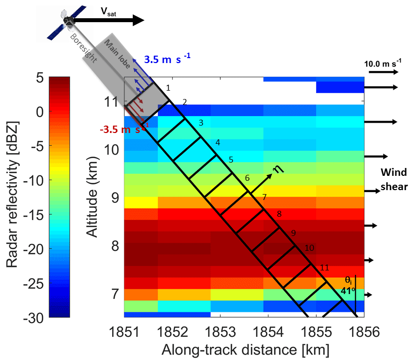
Figure 7Diagram explaining Doppler velocity errors introduced by NUBF. The reflectivity profiles are extracted from Hurricane Igor (ice clouds corresponding to the red arrow in the left panel of Fig. 3). The black rectangles represent the backscattering volumes associated with the 3 dB antenna main lobe.
3.3 Errors
The simulation framework is ideal for properly assessing Doppler (reflectivity-weighted) line-of-sight velocity estimate () errors on a global scale. Here, we will focus our analysis on three different sources of errors, which are related to the spatial structure of the wind and of the reflectivity fields: errors due to NUBF, to the presence of wind shear and to the crosstalk between channels induced by atmospheric targets when adopting polarization diversity.
3.3.1 Non uniform beam filling: satellite motion-induced biases
For a fast-moving space-borne Doppler radar, radar reflectivity gradients within the radar sampling volume can introduce a significant source of error in Doppler velocity estimates (Tanelli et al., 2002). In fact, the component of the satellite velocity along the line of sight presents a shear across the backscattering volume. In Fig. 7 the configuration adopted in Fig. 2 is used to illuminate the small radar volume identified by the red arrow in Fig. 3. If the frequency Doppler shift and the associated Doppler velocity corresponding to the antenna boresight direction are perfectly compensated for and set to zero, then the forward (backward) part of the backscattering volume appears to move upward (downward) as illustrated by the blue (red) arrows. Across the 3 dB footprint size, this velocity ranges from −3.5 to +3.5 m s−1. When coupled with a reflectivity gradient, this satellite-motion-induced velocity shear can produce a bias. For instance, for the backscattering volumes labelled as 11 (6) in Fig. 7, there is a positive (negative) reflectivity vertical gradient which will produce an upward (downward) bias.
The combined CloudSat and ECMWF data sets have been exploited to quantify the effect of NUBF biases as experienced by a satellite orbiting in a polar sun-synchronous orbit. An estimate of these biases is obtained by considering the difference between m s−1] corrected for satellite motion and , where the satellite velocity is set to 0 m s−1. The NUBF-induced bias corresponding to the scene of Hurricane Igor depicted in Fig. 6 is shown in Fig. 8. The main feature is represented by upward biases at the cloud top and downward biases at the cloud base, both of which are up to several m s−1.
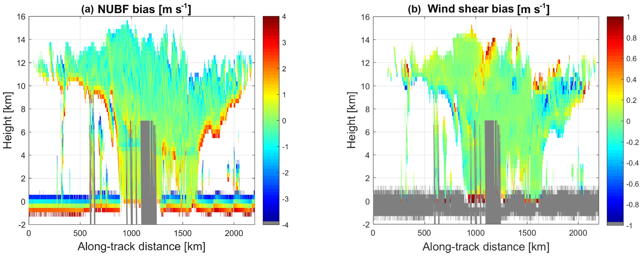
Figure 8NUBF-induced (a) and wind-shear-induced (b) errors for the Hurricane Igor scene shown in Fig. 6. Most of the biases are near the cloud edge; widespread biases of ∼1 m s−1 must be avoided.
For nadir-pointing radars, notional studies demonstrated that such biases can be mitigated by estimating the along-track reflectivity gradient because NUBF-induced biases are expected to be linearly proportional to such reflectivity gradients (Kollias et al., 2014; Schutgens, 2008; Sy et al., 2013). Similarly, in a slant-looking geometry the relevant gradients are those along the direction orthogonal to the boresight and lying in the plane containing the satellite velocity and the antenna boresight direction (η direction in Fig. 7, Battaglia and Kollias, 2014a). If conically scanning systems are considered it will be more challenging to retrieve the Z gradients along such directions for all scanning angles; moreover it is expected that such gradients will be affected by the vertical reflectivity gradients, which are typically larger than horizontal gradients. In the presence of a vertical reflectivity gradient, ∇zZ (in dB m−1), if the reflectivity field can be approximated to vary linearly within the backscattering volume, then the bias introduced by the satellite motion is equal to the following (Battaglia and Kollias, 2014a; Sy et al., 2013):
where r is the range from the radar. For instance, for the WIVERN configuration (Table 1) this corresponds to a bias of 0.077 m s−1 per dB km−1.
3.3.2 Wind shear
Similarly, biases in the radar-derived winds may arise when there is a vertical wind shear (see arrows on the right-hand side of Fig. 7) coupled with a large vertical gradient of radar reflectivity across the radar backscattering volume. An estimate of these biases is obtained by considering the difference between and , where the latter is the line-of-sight velocity estimate averaged over the antenna pattern but not reflectivity weighted, i.e.
For the Hurricane Igor case study, the results are shown in the right panel of Fig. 8: wind-shear-induced biases are generally smaller than NUBF-induced biases with amplitudes up to 1 m s−1 and confined to the areas at the edge of clouds characterized by large wind shear and vertical reflectivity gradients.
Since the vertical wind shear is generally considerably larger than the horizontal one, under the assumption that the reflectivity and wind fields can be approximated to vary linearly within the backscattering volume, the bias due to wind shear can be approximated as follows:
where ∇zZ and ∇zv are the reflectivity and wind vertical gradients expressed in dB m−1 and in s−1. For instance for the WIVERN configuration (Table 1) this corresponds to a bias of 0.37 m s−1 per dB km−1 for a wind shear of 0.01 s−1. The reflectivity gradients and wind shear along the vertical direction can be inferred from adjacent gates and therefore a correction can be attempted.
3.3.3 Crosstalk
Doppler systems adopting polarization diversity assume that the V and H waves propagate and scatter independently without any interference. In reality the effect of cross-polarization is to produce an interference signal in each co-polar channel depending on the temporal shift between the H and V pair and the strength of the cross-polar power. Such interferences appear in the co-polar channels as “ghost echoes”. Crosstalk between the two polarizations can occur either at the hardware level or can be induced by propagation and/or backscattering in the atmosphere. While the former is typically reduced to values lower than −25 dB, the latter can be important and is characterized by the LDR. The phases of ghost echoes are incoherent with respect to the echoes of interest so do not bias the velocity estimates, but increase their random error as a function of the signal-to-ghost ratio (Pazmany et al., 1999; Wolde et al., 2018). This quantity depends on the reflectivity profile structure and on Thv, the time separation between the H− and V− polarized pulses. The full theory is reviewed in depth in Wolde et al. (2018), Eqs. (6)–(11). An example of the line-of-sight measured Doppler velocity for a Thv=20 µs is shown in the right panel of Fig. 6 for the WIVERN forward configuration. The Doppler winds compare well with those from ECMWF, shown in the right panel of Fig. 3. Note how the measurements become increasingly noisy when moving towards lower SNRs.
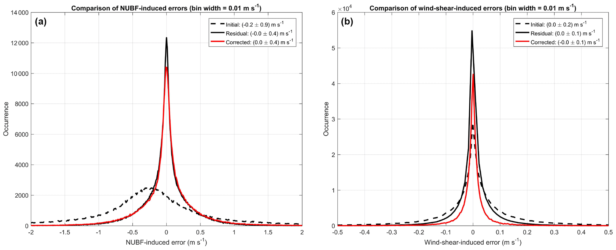
Figure 9(a) Distribution of 8-day CloudSat data set NUBF-induced (wind-shear-induced) errors. Black dashed line is initial errors, black solid line is errors after correction with perfect measurements, red line is errors after correction with noisy measurements. A Thv=20 µs and a spectral Doppler width of 4 m s−1 have been assumed when including noise.
Eight days of CloudSat data, from 1 to 8 September 2010, have been used to obtain simulated residual errors, defined as the difference between the actual velocity biases and the velocity corrections obtained using the formulae given above. The data set comprises 94 granules and therefore covers a variety of cloud types with a multitude of characteristics. The CloudSat data granules used for this study were chosen based on whether data files corresponding to the four relevant CloudSat data products (2B-GEOPROF, 2B-CLDCLASS, 2C-RAIN-PROFILE and ECMWF-AUX) were all present simultaneously.
4.1 NUBF and wind shear errors and corrections
The technique demonstrated for Hurricane Igor in Sect. 3.2 has been applied to the whole data set. First the magnitudes of the errors induced by NUBF and wind shear are evaluated; e.g. the wind-shear-induced biases are obtained by subtracting the ECMWF (antenna-weighted) winds from the reflectivity-weighted winds. The black dashed lines in Fig. 9 show the distribution for the NUBF-induced (left) and wind-shear-induced error (right), with the former significantly larger (standard deviation of 0.9 m s−1 vs. 0.2 m s−1) compared to the latter and slightly biased (−0.30 m s−1). This bias is due to the fact that the average reflectivity vertical gradient (when all heights are considered) is slightly negative. Note that this bias will cancel out if a backward look is also adopted (as for the conically scanning WIVERN).
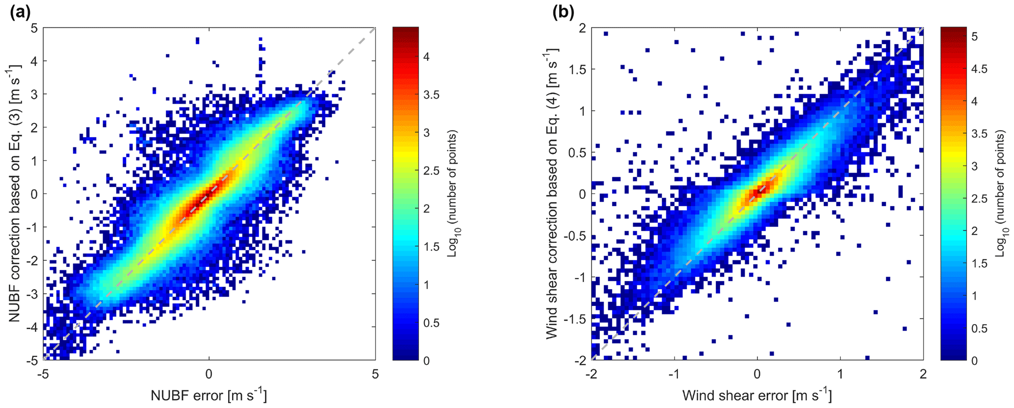
Since CloudSat reflectivity and ECMWF wind fields are defined at coarse horizontal scales, the simulation may not account for the full variability inside the backscattering volume; thus the errors may be underestimated. Second, the quality of the corrections derived from the formulae given by Eqs. (3)–(4) is tested by comparing NUBF-induced and wind-shear-induced errors with their corresponding corrections (left and right panels of Fig. 10, which are occurrence density plots with the colours corresponding to log10 N, where N is the number of points in the bin). So far, the reflectivity and Doppler velocity measurements have been assumed to be free of noise. Clearly the corrections to NUBF- and wind-shear-induced errors appear to match the actual NUBF- and wind-shear-induced biases very well. This implies that a very accurate wind field can be constructed from the reflectivity-weighted winds with standard deviations reduced to 0.4 and 0.1 m s−1 (see solid black lines in Fig. 9).
However, real reflectivity and Doppler velocity data are subject to noise, and the impact will depend on the SNR value. In the selected configuration a single-pulse SNR of 0 dB corresponds to an echo of −19 dBZ. For instance, in terms of velocity errors, for a 20 km along-track integration (i.e. 200 pulse pairs) the errors due to the pulse pair processing are of the order of 1.5 m s−1 at 0 SNR (see Fig. 3 in Illingworth et al., 2018b).
In order to ascertain whether accurate wind fields can be retrieved from the Doppler radar data, it is necessary to examine how well the vertical reflectivity and Doppler velocity gradients, which enter Eqs. (3)–(4), can be obtained in the presence of varying levels of noise. The effectiveness of the wind corrections therefore has been studied by injecting noise into the reflectivities and Doppler velocity fields. This noise has been assumed to take the form of normally distributed fluctuations with magnitudes that are determined by the actual SNR, the spectral width of the Doppler spectrum and the selected Thv (according to formula 6 in Hogan et al., 2004 for the reflectivity noise and formula 15 in Pazmany et al., 1999 for the Doppler velocity noise). Since the addition of noise causes large variations in reflectivity and wind gradients obtained from noisy data, efforts have been made to mitigate any consequent negative effects by applying a running mean to the data along the line of sight (averaging over three range bins) with the intent of smoothing them before the gradients are computed. The solid red lines in Fig. 9 show the distribution of the errors associated with NUBF (left) and wind shear (right) once the corrections described by Eqs. (3)–(4) are applied based on velocity and reflectivity gradients estimated after the injection of noise into reflectivities and Doppler velocities. No range averaging is performed. Note that the wind-shear-induced correction (right panel) is applied only for SNR ≥ 16 dB (see discussion here below).
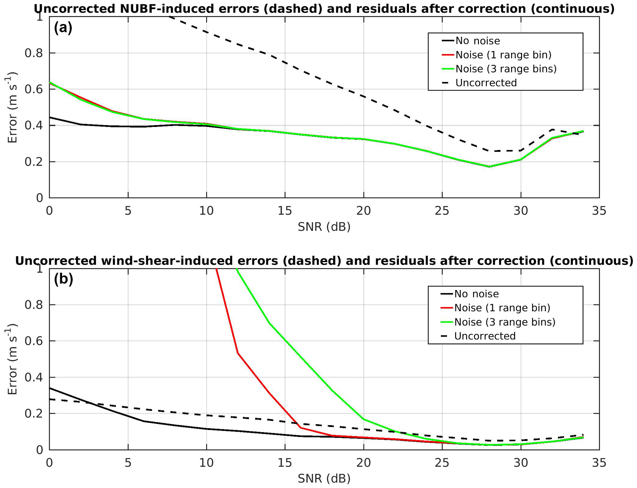
Figure 11The NUBF-induced (a) and wind-shear-induced (b) root mean square errors as a function of the SNR computed (1) without noise (black solid lines), (2) with added noise and estimating gradients from variables at the native range resolution of 500 m (red solid lines) and (3) with added noise and estimating gradients from variables computed from running averages over three range bins (green solid lines). The statistics are built from 8 days of CloudSat data. Initial uncorrected errors are plotted as black dashed lines.
The errors in the wind estimates due to the NUBF-induced and wind-shear-induced effects are shown in Fig. 11 (top and bottom panels) as a function of the SNR. The horizontal axis shows the signal-to-noise ratio, with 0 dB corresponding to a reflectivity of −19 dBZ, and the vertical axis shows the root mean square errors (RMSEs) computed with reference to the “true wind” (i.e. the one that would be measured without reflectivity gradients). The initial RMSEs where the corrections given by Eqs. (3) and (4) have not been applied are shown as black dashed lines. The RMSEs are recalculated after the corrections are applied. Three conditions are examined. The corrections are applied: (1) without adding any noise to the measurements (black solid line); (2) by adding noise to the measurements as expected for the WIVERN system (red solid lines); (3) by adding noise and estimating gradients after applying running averages over three range bins of ∼0.5 km (green solid lines).
Clearly the corrections for NUBF-induced RSMEs vary little with SNR. Even without range averaging, the correction based on Eq. (3) produces results similar to those for the perfect correction without any noise (black solid line) and is only slightly worse for SNR <10 dB. It is worth applying the correction as the RMSEs are reduced significantly from their initial value (black dashed line). There is an increase in the NUBF-induced RMSEs for SNR above about 28 dB, although the error remains below 0.4 m−1. This is caused by a tendency for data to deviate from the one-to-one line (grey dashed line in Fig. 10) at the highest SNR values, thus suggesting that at higher reflectivities the correction becomes less linear. As a result, the correction given by Eq. (3) may be less effective at these highest SNR values. Horanyi et al. (2014) show that the bias must be less than 1 m s−1 but that higher random errors are acceptable: the errors documented here appear to largely fulfil such conditions.
For the case of wind-shear-induced RMSEs, the correction clearly becomes more effective only at high SNR in the presence of noise, with the RMSEs computed in such condition approaching those computed without noise only for SNR ∼ 20 dB (red vs. black line). For SNR <20 dB, there is a significant deviation between the noise and no-noise cases. The initial wind-shear-induced error computed without any correction (dashed line) is very small for all SNR. While the correction would further reduce the RMSE in the presence of perfect measurements with no noise (black line), the contrary is true in the presence of noise for all values of SNR <20 dB (red solid vs. black dashed line). This increase in the wind-shear-induced RMSE is caused by noise-induced variations in the velocity gradient. These noise-induced changes render the correction ineffective at lower SNR. Interestingly, averaging over three vertical range bins makes the correction worse (green solid line), with the corrected value only approaching the no-noise value at about 25 dB SNR. In contrast to the case for NUBF-induced errors, where the correction produces notable improvement for all SNR values, the correction for wind-shear-induced effects will reduce the error significantly only if it is applied for SNR >18 dB.

Figure 12The fraction of profiles (including cloudy and non-cloudy situations) from which winds at a given height can be derived with an accuracy of 2 m s−1 for various Thv values for high latitudes (a), midlatitudes (b) and tropical (c) oceanic conditions. Dashed (continuous) lines correspond to results when the ghosts are (are not) accounted for. A WIVERN forward configuration has been assumed (see Table 1) with an along-track integration length of 20 km. The WIVERN profiles have been reconstructed from CloudSat profiles over ocean with LDR and clutter signals reconstructed based on airborne observations of ocean surface returns.
4.2 Crosstalk errors and optimal Thv selection
Simulations of Doppler velocities have been generated using Thv values ranging from 5 to 40 µs, taking into account the SNR and the strengths of the ghost echoes for a 20 km along-track integration. The fraction of profiles for which a WIVERN forward configuration is expected to produce winds with accuracy better than 2 m s−1 is presented in Fig. 12 for high latitudes (top), midlatitudes (middle) and tropical (bottom panel) oceanic conditions. Dashed (continuous) lines correspond to results when the ghosts are (are not) accounted for. Clearly, the ghosts only marginally reduce the number of WIVERN measurements with accuracy better than 2 m−1. Specifically, the number of measurements with high accuracy is reduced by 1.8 %, 0.9 % and 0.3 % for Thv of 5, 20 and 40 µs respectively.
The fraction is much lower for the 5 µs Thv values because at this pair separation a small noise in the phase maps onto a large velocity error. Overall, Fig. 12 shows that in the mid-troposphere (3–8 km) WIVERN forward would provide a useful measurement of 10 % of the observation time, but this is expected to be significantly reduced over land at heights around 2 and around 4 km, where the bright land surfaces produce ghost echoes for Thv of 20 and 40 µs.
The selection of an optimal Thv certainly accounts for the result produced in Fig. 12, but other factors must also be considered:
-
Aliasing must be avoided. A Thv=20 µs corresponding to a Nyquist velocity vN∼40 m s−1 is certainly advantageous compared to a Thv=40 µs corresponding to a vN∼20 m s−1, when winds in extreme weather events are sought after.
-
Winds in the mid-troposphere are considered to be more important than winds in the lower troposphere. This is because there is a lack of winds in the middle troposphere (see Fig. 9 in Illingworth et al., 2018b) and because winds in the lower troposphere are more affected by boundary layer dynamics (which are less long-lived and therefore more difficult to assimilate). As a result it is preferable to have the surface ghosts as close to the surface as possible. Here only sea surfaces have been considered; land surfaces are much brighter (Battaglia et al., 2017) and therefore surface ghosts will play a more notable role. Again, this favours smaller Thv, e.g. Thv=20 µs (ghost layer centred at 2.2 km) vs. 40 µs (ghost layer centred at 4.5 km).
-
In the presence of large turbulence the Doppler spectral width can increase and greatly exceed the value predicted by accounting for the satellite motion only (Battaglia and Kollias, 2014a). This decreases the coherency time of the medium and, as a consequence, the optimal Thv value that minimizes the noise error is also reduced (see Fig. 8 in Battaglia and Kollias, 2014a).
CloudSat observations and Level 2 products have been used in combination with collocated ECMWF wind reanalysis to simulate space-borne oblique-viewing W-band Doppler observations for radars adopting polarization diversity, which have been recently proposed within the Earth Observation programmes of various space agencies. A specific radar configuration (the WIVERN; see Table 1), recently proposed for the ESA-Earth Explorer 10 call, is analysed in detail in this study. The simulator capitalizes on the fact that the CloudSat W-band Cloud Profiling Radar is in a polar orbit and therefore provides realistic global patterns of the radar reflectivity spatial variability at the W-band frequency range (and, when combined with ECMWF-winds, of how such patterns covary with the wind field), which are key drivers for establishing the performance of a W-band Doppler system on a global scale. The simulator is particularly suited for assessing the relevance of non-uniform beam filling and wind-shear-driven errors and of the effectiveness of their corrections based on the estimates of vertical gradients of the reflectivity and wind fields.
For data assimilation, properly quantified random wind errors are generally acceptable, but biases larger than 1 ms−1 cannot be tolerated. Our testing data set based on roughly 100 CloudSat granules shows that for an instrument looking at 41∘ slant angle and for a 20 km integration, both wind shear and NUBF introduce almost unbiased errors (biases of −0.3 and 0 m s−1) with standard deviations of the order of 0.9 and 0.2 m s−1. Such errors can be reduced if vertical gradients of reflectivity and of the wind can be estimated via Eqs. (3)–(4). If vertical gradients are perfectly estimated then the residuals in the Doppler velocities are unbiased and their standard deviations can be reduced to 0.2 and 0.1 m s−1. Practically, the corrections for both NUBF-induced and wind-shear-induced errors are effective in producing unbiased velocities (and perform at their best with SNR >10 dB and SNR >20 dB respectively).
The simulator also allows the quantification of the average number of accurate measurements that could potentially be gathered by the Doppler radar for each orbit. This is strongly impacted by the selection of the polarization diversity H−V pulse separation, Thv. For the WIVERN slant configuration a selection close to 20 µs seems to achieve the right balance between maximizing the number of accurate wind measurements (exceeding 10 % in the mid-troposphere) and minimizing aliasing effects in the presence of high winds. The presence of crosstalk only marginally reduces the region of measurements with high accuracy.
This study represents the first step towards a more sophisticated development of end-to-end simulators for space-borne oblique-viewing Doppler radars adopting polarization diversity. Further work could improve the simulator along the following guidelines.
-
The CloudSat radar only provides a 2-D curtain and thus does not capture the full 3-D structure of clouds. Moreover its vertical (500 m) and horizontal (1.4×1.7 km2) resolutions (Stephens et al., 2008) are not optimal for fully characterizing the spatial variability within the scattering volumes envisaged for future space-borne W-band Doppler radars. Future scanning radar missions will be able to provide 3-D structures of clouds (e.g. Durden et al., 2016) and are expected to be launched in the next decade (The Decadal Survey, 2017). In the meantime, cloud downscaling algorithms and stochastic models such as those proposed, e.g. in Barker et al. (2011); Venema et al. (2010) could be applied to the CloudSat data set in order to mimic the natural variability on smaller scales.
-
The effective reflectivity is retrieved for CloudSat profiles only over ocean, for which an estimate of the path-integrated attenuation is possible via the surface reference technique (Haynes et al., 2009). The analysis conducted in this paper is therefore limited to ocean cases only. The EarthCARE Cloud Profiling Radar, expected to launch in 2020 (Illingworth et al., 2015) with the inclusion of Doppler capabilities, has the potential to enable estimates of rain rate without the need for an estimate of the path-integrated attenuation (Mason et al., 2017). Therefore the reconstruction of effective reflectivity and attenuation profiles should become possible over land as well.
-
The ECMWF wind fields are defined at coarse horizontal scales, whereas the effective vertical resolution exceeds 1.5 km so that they generally tend to underestimate the vertical wind shear (Houchi et al., 2010), with mean and median values of wind shears from radiosondes a factor of 2 larger than ECMWF outputs. Reanalysis at finer resolutions like ERA-5 should mitigate this issue.
This research is based on CloudSat data that are publicly available at http://www.cloudsat.cira.colostate.edu/data-products (Cloudsat data processing center, 2018).
AB has written most of the paper and developed the code for simulating the WIVERN radar. RD ran the simulations and data analysis for Sect. 4 and produced Figs. 8–12. AI contributed with Figs. 1 and 5a and in the revision of the paper.
The authors declare that they have no conflict of interest.
This work was supported in part by the European Space Agency under the
activity Doppler Wind Radar Demonstrator (ESA-ESTEC) under contract
4000114108/15/NL/MP and in part by CEOI-UKSA under contract RP10G0327E13. The
work by Alessandro Battaglia has been supported by the project Radiation and
Rainfall funded by the UK National Center for Earth Observation. This
research used the ALICE High Performance Computing Facility at the University
of Leicester.
Edited by: Ad Stoffelen
Reviewed by: two anonymous referees
Barker, H. W., Jerg, M., Wehr, T., Kato, S., Donovan, D., and Hogan, R.: A 3-D cloud-construction algorithm for the EarthCARE satellite mission, Q. J. Roy. Meteor. Soc., 137, 1042–1058, https://doi.org/10.1002/qj.824, 2011. a
Battaglia, A. and Kollias, P.: Error Analysis of a Conceptual Cloud Doppler Stereoradar with Polarization Diversity for Better Understanding Space Applications, J. Atmos. Ocean. Tech., 32, 1298–1319, https://doi.org/10.1175/JTECH-D-14-00015.1, 2014a. a, b, c, d, e, f, g
Battaglia, A. and Kollias, P.: Using ice clouds for mitigating the EarthCARE Doppler radar mispointing, IEEE T. Geosci. Remote, 53, 2079–2085, https://doi.org/10.1109/TGRS.2014.2353219, 2014b. a
Battaglia, A. and Tanelli, S.: DOppler MUltiple Scattering simulator, IEEE T. Geosci. Remote, 49, 442–450, https://doi.org/10.1109/TGRS.2010.2052818, 2011. a
Battaglia, A., Augustynek, T., Tanelli, S., and Kollias, P.: Multiple scattering identification in spaceborne W-band radar measurements of deep convective cores, J. Geophys. Res., 116, D00A22, https://doi.org/10.1029/2011JD016142, 2011. a, b
Battaglia, A., Tanelli, S., and Kollias, P.: Polarization diversity for millimeter space-borne Doppler radars: an answer for observing deep convection?, J. Atmos. Ocean. Tech., 30, 2768–2787, https://doi.org/10.1175/JTECH-D-13-00085.1, 2013. a, b, c, d
Battaglia, A., Wolde, M., D'Adderio, L. P., Nguyen, C., Fois, F., Illingworth, A., and Midthassel, R.: Characterization of Surface Radar Cross Sections at W-Band at Moderate Incidence Angles, IEEE T. Geosci. Remote, 55, 3846–3859, 10.1109/TGRS.2017.2682423, 2017. a, b, c
Bony, S., Stevens, B., Frierson, D. M. W., Jakob, C., Kageyama, M., Pincus, R., and Webb, M.: How well do we understand and evaluate climate change feedback processes?, Nat. Geosci., 8, 261–268, https://doi.org/10.1038/ngeo2398, 2015. a
Burns, D., Kollias, P., Tatarevic, A., Battaglia, A., and Tanelli, S.: The Performance of the EarthCARE Cloud Profiling Radar in Marine Stratiform Clouds, J. Geophys. Res.-Atmos., 14, 14525–14537, https://doi.org/10.1002/2016JD025090, 2016. a
Cloudsat data processing center: Level 2 data products, available at: http://www.cloudsat.cira.colostate.edu/data-products, last access: 29 October 2018.
Doviak, R. J. and Zrnić, D. S.: Doppler Radar and Weather Observations, Academic Press, 1993. a
Durden, S. L., Tanelli, S., Epp, L. W., Jamnejad, V., Long, E. M., Perez, R. M., and Prata, A.: System Design and Subsystem Technology for a Future Spaceborne Cloud Radar, IEEE Geosci. Remote S., 13, 560–564, 2016. a
Haynes, J. M., L'Ecuyer, T., Stephens, G. L., Miller, S. D., Mitrescu, C., Wood, N. B., and Tanelli, S.: Rainfall retrieval over the ocean with spaceborne W-band radar, J. Geophys. Res., 114, L05106, https://doi.org/10.1029/2008JD009973, 2009. a, b
Hogan, R. J., Behera, M. D., O'Connor, E. J., and Illingworth, A. J.: Estimate of the global distribution of stratiform supercooled liquid water clouds using the LITE lidar, Geophys. Res. Lett., 31, D22123, https://doi.org/10.1029/2003GL018977, 2004. a
Hogan, R. J., Mittermaier, M. P., and Illingworth, A. J.: The retrieval of ice water content from radar reflectivity factor and temperature and its use in the evaluation of a mesoscale model, J. Appl. Meteorol., 45, 301–317, 2006. a
Horanyi, A., Cardinali, C., Rennie, M., and Isaksen, L.: The assimilation of horizontal line-of-sight wind information into the ECMWF data assimilation and forecasting system. Part I: The assessment of wind impact, Q. J. Roy. Meteor. Soc., 141, 1223–1232, https://doi.org/10.1002/qj.2430, 2014. a, b
Houchi, K., Stoffelen, A., Marseille, G. J., and Kloe, J. D.: Comparison of wind and wind shear climatologies derived from high-resolution radiosondes and the ECMWF model, J. Geophys. Res., 115, 1311–1332, https://doi.org/10.1029/2009JD013196, 2010. a
Illingworth, A. J., Barker, H. W., Beljaars, A., Chepfer, H., Delanoe, J., Domenech, C., Donovan, D. P., Fukuda, S., Hirakata, M., Hogan, R. J., Huenerbein, A., Kollias, P., Kubota, T., Nakajima, T., Nakajima, T. Y., Nishizawa, T., Ohno, Y., Okamoto, H., Oki, R., Sato, K., Satoh, M., Wandinger, U., and Wehr., T.: The EarthCARE Satellite: the next step forward in global measurements of clouds, aerosols, precipitation and radiation, B. Am. Meteorol. Soc., 1669–1687, https://doi.org/10.1175/BAMS-D-12-00227.1, 2015. a, b
Illingworth, A. J., Battaglia, A., Bradford, J., Forsythe, M., Joe, P., Kollias, P., Lean, K., Lori, M., Mahfouf, J.-F., Mello, S., Midthassel, R., Munro, Y., Nicol, J., Potthast, R., Rennie, M., Stein, T., Tanelli, S., Tridon, F., Walden, C., and Wolde, M.: WIVERN: A new satellite concept to provide global in-cloud winds, precipitation and cloud properties, B. Am. Meteorol. Soc., 1669–1687, https://doi.org/10.1175/BAMS-D-16-0047.1, 2018a. a, b, c, d, e
Illingworth, A. J., Battaglia, A., Delanoe, J., Forsythe, M., Joe, P., Kollias, P., Mahfouf, J.-F., Potthast, R., Rennie, M., Tanelli, S., Viltard, N., Walden, C., Witschas, B., and Wolde, M.: WIVERN (WInd VElocity Radar Nephoscope), Proposal submitted to ESA in response to the Call for Earth Explorer-10 Mission Ideas, D00A12, 2018b. a, b, c, d
Kollias, P., Tanelli, S., Battaglia, A., and Tatarevic, A.: Evaluation of EarthCARE Cloud Profiling Radar Doppler Velocity Measurements in Particle Sedimentation Regimes, J. Atmos. Ocean. Tech., 31, 366–386, https://doi.org/10.1175/JTECH-D-11-00202.1, 2014. a, b, c, d
Leinonen, J., Lebsock, M. D., Tanelli, S., Suzuki, K., Yashiro, H., and Miyamoto, Y.: Performance assessment of a triple-frequency spaceborne cloud-precipitation radar concept using a global cloud-resolving model, Atmos. Meas. Tech., 8, 3493–3517, https://doi.org/10.5194/amt-8-3493-2015, 2015. a
Mace, G. G., Marchand, R., Zhang, Q., and Stephens, G.: Global hydrometeor occurrence as observed by CloudSat: Initial observations from summer 2006, Geophys. Res. Lett., 34, L09808, https://doi.org/10.1029/2006GL029017, 2007. a
Mason, S. L., Chiu, J. C., Hogan, R. J., and Tian, L.: Improved rain rate and drop size retrievals from airborne Doppler radar, Atmos. Chem. Phys., 17, 11567–11589, https://doi.org/10.5194/acp-17-11567-2017, 2017. a
Matrosov, S. Y., Battaglia, A., and Rodriguez, P.: Effects of Multiple Scattering on Attenuation-Based Retrievals of Stratiform Rainfall from CloudSat, J. Atmos. Ocean. Tech., 25, 2199–2208, https://doi.org/10.1175/2008JTECHA1095.1, 2008. a
McNally, A. P.: A note on the occurrence of cloud in meteorologically sensitive areas and the implications for advanced infrared sounders, Q. J. Roy. Meteor. Soc., 128, 2551–2556, 2002. a
Pazmany, A., Galloway, J., Mead, J., Popstefanija, I., McIntosh, R., and Bluestein, H.: Polarization Diversity Pulse-Pair Technique for Millimetre-Wave Doppler Radar Measurements of Severe Storm Features, J. Atmos. Ocean. Tech., 16, 1900–1910, 1999. a, b, c
Sassen, K., Wang, Z., and Liu, D.: The global distribution of cirrus clouds from CloudSat/CALIPSO measurements, Geophys. Res. Lett., 113, D00A12, https://doi.org/10.1029/2008JD009972, 2008. a
Schutgens, N. A. J.: Simulated Doppler Radar Observations of Inhomogeneous Clouds: Application to the EarthCARE Space Mission, J. Atmos. Ocean. Tech., 25, 1514–1528, https://doi.org/10.1175/2007JTECHA1026.1, 2008. a
Stephens, G. L., Vane, D. G., Tanelli, S., Im, E., Durden, S., Rokey, M., Reinke, D., Partain, P., Mace, G. G., Austin, R., L'Ecuyer, T., Haynes, J., Lebsock, M., Suzuki, K., Waliser, D., Wu, D., Kay, J., Gettelman, A., Wang, Z., and Marchand, R.: CloudSat mission: Performance and early science after the first year of operation, J. Geophys. Res., 113, D00A18, https://doi.org/10.1029/2008JD009982, 2008. a, b
Stoffelen, A., Pailleux, J., Kallen, E., Vaughan, J. M., Isaksen, L., Flamant, P., Wergen, W., Andersson, E., Schyberg, H., Culoma, A., Meynart, R., Endemann, M., and Ingmann, P.: The Atmospheric Dynamics Mission for Global Wind Field Measurement, B. Am. Meteorol. Soc., 86, 73–87, 2005. a
Sy, O., Tanelli, S., Takahashi, N., Ohno, Y., Horie, H., and Kollias, P.: Simulation of EarthCARE Spaceborne Doppler Radar Products using ground-based and airborne data: effects of aliasing and non-uniform beam filling, IEEE T. Geosci. Remote, 99, 1463–1479, https://doi.org/10.1109/TGRS.2013.2251639, 2013. a, b, c, d
Sy, O., Tanelli, S., Kollias, P., and Ohno, Y.: Application of Matched Statistical Filters for EarthCARE Cloud Doppler Products, IEEE T. Geosci. Remote, 52, 7297–7316, 2014. a
Tanelli, S., Im, E., Durden, S. L., Facheris, L., and Giuli, D.: The effects of nonuniform beam filling on vertical rainfall velocity measurements with a spaceborne Doppler radar, J. Atmos. Ocean. Tech., 19, 1019–1034, https://doi.org/10.1175/1520-0426(2002)019<1019:TEONBF>2.0.CO;2, 2002. a, b, c
Tanelli, S., Im, E., Mascelloni, S. R., and Facheris, L.: Spaceborne Doppler radar measurements of rainfall: correction of errors induced by pointing uncertainties, J. Atmos. Ocean. Tech., 22, 1676–1690, https://doi.org/10.1175/JTECH1797.1, 2005. a
Tanelli, S., Durden, S., Im, E., Pak, K., Reinke, D., Partain, P., Haynes, J., and Marchand, R.: CloudSat's Cloud Profiling Radar After 2 Years in Orbit: Performance, Calibration, and Processing, IEEE T. Geosci. Remote, 46, 3560–3573, 2008. a, b
The Decadal Survey (Ed.): Thriving on Our Changing Planet: A Decadal Strategy for Earth Observation from Space, The National Academies Press, 2017. a, b, c
Venema, V., Garcia, S. G., and Simmer, C.: A new algorithm for the downscaling of cloud fields, Q. J. Roy. Meteor. Soc., 136, 91–106, https://doi.org/10.1002/qj.535, 2010. a
Wolde, M., Battaglia, A., Nguyen, C., Pazmany, A. L., and Illingworth, A.: Implementation of Polarization Diversity Pulse Pair Technique using airborne W-band radar, Atmos. Meas. Tech. Discuss., https://doi.org/10.5194/amt-2018-102, in review, 2018. a, b, c
Zeng, X., Ackerman, S., Ferraro, R. D., Lee, T. J., Murray, J., Pawson, S., Reynolds, C., and Teixeira, J.: Challenges and opportunities in NASA weather research, B. Am. Meteorol. Soc., 137–140, https://doi.org/10.1175/BAMS-D-15-00195.1, 2016. a
Visit http://cloudsat.atmos.colostate.edu/news/2010_atlantic (last access: 19 October 2018).