the Creative Commons Attribution 4.0 License.
the Creative Commons Attribution 4.0 License.
 | 06 Dec 2018
Improvement of stratospheric aerosol extinction retrieval from OMPS/LP using a new aerosol model
Zhong Chen
Pawan K. Bhartia
Robert Loughman
Peter Colarco
Matthew DeLand
The Ozone Mapping and Profiler Suite Limb Profiler (OMPS/LP) has been flying on the Suomi National Polar-orbiting Partnership (S-NPP) satellite since October 2011. It is designed to produce ozone and aerosol vertical profiles at ∼2 km vertical resolution over the entire sunlit globe. Aerosol extinction profiles are computed with Mie theory using radiances measured at 675 nm. The operational Version 1.0 (V1.0) aerosol extinction retrieval algorithm assumes a bimodal lognormal aerosol size distribution (ASD) whose parameters were derived by combining an in situ measurement of aerosol microphysics with the Stratospheric Aerosol and Gas Experiment (SAGE II) aerosol extinction climatology. Internal analysis indicates that this bimodal lognormal ASD does not sufficiently explain the spectral dependence of LP-measured radiances. In this paper we describe the derivation of an improved aerosol size distribution, designated Version 1.5 (V1.5), for the LP retrieval algorithm. The new ASD uses a gamma function distribution that is derived from Community Aerosol and Radiation Model for Atmospheres (CARMA)-calculated results. A cumulative distribution fit derived from the gamma function ASD gives better agreement with CARMA results at small particle radii than bimodal or unimodal functions. The new ASD also explains the spectral dependence of LP-measured radiances better than the V1.0 ASD. We find that the impact of our choice of ASD on the retrieved extinctions varies strongly with the underlying reflectivity of the scene. Initial comparisons with collocated extinction profiles retrieved at 676 nm from the SAGE III instrument on the International Space Station (ISS) show a significant improvement in agreement for the LP V1.5 retrievals. Zonal mean extinction profiles agree to within 10 % between 19 and 29 km, and regression fits of collocated samples show improved correlation and reduced scatter compared to the V1.0 product. This improved agreement will motivate development of more sophisticated ASDs from CARMA results that incorporate latitude, altitude and seasonal variations in aerosol properties.
- Article
(10715 KB) - Full-text XML
- BibTeX
- EndNote


Accurate estimation of stratospheric aerosol is important because aerosols in the stratosphere have an important influence on climate variability through their contribution to direct radiative forcing, although the magnitude of this term is still uncertain (Ridley et al., 2014). Aerosols also play an important role in the chemical and dynamic processes related to ozone destruction in the stratosphere. Therefore, long-term measurement of the distribution of aerosols is necessary for a better understanding of stratospheric processes.
The Ozone Mapping and Profiler Suite Limb Profiler (OMPS/LP) is one of three OMPS instruments on board the Suomi National Polar-orbiting Partnership (S-NPP) satellite (Flynn et al., 2007). S-NPP was launched in October 2011, into a sun-synchronous polar orbit. The local time of the ascending node of the S-NPP orbit is 13:30. The LP instrument collects limb-scattered radiance data and solar irradiance data on a 2-D charge-coupled device (CCD) array over a wide spectral range (290–1000 nm) and a wide vertical range (0–80 km) through three parallel vertical slits. These spectra are primarily used to retrieve vertical profiles of ozone (Rault and Loughman, 2013; Kramarova et al., 2018), aerosol extinction coefficient (Loughman at al., 2018; Chen et al., 2018) and cloud-top height (Chen et al., 2016). More details about the OMPS/LP instrument design and capabilities are provided in Jaross et al. (2014).
Instruments that measure scattered radiation need to assume some form of aerosol size distribution (ASD) to convert their measured information into aerosol extinction. These instruments include limb-scattered instruments such as the Scanning Imaging Absorption Spectrometer for Atmospheric Chartography (SCIAMACHY) (von Savigny et al., 2015; Malinina et al., 2018), Optical Spectrograph and Infrared Imaging System (OSIRIS) (Bourassa et al., 2008, 2012; Rieger et al., 2014, 2018), OMPS/LP (Loughman at al., 2018; Chen et al., 2018), and space- and ground-based lidars such as Cloud-Aerosol Lidar with Orthogonal Polarization (CALIOP) (Winker et al., 2009). By contrast, instruments that employ solar, lunar and stellar occultation techniques such as SAGE II (Chu et al., 1989), SAGE III (Thomason et al., 2010) and Global Ozone Monitoring by Occultation of Stars (GOMOS) (Bertaux et al., 2010) can derive extinction directly from their transmission measurements without assuming an ASD.
In this study, we determine a new ASD by calculating a fit to results produced by the Community Aerosol and Radiation Model for Atmospheres (CARMA; Colarco et al., 2003, 2014) in order to improve the accuracy of aerosol extinction profiles retrieved from OMPS/LP measurements. The revised ASD is used in the new V1.5 OMPS/LP aerosol extinction retrieval algorithm, which demonstrates better performance in internal validation tests (e.g., absolute difference and spectral dependence of calculated radiances vs. measurements) compared to the V1.0 OMPS/LP algorithm. We also validate the revised ASD through comparisons to independent satellite retrievals of aerosol extinction from Stratospheric Aerosol and Gas Experiment on the International Space Station (SAGE III/ISS) solar occultation measurements. This work extends the previous results shown in Chen et al. (2018) to provide improved validation of the LP V1.5 aerosol extinction product.
The original LP aerosol extinction retrieval algorithm described in Rault and Loughman (2013) uses radiance data measured at multiple wavelengths in the visible and near-infrared spectral region. The updated V1.0 algorithm described in detail by Loughman et al. (2018) is based on Mie theory, using radiances from one wavelength at 675 nm. We briefly review the design of this algorithm here. The aerosol extinction profiles are retrieved from limb-scatter observations using the aerosol scattering index (ASI) as the measurement vector. The ASI is the fractional difference between a given radiance and the calculated radiance assuming a pure Rayleigh atmosphere bounded by a Lambertian surface. This quantity is roughly proportional to aerosol extinction, as described in Loughman et al. (2018), and is defined at wavelength λ at altitude z in Eqs. (1)–(2):
The measured radiance is denoted by Im, while Ic and I0 represent radiances calculated under differing conditions: for Ic, the model atmosphere includes the most recently updated aerosol extinction profile, while the model atmosphere is aerosol-free for the calculation of I0. The radiances are normalized (i.e., divided by their value at the normalization altitude, 40.5 km) in all cases and form the basis for the measured and calculated ASI (ASIm and ASIc, respectively). Normalizing the radiances reduces the effects of surface/cloud reflectance and errors in sensor absolute calibration. This formulation removes the first-order effects of both Rayleigh scattering and reflectivity, though there are second-order effects which will be discussed later. As discussed in Loughman et al. (2018), the effect of Rayleigh and aerosol scattering on radiances is not strictly additive when the optical path along the line of sight (LOS) becomes optically thick. For example, Rayleigh scattering also attenuates aerosol scattering, reducing the sensitivity of the ASI to aerosol loading at lower altitudes (i.e., where Rayleigh scattering is high). The observed limb radiances are strongly affected by diffuse upwelling radiation and Rayleigh scattering along the LOS. ASI is far less affected by these effects, so aerosol signals are much easier to see in ASI.
Table 1Size distributions used in several recent limb scattering aerosol extinction retrieval algorithms.
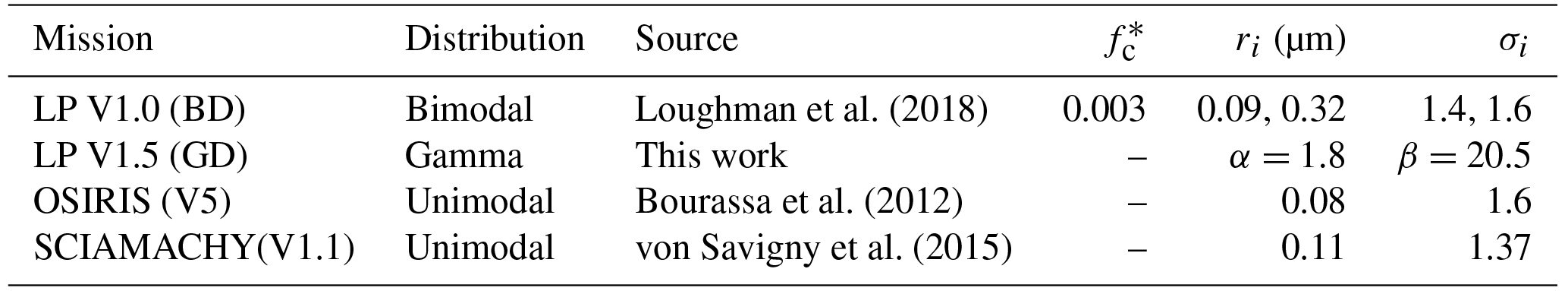
* fc is the coarse-mode fraction, which is the ratio of the number of particles of the coarse mode to the total number of particles for a bimodal lognormal distribution (Loughman et al., 2018).
Assuming that optically thin conditions prevail, the radiance sensitivity is approximately proportional to the change in aerosol extinction k at the tangent point for the LOS. The LP aerosol extinction retrieval therefore employs a nonlinear iterative technique, based on Chahine's nonlinear relaxation technique (e.g., Chahine, 1970):
where represents the state vector (i.e., extinction) at altitude zi after n iterations of the retrieval algorithm. The measurement vector represents the measured ASIm at tangent height hi=zi. The Gauss–Seidel limb scattering (GSLS) radiative transfer model (Herman et al., 1994, 1995; Loughman et al., 2004, 2015) calculates the ASIc vector at each iteration, using the extinction profile given by . The cross section and aerosol scattering phase function are calculated from an assumed ASD using Mie theory assuming spherical droplets of sulfuric acid (H2SO4). An initial guess for aerosol profile is constructed by using an aerosol extinction climatology derived from SAGE II data for the period 2000–2004. The LP algorithm performs four iterations of Eq. (3) to reach the final extinction profile. The LP aerosol product provides extinction profiles from cloud-top height to 40 km. We flag the lowest level of the retrieved aerosol profile at the cloud-top altitude, which is determined using the algorithm described in Chen et al. (2016). Potential errors due to stray light or absolute calibration bias are addressed in part through the use of altitude-normalized radiances in constructing the ASI measurement vector. Jaross et al. (2014) discuss possible remaining altitude-dependent errors from these sources.
The primary change introduced for the LP V1.5 aerosol retrieval algorithm is the revised particle size distribution described in Sect. 3. Other changes with less impact on the retrieved extinction values include the use of vector radiative transfer calculations and the implementation of intra-orbit tangent height adjustments as described by Moy et al. (2017). In addition, the V1.0 retrievals only allowed a factor-of-2 change in extinction for each iteration and executed three iterations, rather than the larger values (factor-of-5 change, four iterations) given in Loughman et al. (2018). Based on inspection of test results, we revised those parameters for the V1.5 algorithm to allow a factor-of-3 change in extinction for each iteration and four iterations of the retrieval.
Retrieval of aerosol extinction profiles from limb scattering measurements requires the specification of an aerosol size distribution (ASD) to represent the microphysical properties of the aerosol particles. Different functional forms can be selected to represent the ASD. The V1.0 LP aerosol algorithm retrieves extinction profiles by assuming a bimodal lognormal size distribution (BD):
where n(r) is the size distribution function (), i represents the ith mode of the distribution (i=1 and 2 indicate fine and coarse mode, respectively), r is the particle radius (µm), ri is the median radius, σi is the standard deviation, and Ni is the number of the particles corresponding to the mode i (cm−3). The fine- and coarse-mode size parameters of this distribution (see Table 1) are primarily based on ER-2 measurements made in August 1991, at 36∘ N, 121∘ W and 16.5 km (Pueschel et al., 1994). Since the observed coarse-mode fraction fc in the Pueschel et al. (1994) data was very high following the eruption of Mt. Pinatubo, we adjusted fc downward to provide an Ångström exponent (AE, defined in Eq. 5) of 2.0.
where k is the aerosol extinction at wavelength λ. We chose AE =2.0 as our reference because it represents the mean value of AE at 20 km altitude estimated from SAGE II (Version 7.0) aerosol extinction data (Damadeo et al., 2013) at 525 and 1020 nm taken during the period 2000–2005, when the stratosphere was relatively clean and roughly similar to the present-day stratosphere (Loughman et al., 2018).
The main motivation for using a bimodal size distribution arose from the desire to make comparisons with the existing in situ optical particle counter (OPC) data set, which generally features a bimodal size distribution at the altitudes where the stratospheric aerosol extinction is greatest (Deshler et al., 2003). However, specifying the five independent parameters (two mode radii, two mode widths and the coarse-mode fraction) needed to define this more complex distribution can be challenging. Most OPC measurements have no independent information at radii less than 0.1 µm, so that the aerosol size distribution between 0.01 and 0.1 µm is poorly defined (Kovilakam and Deshler, 2015). The lack of information in the OPC data gap region results in greater uncertainty in fitting data using the bimodal size distribution function (see Appendix A). As pointed out in Appendix A, the OPC does not count particles smaller than 0.1 µm, but the information on the smaller particles comes from super-saturating the cell so that all particles are lit up and one gets a gross count of the total number. Although a seemingly arbitrary collection of bimodal size distributions would fit the resolved OPC data equally well, the residual uncertainty results in large uncertainty in the phase function. Moreover, internal evaluation of V1.0 algorithm performance with no reference to external data sets (described in Sect. 4) and comparison of retrieved extinction profiles with SAGE III/ISS data (described in Sect. 5) also raised questions about the use of the V1.0 bimodal size distribution.
To select an alternate ASD for use in LP retrievals, we have used results from CARMA. CARMA is a sectional aerosol and cloud microphysics model that has been used to study a wide variety of problems in planetary atmospheres (Toon et al., 1979, 1988; Turco et al., 1979; Bardeen et al., 2008; Colarco et al., 2003, 2014; English et al., 2011, 2012; Yu et al., 2015). The CARMA model is coupled here to the NASA Goddard Earth Observing System (GEOS) Earth system model, a three-dimensional atmospheric general circulation model, as described in Colarco et al. (2014), and provides simulated aerosol distributions over a full range of latitude and longitude, altitude, and season. Colarco et al. (2014) describes how CARMA was implemented initially for dust and sea salt. The usage in GEOS for sulfate aerosols is a relatively new capability, with the sulfur chemistry mechanism and aerosol microphysics as in English et al. (2011) and as described and evaluated in Aquila et al. (2018). The particle size distribution is represented by 22 size bins covering a wide range of radii from 0.000267 to 2.79 µm. For this paper, we use output from simulations in which volcanic eruptions have been turned off, so that the background aerosol distribution reflects anthropogenic and nonvolcanic sources.
The aerosol optical properties can be directly calculated based on a radiative transfer model for each bin of the CARMA size distribution. However, the Mie calculation in the current LP aerosol code requires an analytic aerosol mode, rather than bin data. In this study, we use an analytical model of aerosol particle size distribution which deals with the ASD as a mean of size spectrum to accurately fit a cumulative distribution function (CDF) on the binned data using Deshler's method (Deshler et al., 2003). We have chosen the gamma distribution (GD; e.g., Chylek et al., 1992) to describe the size distribution of aerosols for OMPS/LP retrievals (Chen et al., 2018). This function is described in Eq. (6).
where n(r) is the number of particles N(r) per unit volume with a size between radius r and r+dr (), N0 is the total number density of aerosols (cm−3), α and β (µm−1) are the fitting parameters, and Γ is Euler's Gamma function. At small radii this function follows a power law, while at large radii it follows an exponential function. In contrast to the BD, which has five adjustable parameters, the gamma function has only two parameters to be specified, the shape parameter α and the scale parameter β. These parameters have a unique relationship to the effective radius:
In order to fit the GD to CARMA results, we calculate the cumulative aerosol size distribution,
where N(>r) represents the concentration of all particles larger than r. The integral is performed over a range of sizes from µm to µm. The two parameters of the GD are determined by fitting the CDF of Eq. (8) using a Levenberg–Marquardt nonlinear least squares regression algorithm. The scattering cross sections and phase functions are then calculated using Mie theory assuming spherical particles of refractive index of 1.448+0i for hydrated sulfuric acid (Palmer and Williams, 1975), which is the same as that assumed in the LP V1.0 aerosol algorithm.
We created a subset of CARMA results that is approximately consistent with the Deshler et al. (2003) long-term measurements by averaging June–July–August model results to create a climatology, then extracting aerosol size distribution values for the approximate location (41∘ N, 105∘ W) and altitude (20 km) of those measurements. We then calculated CDF fits to the CARMA results using unimodal normal distribution (UD), BD and GD functions (described in Eqs. 4 and 6) using the same fitting method. For consistency with the OPC database, CARMA bins between 0.02 and 0.1 µm were excluded from the fit. Figure 1a shows that, while these CDF fits are relatively similar, the GD function does give the best agreement with the excluded CARMA values.

Figure 1Comparison between gamma size distribution (GD), bimodal lognormal size distribution (BD) and unimodal normal distribution (UD). (a) Three cumulative size distribution fits as a function of particle radius to the normalized CARMA data at 20 km. Blue: GD; red: BD; black: UD. The black dots represent cumulative CARMA data. Data points shown as (+) were excluded from the fit. (b) Differential size distributions derived from the fitted parameters shown in (a). For comparison, the size distribution used in V1.0 (green) is also shown. Among these size distributions, the V1.0 function has the largest dN∕dlogr value at 0.1 µm and the smallest dN∕dlogr value at 0.3 µm. The phase functions derived from the V1.0 and GD are shown in Fig. 2.
Figure 1b compares the derived differential size distributions from the three fits, which are plotted as dN∕dlogr vs. r in log–log scale (here log is the logarithm to base 10). The BD function used for LP V1.0 processing is also shown for comparison. In contrast to the cumulative distribution functions shown in Fig. 1a, the differential distributions differ significantly for r≤0.1 µm. Note that the V1.0 bimodal ASD has the largest dN∕dlogr value among these distributions at r≈0.1 µm. As a result, the corresponding aerosol scattering phase function for the BD fit is closer to a Rayleigh phase function at large scattering angles (Θ>120∘), as shown in Fig. 2. Fractional differences of 40 % in this region can lead to up to a factor-of-2.5 larger extinction values at 20.5 km and at low effective reflectivities ρ (see Sect. 4), where the derived extinctions are roughly inversely proportional to the P(Θ), as discussed by Loughman et al. (2018). Conflating Figs. 1b, 2, A1b and A2, it is concluded that the Mie phase function depends strongly on the peak in dN∕dlogr. A larger dN∕dlogr value at around 0.1 µm (i.e., narrower distribution width) causes larger P(Θ) value at large scattering angles.
Limb scattering measurements from other satellite instruments have also been used to retrieve stratospheric aerosol extinction profiles, with their own choices of particle size distribution. Bourassa et al. (2012) used a unimodal size distribution based on Deshler et al. (2003) OPC data to retrieve aerosol extinction from OSIRIS radiance data at 750 nm. Rieger et al. (2014) not only used the same function and initial parameters but also investigated the addition of 1530 nm radiance data to enable the simultaneous retrieval of extinction and mode radius. Rieger et al. (2018) evaluated the errors associated with both unimodal and bimodal size distributions in the OSIRIS and SCIAMACHY retrieval algorithms. Von Savigny et al. (2015) used a unimodal size distribution based on different OPC data (Deshler, 2008) to retrieve aerosol extinction from SCIAMACHY radiance data at 750 nm, although the radiance data were not normalized with 470 nm radiance data. Malinina et al. (2018) used an alternate approach with SCIAMACHY data in which radiances at seven wavelengths between 750 and 1530 nm were included and the number density profile was held constant. This allowed the simultaneous retrieval of mode radius and distribution width for cloud-free observations at tropical latitudes (20∘ S to 20∘ N). We include the parameters for the OSIRIS and SCIAMACHY size distributions in Table 1 and show the corresponding phase functions in Fig. 2. While we did not create test data sets using those size distributions, we note that their differences from the V1.0 phase function in Fig. 2 are in the same direction as the gamma distribution (i.e., lower value at backscattered angles) but smaller in magnitude. So we would expect that processing LP data with one of these unimodal size distributions would yield less change relative to our V1.0 product than the gamma distribution adopted for V1.5. The improved agreement with SAGE III data for V1.5 extinction data shown in Figs. 10–13 suggests that we would not want to adopt a size distribution that produces less change in extinction.
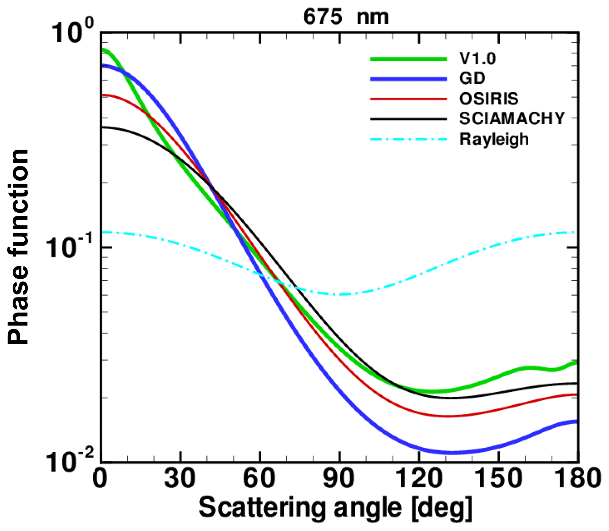
Figure 2Phase functions at the 675 nm wavelength derived from the aerosol size distributions listed in Table 1, including OMPS V1.0 (green), GD (blue), OSIRIS (red) and SCIAMACHY (black). The Rayleigh phase function is also shown as a dashed line for reference. The V1.0 P(Θ) is closer to Rayleigh behavior at large scattering angles despite having more coarse particles (r>0.5 µm) than others. This is because phase function at 675 nm is sensitive to particle radii at 0.1 µm.
We have selected the gamma size distribution derived from CARMA results in this work to assess the impact of ASD on stratospheric aerosol extinction profile retrieval from OMPS/LP limb measurements. The two fitted parameters (α=1.8 and β=20.5) determined from the GD fit at 20 km produce an AE of 2.0 and a reff of 0.18 µm. These values match the average values determined from SAGE II Version 7.0 data (Thomason et al., 2008; Damadeo et al., 2013) during the 2000–2005 period. Hereafter, this resultant ASD derived from the CARMA results will be labeled as V1.5 ASD, while the ASD assumed in LP V1 will be labeled as V1.0 ASD. The current LP retrieval algorithm assumes that the size distribution is height independent, so that one function is used to represent the aerosol size distribution at all heights. We plan to use CARMA model results in a future version of the algorithm to incorporate variation in ASD and P(Θ) with altitude, latitude, season and after a volcanic eruption. While we find in this study a general improvement in the quality of the OMPS LP aerosol retrievals by adopting the physically based and self-consistent CARMA-produced particle size distribution, we acknowledge here that the use of this particular model is not intended as a definitive prescription for the OMPS LP algorithms. The model is of course subject to a variety of uncertainties in its own right, in terms of formulation and implementation of its physical algorithms, and generally speaking the modeling of the stratospheric aerosol particle size distribution and composition is nontrivial and a subject of ongoing work by a number of researchers. For example, the version of the model used here does not yet include the possible impacts of volcanic eruptions on the background particle distribution, nor does it include the impacts of nonsulfate aerosols that may be important in the UTLS (e.g., organics). We recognize that to push the approach taken here further, for example, to use a model-based climatology of aerosol properties to define altitude- and location-specific properties to be used in the OMPS LP algorithms, requires at a minimum a more complete implementation of the relevant physics in the model (i.e., addition of missing species) and a thorough and independent evaluation of its capabilities and quality. Determining the particle size distribution based on model results is a challenging task. The assumptions inherent in any complex model can sometimes require arbitrary choices that influence the calculated results. So the size distribution adopted here for LP V1.5 aerosol extinction retrievals may not yield equally good results in all situations.
Figure 3a shows the impact on the gamma distribution P(Θ) of changing the mode parameters by ±10 % relative to the baseline mode, for the range of scattering angles viewed during a single OMPS/LP orbit (Chen et al., 2018). It is apparent that the phase function is quite sensitive to β. A ±10 % change in β can produce a ±10 % change in the calculated aerosol phase function at moderate scattering angles (Θ= 70–100∘), whereas a ±10 % change in α only yields a ±3 % change in phase function at . Examination of the corresponding differential distribution curves (not shown) indicates that increasing α produces an increase in the peak dN∕dlogr value, whereas increasing β shifts this peak to larger values of r. The changes in P(Θ) (Fig. 3a) lead to corresponding significant changes in retrieved aerosol extinctions, as shown in Fig. 3b. The changes in aerosol extinction are approximately anti-correlated with the phase function variations, although smaller in magnitude. The small-scale structures of the extinction data are caused by the variation in scene reflectivity along the orbit, which is discussed further in Sect. 4.
It is important to point out that OMPS/LP measurements cover a wide range of scattering angles with a well-defined latitude dependence. Figure 4 shows the variation of Θ with latitude for two dates corresponding to solstice conditions. Note that high values of Θ are always observed in the Southern Hemisphere (SH), while low values of Θ are observed in the Northern Hemisphere (NH). The impact of this sampling on measured ASI is discussed in Sect. 4.
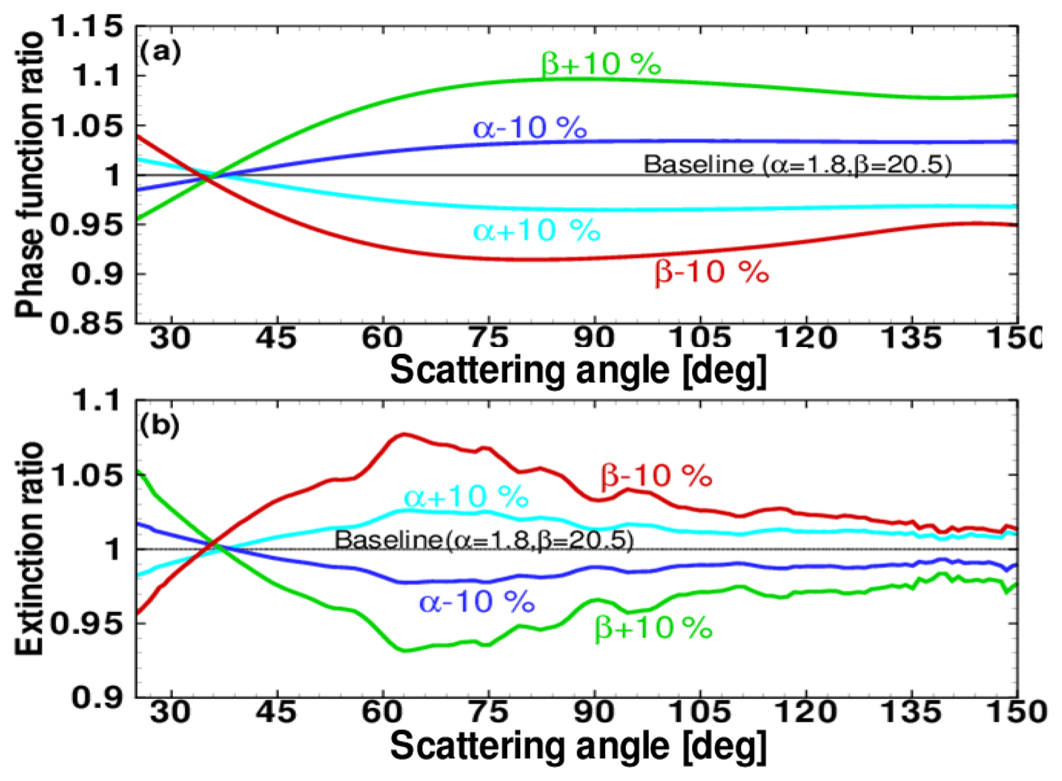
Figure 3This figure shows how simulated phase function and retrieved extinction change when α and β are perturbed by ±10 % of the baseline values (α=1.8 and β=20.5). All the phase functions and the extinctions shown are divided by the baseline data (black lines). (a) Ratio of the perturbed phase function to the baseline phase function. (b) Ratio of the perturbed extinction to the baseline extinction. The extinctions are retrieved using the simulated phase function and OMPS/LP measurements at 20.5 km for a single orbit on 12 September 2016. Note that the two curves are roughly anti-correlated, but the fractional change in extinction is about half of the change in P(Θ) depending on the single scattering angle Θ. (From Chen et al., 2018.)
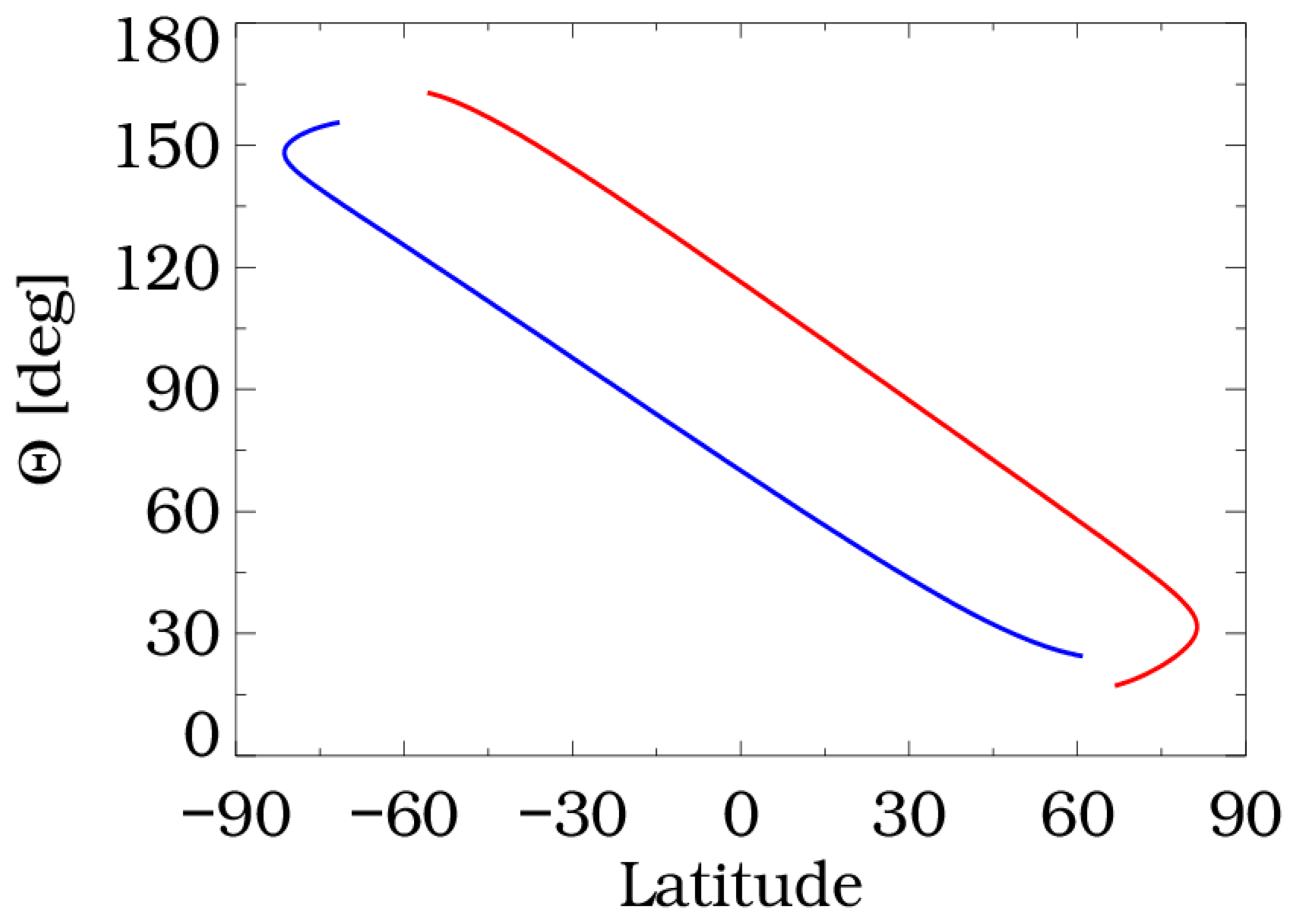
Figure 4Variation of scattering angle (Θ) vs. latitude for OMPS/LP measurements on 22 June (red) and 22 December (blue). (From Loughman et al., 2018.)
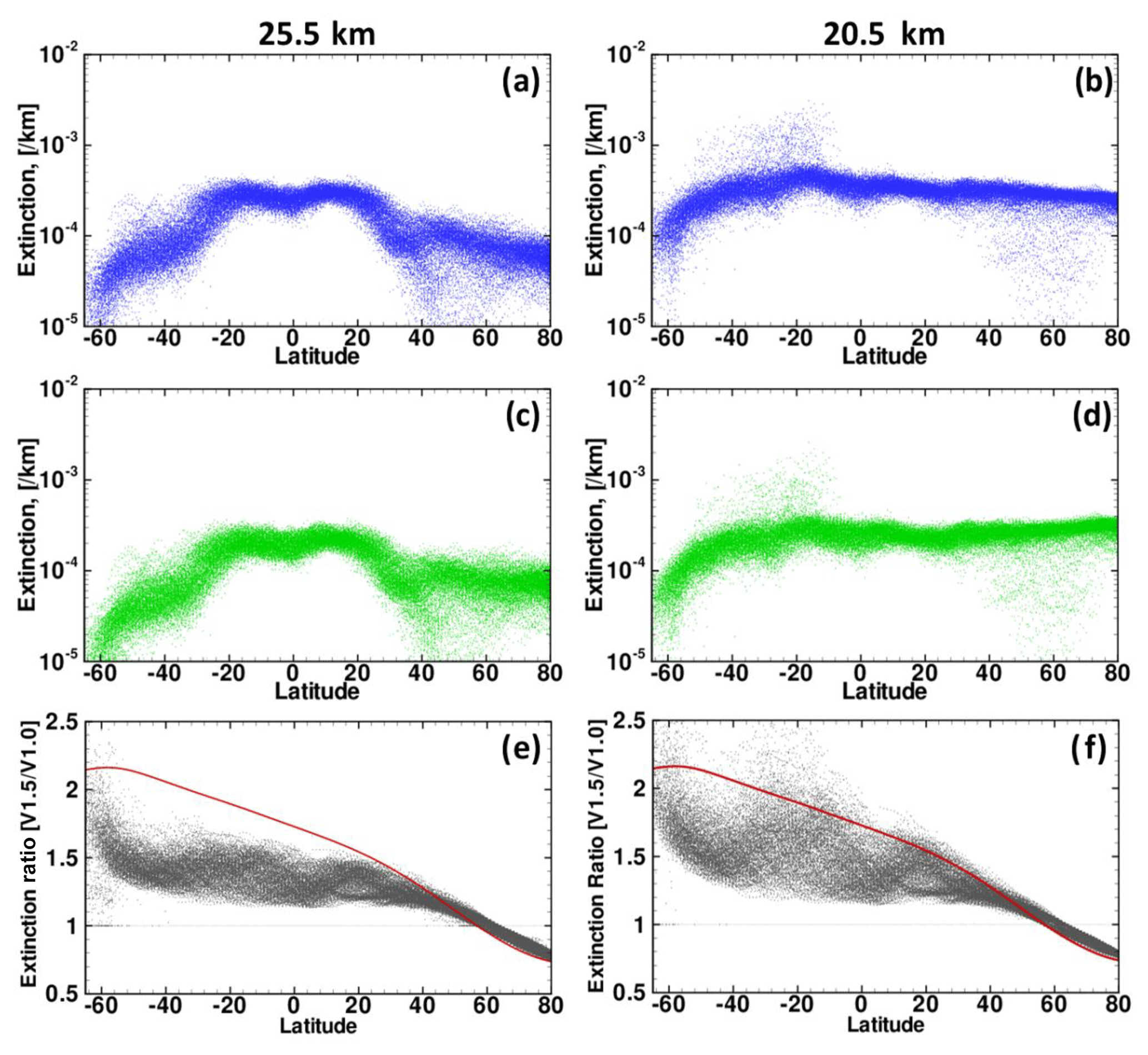
Figure 5Scatter diagrams of retrieved aerosol extinctions for the V1.5 ASD (blue) and the V1.0 ASD (green) at 25.5 km (a, c, e) and 20.5 km (b, d, f) for an entire month during the Calbuco period 21 April ∼ 20 May 2015. The black dots in the bottom panel show extinction ratios (V1.5 ∕ V1.0), and the red lines show the inverse of the P(Θ) ratio (PV1.0Θ ∕ PV1.5Θ). The ratio of extinctions has large variability at a given latitude, though the P(Θ) ratios do not. (From Chen et al., 2018.)
In Sect. 3, we described the creation of the gamma aerosol size distribution model derived from CARMA results. To understand the quality of the present aerosol size distribution and to estimate the uncertainty associated with the retrieved aerosol extinction, we first perform the aerosol retrieval code runs for conditions without a significant volcanic eruption. This provides a baseline situation. To evaluate the performance of the presented aerosol size distribution, aerosol extinction profiles were retrieved from OMPS/LP measurements before and after the Calbuco volcano eruption to see if the volcanic eruption can be captured by the new model. This eruption occurred in Chile (41.3∘ S, 72.6∘ W) on 22 April 2015 and had a clear impact on the stratospheric aerosol distribution.
Figure 5 shows scatter diagrams of retrieved aerosol extinctions at 20.5 and 25.5 km as a function of latitude for the V1.5 ASD (blue) and from V1.0 ASD (green), as well as their ratios (kV1.5 ∕ kV1.0, black) for the entire month of data following the Calbuco eruption (Chen et al., 2018). Extinction values from the V1.5 retrievals (top row) have a similar latitude dependence to the V1.0 retrieval values (middle row) for both 25.5 and 20.5 km. However, the extinction ratio (kV1.5 ∕ kV1.0) decreases in magnitude from high Southern Hemisphere latitudes to high Northern Hemisphere latitudes. The inverse of the phase function ratio, i.e., , is also shown for comparison in the bottom row of Fig. 5. The observed change in extinction from the V1.0 ASD to the V1.5 ASD is typically smaller than the corresponding phase function change at all SH latitudes and at NH latitudes less than ∼40∘ N. This difference is caused in part by the “smearing” effect of multiple scattering, which becomes more pronounced at lower altitudes (note the larger scatter of extinction ratio values in Fig. 5f). The change in extinction ratio is greater than 1.0 at most latitudes due to the change in phase function presented in Fig. 2 and the mapping between LP scattering angle and measurement latitude illustrated in Fig. 4.
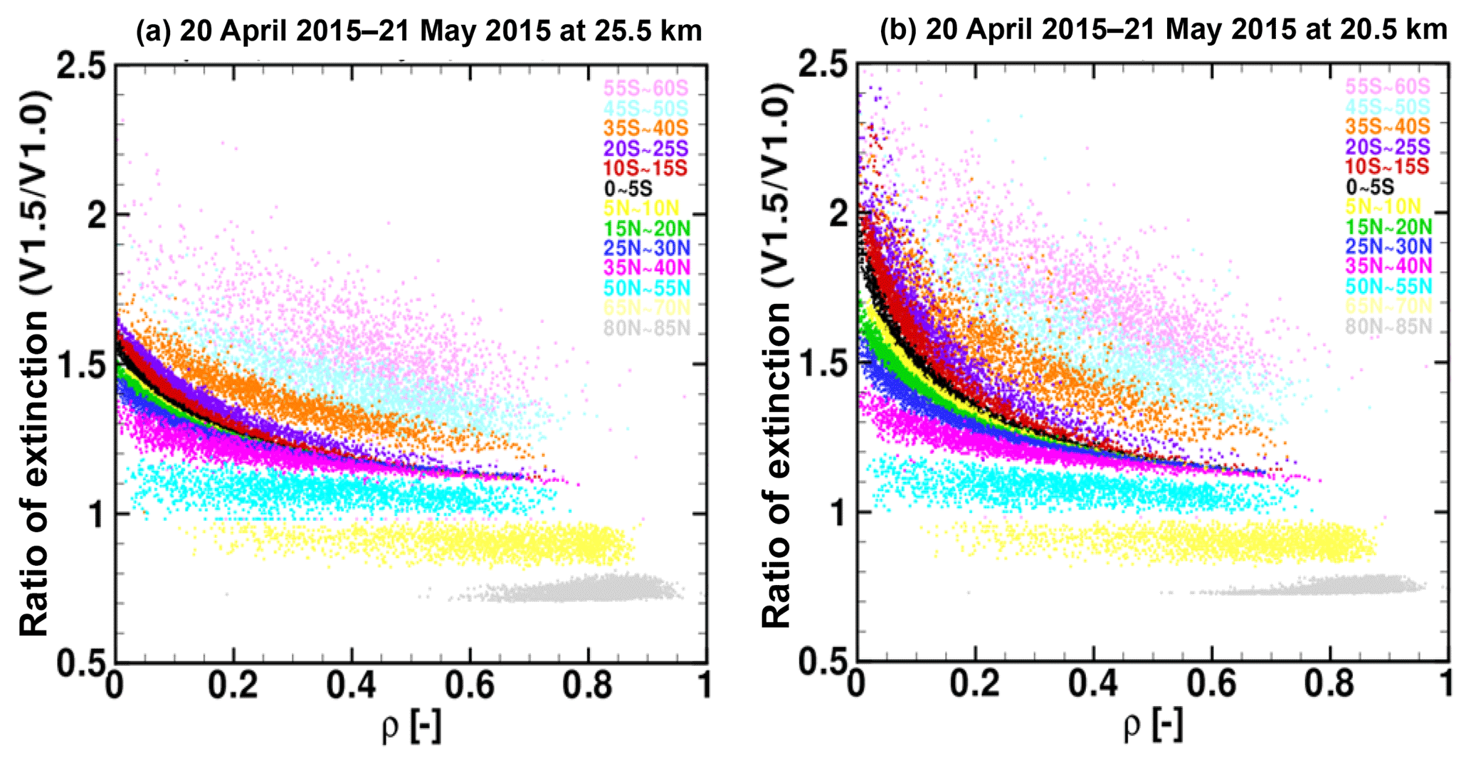
Figure 6Scatterplots of extinction ratio (V1.5 ∕ V1.0) as a function of effective reflectivity (ρ) for different latitude bins at 25.5 km (a) and 20.5 km (b). The figure shows that the extinction ratios vary nonlinearly with the effective reflectivity, especially for reflectivity <0.2. The shape of the function changes considerably with latitude and altitude. (From Chen et al., 2018.)

Figure 7Zonal mean of ASI residuals (ASIm–ASIc) at 20.5 km as a function of latitude for wavelengths at 352, 430, 508, 600, 745 and 869 nm for one entire year in 2017. The V1.5 ASD (blue) does a better job in explaining the measured ASI relationship than the V1.0 ASD (green).
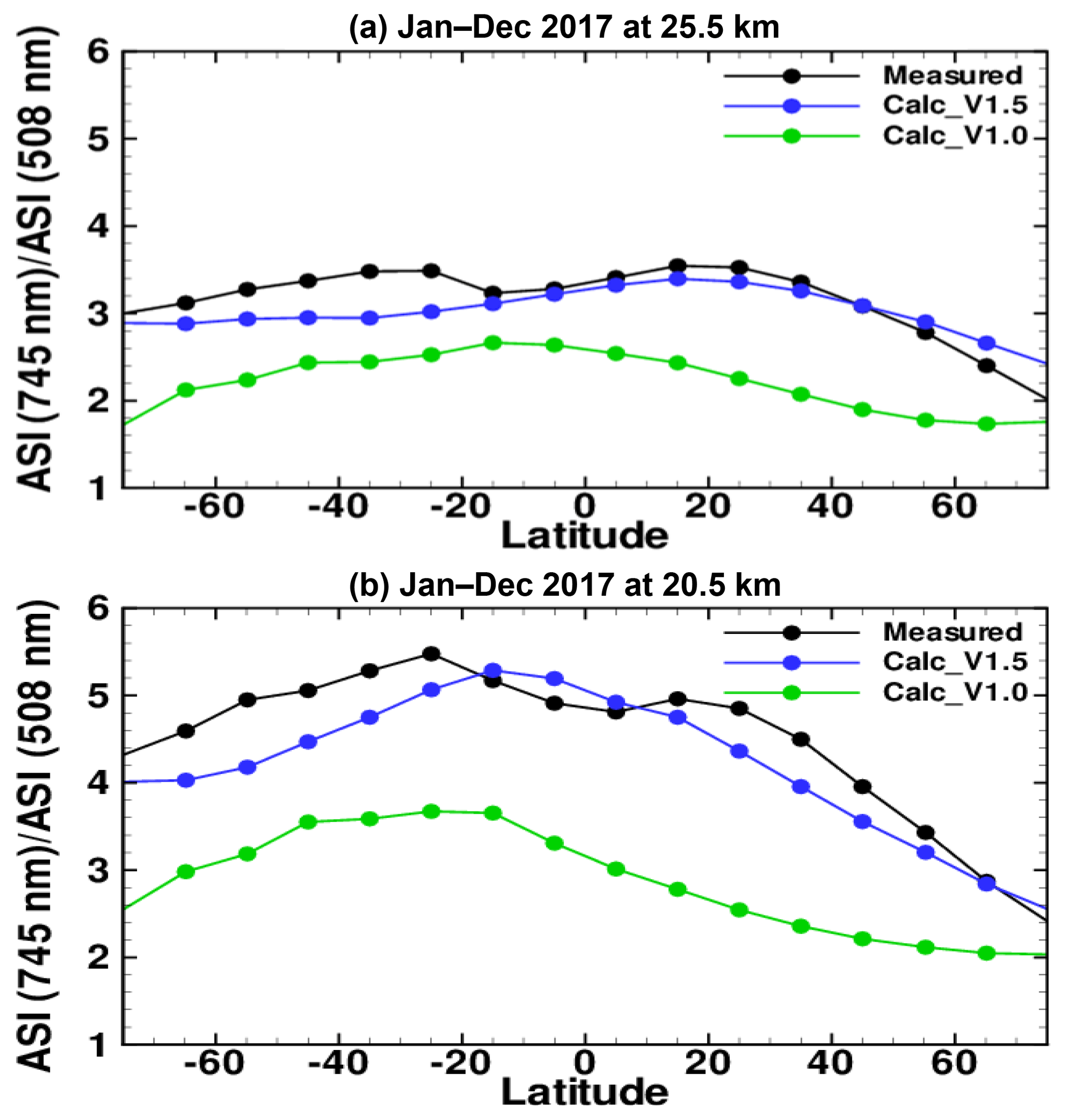
Figure 8Zonal mean of ratio ASI(745 nm) ∕ ASI(508 nm) at 25.5 km (a) and 20.5 km (b) as a function of latitude. Calculated values using the V1.5 ASD (blue dots) are more effective in explaining the measured ASI ratios (black dots) than the V1.0 ASD (green dots).
Figure 5e and f show significantly more variability in extinction ratio of kV1.5 ∕ kV1.0 at SH latitudes, which is correlated mainly with the variation of effective reflectivity ρ. ρ is derived from the LP measurements at 675 nm to represent Earth surface reflectance. In the LP retrieval algorithm, ρ is determined by comparing the measured data to model radiances at 40 km using a Lambertian surface (Loughman et al., 2018). This “Lambert-equivalent” reflectivity (LER) value typically differs from the true surface reflectivity due to diffuse upwelling radiation (DUR) contributions from clouds, aerosols and other features within the scene. As discussed in Loughman et al. (2018), the effect of Rayleigh scattering and aerosol scattering on radiances is not strictly additive. The relationship between the large variability in extinction ratio shown in Fig. 5 and variations in LER is further illustrated in Fig. 6. The dependence of the extinction ratio (kV1.5 ∕ kV1.0) on ρ can become nonlinear at low reflectivity (ρ<0.2), and the slope of the linear portion of this figure (ρ>0.2) varies with latitude. The nonlinear variation in extinction ratio at ρ<0.2 clearly increases in magnitude when moving from 25.5 to 20.5 km, showing the altitude dependence of the additional contribution from Rayleigh scattering.
While the altitude normalization used to construct the ASI measurement vector in Eq. (1) reduces the effect of DUR in the LP aerosol extinction profile retrieval considerably, there are second-order effects present that make ASI sensitive to ρ at altitudes where there are aerosols. This occurs because DUR is scattered by the aerosols at an average scattering angle close to 90∘, while the direct solar radiation is scattered at a wider range of angles shown in Fig. 4. For singly scattered (SS) radiances, assuming that the attenuation of SS radiance along the LOS is small, ASI is proportional to the product of k and P(Θ). So in this approximation the spectral dependence of ASI should be determined by the spectral dependence of k⋅P(Θ), which is determined by ASD. Hence, if the assumed ASD is correct, the measured and calculated spectral dependence of ASI should be consistent.
In Fig. 7, ASI residuals (difference between the measured ASI and the calculated ASI) from V1.0 and V1.5 retrievals at 20.5 km are plotted as a function of latitude for wavelengths not used in the LP aerosol retrieval (352, 430, 508, 600, 745, 869 nm) for the V1.5 test processing of the 1-year data set. Residuals at the retrieval wavelength (675 nm) are not shown because they are very close to zero for both cases. The residuals produced by the V1.5 ASD are closer to zero than the V1.0 residuals for all wavelengths, indicating that the gamma function ASD more effectively represents the OMPS/LP measurements.
Figure 8 shows the ratio of ASI(745 nm) ∕ ASI(508 nm) at 20.5 and 25.5 km as a function of latitude, using LP measurements and the calculated ASI values from the V1.0 and V1.5 ASDs. The agreement between measured and calculated ASI ratio is significantly better for the V1.5 ASD, demonstrating the improved representation of spectral dependence with this function. Similar figures can be constructed for other combinations of LP wavelengths. The 1-year results shown in Figs. 7 and 8 demonstrate how internal analysis of LP aerosol retrieval results can help identify the most appropriate ASD to use for these retrievals. We note that the ability to distinguish between ASDs is better in the NH, where LP scattering angles are lower and the relative uncertainty in P(Θ) is reduced. We therefore use comparisons with external measurements to obtain additional validation of our choice for the V1.5 ASD.

Figure 9SAGE III/ISS solar occultation coverage compared to OMPS/LP coverage. Red: sunrises; black: sunsets; light blue: OMPS/LP.

Figure 10Time series of individual extinctions at 20.5 km observed by LP V1.5 (blue), V1.0 (green), SAGE sunrises (red) and SAGE sunsets (black) for six different latitude bins centered at 45∘ S, 25∘ S, 5∘ S, 5∘ N, 25∘ N and 45∘ N during the comparison period. The pink and yellow lines show the median of aerosol extinctions at 20.5 km from LP V1.5 and V1.0, respectively.
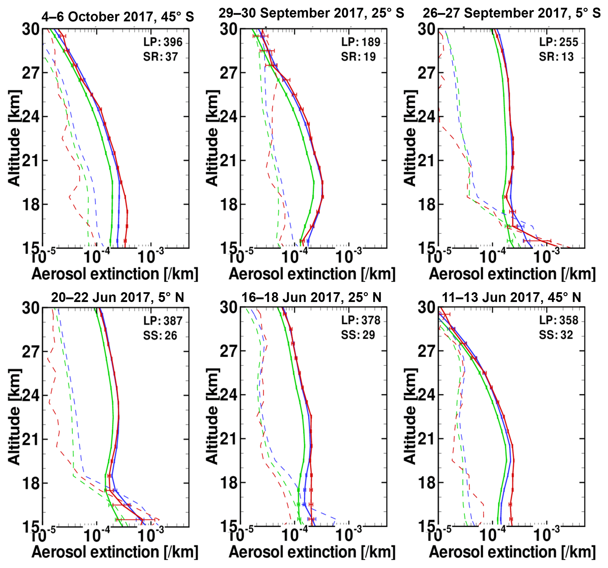
Figure 11Comparison of zonal mean profiles of collocated SAGE III/ISS (red solid lines), LP Version 1 (green solid lines) and LP Version 1.5 (blue solid lines) aerosol extinction profiles for six different latitude bins centered at 45∘ S, 25∘ S, 5∘ S, 5∘ N, 25∘ N and 45∘ N. The dashed lines show the corresponding standard deviations. The horizontal error bars indicate standard error of the mean, . The numbers at the top shows the number of measurements averaged for each profile.
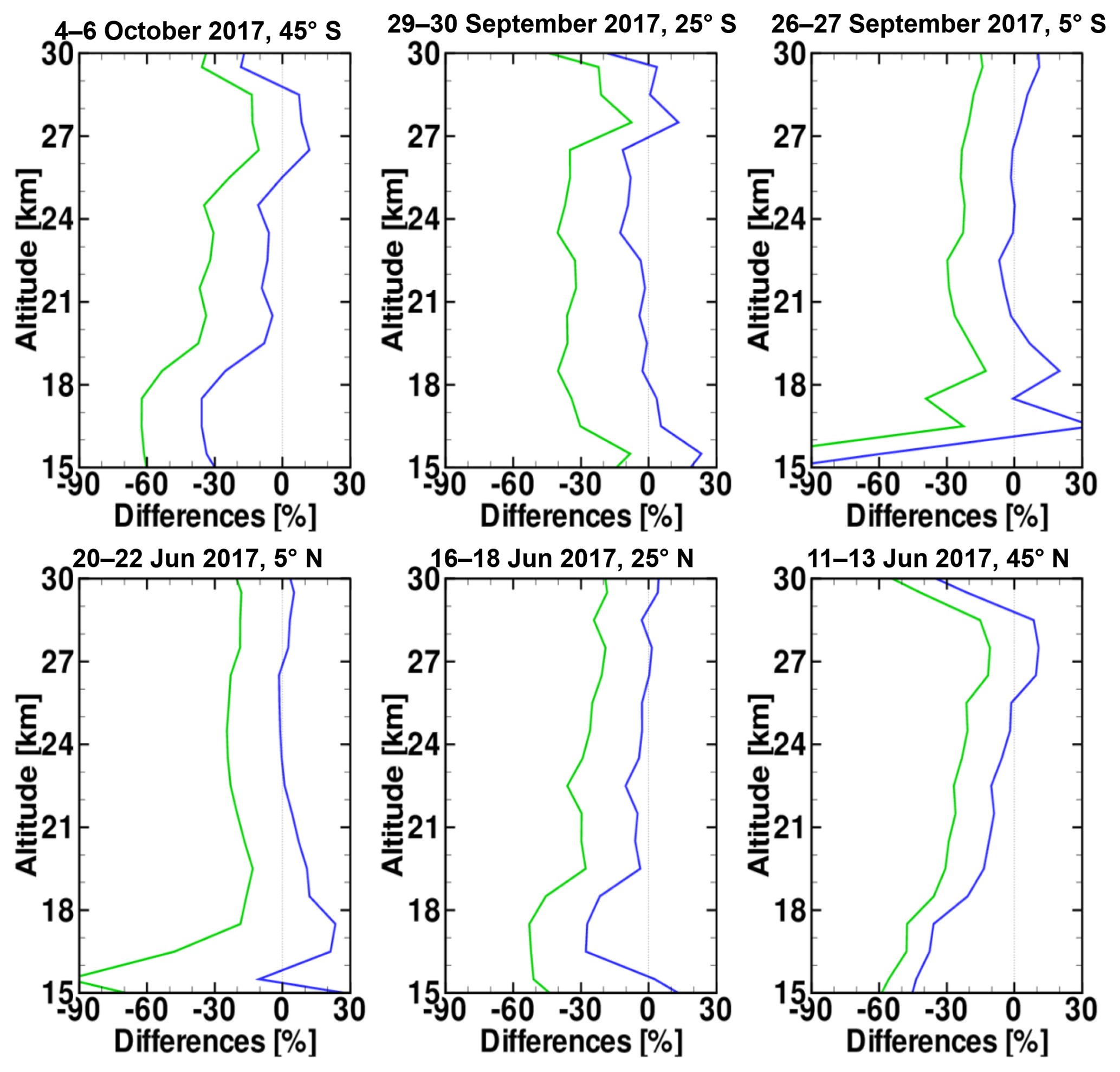
Figure 12Relative differences of the mean aerosol extinction profiles between 675 nm OMPS/LP and 676 nm SAGE III/ISS. Difference . Blue lines: LP V1.5–SAGE; green lines: LP V1.0–SAGE.
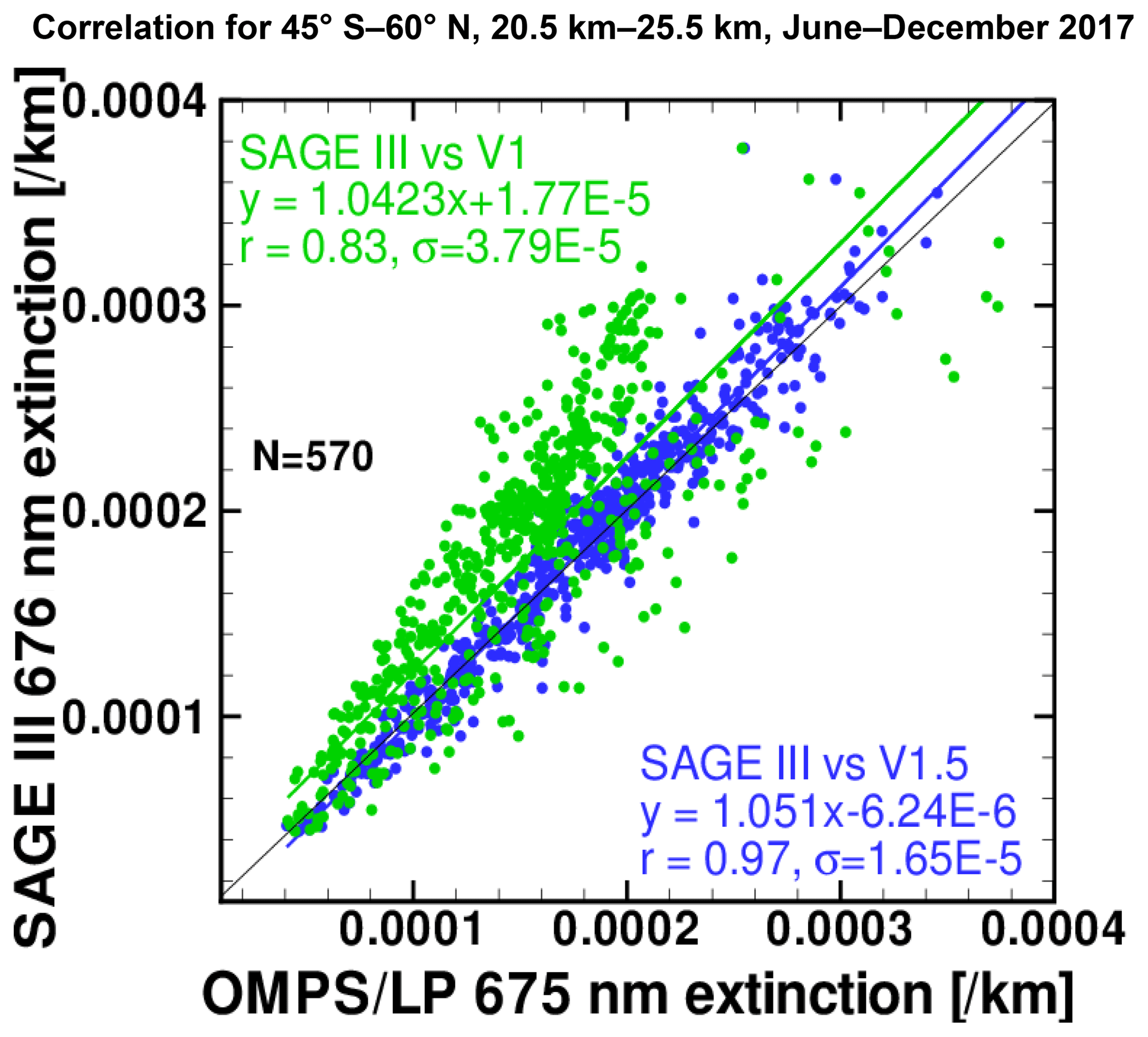
Figure 13Correlation plot of SAGE III/ISS vs. OMPS/LP V1.5 (blue) and SAGE III/ISS vs. OMPS/LP V1.0 (green) zonal mean aerosol extinctions in 10∘ latitude bins from 45∘ S to 60∘ N between 20 and 25 km for the entire comparison period. The blue and green lines show the linear regressions between the data points, and the thin black line represents a 1 : 1 relationship. The correlation coefficient r, the standard deviation of the differences (x−y) σ and the number of elements N used to compute r are also shown.
The Stratospheric Aerosol and Gas Experiment on the International Space Station (SAGE III/ISS) developed by NASA Langley Research Center (LaRC) was launched to the International Space Station in February 2017. SAGE III/ISS provides limb occultation measurements of aerosols and gases in the stratosphere and upper troposphere (Chu and Veiga, 1998). The SAGE series of occultation measurements have been extensively evaluated and compared with other space-based instruments and have been found to have relatively high precision and accuracy (Bourassa et al., 2012). A general description of the solar occultation measurement technique is provided by McCormick et al. (1979). The ISS travels in a low Earth orbit at an altitude of 330–435 km at an inclination of 51.6∘. With these orbital parameters, solar occultation measurement opportunities cover a large range of latitudes (between 60∘ S and 60∘ N). The solar occultation measurement Version 5 Level 2 data were collected during the period June–December 2017. SAGE III/ISS scientists have released this initial data set (which includes retrievals of ozone, aerosols and nitrogen dioxide from solar occultation measurements) in order to solicit feedback from the international atmospheric science community. Figure 9 shows the spatiotemporal coverage of the available data sets used for this study. Profiles of aerosol extinction at nine wavelengths reported by SAGE III/ISS (384.2, 448.5, 520.5, 601.6, 676.0, 756.0, 869.2, 1021.2, 1544.0 nm) are provided from the surface or cloud top to an altitude of 45 km, with a vertical resolution of 0.5 km at the tangent point location. We have compared OMPS/LP aerosol extinction retrievals at 675 nm and SAGE III/ISS aerosol extinction retrievals at 676 nm directly, using SAGE III samples that correspond to the OMPS/LP 1 km altitude grid. For OMPS/LP, only data from the center slit were taken into consideration, and all data below the cloud height were rejected.
Figure 10 shows time series of OMPS/LP and SAGE III/ISS extinctions for six 10∘ latitude bins at 20.5 km from June to December 2017. Red and black dots show individual measurements from sunrise (SR) and sunset (SS), blue and green dots represent LP V1.5 and V1.0, and pink and yellow lines are the median of the individual LP extinctions, respectively. SAGE III/ISS data are available for groups of a few days at each latitude, while OMPS/LP measurements provide daily global coverage. This time series demonstrates that reasonable agreement is observed between LP V1.5 data (pink line) and SAGE III/ISS data (red and black clusters), while LP V1.0 retrievals typically show lower extinction values except in the Northern Hemisphere during winter. This difference is consistent with the scattering angle dependence discussed in Sect. 4, since LP measures at small scattering angles at this time. Pattern differences between LP V1.5 and V1.0 reflect the impact of aerosol size distribution on aerosol extinction. Large variability throughout most of the time series can be explained by differences in spatial or temporal sampling. The enhanced extinctions at 20.5 km observed by both LP and SAGE III in September–December in the Northern Hemisphere are likely associated with the enormous pyrocumulus events caused by the British Columbia wildfires in August 2017.
Further indication of the level of agreement between OMPS/LP and SAGE III/ISS is provided by comparing the zonal average profiles. For this comparison, a relatively broad collocation requirement of ±5∘ latitude was used, and longitudinal differences were ignored in order to maintain a minimal comparison set size. The variation in SAGE III sampling illustrated in Fig. 9 limits each zonal average to 2–3 consecutive days of measurements. The data have been binned and averaged to the OMPS/LP reporting altitudes for direct comparison.
Figure 11 shows the zonal mean extinction profiles between 15 and 30 km altitude in 6±5∘ latitude bins. For each latitude bin, the mean OMPS/LP profile is usually composed of between 180 and 400 measurements, while the number of SAGE III profiles used in each average is much smaller, typically between 20 and 40 profiles. For all latitude bins, the general agreement between LP V1.5 and SAGE III is quite good except at lower altitudes (<18 km), where larger differences may indicate limitations in the LP retrieval algorithm. In contrast, LP V1.0 retrievals are systematically lower than SAGE III over the entire profile. This improvement in agreement gives us confidence that the revised ASD used in the V1.5 processing is more appropriate for describing OMPS/LP measurements.
Figure 12 shows relative differences between the mean LP and SAGE profiles using the same latitude bins shown in Fig. 11. The absolute value of the relative differences between LP V1.5 and SAGE III is generally <10 % for 19–29 km, demonstrating good agreement. The relative differences are larger below 18 km, likely due to uncertainties in LP aerosol retrievals at these altitudes.
Figure 13 shows a scatterplot of individual zonal mean extinction values from each data set between 20.5 and 25.5 km, selected for collocation within 10∘ latitude between 45∘ S and 60∘ N for the entire comparison period. Linear regression fits between OMPS/LP and SAGE III extinction data show a clear improvement in correlation coefficient from SAGE III vs. V1.0 to SAGE III vs. V1.5 (r=0.83 to r=0.97), with a concurrent reduction in standard deviation of the differences σ (defined as ) for the V1.5 fit by a factor of 2. These results give further quantitative evidence that the gamma function ASD is appropriate for OMPS/LP aerosol extinction retrievals. Because of the large variation of phase function with scattering angle (Fig. 2) and the strong dependence between scattering angle and latitude for OMPS LP (Fig. 4), the size distribution determined here is not necessarily the optimum choice for a satellite instrument with a different measurement geometry resulting from a different orbit.
This paper describes the derivation of a revised aerosol size distribution function to retrieve aerosol extinction profiles from OMPS/LP limb scattering radiance measurements. We use results from the CARMA microphysical model as a basis for the revised ASD to take advantage of CARMA's large range of particle size information. We find that using an ASD based on a gamma function fit (designated V1.5) requires fewer free parameters than our previous choice of a bimodal lognormal ASD (designated V1.0) and is more consistent with the CARMA particle size results. Evaluation of LP observed radiances is complicated by the measurement geometry (typically backward scattering in the SH, forward scattering in the NH) and the corresponding variation in phase function, as well as variations in scene reflectivity. The V1.5 ASD improves the performance of radiance-based retrieval algorithm internal validation tests, including reducing the magnitude of residuals between calculated and measured radiance and spectral dependence.
We also evaluated our revised ASD by comparing V1.5 retrieved extinction profiles to SAGE III measurements during June–December 2017. Relative differences between collocated zonal mean profiles are less than 10 % between 19 and 29 km, with increased differences below 18 km. Regression fits to all data between 20 and 25 km show a better correlation coefficient between SAGE III data and LP retrievals with the V1.5 ASD (r=0.97) and a factor-of-2 improvement in standard deviation of the differences compared to results using the previous V1.0 ASD. We anticipate using the extensive CARMA model results in the future to determine additional ASDs for LP retrievals that can better represent natural aerosol variability in latitude, altitude and season. CARMA results can also be used to develop a more effective ASD for aerosol retrievals following a volcanic eruption.
The OMPS LP Version 1.5 aerosol data product will be available through the NASA Goddard Earth Sciences Data and Information Services Center (GES DISC) at https://disc.gsfc.nasa.gov. The DOI for this product (Deland, 2016) is https://doi.org/10.5067/2CB3QR9SMA3F. The SAGE III/ISS Version 5 Level 2 data are available at https://doi.org/10.5067/ISS/SAGEIII/SOLAR_BINARY_L2-V5.0 for the binary version and at https://doi.org/10.5067/ISS/SAGEIII/SOLAR_HDF4_L2-V5.0 for the HDF version, NASA ASDC (2018).
One of the longest and most comprehensive records of local stratospheric aerosol conditions comes from the University of Wyoming's optical particle counters (OPCs) carried on weather balloons at Laramie, Wyoming, USA (41∘ N), at altitudes up to 30 km. The instrument measures the number of aerosol particles in several size bins, ranging from 0.15 to 2 µm radius. In most cases, a bimodal lognormal size distribution (BD) is used to fit OPC data if there are enough different particle sizes measured. For background stratospheric conditions, however, OPC data may not provide sufficient information about smaller particles (r<0.15 µm) to determine a robust BD fit.
An example of this situation is illustrated in Fig. A1, which shows four bimodal lognormal distribution fits to the same OPC data at 20 km altitude, all having similar Ångström exponents of approximately 2.4, but each with a different values of coarse-mode fraction fc. The fitted parameters as well as the calculated AE and reff are given in Table A1. This topic is discussed further by Nyaku et al. (2018).
All four fits to the OPC data are equally good, but they differ from each other significantly in the radius range between 0.01 and 0.1 µm because the gap in OPC size bins limits the ability to constrain a fit. As a consequence, the differences between the ASDs near 0.1 µm lead to significant changes in P(Θ) for backward scattering conditions, as shown in Fig. A2. It can be seen that P(Θ) is quite sensitive to the value of dN∕dlogr around r=0.1 µm when . ASD_1 (black) and ASD_2 (red) have larger values of dN∕dlogr around r=0.1 µm, shown in Fig. A1. Larger values of P(Θ) derived from the two ASDs in this range are therefore closer to a Rayleigh scattering behavior.
Table A1Four BD fits to OPC data measured at Laramie, Wyoming, on 12 April 2010 at 20 km.

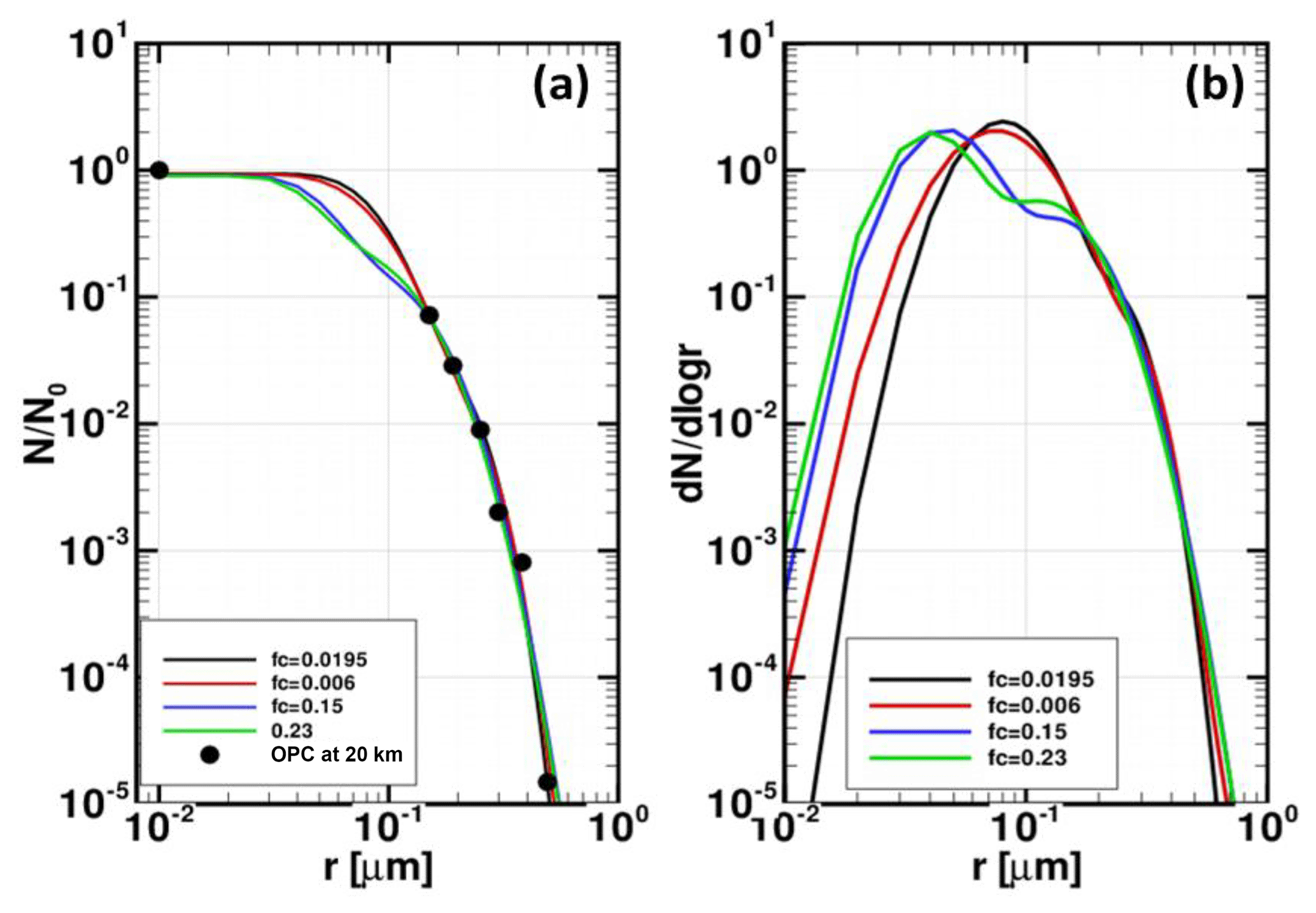
Figure A1Estimated bimodal lognormal cumulative distributions (a) and differential distributions (b) for nonvolcanic OPC measurement on 12 April 2000 at 20 km (Kovilakam and Deshler, 2015). Measurements are shown as black dots on the left panel. Each fit with a different coarse-mode fraction, fc, which is the ratio of the number of particles of the coarse mode to the total number of particles for a bimodal lognormal distribution.
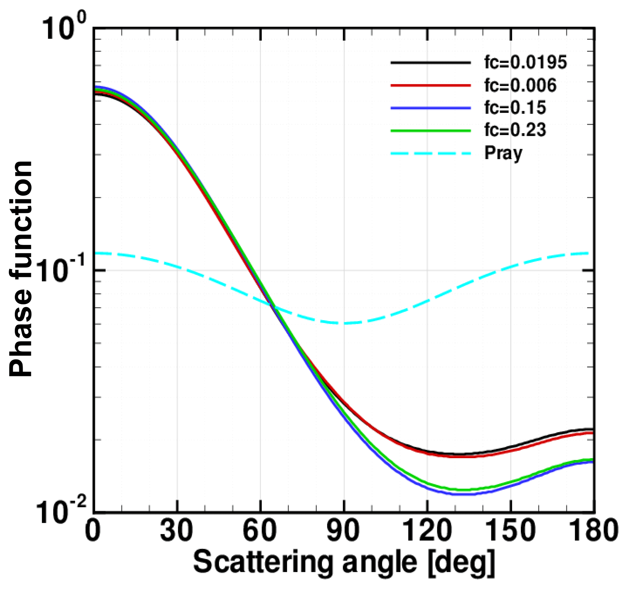
Figure A2Aerosol phase functions at 675 nm as a function of single scattering angle for the four ASDs listed in Table A1.
The authors declare that they have no conflict of interest.
We thank the OMPS/LP team at NASA Goddard and Science Systems and
Applications, Inc. (SSAI) for help in producing the data used in this study.
We also would like to thank Tong Zhu for her technical support. Zhong Chen
and Matthew DeLand were supported by NASA contract NNG17HP01C.
Edited by: Piet Stammes
Reviewed by: three anonymous referees
Aquila, V., Colarco, P. R., Bian, H., Chin, M., Darmenov, A., Oman, L., Rollins, A., Taha, G., and Tan, Q.: Simulating stratospheric aerosol with the NASA Goddard Earth System Model Chemistry Climate Model (GEOSCCM), Geosci. Model Dev., in preparation, 2018.
Bardeen, C. G., Toon, O. B., Jensen, E. J., Marsh, D. R., and Harvey, V. L.: Numerical simulations of the three-dimensional distribution of meteoric dust in the mesosphere and upper stratosphere, J. Geophys. Res., 113, D17202, https://doi.org/10.1029/2007jd009515, 2008.
Bertaux, J. L., Kyrölä, E., Fussen, D., Hauchecorne, A., Dalaudier, F., Sofieva, V., Tamminen, J., Vanhellemont, F., Fanton d'Andon, O., Barrot, G., Mangin, A., Blanot, L., Lebrun, J. C., Pérot, K., Fehr, T., Saavedra, L., Leppelmeier, G. W., and Fraisse, R.: Global ozone monitoring by occultation of stars: an overview of GOMOS measurements on ENVISAT, Atmos. Chem. Phys., 10, 12091–12148, https://doi.org/10.5194/acp-10-12091-2010, 2010.
Bourassa, A., Degenstein, D., and Llewellyn, E.: Retrieval of stratospheric Bourassa, A. E., Degenstein, D. A., and Llewellyn, E. J.: Retrieval of stratospheric aerosol size information from OSIRIS limb scattered sunlight spectra, Atmos. Chem. Phys., 8, 6375–6380, https://doi.org/10.5194/acp-8-6375-2008, 2008.
Bourassa, A. E., Rieger, L. A., Lloyd, N. D., and Degenstein, D. A.: Odin-OSIRIS stratospheric aerosol data product and SAGE III intercomparison, Atmos. Chem. Phys., 12, 605–614, https://doi.org/10.5194/acp-12-605-2012, 2012.
Chahine, M.: Inverse problems in radiative transfer: A determination of atmospheric parameters, J. Atmos. Sci., 27, 960–967, 1970.
Chen, Z., DeLand, M., and Bhartia, P. K.: A new algorithm for detecting cloud height using OMPS/LP measurements, Atmos. Meas. Tech., 9, 1239–1246, https://doi.org/10.5194/amt-9-1239-2016, 2016.
Chen, Z., Bhartia, P. K., Loughman, R., and Colarco, P.: Impact of aerosol size distribution on extinction and spectral dependence of radiances measured by the OMPS Limb profiler instrument, Atmos. Meas. Tech. Discuss., https://doi.org/10.5194/amt-2018-4, in review, 2018.
Chu, W. and Veiga, R.: SAGE III/EOS, Proc. SPIE, 3501, 52–60, https://doi.org/10.1117/12.577943, 1998.
Chu, W., McCormick, M., Lenoble, J., Brogniez, C., and Pruvost, P.: SAGE II inversion algorithm, J. Geophys. Res., 94, 8339–8351, 1989.
Chylek, P., Damiano, P., and Shettle, E. P.: Infrared emittance of water clouds, J. Atmos. Sci., 49, 1459–1472, 1992.
Colarco, P., Toon, O., and Holben, B.: Saharan dust transport to the Caribbean during PRIDE: 1. Influence of dust sources and removal mechanisms on the timing and magnitude of downwind aerosol optical depth events from simulations of in situ and remote sensing observations, J. Geophys. Res., 108, 8589, https://doi.org/10.1029/2002JD002658, 2003.
Colarco, P. R., Nowottnick, E. P., Randles, C. A., Yi, B., Yang, P., Kim, K.-M., Smith, J. A., and Bardeen, C. G.: Impact of radiatively interactive dust aerosols in the NASA GEOS-5 climate model: Sensitivity to dust particle shape and refractive index, J. Geophys. Res.-Atmos., 119, 753–786, https://doi.org/10.1002/2013JD020046, 2014.
Damadeo, R. P., Zawodny, J. M., Thomason, L. W., and Iyer, N.: SAGE version 7.0 algorithm: application to SAGE II, Atmos. Meas. Tech., 6, 3539–3561, https://doi.org/10.5194/amt-6-3539-2013, 2013.
Deland, M.: OMPS-NPP L2 LP Aerosol Extinction Vertical Profile swath daily 3slit V1, Greenbelt, MD, USA, Goddard Earth Sciences Data and Information Services Center (GES DISC), Accessed: [27 November 2018], https://doi.org/10.5067/2CB3QR9SMA3F, 2016.
Deshler, T.: A review of global stratospheric aerosol: Measurement, importance, life cycle, and local stratospheric aerosol, Atmos. Res., 90, 223–232, https://doi.org/10.1016/j.atmosres.2008.03.016, 2008.
Deshler, T., Hervig, M. E., Hofmann, D. J., Rosen, J. M., and Liley, J. B.: Thirty years of in situ stratospheric aerosol size distribution measurements from Laramie, Wyoming (41∘ N) using balloon-borne instruments, J. Geophys. Res., 108, 4167, https://doi.org/10.1029/2002JD002514, 2003.
English, J. M., Toon, O. B., Mills, M. J., and Yu, F.: Microphysical simulations of new particle formation in the upper troposphere and lower stratosphere, Atmos. Chem. Phys., 11, 9303–9322, https://doi.org/10.5194/acp-11-9303-2011, 2011.
English, J. M., Toon, O. B., and Mills, M. J.: Microphysical simulations of sulfur burdens from stratospheric sulfur geoengineering, Atmos. Chem. Phys., 12, 4775–4793, https://doi.org/10.5194/acp-12-4775-2012, 2012.
Flynn, L. E., Seftor, C. J., Larsen, J. C., and Xu, P.: The Ozone Mapping and Profiler Suite, in: Earth Science Satellite Remote Sensing, edited by: Qu, J. J., Gao, W., Kafatos, M., Murphy, R. E., and Salomonson, V. V., Springer, Berlin, 279–296, https://doi.org/10.1007/978-3-540-37293-6, 2007.
GES DISC: NASA Goddard Earth Sciences Data and Information Services Center, available at: https://disc.gsfc.nasa.gov, last access: 22 November 2018.
Herman, B. M., Ben-David, A., and Thome, K. J.: Numerical techniques for solving the radiative transfer equation for a spherical shell atmosphere, Appl. Optics, 33, 1760–1770, 1994.
Herman, B. M., Caudill, T. R., Flittner, D. E., Thome, K. J., and Ben David, A.: Comparison of the Gauss-Seidel spherical polarized radiative transfer code with other radiative transfer codes, Appl. Optics, 34, 4563–4572, 1995.
Jaross, G., Bhartia, P. K., Chen, G., Kowitt, M., Haken, M., Chen, Z., Xu, P., Warner, J., and Kelly, T.: OMPS Limb Profiler instrument performance assessment, J. Geophys. Res.-Atmos., 119, 4399–4412, https://doi.org/10.1002/2013JD020482, 2014.
Kovilakam, M. and Deshler, T.: On the accuracy of stratospheric aerosol extinction derived from in situ size distribution measurements and surface area density derived from remote SAGE II and HALOE extinction measurements, J. Geophys. Res.-Atmos., 120, 8426–8447, https://doi.org/10.1002/2015JD023303, 2015.
Kramarova, N. A., Bhartia, P. K., Jaross, G., Moy, L., Xu, P., Chen, Z., DeLand, M., Froidevaux, L., Livesey, N., Degenstein, D., Bourassa, A., Walker, K. A., and Sheese, P.: Validation of ozone profile retrievals derived from the OMPS LP version 2.5 algorithm against correlative satellite measurements, Atmos. Meas. Tech., 11, 2837–2861, https://doi.org/10.5194/amt-11-2837-2018, 2018.
Loughman, R., Flittner, D., Nyaku, E., and Bhartia, P. K.: Gauss–Seidel limb scattering (GSLS) radiative transfer model development in support of the Ozone Mapping and Profiler Suite (OMPS) limb profiler mission, Atmos. Chem. Phys., 15, 3007–3020, https://doi.org/10.5194/acp-15-3007-2015, 2015.
Loughman, R., Bhartia, P. K., Chen, Z., Xu, P., Nyaku, E., and Taha, G.: The Ozone Mapping and Profiler Suite (OMPS) Limb Profiler (LP) Version 1 aerosol extinction retrieval algorithm: theoretical basis, Atmos. Meas. Tech., 11, 2633–2651, https://doi.org/10.5194/amt-11-2633-2018, 2018.
Loughman, R. P., Griffioen, E., Oikarinen, L., Postylyakov, O. V., Rozanov, A., Flittner, D. E., and Rault, D. F.: Comparison of radiative transfer models for limb viewing scattered sunlight measurements, J. Geophys. Res., 109, D06303, https://doi.org/10.1029/2003JD003854, 2004.
Malinina, E., Rozanov, A., Rozanov, V., Liebing, P., Bovensmann, H., and Burrows, J. P.: Aerosol particle size distribution in the stratosphere retrieved from SCIAMACHY limb measurements, Atmos. Meas. Tech., 11, 2085–2100, https://doi.org/10.5194/amt-11-2085-2018, 2018.
McCormick, M. P., Hamill, P., Pepin, T. J., Chu, W. P., Swissler, T. J., and McMaster, L. R.: Satellite studies of the stratospheric aerosol, B. Am. Meteorol. Soc., 60, 1038–1047, 1979.
Moy, L., Bhartia, P. K., Jaross, G., Loughman, R., Kramarova, N., Chen, Z., Taha, G., Chen, G., and Xu, P.: Altitude registration of limb-scattered radiation, Atmos. Meas. Tech., 10, 167–178, https://doi.org/10.5194/amt-10-167-2017, 2017.
NASA ASDC: Atmospheric Science Data Center, available at: http://eosweb.larc.nasa.gov, last access: 22 November 2018.
Nyaku, E., Loughman, R., Bhartia, P. K., Deshler, T., Chen, Z., and Colarco, P.: The sensitivity of the stratospheric aerosol phase function to aerosol size distribution models, Atmos. Meas. Tech., in preparation, 2018.
Palmer, K. F. and Williams, D.,: Optical constants of sulfuric acid; Application to the clouds of Venus, Appl. Optics, 14, 208–219, 1975.
Pueschel, R., Russell, P., Allen, D., Ferry, G., Snetsinger, K., Livingston, J., and Verma, S.: Physical and optical properties of the Pinatubo volcanic aerosol: Aircraft observations with impactors and a Sun-tracking photometer, J. Geophys. Res., 99, 12915–12922, https://doi.org/10.1029/94JD00621, 1994.
Rault, D. F. and Loughman, R. P.: The OMPS Limb Profiler Environmental Data Record algorithm theoretical basis document and expected performance, IEEE T. Geosci. Remote, 51, 2505–2527, 2013.
Ridley, D. A., Solomon, S., Barnes, J. E., Burlakov, V. D., Deshler, T., Dolgii, S. I., Herber, A. B., Nagai, T., Neely III, R. R., Nevzorov, A. V., Ritter, C., Sakai, T., Santer, B. D., Sato, M., Schmidt, A., Uchino, O., and Vernier, J. P.: Total volcanic stratospheric aerosol optical depths and implications for global climate change, Geophys. Res. Lett., 41, 7763–7769, https://doi.org/10.1002/2014GL061541, 2014.
Rieger, L. A., Bourassa, A. E., and Degenstein, D. A.: Stratospheric aerosol particle size information in Odin-OSIRIS limb scatter spectra, Atmos. Meas. Tech., 7, 507–522, https://doi.org/10.5194/amt-7-507-2014, 2014.
Rieger, L. A., Malinina, E. P., Rozanov, A. V., Burrows, J. P., Bourassa, A. E., and Degenstein, D. A.: A study of the approaches used to retrieve aerosol extinction, as applied to limb observations made by OSIRIS and SCIAMACHY, Atmos. Meas. Tech., 11, 3433–3445, https://doi.org/10.5194/amt-11-3433-2018, 2018.
Thomason, L. W., Burton, S. P., Luo, B.-P., and Peter, T.: SAGE II measurements of stratospheric aerosol properties at non-volcanic levels, Atmos. Chem. Phys., 8, 983–995, https://doi.org/10.5194/acp-8-983-2008, 2008.
Thomason, L. W., Moore, J. R., Pitts, M. C., Zawodny, J. M., and Chiou, E. W.: An evaluation of the SAGE III version 4 aerosol extinction coefficient and water vapor data products, Atmos. Chem. Phys., 10, 2159–2173, https://doi.org/10.5194/acp-10-2159-2010, 2010.
Toon, O. B., Turco, R., Hamill, P., Kiang, C., and Whitten, R.: A one-dimensional model describing aerosol formation and evolution in the stratosphere: II. Sensitivity studies and comparison with observations, J. Atmos. Sci., 36, 718–736, 1979.
Toon, O. B., Turco, R. P., Westphal, D., Malone, R., and Liu, M. S.: A multidimensional model for aerosols – description of computational analogs, J. Atmos. Sci., 45, 2123–2143, 1988.
Turco, R., Hamill, P., Toon, O., Whitten, R., and Kiang, C.: A one-dimensional model describing aerosol formation and evolution in the stratosphere: I. Physical processes and mathematical analogs, J. Atmos. Sci., 36, 699–717, 1979.
von Savigny, C., Ernst, F., Rozanov, A., Hommel, R., Eichmann, K.-U., Rozanov, V., Burrows, J. P., and Thomason, L. W.: Improved stratospheric aerosol extinction profiles from SCIAMACHY: validation and sample results, Atmos. Meas. Tech., 8, 5223–5235, https://doi.org/10.5194/amt-8-5223-2015, 2015.
Winker, D. M., Vaughan, M. A., Omar, A. H., Hu, Y., Powell, K. A., Liu, Z., Hunt, W. H., and Young, S. A.: Overview of the CALIPSO mission and CALIOP data processing algorithms, J. Atmos. Ocean. Tech., 26, 2310–2323, https://doi.org/10.1175/2009JTECHA1281.1, 2009.
Yu, P., Toon, O. B., Neely, R. R., Martinsson, B. G., and Brenninkmeijer, C. A. M.: Composition and physical properties of the Asian Tropopause Aerosol Layer and the North American Tropospheric Aerosol Layer, Geophys. Res. Lett., 42, 2540–2546, https://doi.org/10.1002/2015GL063181, 2015.