Joint retrieval of surface reflectance and aerosol properties with continuous variation of the state variables in the solution space – Part 1: theoretical concept

This paper presents a new algorithm for the joint retrieval of surface reflectance and aerosol properties with continuous variations of the state variables in the solution space. This algorithm, named CISAR (Combined Inversion of Surface and AeRosol), relies on a simple atmospheric vertical structure composed of two layers and an underlying surface. Surface anisotropic reflectance effects are taken into account and radiatively coupled with atmospheric scattering. For this purpose, a fast radiative transfer model has been explicitly developed, which includes acceleration techniques to solve the radiative transfer equation and to calculate the Jacobians. The inversion is performed within an optimal estimation framework including prior information on the state variable magnitude and regularisation constraints on their spectral and temporal variability. In each processed wavelength, the algorithm retrieves the parameters of the surface reflectance model, the aerosol total column optical thickness and single-scattering properties. The CISAR algorithm functioning is illustrated with a series of simple experiments.

1 Introduction

Radiative coupling between atmospheric scattering and surface reflectance processes prevents the use of linear relationships for the retrieval of aerosol properties over land surfaces. The discrimination between the contribution of the signal reflected by the surface and that scattered by aerosols represents one of the major issues when retrieving aerosol properties using space-borne passive optical observations over land surfaces. Conceptually, this problem can be modelled to solve a radiative system composed of at least two sets of layers, where the upper layers include aerosols and the bottom ones represent the soil–vegetation strata. The problem can be further complicated by the intrinsic anisotropic radiative behaviour of natural surfaces due to the mutual shadowing of the scattering elements, which is also affected by the amount of incident radiation (Govaerts et al., 2016, 2010b). In most cases, an increase in aerosol concentration is responsible for an increase in the fraction of diffuse sky radiation which, in turn, smooths the effects of surface reflectance anisotropy. Though multispectral information is critical for the retrieval of aerosol properties, the spectral dimension alone does not allow full characterisation of the underlying surface reflectance, which often offers a significant contribution to the total signal observed at the satellite level. In this regard, the additional information contained in multispectral and multi-angular observations has proven essential to characterising aerosol properties over land surfaces.

Pinty et al. (2000a) pioneered the development of a retrieval method dedicated to the joint retrieval of surface reflectance and aerosol properties based on the inversion of a physically based radiative model. This method has been subsequently improved to permit the processing of any geostationary satellites accounting for their actual radiometric performance (Govaerts and Lattanzio, 2007). This new versatile version of Pinty's algorithm has permitted the generation of a global surface albedo product from archived data acquired by operational geostationary satellites around the globe (Govaerts et al., 2008). These data included observations acquired by an old generation of radiometers with only one broad solar channel on board the European Meteosat First Generation satellite, the US Geosynchronous Operational Environmental Satellite (GOES) and the Japanese Geostationary Meteorological Satellite (GMS). It is now routinely applied in the framework of the Sustained and COordinated Processing of Environmental satellite data for Climate Monitoring (SCOPE-CM) initiative for the generation of essential climate variables (Lattanzio et al., 2013). An improved version of this algorithm has been proposed by Govaerts et al. (2010b) to take advantage of the multispectral capabilities of Meteosat Second Generation Spinning Enhanced Visible and Infrared Imager (MSG SEVIRI) operated by EUMETSAT and includes an optimal estimation (OE) inversion scheme using a minimisation approach based on the Marquardt–Levenberg method (Marquardt, 1963).

The strengths and weaknesses of the algorithm proposed by Govaerts et al. (2010b) are discussed in Sect. 2. In their approach, the solutions of the radiative transfer equation (RTE) are pre-calculated and stored in look-up tables (LUTs) for a limited number of state variable values. Aerosol properties are limited to six different models dominated either by fine or coarse particles. Two major drawbacks result from the use of predefined aerosol models stored in precomputed LUTs. Firstly, only a limited region of the solution space is sampled as a result of the reduced range of variability for state variables stored in the LUTs. For instance, in order to reduce the size of the LUTs, Pinty et al. (2000b) limit the maximum aerosol optical thickness to 1. Secondly, the use of predefined aerosol models constitutes a major drawback since the solution space is not continuously sampled.

Dubovik et al. (2011) and Diner et al. (2012), among others, demonstrated the advantages of a retrieval approach based on continuous variations of the aerosol properties as opposed to a LUT-based approach relying on a set of predefined aerosol models. Even considering a large number of aerosol models, LUT-based approaches underperform compared to methods with multivariate continuity in the solution space (Kokhanovsky et al., 2010).

A new joint surface reflectance–aerosol properties retrieval approach is presented here that overcomes the limitations resulting from precomputed RTE solutions stored in LUTs.

The advantages of a continuous variation of the aerosol properties in the solution space against a LUT-based approach is discussed in Sect. 3. The proposed method expresses the single-scattering albedo and phase function values as a linear mixture of basic aerosol models. The forward radiative transfer model that includes the Jacobians, i.e. the partial derivative, is described in Sect. 4. With the exception of gaseous transmittance, this model no longer relies on LUTs, and the RTE is explicitly solved. The inversion method is described in Sect. 5. Finally, the ability to express aerosol single-scattering properties as a linear combination is in illustrated Sect. 6 with simulated data representing various scenarios, including small and large particles. Practical aspects of the application of the CISAR algorithm for the retrieval of both surface and aerosol properties from actual satellite data are addressed in Luffarelli and Govaerts (2018) (hereafter referred to as Part 2).

2 Lessons learned from previous approaches

Pinty et al. (2000a) proposed an algorithm for the joint retrieval of surface reflectance and aerosol properties to demonstrate the possibility of generating essential climate variables (ECVs) from data acquired by operational weather geostationary satellites. Due to limited operational computational resources available at that time in the EUMETSAT ground segment, where the data were processed, the development of this algorithm was subject to strong constraints. The RTE solutions were precomputed and stored in LUTs with a very coarse resolution, limiting the maximum aerosol optical thickness (AOT) to 1, which represented a severe limitation over the Sahara region where AOT values can easily exceed such a limit. Furthermore, the radiative coupling between aerosol scattering and gaseous absorption was not taken into account. This algorithm, referred to as geostationary surface albedo (GSA), has been subsequently modified by Govaerts and Lattanzio (2007) to include an estimation of the retrieval uncertainty. This updated version has permitted the generation of a global aerosol product derived from observations acquired by operational weather geostationary satellites (Govaerts et al., 2008). Since then, it has been routinely applied in the framework of the SCOPE-CM initiative to generate a climate data record (CDR) of surface albedo (Lattanzio et al., 2013).

The GSA algorithm has been further improved for the processing of SEVIRI data on board MSG for the retrieval of the total column AOT from observations acquired in three solar bands centred at 0.6, 0.8 and 1.6 µm (Govaerts et al., 2010b; Wagner et al., 2010). The method developed by these authors relies on an OE approach wherein surface reflectance and daily aerosol load are simultaneously retrieved. The inversion is performed independently for each aerosol model and the one with the smallest cost function is selected. A physically based radiative transfer model accounting for non-Lambertian surface reflectance and its radiative coupling with atmospheric scattering is inverted against daily accumulated SEVIRI observations. However, this land daily aerosol (LDA) algorithm suffers from two major limitations: (i) the use of predefined aerosol models, and (ii) the algorithm delivers only one mean aerosol value per day when applied to MSG SEVIRI data (Govaerts et al., 2010a). This latter issue has been addressed by Luffarelli et al. (2016), who retrieve an aerosol optical thickness value for each SEVIRI observation. The former issue prevents a continuous variation of the state variables characterising the aerosol single-scattering properties as required to find the minimum of the cost function. A consistent implementation of such an approach is not straightforward since aerosol models are defined as prior knowledge of the observed medium but uncertainties cannot be easily assigned to this decision. Consequently, the estimated retrieval uncertainty is inconsistent as it does not account for the use of prior information and its associated uncertainties.

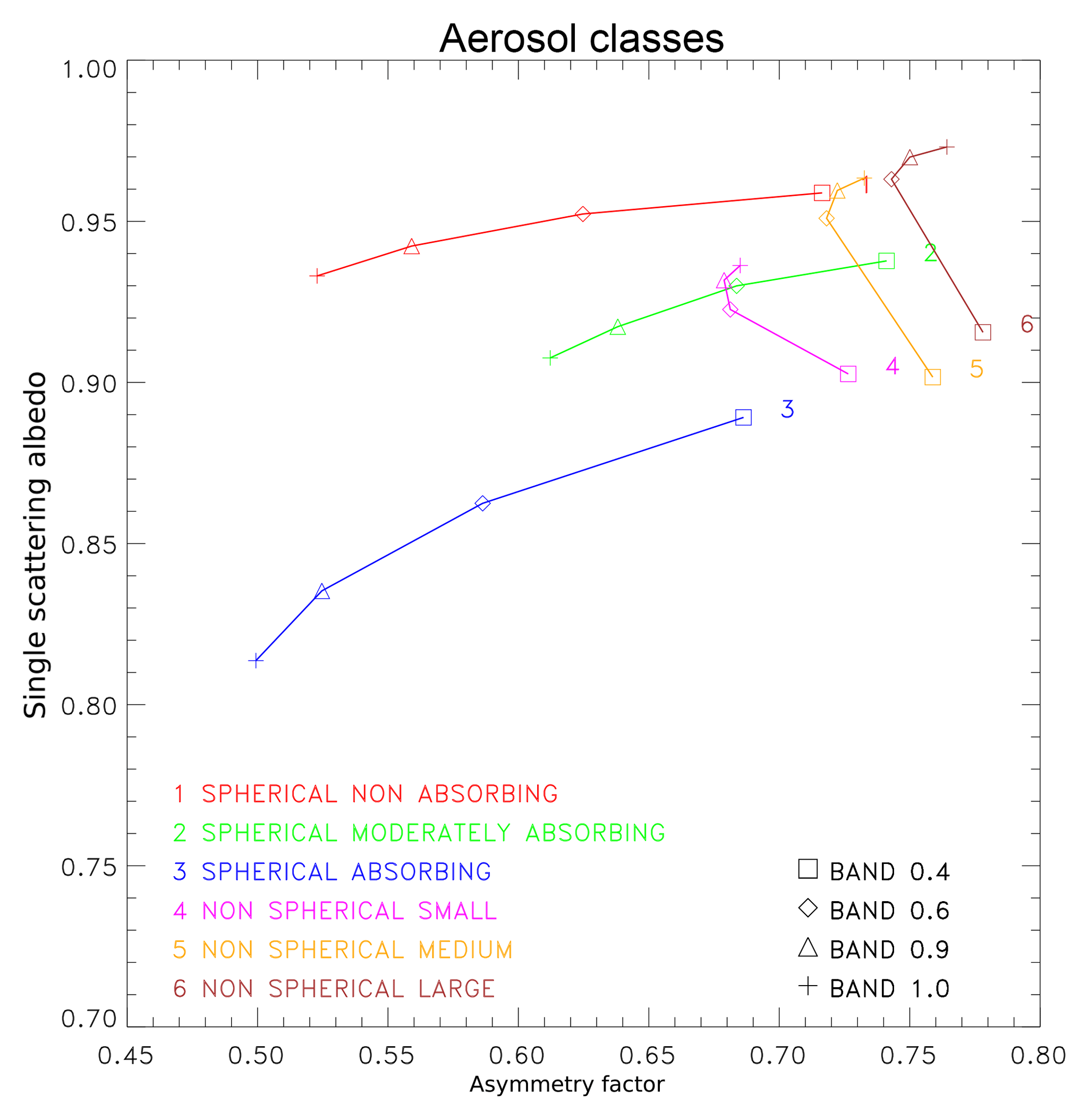
Figure 1 Aerosol dual-mode models based on Govaerts et al. (2010b) in the {g,ω₀} space derived from the aggregation of aerosol single-scattering properties retrieved from AERONET observations (Dubovik et al., 2006). Classes 1 to 3 are dominated by the fine mode and 4 to 6 by the coarse one.

Diner et al. (2012) demonstrated the advantages of a retrieval method based on continuous variations of aerosol single-scattering properties in the solution space as opposed to a LUT-based approach derived for a limited number of predefined aerosol models. Dubovik et al. (2011) proposed an original method for the retrieval of aerosol microphysical properties, which also does not necessitate the use of predefined aerosol models. This method retrieved more than 100 state variables, therefore requiring a considerable number of observations, such as those provided by multi-angular and -polarisation radiometers like Polarisation et Anisotropie des Réflectances Au SOmmet de l'Atmosphère (PARASOL) (Serene and Corcoral, 2006) or the future Multi-viewing Multi-channel Multi-polarization Imaging (3MI) instrument on board EUMETSAT's Polar System Second Generation (Manolis et al., 2013). Instruments delivering such a large number of observations are rather scarce, as most of the current passive optical sensors do not offer instantaneous multi-angular observation capabilities nor information on polarization. The primary objective of this paper is to address the limitations resulting from conventional approaches based on LUTs and/or a limited number of predefined aerosol models by proposing a method that can be applied to observations acquired by single or multi-view instruments.

3 Continuous variation of aerosol properties in the solution space

Aerosol single-scattering properties include the single-scattering albedo ω₀ and the phase function Φ in RTE. Govaerts et al. (2010b) explained the benefits of representing predefined aerosol models in a two-dimensional solution space composed of these aerosol single-scattering properties. For the sake of clarity, they limited the phase function in that 2-D space to the first term of the Legendre coefficients, i.e. the asymmetry parameter g. However, one should keep in mind that the reasoning applied in this section should be applied to the entire phase function Φ. These aerosol single-scattering properties are themselves determined by aerosol microphysical properties, such as the particle size distribution, shape and their complex index of refraction. The objective of retrievals that assume aerosol models is to provide a reasonable sampling of the {g,ω₀} space. Omitting areas of that space may produce biased retrievals, as discussed in Govaerts et al. (2010b). The inversion process proposed by in this paper relies on a set of six models which have been defined from AErosol RObotic NETwork (AERONET) data aggregation (Dubovik et al., 2006). That choice of models was intended to provide a sampling of solution space representative of real-world conditions. The inversion is repeated for each aerosol class and the result with the best fit is reported, rather than having continuously varying aerosol properties, as would be preferable.

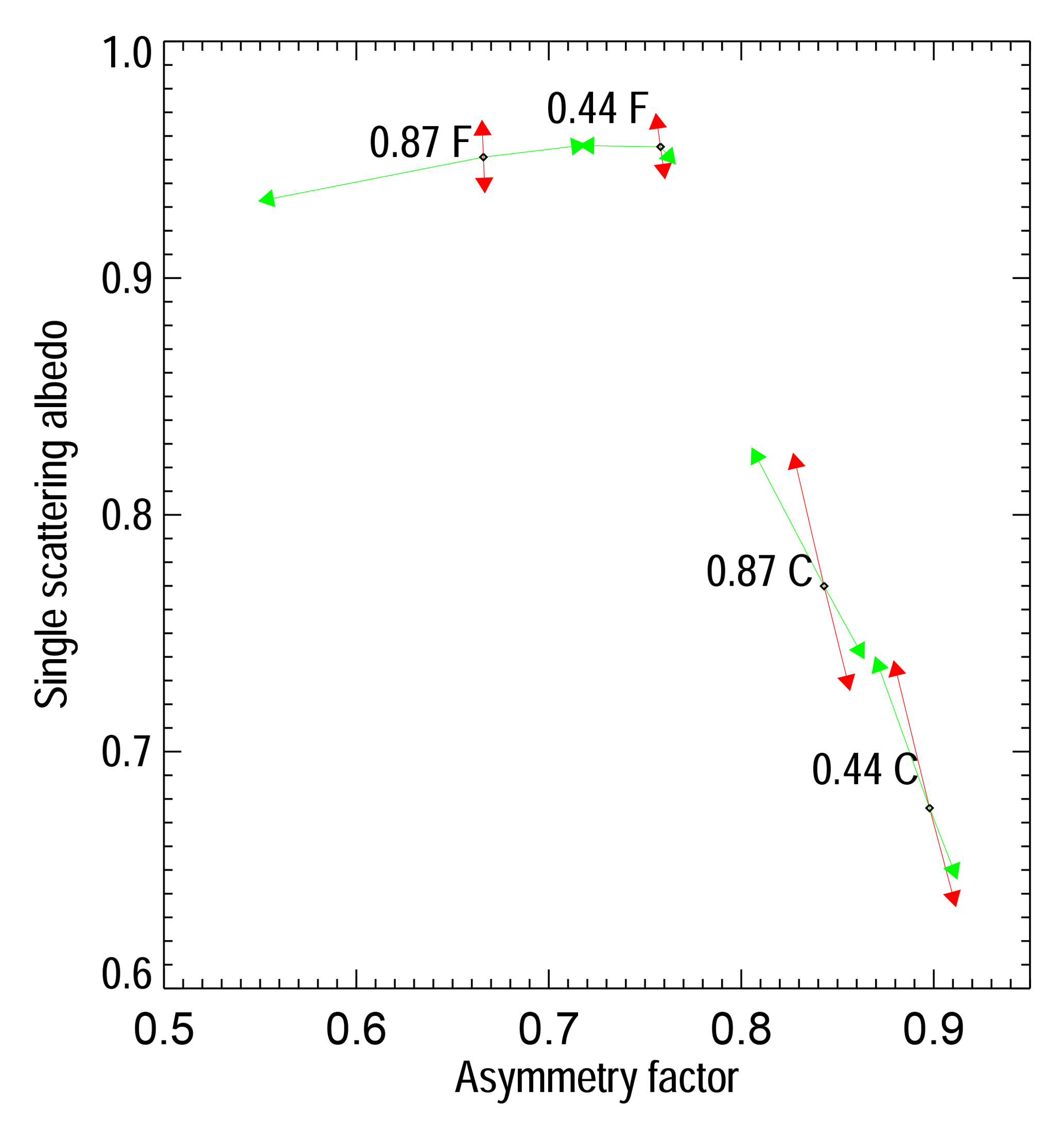
Figure 2 Example of sensitivity of aerosol single-scattering properties to particle median radius (green arrows) and imaginary part of the refractive index (red arrows) at 0.44 and 0.87 µm for fine-mode, F (r_mf=0.1 µm), and coarse mode, C (r_mc=2.0 µm). The length of the arrows reflects the magnitude of the change.

A visual inspection of Fig. 1 based on Govaerts et al. (2010b) reveals that aerosol models occupy different regions in the {g,ω₀} space according to the dominant particle size distribution, i.e. fine or coarse. Within that space, an aerosol model is defined by the spectral behaviour of the {g(λ),ω₀(λ)} pairs, where λ indicates the wavelength. The proposed fine-mode models vary mostly as a function of ω₀, which is largely determined by the imaginary part of the refractive index n_i. Conversely, aerosol models dominated by coarse particles show little dependency on g and are therefore organised parallel to the ordinate axis. The main parameter discriminating these latter models is the median radius r_m, which essentially determines the asymmetry parameter value at a given wavelength.

To illustrate the dependence of g and ω₀ on the median radius r_m (http://eodg.atm.ox.ac.uk/user/grainger/research/aerosols.pdf, last access: (9 December 2018) and imaginary part of the refractive index n_i, fine- and coarse-mono-mode aerosol models were generated with r_m=0.15 and 2.0 µm respectively. The other microphysical values have been fixed to σ_r=0.5 µm, n_r=1.42 and n_i=0.008, where σ_r is the radius standard deviation and n_r the real part of the refractive index. These values were selected to ease the explanation of the organisation of the aerosol models in Fig. 1. Black dots in Fig. 2 show the corresponding location of {g,ω₀} at 0.44 and 0.87 µm. The magnitude of the red arrows illustrate the sensitivity to a n_i change of ±0.0025 and the green ones to a r_m change of ±25 %. For the fine mono-mode (F), changes in n_i essentially translate in displacement along the ω₀ axis, while changes in r_m result in changes almost parallel to the g axis. There is also a clear relationship between the particle size and g for that mode. A change in the particle size results in a change in g, while ω₀ remains relatively unchanged. The situation is quite different for the coarse mono-mode, where changes in both n_i and r_m induce displacement parallel to the ω₀ axis with limited impact on g values.

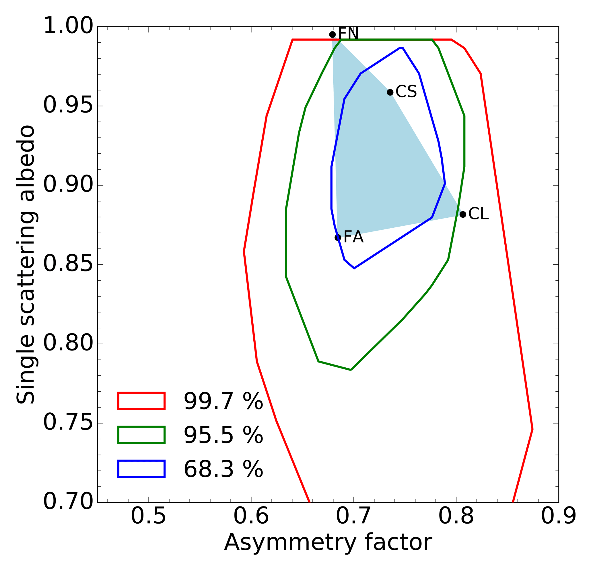
Figure 3 Example of a region (light-blue area) in the {g,ω₀} solution space at 0.44 µm defined by four aerosol vertices: single fine-mode non-absorbing (FN), single fine-mode absorbing (FA), coarse mode with small radius (CS) and coarse mode with large radius (CL). The isolines show the probability that the aerosol single-scattering properties derived from AERONET observations with the method of Dubovik et al. (2006) fall within the delineated spaces.

The actual extent of solutions in the {g,ω₀} space for a given spectral band can be outlined by a series of vertices defined by aerosol single-scattering properties (Fig. 3). Following Fig. 2, these vertices are defined by absorbing and non-absorbing fine mono-mode models with small radii of about 0.1 µm, labelled respectively FA and FN, and by two coarse mono-modes with different radii, i.e. large (1 µm) and small (0.3 µm), labelled respectively CL and CS. In Sect. 4, we will see how any pair of single-scattering albedo and phase function values can be expressed as a linear combination of the vertex properties.

The position of these vertices is critical as they should encompass the most likely aerosol single-scattering properties that could be observed at a given time and location. Different approaches could be used to define the position of these vertices. The positions can be derived from the analysis of typical aerosol single-scattering properties available in databases such as the Optical Properties of Aerosols and Clouds (OPAC) (Hess et al., 1998). Alternatively, it is also possible to follow a similar approach to the one proposed in Govaerts et al. (2010b), who analysed the single-scattering albedo and phase function values derived from AERONET observations acquired in a specific region of interest for a given period (Dubovik et al., 2006). The red isoline in Fig. 3 delineates the area [g,ω₀] of the solution space where 99.7 % of the aerosol single-scattering properties derived by Dubovik et al. (2006) from AERONET observations are located. The green and blue lines respectively show the 95 % and 68 % probability regions. These values have been derived using all available level 2 AERONET observations since 1993. Finally, the model proposed by Schuster et al. (2005) can be used to determine the spectral variations of the single-scattering properties outside the spectral bands measured by AERONET. This work relies on simulated data and the aerosol vertices have been positioned to sample the solution space in a realistic way. When processing actual satellite data over a specific region or period, it is advised to calculate the isolines corresponding to that region of interest from AERONET observations and to adjust the position of the aerosol vertices accordingly as performed in Part 2.

4 Forward radiative transfer model

4.1 Overview

The forward model, named FASTRE, simulates the TOA bidirectional reflectance factor (BRF) $y_m(\mathbf{x},\mathbf{b};\mathbf{m})$ as a function of the independent parameters m defining the observation conditions and a series of state variables x describing the state of the atmosphere and underlying surface. Model parameters b represent variables such as total column water vapour that influence the value of $y_m(\mathbf{x},\mathbf{b};\mathbf{m})$ but cannot be retrieved from the processed space-based observations due to the lack of information. The independent parameters m include the illumination and viewing geometries (Ω₀,Ω_v) and the wavelength dependence. The RTE is solved with the matrix operator method (Fischer and Grassl, 1984) optimised by Liu and Ruprecht (1996) for a limited number of quadrature points.

The model simulates observations acquired within spectral bands $\stackrel{\mathrm{̃}}{\mathit{\lambda }}$ characterised by their spectral response. Gaseous transmittances in these bands are precomputed and stored in LUTs. The model computes the contributions from single and multiple scattering separately, the latter being solved in Fourier space. In order to reduce the computation time, the forward model relies on the same atmospheric vertical structure as in Govaerts et al. (2010b), i.e. a three-level system containing two layers (Fig. 4). The lowest level, Z₀, represents the surface. The lower layer, L_a, ranging from levels Z₀ to Z_a, contains the aerosol particles. Molecular scattering and absorption also take place in that layer, which is radiatively coupled with the surface for both single and the multiple scattering. The upper layer, L_g, ranging from Z_a to Z_s, is only subject to molecular absorption.

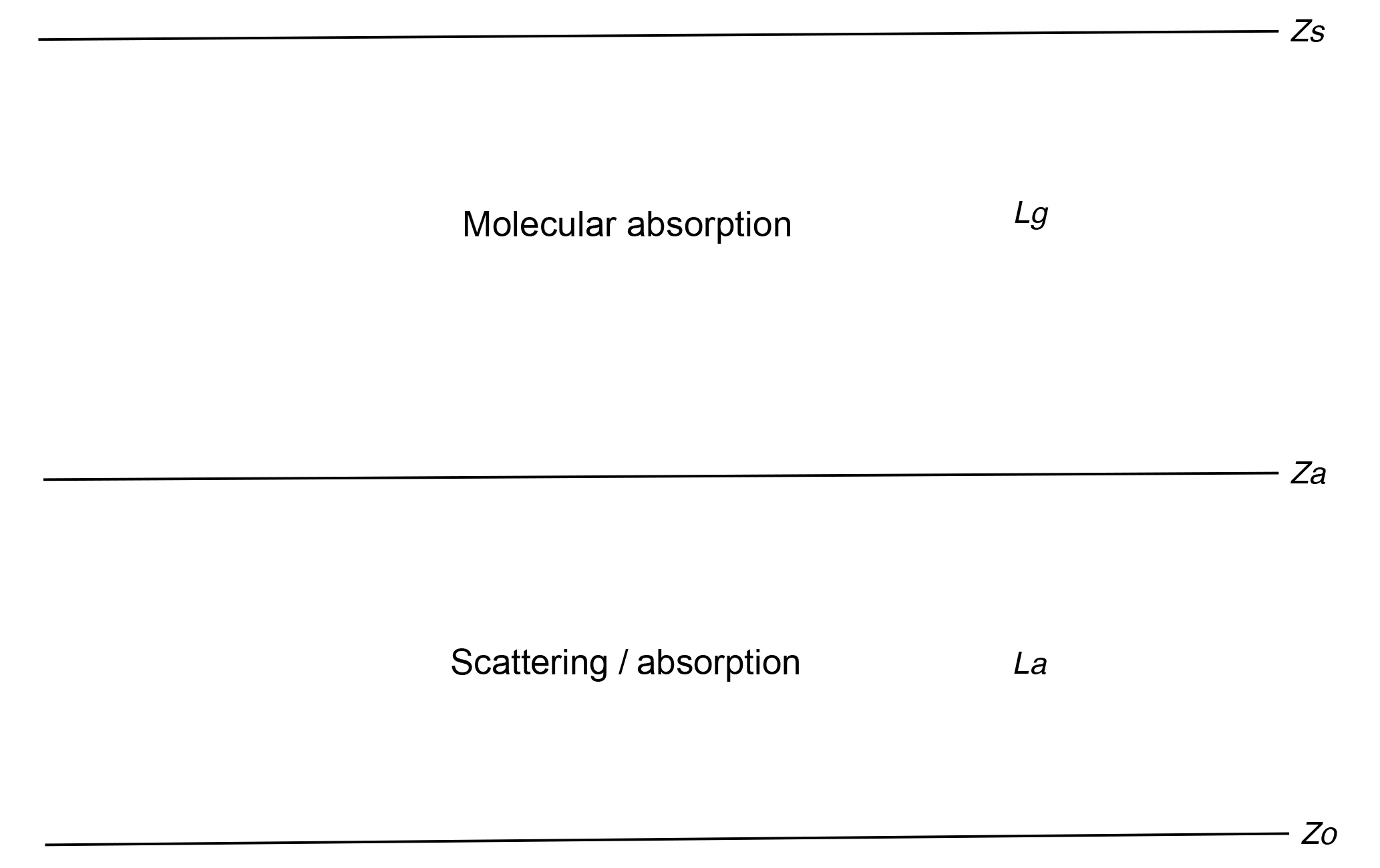
Figure 4 Atmospheric vertical structure of the FASTRE model. The surface is at level Z₀ and radiatively coupled with the lower layer L_a extending from level Z₀ to Z_a. This layer includes scattering and absorption processes. The upper layer, L_g, runs from level Z_a to Z_s and only accounts for gas absorption processes.

The surface reflectance $r_{\mathrm{s}}({\mathbf{x}}_{\mathbf{s}},\mathbf{b};\mathbf{m})$ over land is represented by the so-called RPV (Rahman–Pinty–Verstraete) model characterised by four parameters, ${\mathbf{x}}_{\mathbf{s}}=\mathit{\{}{\mathit{\rho }}_{\mathrm{0}},k,\mathrm{\Theta },{\mathit{\rho }}_c\mathit{\}}$, that are all wavelength dependent (Rahman et al., 1993). The ρ₀ parameter, included in the [0,1] interval, controls the mean amplitude of the BRF and strongly varies with wavelengths. The k parameter is the modified Minnaert's contribution that determines the bowl or bell shape of the BRF and typically varies between 0 and 2. The asymmetry parameter Θ of the Henyey–Greenstein phase function varies between −1 and 1. The ρ_c parameter controls the amplitude of the hotspot due to the “porosity” of the medium. This parameter varies between −1 and 1. For the simulations over the ocean, the Cox–Munk model (Cox and Munk, 1954) is used as implemented in Vermote et al. (1997).

Aerosol single-scattering properties in the layer L_a are represented by an external mixture of a series of predefined aerosol vertices as explained in Sect. 4.2. The L_g layer only contains absorbing gas not included in the scattering layer, such as high-altitude ozone, the part of the total column water vapour not included in layer L_a and a few well-mixed gases.

The FASTRE model expresses the TOA BRF in a given spectral band $\stackrel{\mathrm{̃}}{\mathit{\lambda }}$ as a sum of the single $I_{\mathrm{s}}^{\uparrow }$ and multiple $I_{\mathrm{m}}^{\uparrow }$ scattering contributions as in

$$\begin{array}{}\text{(1)}& y_m(\mathbf{x},\mathbf{b};\mathbf{m})=T_{L_g}(\mathbf{b};\mathbf{m}){\displaystyle \frac{I_{\mathrm{s}}^{\uparrow }(\mathbf{x},\mathbf{b};\mathbf{m})+I_{\mathrm{m}}^{\uparrow }(\mathbf{x},\mathbf{b};\mathbf{m})}{E_{\mathrm{0}}^{\downarrow }\left(\mathbf{m}\right){\mathit{\mu }}_{\mathrm{0}}}},\end{array}$$

where

• $I_{\mathrm{s}}^{\uparrow }(\mathbf{x},\mathbf{b};\mathbf{m})$ is the upward radiance field at level Z_a due to the single scattering,

• $I_{\mathrm{m}}^{\uparrow }(\mathbf{x},\mathbf{b};\mathbf{m})$ is the upward radiance field at level Z_a due to the multiple scattering,

• $T_{L_g}(\mathbf{b};\mathbf{m})$ denotes the total transmission factor in the L_g layer,

• $E_{\mathrm{0}}^{\downarrow }\left(\mathbf{m}\right)$ denotes the solar irradiance at level Z_s corrected for the Sun–Earth distance variations.

The single-scattering contribution is written

$$\begin{array}{ll}{\displaystyle }& {\displaystyle }{I}_{\mathrm{s}}^{\uparrow }(\mathbf{x},\mathbf{b};\mathbf{m})=\\ \text{(2)}& {\displaystyle }& {\displaystyle \frac{E_{\mathrm{0}}^{\downarrow }\left(\mathbf{m}\right){\mathit{\mu }}_{\mathrm{0}}}{\mathit{\pi }}}\exp \left({\displaystyle \frac{-\mathit{\tau }{}_{L_a}}{{\mathit{\mu }}_{\mathrm{0}}}}\right)r_{\mathrm{s}}({\mathbf{x}}_{\mathbf{s}},\mathbf{b};\mathbf{m})\exp \left({\displaystyle \frac{-\mathit{\tau }{}_{L_a}}{{\mathit{\mu }}_{\mathrm{v}}}}\right),\end{array}$$

where $\mathit{\tau }{}_{L_a}$ is the total optical thickness of layer L_a. μ₀ and μ_v are the cosine of the illumination and viewing zenith angles respectively.

The multiple-scattering contribution, $I_{\mathrm{m}}^{\uparrow }(\mathbf{x},\mathbf{b};\mathbf{m})$, is solved in the Fourier space for all illumination and viewing directions of the quadrature directions N_θ for 2N_θ−1 azimuthal directions. The contribution $I_{\mathrm{m}}^{\uparrow }(\mathbf{x},\mathbf{b};\mathbf{m})$ in the direction (Ω₀,Ω_v) is interpolated from the surrounding quadrature directions. Finally, the Jacobian ${\mathbf{k}}_{x_i}=\frac{\partial y_m({\mathbf{x}}_{\mathbf{i}},\mathbf{b};\mathbf{m})}{\partial x_i}$ of $y_m(\mathbf{x},\mathbf{b};\mathbf{m})$ for parameter x_i are calculated as finite differences.

4.2 Scattering layer L_a properties

The layer L_a contains a set of mono-mode aerosol models v characterised by their single-scattering properties, i.e. the single-scattering albedo ${\mathit{\omega }}_{\mathrm{0},v}\left(\stackrel{\mathrm{̃}}{\mathit{\lambda }}\right)$ and phase function ${\mathrm{\Phi }}_v(\stackrel{\mathrm{̃}}{\mathit{\lambda }},{\mathrm{\Omega }}_g)$ where Ω_g represents the scattering angle. The different vertices are combined into this layer according to their respective optical thickness ${\mathit{\tau }}_v\left(\stackrel{\mathrm{̃}}{\mathit{\lambda }}\right)$ with the total aerosol optical thickness ${\mathit{\tau }}_a\left(\stackrel{\mathrm{̃}}{\mathit{\lambda }}\right)$ of the layer being equal to

$$\begin{array}{}\text{(3)}& {\mathit{\tau }}_a\left(\stackrel{\mathrm{̃}}{\mathit{\lambda }}\right)=\sum _v{\mathit{\tau }}_v\left(\stackrel{\mathrm{̃}}{\mathit{\lambda }}\right).\end{array}$$

The phase function ${\mathrm{\Phi }}_v(\stackrel{\mathrm{̃}}{\mathit{\lambda }},{\mathrm{\Omega }}_g)$ is characterised by a limited number N_κ of Legendre coefficients equal to 2N_θ−1. The decision to use this number results from a trade-off between accuracy and computational time. When N_κ is too small, the last Legendre moment is often not equal to zero and the delta-M approximation is applied (Wiscombe, 1977). In this case, the α_d coefficient of the delta-M approximation is equal to Φ_v(N_κ). The Legendre coefficients κ_j become

$$\begin{array}{}\text{(4)}& c_j={\displaystyle \frac{{\mathit{\kappa }}_j-{\mathit{\alpha }}_d}{\mathrm{1}-{\mathit{\alpha }}_d}},\end{array}$$

and the truncated phase function is denoted by ${\mathrm{\Phi }}_v^{\prime }$. The corrected optical thickness ${\mathit{\tau }}_v^{\prime }\left(\stackrel{\mathrm{̃}}{\mathit{\lambda }}\right)$ and single-scattering albedo ${\mathit{\omega }}_{\mathrm{0},v}^{\prime }\left(\stackrel{\mathrm{̃}}{\mathit{\lambda }}\right)$ of the corresponding aerosol model become

$$\begin{array}{}\text{(5)}& {\mathit{\tau }}_v^{\prime }\left(\stackrel{\mathrm{̃}}{\mathit{\lambda }}\right)=(\mathrm{1}-{\mathit{\omega }}_{\mathrm{0},v}{\mathit{\alpha }}_d){\mathit{\tau }}_v\left(\stackrel{\mathrm{̃}}{\mathit{\lambda }}\right)\end{array}$$

and

$$\begin{array}{}\text{(6)}& {\mathit{\omega }}_{\mathrm{0},v}^{\prime }\left(\stackrel{\mathrm{̃}}{\mathit{\lambda }}\right)={\displaystyle \frac{\mathrm{1}-{\mathit{\alpha }}_d}{\mathrm{1}-{\mathit{\omega }}_{\mathrm{0},v}{\mathit{\alpha }}_d}}{\mathit{\omega }}_{\mathrm{0},v}\left(\stackrel{\mathrm{̃}}{\mathit{\lambda }}\right).\end{array}$$

The layer total optical thickness, ${\mathit{\tau }}_{L_a}$, is the sum of the gaseous, τ_g, the aerosol, ${\mathit{\tau }}_{\mathrm{a}}^{\prime }$ and the Rayleigh, τ_r, optical depth

$$\begin{array}{}\text{(7)}& {\mathit{\tau }}_{L_a}\left(\stackrel{\mathrm{̃}}{\mathit{\lambda }}\right)={\mathit{\tau }}_{\mathrm{g}}\left(\stackrel{\mathrm{̃}}{\mathit{\lambda }}\right)+{\mathit{\tau }}_{\mathrm{a}}^{\prime }\left(\stackrel{\mathrm{̃}}{\mathit{\lambda }}\right)+{\mathit{\tau }}_{\mathrm{r}}\left(\stackrel{\mathrm{̃}}{\mathit{\lambda }}\right),\end{array}$$

with ${\mathit{\tau }}_{\mathrm{a}}^{\prime }\left(\stackrel{\mathrm{̃}}{\mathit{\lambda }}\right)={\sum }_v{\mathit{\tau }}_v^{\prime }\left(\stackrel{\mathrm{̃}}{\mathit{\lambda }}\right)$. The single-scattering albedo of the scattering layer is equal to

$$\begin{array}{}\text{(8)}& {\mathit{\omega }}_{\mathrm{0}}^{\prime }\left(\stackrel{\mathrm{̃}}{\mathit{\lambda }}\right)={\displaystyle \frac{{\sum }_c{\mathit{\omega }}_{\mathrm{0},v}^{\prime }\left(\stackrel{\mathrm{̃}}{\mathit{\lambda }}\right){\mathit{\tau }}_v^{\prime }\left(\stackrel{\mathrm{̃}}{\mathit{\lambda }}\right)}{{\mathit{\tau }}_{\mathrm{a}}^{\prime }\left(\stackrel{\mathrm{̃}}{\mathit{\lambda }}\right)}}\end{array}$$

and the layer average phase function

$$\begin{array}{}\text{(9)}& {\mathrm{\Phi }}^{\prime }(\stackrel{\mathrm{̃}}{\mathit{\lambda }},{\mathrm{\Omega }}_g)={\displaystyle \frac{{\sum }_c{\mathrm{\Phi }}_v^{\prime }(\stackrel{\mathrm{̃}}{\mathit{\lambda }},{\mathrm{\Omega }}_g){\mathit{\tau }}_v^{\prime }\left(\stackrel{\mathrm{̃}}{\mathit{\lambda }}\right)}{{\mathit{\tau }}_{\mathrm{a}}^{\prime }\left(\stackrel{\mathrm{̃}}{\mathit{\lambda }}\right)}}.\end{array}$$

4.3 Gaseous layer properties

It is assumed that only molecular absorption takes place in layer L_g. The height of level Z_a is used to partition the total column water vapour and ozone concentration in each layer assuming a US76 standard atmosphere vertical profile. This height is not retrieved and is therefore a model parameter of FASTRE, which should be derived from some climatological values. $T_{L_g}$ denotes the total transmission of that layer.

Table 1 Relative bias and root mean square error in percentage between FASTRE and the reference RTM in various spectral bands.

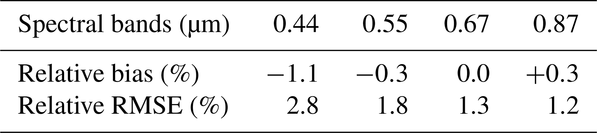
4.4 FASTRE model accuracy

The simple atmospheric vertical structure composed of two layers is the principal assumption of the FASTRE model. In order to evaluate the accuracy of FASTRE, a similar procedure to that in Govaerts et al. (2010b) has been applied. The outcome of FASTRE has been evaluated against a more elaborated 1-D radiative transfer model (RTM) (Govaerts, 2006) for sun and viewing angles varying from 0 to 70^∘, for various types of aerosols, surface reflectance and total column water vapour values. This reference RTM represents the vertical structure of the atmosphere with 50 layers. The mean relative bias and relative root mean square error (RMSE) between the reference model and FASTRE have been estimated in the main spectral bands used for aerosol retrievals. The relative RMSE, R_r, is estimated as

$$\begin{array}{}\text{(10)}& R_{\mathrm{r}}=\sqrt{{\displaystyle \frac{\mathrm{1}}{N}}\sum _N{\left({\displaystyle \frac{y_m(\mathbf{x},\mathbf{b};\mathbf{m})-y_{\mathrm{r}}(\mathbf{x},\mathbf{b};\mathbf{r})}{y_{\mathrm{r}}(\mathbf{x},\mathbf{b};\mathbf{r})}}\right)}^{\mathrm{2}}},\end{array}$$

where $y_{\mathrm{r}}(\mathbf{x},\mathbf{b};\mathbf{m})$ is the TOA BRF calculated with the reference model. In this paper, the FASTRE model solves the RTE using 16 quadrature points N_θ, which provides a good compromise between speed and accuracy. Results are shown in Table 1. The relative RMSE between FASTRE and the reference model is typically in the range of 1 %–3 %. Another comparison of FASTRE has been made against actual Project for On-Board Autonomy-Vegetation (PROBA-V) observations (Luffarelli et al., 2017). These comparisons show an RMSE in the range [0.024–0.038].

5 Inversion process

5.1 Overview

Surface reflectance characterisation requires multi-angular observations ${\mathbf{y}}_{\mathrm{\Omega }\stackrel{\mathrm{̃}}{\mathrm{\Lambda }}}$, the acquisition of which can take between several minutes, as is the case for the Multi-angle Imaging SpectroRadiometer (MISR) instrument, and several days, as is the case for the Ocean and Land Colour Instrument (OLCI) on board Sentinel-3 or the Moderate Resolution Imaging Spectroradiometer (MODIS). In the former case, data are often assumed to be acquired almost instantaneously, i.e. with the atmospheric properties remaining unchanged during the acquisition time. Such a situation considerably reduces the calculation time required to solve the RTE, as the multiple scattering term $I_{\mathrm{m}}^{\uparrow }(\mathbf{x},\mathbf{b};\mathbf{m})$ needs to be estimated only once per spectral band. In the latter case, atmospheric properties cannot be assumed to be invariant and the multiple scattering contribution needs to be solved for each observation. When geostationary observations are processed, the accumulation period is often reduced to 1 day, and the assumption that the atmosphere does not change can be converted into an equivalent radiometric uncertainty (Govaerts et al., 2010b). Strictly speaking, it should be assumed that atmospheric properties have changed when the accumulation time exceeds several minutes (Luffarelli et al., 2016).

The retrieved state variables in each spectral band $\stackrel{\mathrm{̃}}{\mathit{\lambda }}$ are composed of the x_s parameters characterising the state of the surface and the set of aerosol optical thicknesses τ_v for the aerosol vertices that are mixed in layer L_a. Prior information consists of the expected values x_b of the state variables x characterising the surface and the atmosphere on one side, and regularisation of the spectral and/or temporal variability of τ_v on the other side. Uncertainty matrices S_x are assigned to this prior information. Finally, uncertainties in the measurements S_y are assumed to be normally distributed with zero mean. The inversion process of the FASTRE model will be herein referred to as the Combined Inversion of Surface and AeRosol (CISAR) algorithm.

5.2 Cost function

The fundamental principle of OE is to maximise the probability $P=P\left(\mathbf{x}\right|{\mathbf{y}}_{\mathrm{\Omega }\stackrel{\mathrm{̃}}{\mathrm{\Lambda }}},{\mathbf{x}}_{\mathbf{b}},\mathbf{b})$ with respect to the values of the state vector x, conditional to the value of the measurements and any prior information. The conditional probability takes on the quadratic form (Rodgers, 2000):

$$\begin{array}{ll}{\displaystyle }P\left(\mathbf{x}\right)\propto & {\displaystyle }\exp \left[-\left(y_m\right(\mathbf{x},\mathbf{b};\mathbf{m})-{\mathbf{y}}_{\mathrm{\Omega }\stackrel{\mathrm{̃}}{\mathrm{\Lambda }}}{)}^T{\mathbf{S}}_y^{-\mathrm{1}}(y_m(\mathbf{x},\mathbf{b};\mathbf{m})-{\mathbf{y}}_{\mathrm{\Omega }\stackrel{\mathrm{̃}}{\mathrm{\Lambda }}})\right]+\\ {\displaystyle }& {\displaystyle }\exp \left[-(\mathbf{x}-{\mathbf{x}}_b{)}^T{\mathbf{S}}_x^{-\mathrm{1}}(\mathbf{x}-{\mathbf{x}}_b)\right]+\\ {\displaystyle }& {\displaystyle }\exp \left[-{\mathbf{x}}^T{\mathbf{H}}_a^T{\mathbf{S}}_a^{-\mathrm{1}}{\mathbf{H}}_a\mathbf{x}\right]+\\ \text{(11)}& {\displaystyle }& {\displaystyle }\exp \left[-{\mathbf{x}}^T{\mathbf{H}}_l^T{\mathbf{S}}_l^{-\mathrm{1}}{\mathbf{H}}_l\mathbf{x}\right],\end{array}$$

where the first two terms represent weighted deviations from measurements and the prior state parameters respectively, the third represents the AOT temporal smoothness constraints and the fourth represents the AOT spectral constraint, with respective uncertainty matrices S_a and S_l. The algorithm proposed by Dubovik et al. (2011) implements similar temporal and spectral smoothness constraints. The two matrices H_a and H_l, representing respectively the temporal and spectral constraints, can be written as block diagonal matrices:

$$\begin{array}{}\text{(12)}& \mathbf{H}=\left(\begin{array}{ccccc}{\mathbf{H}}^{{\mathit{\rho }}_{\mathrm{0}}}& \mathbf{0}& \mathbf{0}& \mathbf{0}& \mathbf{0}\\ \mathbf{0}& {\mathbf{H}}^k& \mathbf{0}& \mathbf{0}& \mathbf{0}\\ \mathbf{0}& \mathbf{0}& {\mathbf{H}}^{\mathit{\theta }}& \mathbf{0}& \mathbf{0}\\ \mathbf{0}& \mathbf{0}& \mathbf{0}& {\mathbf{H}}^{{\mathit{\rho }}_c}& \mathbf{0}\\ \mathbf{0}& \mathbf{0}& \mathbf{0}& \mathbf{0}& {\mathbf{H}}^{\mathit{\tau }}\end{array}\right),\end{array}$$

where the four blocks ${\mathbf{H}}^{{\mathit{\rho }}_{\mathrm{0}}}$, H^k, H^θ and ${\mathbf{H}}^{{\mathit{\rho }}_c}$ express the spectral constraints between the surface parameters. Their values are set to zero when these constraints are not active. The submatrix ${\mathbf{H}}_a^{\mathit{\tau }}$ can also be written using blocks ${\mathbf{H}}_{a;\stackrel{\mathrm{̃}}{\mathit{\lambda }},v}^{\mathit{\tau }}$ along the diagonal. For a given spectral band $\stackrel{\mathrm{̃}}{\mathit{\lambda }}$ and aerosol vertex v, the block ${\mathbf{H}}_{a;\stackrel{\mathrm{̃}}{\mathit{\lambda }},v}^{\mathit{\tau }}$ is defined as follows:

$$\begin{array}{}\text{(13)}& {\mathbf{H}}_{a;\stackrel{\mathrm{̃}}{\mathit{\lambda }},v}^{\mathit{\tau }}{\mathit{\tau }}_{\stackrel{\mathrm{̃}}{\mathit{\lambda }},v}=\left(\begin{array}{ccccc}\mathrm{1}& -\mathrm{1}& \mathrm{0}& \mathrm{\dots }& \mathrm{\dots }\\ \mathrm{0}& \mathrm{1}& -\mathrm{1}& \mathrm{0}& \mathrm{\dots }\\ \mathrm{\dots }& \mathrm{\dots }& \mathrm{\dots }& \mathrm{\dots }& \mathrm{\dots }\\ \mathrm{\dots }& \mathrm{\dots }& \mathrm{\dots }& \mathrm{1}& -\mathrm{1}\\ \mathrm{\dots }& \mathrm{\dots }& \mathrm{\dots }& \mathrm{\dots }& \mathrm{0}\end{array}\right)\left(\begin{array}{c}{\mathit{\tau }}_{\stackrel{\mathrm{̃}}{\mathit{\lambda }},v,\mathrm{1}}\\ {\mathit{\tau }}_{\stackrel{\mathrm{̃}}{\mathit{\lambda }},v,\mathrm{2}}\\ \mathrm{⋮}\\ {\mathit{\tau }}_{\stackrel{\mathrm{̃}}{\mathit{\lambda }},v,N_t-\mathrm{1}}\\ {\mathit{\tau }}_{\stackrel{\mathrm{̃}}{\mathit{\lambda }},v,\mathrm{1},N_t}\end{array}\right).\end{array}$$

In the same way, the submatrix ${\mathbf{H}}_l^{\mathit{\tau }}$ can be written using blocks ${\mathbf{H}}_{l;v,t}^{\mathit{\tau }}$. For a given aerosol vertex v and time t, the block ${\mathbf{H}}_{l;v,t}^{\mathit{\tau }}$ is defined as follows:

$$\begin{array}{}\text{(14)}& {\mathbf{H}}_{l;v,t}^{\mathit{\tau }}{\mathit{\tau }}_{v,t}=\left(\begin{array}{ccccc}\mathrm{0}& \mathrm{0}& \mathrm{0}& \mathrm{\dots }& \mathrm{0}\\ -\frac{{\mathit{ϵ}}_{\mathrm{2}}}{{\mathit{ϵ}}_{\mathrm{1}}}& \mathrm{1}& \mathrm{0}& \mathrm{\dots }& \mathrm{0}\\ \mathrm{0}& -\frac{{\mathit{ϵ}}_{\mathrm{3}}}{{\mathit{ϵ}}_{\mathrm{2}}}& \mathrm{1}& \mathrm{\dots }& \mathrm{0}\\ \mathrm{\dots }& \mathrm{\dots }& \mathrm{\dots }& \mathrm{\ddots }& \mathrm{0}\\ \mathrm{\dots }& \mathrm{\dots }& \mathrm{\dots }& -\frac{{\mathit{ϵ}}_{N_{\mathit{\lambda }}}}{{\mathit{ϵ}}_{N_{\mathit{\lambda }}-\mathrm{1}}}& \mathrm{1}\end{array}\right)\left(\begin{array}{c}{\mathit{\tau }}_{\mathrm{1},v,t}\\ {\mathit{\tau }}_{\mathrm{2},v,t}\\ {\mathit{\tau }}_{\mathrm{3},v,t}\\ \mathrm{⋮}\\ {\mathit{\tau }}_{N_{\stackrel{\mathrm{̃}}{\mathit{\lambda }}},v,t}\end{array}\right),\end{array}$$

where the ϵ_l represents the uncertainties associated with the AOT spectral constraints of the individual vertex v, bounding the solution space. The spectral variations of τ_v between band ${\stackrel{\mathrm{̃}}{\mathit{\lambda }}}_l$ and ${\stackrel{\mathrm{̃}}{\mathit{\lambda }}}_{l+\mathrm{1}}$ are assumed to vary, as

$$\begin{array}{}\text{(15)}& {\displaystyle \frac{{\mathit{\tau }}_{{\stackrel{\mathrm{̃}}{\mathit{\lambda }}}_l,v}}{{\mathit{\tau }}_{{\stackrel{\mathrm{̃}}{\mathit{\lambda }}}_{l+\mathrm{1}},v}}}={\displaystyle \frac{e_{{\stackrel{\mathrm{̃}}{\mathit{\lambda }}}_l}}{e_{{\stackrel{\mathrm{̃}}{\mathit{\lambda }}}_{l+\mathrm{1}}}}},\end{array}$$

where $e_{{\stackrel{\mathrm{̃}}{\mathit{\lambda }}}_l}$ is the extinction coefficient in band ${\stackrel{\mathrm{̃}}{\mathit{\lambda }}}_l$.

Maximising the probability function in Eq. (11) is equivalent to minimising the negative logarithm

$$\begin{array}{}\text{(16)}& J\left(\mathbf{x}\right)=J_y\left(\mathbf{x}\right)+J_x\left(\mathbf{x}\right)+J_a\left(\mathbf{x}\right)+J_l\left(\mathbf{x}\right),\end{array}$$

with

$$\begin{array}{}\text{(17)}& {\displaystyle }{J}_y\left(\mathbf{x}\right)& {\displaystyle }=\left(y_m\right(\mathbf{x},\mathbf{b},\mathrm{\Omega })-{\mathbf{y}}_{\mathrm{\Omega }\stackrel{\mathrm{̃}}{\mathrm{\Lambda }}}){\mathbf{S}}_y^{-\mathrm{1}}\left(y_m\right(\mathbf{x},\mathbf{b},\mathrm{\Omega })-{\mathbf{y}}_{\mathrm{\Omega }\stackrel{\mathrm{̃}}{\mathrm{\Lambda }}}{)}^T\text{(18)}& {\displaystyle }{J}_x\left(\mathbf{x}\right)& {\displaystyle }=(\mathbf{x}-{\mathbf{x}}_b){\mathbf{S}}_x^{-\mathrm{1}}(\mathbf{x}-{\mathbf{x}}_b{)}^T\text{(19)}& {\displaystyle }{J}_a\left(\mathbf{x}\right)& {\displaystyle }={\mathbf{x}}^T{\mathbf{H}}_a^T{\mathbf{S}}_a^{-\mathrm{1}}{\mathbf{H}}_a\mathbf{x}\text{(20)}& {\displaystyle }{J}_l\left(\mathbf{x}\right)& {\displaystyle }={\mathbf{x}}^T{\mathbf{H}}_l^T{\mathbf{S}}_l^{-\mathrm{1}}{\mathbf{H}}_l\mathbf{x}.\end{array}$$

Notice that the cost function J is minimised with respect to the state variable x, so that the derivative of J is independent of the model parameters b. The need for angular sampling to document the surface anisotropy leads to an unbalanced dimension of n_x and n_y with n_y>n_x, where n_y and n_x represent the number of observations and state variables respectively. According to Dubovik et al. (2006), these additional observations should improve the retrieval as, from a statistical point of view, repeating similar observations implies that the variance should decrease. Accordingly, the magnitude of the elements of the covariance matrix should decrease as $\mathrm{1}/\sqrt{n_y}$. Thus, repeating similar observations results in some enhancements of retrieval accuracy, which is proportional to the ratio n_y∕n_x. Hence, the cost function which is actually minimised is $J_s\left(\mathbf{x}\right)=J_y\left(\mathbf{x}\right)+n_y/n_x\left(J_x\right(\mathbf{x})+J_a(\mathbf{x})+J_l(\mathbf{x}\left)\right)$.

5.3 Retrieval uncertainty estimation

The retrieval uncertainty is based on the OE theory, assuming linear behaviour of $y_m(\mathbf{x},\mathbf{b};\mathbf{m})$ in the vicinity of the solution $\widehat{\mathbf{x}}$. Under this condition, the retrieval uncertainty ${\mathit{\sigma }}_{\widehat{\mathbf{x}}}$ is determined by the shape of J(x) at $\widehat{\mathbf{x}}$

$$\begin{array}{ll}{\displaystyle }& {\displaystyle }{\mathit{\sigma }}_{\widehat{\mathbf{x}}}^{\mathrm{2}}={\left({\displaystyle \frac{{\partial }^{\mathrm{2}}{J}_s\left(\mathbf{x}\right)}{\partial {\mathbf{x}}^{\mathrm{2}}}}\right)}^{-\mathrm{1}}=\\ \text{(21)}& {\displaystyle }& {\displaystyle }{\left({\mathbf{K}}_x^T{\mathbf{S}}_y^{-\mathrm{1}}{\mathbf{K}}_x+{\mathbf{S}}_x^{-\mathrm{1}}+{\mathbf{H}}_a^T{\mathbf{S}}_a^{-\mathrm{1}}{\mathbf{H}}_a+{\mathbf{H}}_l^T{\mathbf{S}}_l^{-\mathrm{1}}{\mathbf{H}}_l\right)}^{-\mathrm{1}},\end{array}$$

where K_x is the Jacobian matrix of $y_m(\mathbf{x},\mathbf{b};\mathbf{m})$ calculated in $\widehat{\mathbf{x}}$. Combining Eqs. (21) and (8), the uncertainty in the retrieval of ω₀ in band $\stackrel{\mathrm{̃}}{\mathit{\lambda }}$ is written

$$\begin{array}{}\text{(22)}& {\mathit{\sigma }}_{\widehat{{\mathit{\omega }}_{\mathrm{0}}}}^{\mathrm{2}}\left(\stackrel{\mathrm{̃}}{\mathit{\lambda }}\right)=\sum _v{\left({\displaystyle \frac{{\mathit{\omega }}_{\mathrm{0},v}\left(\stackrel{\mathrm{̃}}{\mathit{\lambda }}\right)-{\mathit{\omega }}_{\mathrm{0}}\left(\stackrel{\mathrm{̃}}{\mathit{\lambda }}\right)}{{\mathit{\tau }}_a\left(\stackrel{\mathrm{̃}}{\mathit{\lambda }}\right)}}\right)}^{\mathrm{2}}{\mathit{\sigma }}_{\widehat{{\mathit{\tau }}_v}}^{\mathrm{2}}\left(\stackrel{\mathrm{̃}}{\mathit{\lambda }}\right).\end{array}$$

A similar equation can be derived for the estimation of ${\mathit{\sigma }}_g^{\mathrm{2}}$.

5.4 Acceleration methods

The minimisation of Eq. (16) relies on an iterative approach with $y_m(\mathbf{x},\mathbf{b};\mathbf{m})$ and the associated Jacobians K_x being estimated at each iteration. In order to reduce the calculation time dedicated to the estimation of $y_m(\mathbf{x},\mathbf{b};\mathbf{m})$ and K_x, a series of methods have been implemented. All quantities that do not explicitly depend on the state variables, such as the observation conditions m, model parameters b, quadrature point weights, etc. are computed only once prior to the optimisation.

When solving the RTE, the estimation of the multiple scattering term is by far the most time-consuming step. Hence, during the iterative optimisation process, when the change $\mathrm{\Delta }{\mathit{\tau }}_a\left(\stackrel{\mathrm{̃}}{\mathit{\lambda }}\right)$ between iteration j and j+1 is small, the multiple scattering contribution at iteration j+1 is estimated with

$$\begin{array}{ll}{\displaystyle }& {\displaystyle }{I}_{\mathrm{m}}^{\uparrow }\left({\mathit{\tau }}_a\right(j+\mathrm{1},\stackrel{\mathrm{̃}}{\mathit{\lambda }}),\mathbf{b};\mathbf{m})=I_{\mathrm{m}}^{\uparrow }\left({\mathit{\tau }}_a\right(j,\stackrel{\mathrm{̃}}{\mathit{\lambda }}),\mathbf{b};\mathbf{m})\\ \text{(23)}& {\displaystyle }& {\displaystyle }+{\displaystyle \frac{\partial I_{\mathrm{m}}^{\uparrow }\left({\mathit{\tau }}_a\right(j,\stackrel{\mathrm{̃}}{\mathit{\lambda }}),\mathbf{b};\mathbf{m})}{\partial {\mathit{\tau }}_a}}\mathrm{\Delta }{\mathit{\tau }}_a\left(\stackrel{\mathrm{̃}}{\mathit{\lambda }}\right).\end{array}$$

This approximation is not used in two successive iterations to avoid inaccurate results, and the single-scattering contribution is always explicitly estimated.

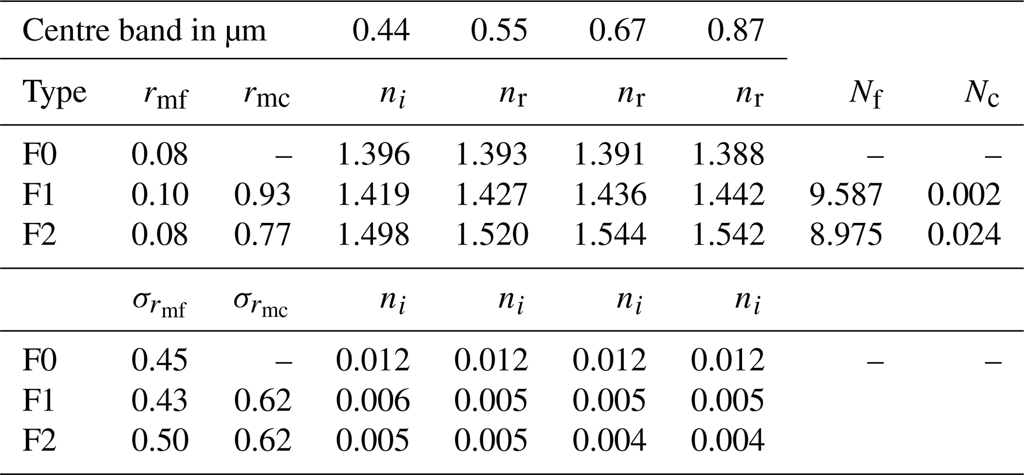
Table 2 List of aerosol properties used for the simulations. The parameters r_mf and r_mc are the median fine- and coarse-mode radii expressed in µm. Their respective standard deviations are ${\mathit{\sigma }}_{r_{\mathrm{mf}}}$ and ${\mathit{\sigma }}_{r_{\mathrm{mc}}}$. The parameters n_r and n_i are the real and imaginary part of the refractive index in the indicated bands. N_f and N_c are the fine- and coarse-mode particle concentration in number of particles per cm³.

6 Algorithm performance evaluation

6.1 Experimental set-up

A simple experimental set-up based on simulated data has been defined to illustrate the performance of the CISAR algorithm as a function of the chosen solution space. More specifically, the capability of CISAR to continuously sample the {g,ω₀} solution space is examined in detail. For the sake of simplicity, a noise-free multi-angular observation vector, ${\mathbf{y}}_{\mathrm{\Omega }\stackrel{\mathrm{̃}}{\mathrm{\Lambda }}}$, where Ω expresses the illumination and viewing geometries, is assumed to be acquired instantaneously in the principal plane and in the spectral bands listed in Table 1. A radiometric uncertainty of 3 % is assumed to compose S_y. In this ideal configuration, the solar zenith angle (SZA) is set to 30^∘. In these experiments, to concentrate on the retrieval of aerosol properties, the surface parameters prior values are set to the true values used in the simulation (Table 5) with an ascribed uncertainty of 0.03. The first guess values are randomly chosen within this uncertainty interval. Part 2 explains how prior information on the surface parameters can be derived. No prior information is assumed for the aerosol optical thickness; i.e. the prior uncertainty is set to very large values. Only regularisation of the spectral variations of τ_a is applied.

Table 3 Microphysical parameter values for the four vertices (FA, FN, CS and CL) in the selected spectral bands. Radius are given in µm.

The CISAR algorithm performance evaluation is based on a series of experiments corresponding to different selections of aerosol properties, both for the forward simulation of the observations and their inversion. Three different aerosol models are used in the forward simulations: F0, which only contains fine-mode; F1, which contains a dual-mode particle size distribution dominated by small particles; and F2, composed of a dual-mode distribution dominated by the coarse particles. Table 2 contains the values of the size distribution and refractive indices of these aerosol models. Values for the four vertices (FA, FN, CL and CS) enclosing the solution space as illustrated in Fig. 3 are given in Table 3. When the observations simulated with aerosol types F0, F1 or F2 are inverted, the list of vertices actually used depends on the type of experiment as indicated in Table 4. For all these scenarios, an AOT of 0.4 at 0.55 µm is assumed.

Table 4 List of experiments: the names are provided in the first column. The active vertices in each experiment are indicated with the × symbol. The last column indicates the name of the aerosol model used to simulate the observations.

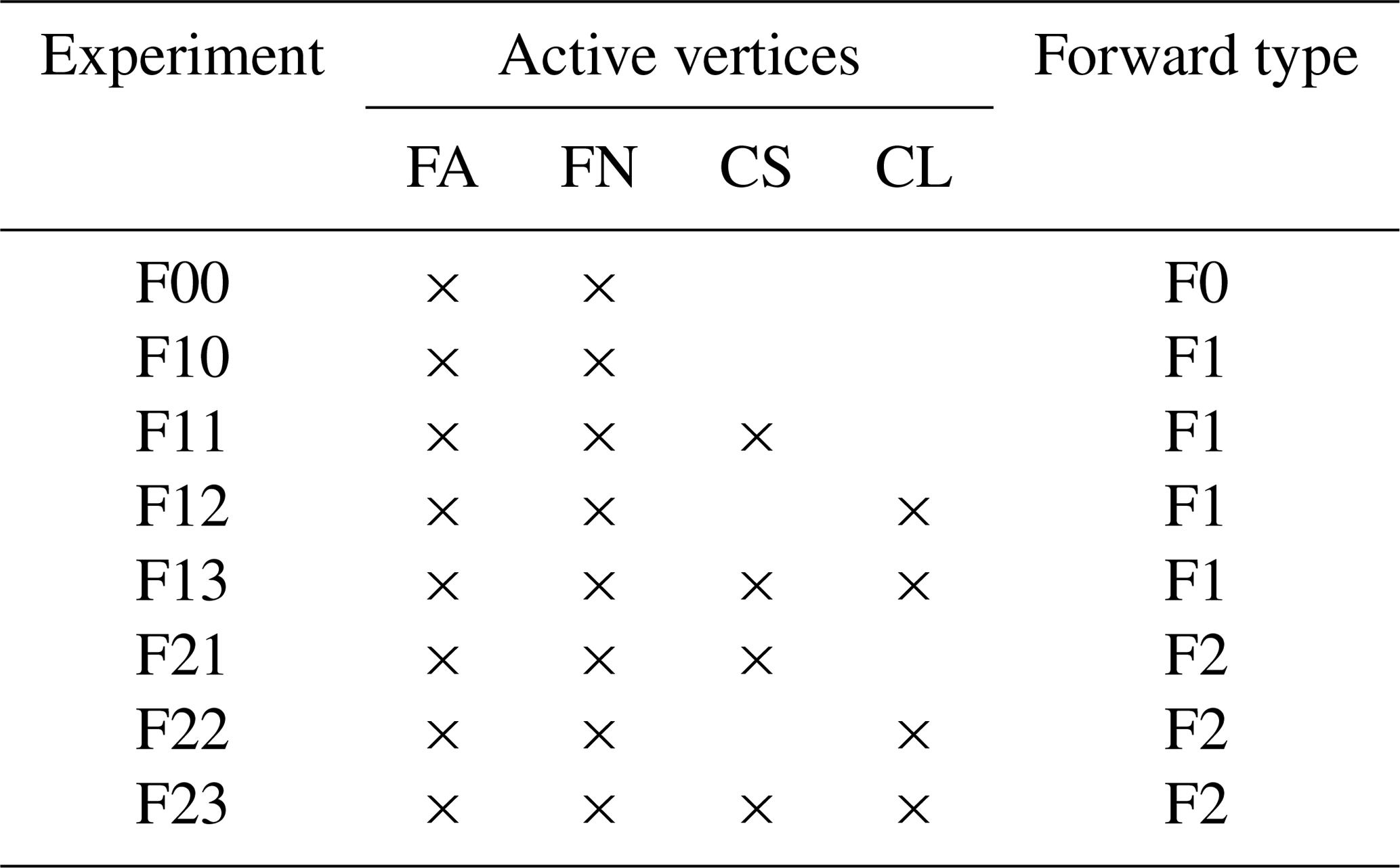
Table 5 Values of the true and retrieved surface RPV parameters for experiment F00. Wavelengths are given in µm.

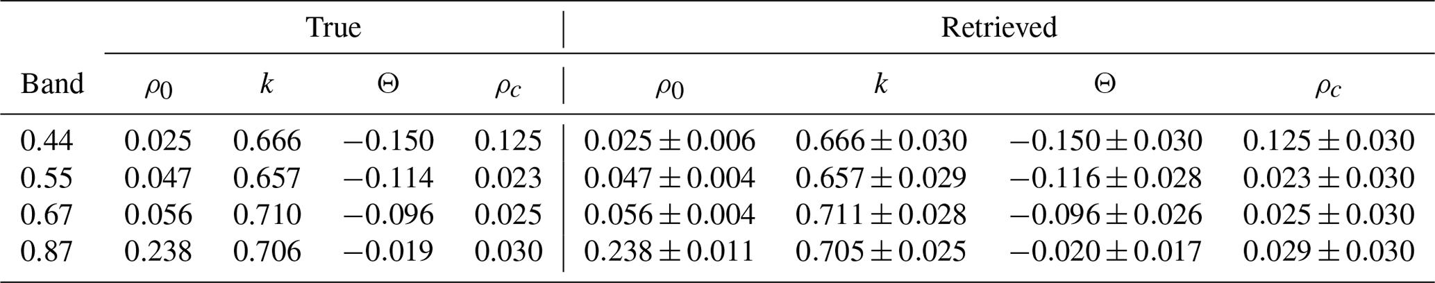
Table 6 Retrieved AOT error and uncertainties for the six experiments. The error ϵ_τ is calculated as the difference between the retrieved and the true values, δ_τ is the relative error in percent and σ_τ is the retrieval uncertainty estimated with Eq. (21). Wavelengths are given in µm.

Values used for the RPV parameters in the four selected bands are indicated in Table 5. They correspond to typical BRF values that would be observed over a vegetated surface with a leaf area index value of 3 and a bright underlying soil.

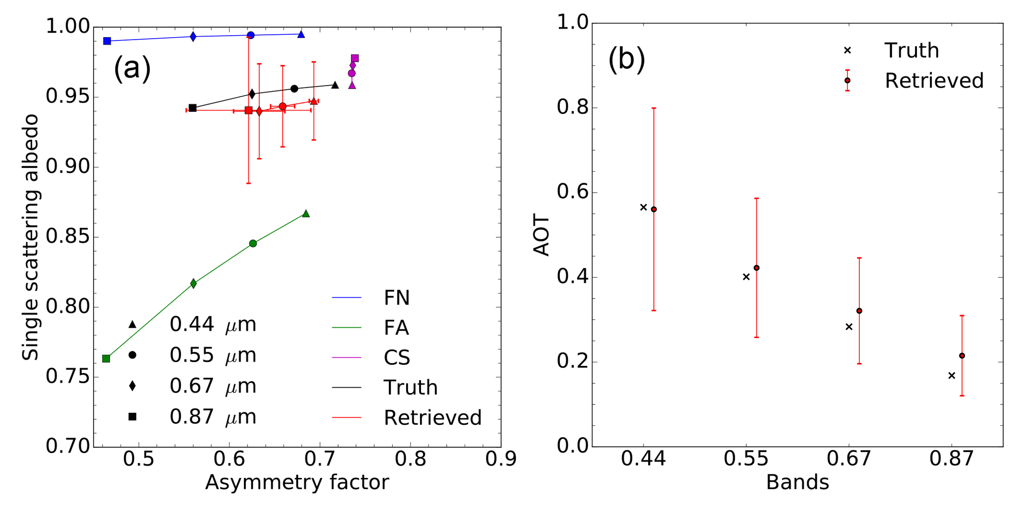
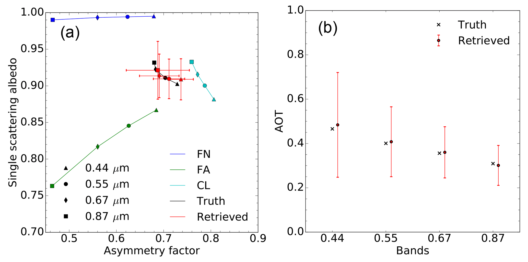
Figure 5 (a) Results of experiment F00 in the {g,ω₀} space. The aerosol vertices used for the inversion are FN (blue) and FA (green). The forward aerosol properties are shown in black and the retrieved ones in red. Vertical and horizontal red bars indicate the uncertainty of the retrieved values. (b) Retrieved AOT (red circles). The retrieval uncertainty is shown with the vertical red lines. True values are indicated with black crosses. True and retrieved values are slightly staggered to ease the reading.

Figure 6 Same as Fig. 5 but for experiment F10.

6.2 Results

6.2.1 Experiment F00

The purpose of the first experiment (F00) is to demonstrate that the CISAR algorithm can accurately retrieve aerosol properties in a simple situation, showing therefore that the inversion process works correctly. The F0 aerosol model used to simulate the observations is only composed of fine particles with a median radius of 0.08 µm, i.e. the same value as for the FN and FA vertices used for the inversion. Hence, the retrieval is limited to the imaginary part of the index of refraction, the real part being set to 1.4. With a retrieval configuration restricted to the use of only two vertices, the solution space for each wavelength is limited to a straight line between the two vertices.

Results are shown in Fig. 5 for the atmosphere and Table 5 for the surface. The asymmetry factor g and single-scattering albedo ω₀ are almost exactly retrieved. There is practically no uncertainty in the retrieval of g because of the constraints imposed by the fact that the particle radius is the same as for the F0 aerosol model. The retrieved AOT is also in very good agreement with the true values as can be seen on the right panel. The retrieval error ϵ_τ is defined as the difference between the retrieved and the true AOT values. Results are summarised in Table 6. This first experiment demonstrates that it is possible to retrieve the properties of the aerosol model F0 as a linear combination of the vertices FA and FN when only the absorption varies, the particle median radius being constant.

A comparison between the true and retrieved values in Table 5 shows that the surface parameters are very accurately retrieved. As stated in Sect. 6.1, prior information on the magnitude of the RPV parameter is assumed to be unbiased with an uncertainty of 0.03. The corresponding posterior uncertainties exhibit a significant decrease for the ρ₀ parameter at all wavelengths. Similar behaviour is not observed for the other parameters. As explained in Wagner et al. (2010), the k and Θ parameters, controlling the surface reflectance anisotropy, are strongly correlated with the amount of atmospheric scattering. Consequently, the retrieved uncertainties decrease with increasing wavelengths, i.e. as a function of the actual AOT. Despite the observations taking place in the principal plane, the posterior uncertainty on the hot spot parameter remains equal to the prior one as a result of atmospheric scattering. This fact is attributed to the relatively high value of the true AOT, and the consequent amount of scattering attenuating the hot spot. Results for the surface parameter retrieval exhibits very similar behaviour for the other experiments and will not be shown.

6.2.2 Experiment F10

Let us now examine the case in which both r_m and n_i differ from those of the vertices used for the inversion. The aerosol type F1 is used for the forward simulation with r_mf=0.1 µm for the predominant fine mode and r_mc=0.93 µm for the coarse mode. The same aerosol vertices as in experiments F00 are used for the inversion.

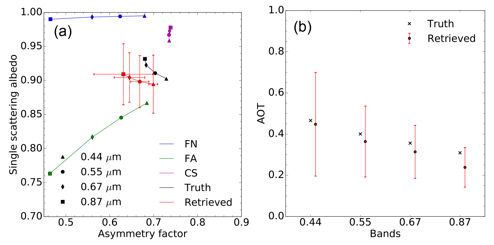
The results in Fig. 6 show that ω₀ is reasonably well retrieved unlike the g parameter, which is systematically underestimated. At any given wavelengths, it is not possible to retrieve g values outside the bounds defined by the FA and FN vertices. Consequently, the retrieved AOT values are underestimated by about 10 % (Table 6). This example illustrates the retrieval failure when the actual solution lays outside the {g,ω₀} space defined by the active vertices.

Figure 7 Same as Fig. 5 but for experiment F11.

Figure 8 Same as Fig. 5 but for experiment F12.

Figure 9 Same as Fig. 5 but for experiment F13.

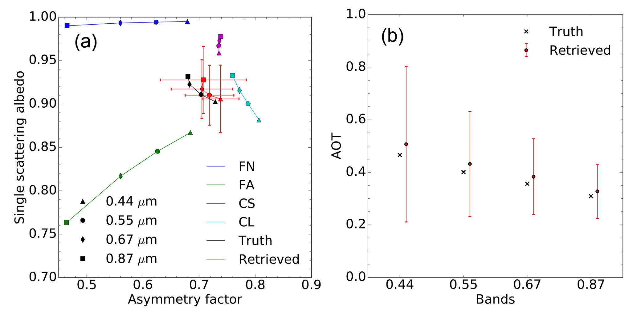
6.2.3 Experiments F11–F13

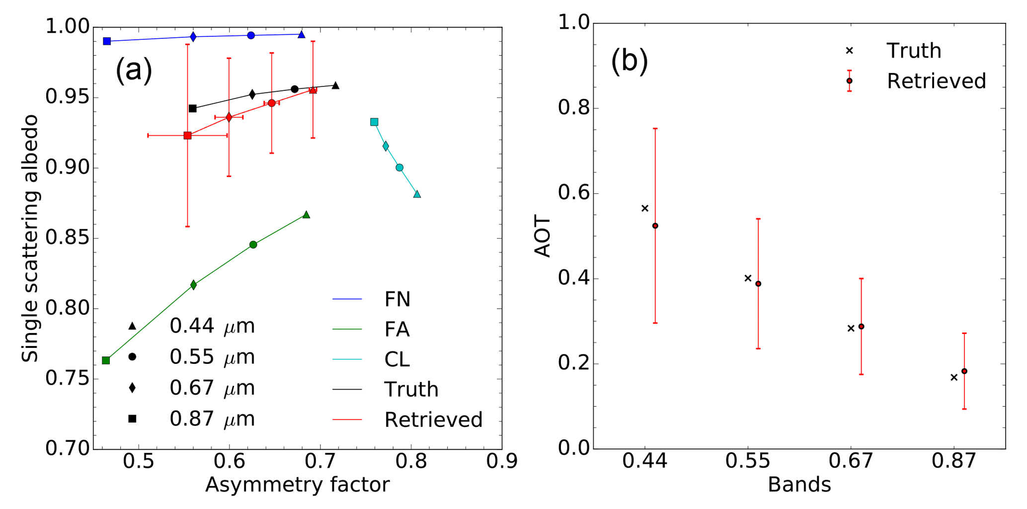
In order to improve the retrieval of the F1 aerosol model properties, the additional aerosol CS vertex with r_m=0.3 µm has been added for the inversion process. Results of experiment F11 are displayed in Fig. 7. Retrieved g values are no longer underestimated. The single-scattering albedo is slightly underestimated. It should be noted that the estimated uncertainty associated with g increases with wavelength and is particularly large at 0.87 µm, but rather underestimated at 0.44 µm. The improvement in the AOT retrieval accuracy is noticeable in the 0.44 and 0.55 µm bands where the magnitude of ϵ_r is reduced from 0.062 to 0.005 and from 0.042 to −0.021 respectively (Table 6). At larger wavelengths, the benefit of adding the CS vertex is less noticeable though the magnitude of ϵ_r remains below 0.05. Finally, the retrieval uncertainty slightly increases from 0.199 up to 0.239 for the 0.44 µm band because of the use of additional state variables τ_v associated with the inclusion of an additional vertex. Similar behaviour is observed in the other bands.

Figure 10 Same as Fig. 5 but for experiment F21.

Figure 11 Same as Fig. 5 but for experiment F22.

Figure 12 Same as Fig. 5 but for experiment F23.

For experiment F12, the CS vertex is substituted by vertex CL which has a median radius of 1.0 µm. The use of this vertex instead of CS considerably improves the retrieval of g and of ω₀ at large wavelengths (Fig. 8). As can be seen in Fig. 2, the sensitivity of aerosol single-scattering properties to particle median radius and imaginary part of the refractive index depends on the wavelength. Hence, a similar performance of the algorithm at all wavelengths should not be expected. The errors ϵ_τ in this experiment F12 are further reduced compared to experiment F11 with the exception of the 0.44 µm band. The CISAR algorithm retrieves total AODs consistent with the truth.

Finally, in experiment F13 the inversion was performed using all four vertices (Fig. 9). This additional “degree of freedom” translates into an increase of the estimated uncertainty ${\mathit{\sigma }}_{\widehat{\mathit{\tau }}}$ as a result of the large number of possible way to combine these four vertices to retrieve the properties of the aerosol model F1. In other words, using these two coarse mode vertices does not improve the characterisation of F1. The actual benefit of adding this fourth vertex, i.e. expanding the solution space, is therefore not straightforward, and it should be noted that increasing the number of vertices impacts the computational time. This series of experiments has shown that, of the four considered, the use of the FN, FA and CL vertices provides the best combination for the retrieval of aerosol model F1. With this combination, the FN and FA vertices allow for control of the amount of radiation absorbed by the aerosols, while the effects of the particle size are controlled by the CL vertex.

6.2.4 Experiments F21–F23

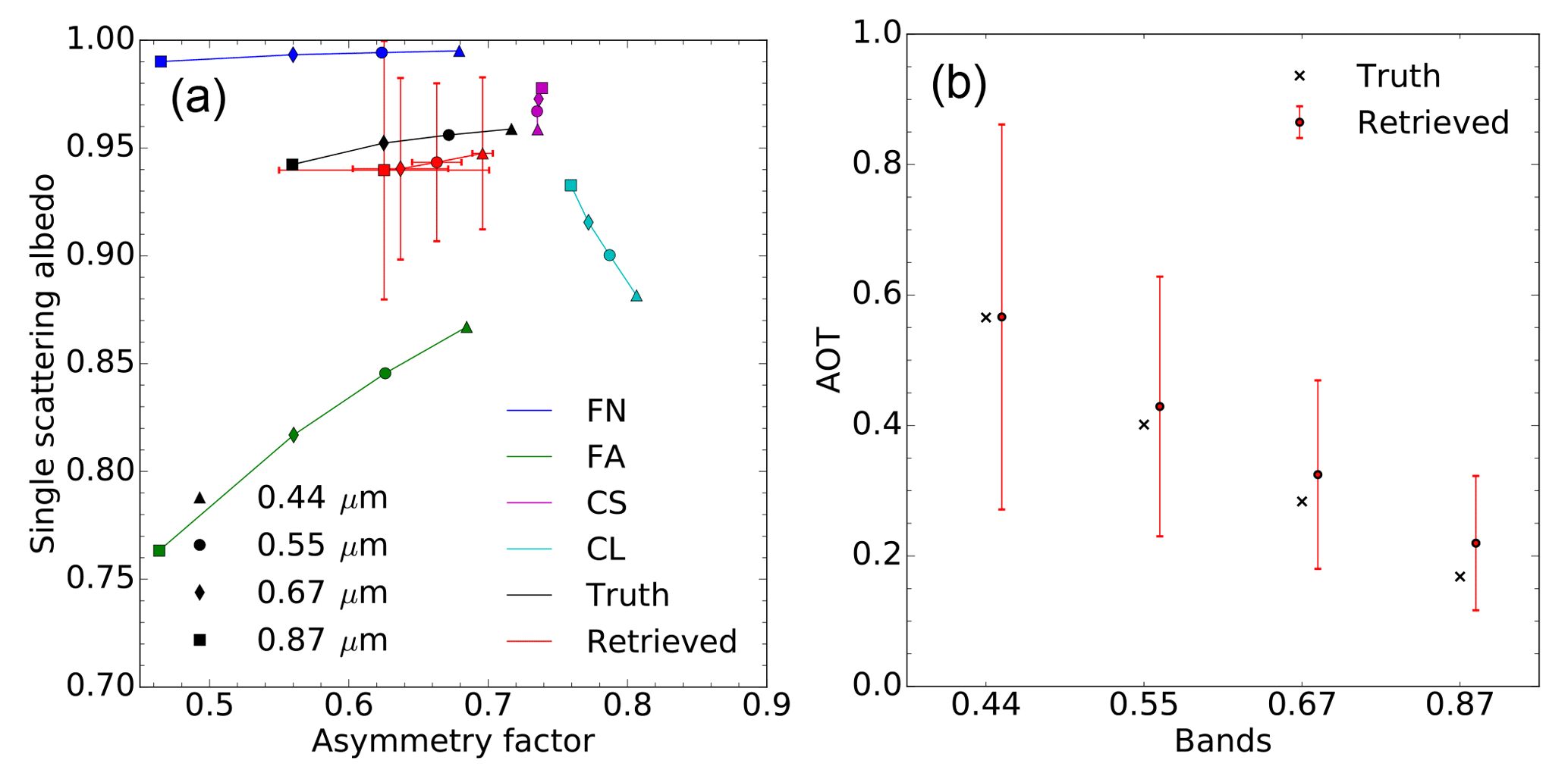
The retrieval of aerosol model F2, a dual-mode particle size distribution dominated by coarse particles, is now examined. This model is composed of a fine mode with radius r_mf=0.08 µm and a coarse mode with radius r_mc= 0.77 µm. As for the retrieval of the F1 aerosol model, three combinations of vertices have been explored, i.e. FN, FA and CS for experiment F21 (Fig. 10), FN, FA and CL for experiment F23 (Fig. 11) and FN, FA, CS and CL for experiment F22 (Fig. 11). Essentially the same conclusions hold as for the retrieval of aerosol model F1. The retrieval of the F2 model properties expressed as a linear combination of the FN, FA and CL vertices provides the best solution, with both g and ω₀ being retrieved at all wavelengths.

7 Discussion and conclusion

This paper describes the CISAR algorithm designed for the joint retrieval of surface reflectance and aerosol properties. Previous attempts to perform a joint retrieval have been reviewed, discussing their advantages and weaknesses. The limitations due to a combined used of discrete and continuous state variables in retrieval methods based on OE as in Govaerts et al. (2010b) are discussed in Sect. 2. The new method presented in this paper specifically addresses these limitations, allowing continuous variations of the aerosol single-scattering properties in the solution space without the aerosol microphysical properties explicitly appearing as state variables.

A fast-forward radiative transfer model has been designed which solves the radiative transfer equation without relying on precomputed look-up tables. This model considers two atmospheric layers. The upper layer only hosts molecular absorption. The lower layer accounts for both absorption and scattering processes due to aerosols and molecules and is radiatively coupled with the surface represented with the RPV BRF model. Single-scattering aerosol properties in this layer are expressed as a linear combination of the properties of vertices enclosing part of the solution space.

A series of different experiments has been devised to analyse the behaviour of the CISAR algorithm and its capability to retrieve aerosol single-scattering properties as well as the optical thickness. This discussion focuses on the retrieval of aerosol models dominated by the fine mode or coarse mode. These two models have pretty different spectral behaviour in the {g,ω₀} space and yet the CISAR algorithm is capable of retrieving the corresponding single-scattering properties in both cases with estimated uncertainties of about 15 %.

These experiments illustrate the possibility of using Eqs. (8) and (9) for the continuous retrieval of the aerosol single-scattering albedo and phase function. These equations assume linear behaviour of ω₀ and g in the solution space. Such assumptions have proven to be valid for the case addressed in experiment F00. This assumption is not exactly true for the retrieval aerosol models of a fine- and a coarse-particle size modes. However, the retrieved aerosol single-scattering properties are derived much more accurately than with a method based on a limited number of predefined aerosol models as in Govaerts et al. (2010b), where the single-scattering properties of only predefined models are retrieved. It thus represents a major improvement with respect to these types of retrieval approaches without requiring the use of a large number of state variables as in the method proposed by Dubovik et al. (2011), where aerosol microphysical properties are explicitly included in the set of retrieved state variables.

The choice of vertices outlining the {g,ω₀} solution space is critical. In these experiments, the best retrieval is obtained using three vertices, i.e. one vertex composed of small weakly absorbing particles (FN), one vertex composed of small absorbing particles (FA) and one vertex composed of large particles (CL). The use of a fourth vertex (CS) does not improve the retrieval and increases the estimated retrieval uncertainty.

This set of experiments represents ideal conditions, i.e. noise-free observations in the principal plane with no bias on the surface prior. This choice is motivated by the need to keep the result interpretation simple to illustrate how the new retrieval concept developed in this paper works. These experiments show the possibility of retrieving aerosol single-scattering properties within the solution space provided it is correctly bounded by the vertices. It is clear that adding noise to the observations will degrade the quality of the retrieval. Similar conclusions can hold if the observations are taking place far from the principal plane, where most of the angular variations occur. Part 2 addresses the performance of CISAR when applied to actual satellite data.