Development of an instrument for direct ozone production rate measurements: measurement reliability and current limitations

Ground-level ozone (O₃) is an important pollutant that affects both global climate change and regional air quality, with the latter linked to detrimental effects on both human health and ecosystems. Ozone is not directly emitted in the atmosphere but is formed from chemical reactions involving volatile organic compounds (VOCs), nitrogen oxides (NO_x= NO + NO₂) and sunlight. The photochemical nature of ozone makes the implementation of reduction strategies challenging and a good understanding of its formation chemistry is fundamental in order to develop efficient strategies of ozone reduction from mitigation measures of primary VOCs and NO_x emissions.

An instrument for direct measurements of ozone production rates (OPRs) was developed and deployed in the field as part of the IRRONIC (Indiana Radical, Reactivity and Ozone Production Intercomparison) field campaign. The OPR instrument is based on the principle of the previously published MOPS instrument (Measurement of Ozone Production Sensor) but using a different sampling design made of quartz flow tubes and a different O_x (O₃ and NO₂) conversion–detection scheme composed of an O₃-to-NO₂ conversion unit and a cavity attenuated phase shift spectroscopy (CAPS) NO₂ monitor. Tests performed in the laboratory and in the field, together with model simulations of the radical chemistry occurring inside the flow tubes, were used to assess (i) the reliability of the measurement principle and (ii) potential biases associated with OPR measurements.

This publication reports the first field measurements made using this instrument to illustrate its performance. The results showed that a photo-enhanced loss of ozone inside the sampling flow tubes disturbs the measurements. This issue needs to be solved to be able to perform accurate ambient measurements of ozone production rates with the instrument described in this study. However, an attempt was made to investigate the OPR sensitivity to NO_x by adding NO inside the instrument. This type of investigations allows checking whether our understanding of the turnover point between NO_x-limited and NO_x-saturated regimes of ozone production is well understood and does not require measuring ambient OPR but instead only probing the change in ozone production when NO is added. During IRRONIC, changes in ozone production rates ranging from the limit of detection (3σ) of 6.2 ppbv h⁻¹ up to 20 ppbv h⁻¹ were observed when 6 ppbv of NO was added into the flow tubes.

1 Introduction

Ground-level ozone (O₃) is a primary constituent of photochemical smog that irritates the respiratory system (WHO, 2013) and damages vegetation (Ashmore, 2005). In addition, ozone is a greenhouse gas and an important precursor of the hydroxyl radical (OH), a key species controlling the atmospheric oxidative capacity (Monks, 2005; Rohrer et al., 2014; Prinn, 2003). Ozone is a photochemical pollutant formed during daytime and has an average lifetime estimated at 22 ± 2 days (Stevenson et al., 2006), which is long enough to transport it from polluted regions to remote areas and between continents. The local production of ozone on top of the amount advected from elsewhere can lead to exceedances of air quality standards in urbanized areas, making ozone pollution an issue of global concern (Akimoto, 2003).

In the troposphere, ozone can be rapidly converted to nitrogen dioxide (NO₂) through reaction with nitric oxide (NO) and back to O₃ through NO₂ photolysis. This chemistry does not produce new ozone and is known as the O₃–NO_x photostationary state (PSS), with NO_x being the sum of NO and NO₂. The production of new ozone is driven by the oxidation of volatile organic compounds (VOCs), which leads to the production of hydroperoxy (HO₂) and organic peroxy (RO₂) radicals. The current understanding of tropospheric ozone chemistry indicates that new ozone is formed via reactions of these peroxy radicals with NO, which results in the conversion of NO to NO₂ without consumption of ozone (Monks, 2005; Seinfeld and Pandis, 2006).

When ozone is produced, reactions of peroxy radicals with NO also lead to the formation of OH, which can then oxidize other molecules of VOCs to produce more peroxy radicals and, as a consequence, more ozone. The propagation chemistry between RO_x (OH, HO₂ and RO₂) radicals, which fuels ozone production, is terminated either by NO_x–RO_x reactions or by cross reactions of RO_x radicals in NO_x-rich and NO_x-poor environments, respectively. These two types of termination reactions lead to different regimes of ozone production referred to as NO_x-limited or NO_x-saturated when the rate of ozone production increases or decreases with NO_x, respectively. The turnover point between the two regimes depends on NO_x concentrations, VOC reactivity and radical production rates (Kleinman, 2005). Since different air quality regulations have to be implemented for the two different regimes, i.e either NO_x or VOC emission regulations, investigating the sensitivity of ozone production rates (OPRs) to its precursors during field studies, such as NO_x, is important to test our understanding of the turnover point. Understanding this complex and nonlinear radical chemistry is key for the design of efficient emission control strategies.

The instantaneous ozone production rate, p(O₃), can be calculated from Eq. (1) as the rate of reactions between peroxy radicals and NO. The instantaneous ozone loss rate, l(O₃), can be calculated using Eq. (2), based on reaction rates for ozone photolysis, reactions of O₃ with HO_x and alkenes, and the reaction of OH with NO₂, since NO₂ is a reservoir molecule for O₃. The net ozone production rate, P(O₃), is then computed as the difference between instantaneous production and loss rates as shown in Eq. (3).

$$\begin{array}{ll}{\displaystyle }& {\displaystyle }p\left({\mathrm{O}}_{\mathrm{3}}\right)=k_{{\mathrm{HO}}_{\mathrm{2}}+\mathrm{NO}}\left[{\mathrm{HO}}_{\mathrm{2}}\right]\left[\mathrm{NO}\right]\\ \text{(1)}& {\displaystyle }& {\displaystyle }+\sum _i\left(k_{{\mathrm{RO}}_{\mathrm{2},i}+\mathrm{NO}}\left[{\mathrm{RO}}_{\mathrm{2}i}\right]\left[\mathrm{NO}\right]\right){\displaystyle }& {\displaystyle }l\left({\mathrm{O}}_{\mathrm{3}}\right)=k_{\mathrm{O}{(}^{\mathrm{1}}D)+{\mathrm{H}}_{\mathrm{2}}\mathrm{O}}\left[O{(}^{\mathrm{1}}D)\right]\left[{\mathrm{H}}_{\mathrm{2}}\mathrm{O}\right]+k_{\mathrm{OH}+{\mathrm{O}}_{\mathrm{3}}}\left[\mathrm{OH}\right]\left[{\mathrm{O}}_{\mathrm{3}}\right]\\ {\displaystyle }& {\displaystyle }+k_{{\mathrm{HO}}_{\mathrm{2}}+{\mathrm{O}}_{\mathrm{3}}}\left[{\mathrm{HO}}_{\mathrm{2}}\right]\left[{\mathrm{O}}_{\mathrm{3}}\right]+\sum _i{k}_{{\mathrm{O}}_{\mathrm{3}}+{\mathrm{Alkene}}_{\mathrm{i}}}\left[{\mathrm{O}}_{\mathrm{3}}\right]\left[{\mathrm{Alkene}}_i\right]\\ \text{(2)}& {\displaystyle }& {\displaystyle }+k_{\mathrm{OH}+{\mathrm{NO}}_{\mathrm{2}}}\left[\mathrm{OH}\right]\left[{\mathrm{NO}}_{\mathrm{2}}\right]\text{(3)}& {\displaystyle }& {\displaystyle }P\left({\mathrm{O}}_{\mathrm{3}}\right)=p\left({\mathrm{O}}_{\mathrm{3}}\right)-l\left({\mathrm{O}}_{\mathrm{3}}\right)\end{array}$$

Here k_X+Y is the bimolecular reaction rate constant for the two reagents X and Y. Therefore, the calculation of ozone production rates requires peroxy radical concentrations, either from ambient measurements (Green et al., 2006; Liu and Zhang, 2014; Fuchs et al., 2008; Dusanter et al., 2009a; Griffith et al., 2016) or box model outputs (Goliff et al., 2013; Stockwell et al., 2011; Saunders et al., 2003).

In most urban and suburban environments, where concentrations of NO_x are significant (10–80 ppbv), ozone production rates can reach a few tens of ppbv h⁻¹ (Mao et al., 2010). In highly polluted environments, such as Mexico City or Houston, Texas, P(O₃) can even exceed 100 ppbv h⁻¹ (Shirley et al., 2006; Chen et al., 2010). Ozone production rates lower than 10 ppbv h⁻¹ have also been observed in urban atmospheres such as Phoenix, AZ (Kleinman et al., 2002), likely due to lower initiation rates of radicals. Ozone production is usually low in more remote areas or forested environments that are not impacted by anthropogenic activities (less than 2–3 ppbv h⁻¹), due to the low NO_x concentrations (Geng et al., 2011). However, if NO_x emission sources are located downwind of a forested area, highly reactive biogenic VOCs (e.g., isoprene) can lead to an enhancement of ozone production (Geng et al., 2011; Thornton et al., 2002).

Some studies performed in urban and suburban areas, whose objectives were to test our understanding of the radical chemistry by contrasting measurements and model simulations of HO_x concentrations, showed that models tend to underestimate HO₂ for NO mixing ratios higher than a few ppbv (Ren et al., 2003, 2013; Chen et al., 2010; Dusanter et al., 2009b; Kanaya et al., 2007). In contrast, models tend to overestimate HO₂ in forested areas and regions characterized by large concentrations of biogenic VOCs (Griffith et al., 2013; Mao et al., 2012; Pugh et al., 2010). Disagreements are also present in the modeling of OH, with the models underestimating the measurements at forested environments (Lelieveld et al., 2008; Tan et al., 2001; Whalley et al., 2011; Hofzumahaus et al., 2009; Lu et al., 2013; Pugh et al., 2010), while the agreement may be better when colder temperatures lead to lower concentrations of isoprene and other VOCs (Griffith et al., 2013). The discrepancies between models and measurements question our ability to successfully measure radical species or indicate that there are still unknowns in our understanding of the radical and ozone production chemistry, which in turn could lead to erroneous P(O₃) calculations by atmospheric models. These models are widely used for the design of air quality regulations (Rao et al., 2010; Fu et al., 2006) based on emission control strategies. It is therefore essential to ensure that chemical mechanisms used in atmospheric models are accurate enough to simulate the oxidative capacity of the atmosphere and to predict both absolute rates of ozone production and the turnover point between the two ozone production regimes.

In order to address these issues, an instrument for direct ozone production measurements (MOPS) was developed by Cazorla and Brune (2010). The principle of MOPS is based on differential ozone measurements between two sampling chambers made of FEP (fluorinated ethylene propylene), one exposed to sunlight (referred to as the sampling chamber) to get an ozone production rate inside the chamber that mimics atmospheric P(O₃) and the other one covered with a UV filter (reference chamber) to suppress the radical chemistry and, as a consequence, ozone production. The difference in ozone between the two chambers divided by the exposure time yields the ozone production rate. However, NO₂ can act as a reservoir molecule for O₃ due to the rapid interconversion between these two species, and NO₂ has to be converted into O₃ before measuring ozone. The differential O_x (O_x= O₃+ NO₂) measurements yield P(O_x) values, which represent P(O₃) when NO₂ is efficiently photolyzed during daytime.

The first version of the MOPS instrument was tested on the campus of Pennsylvania State University in the late summer of 2008. These tests demonstrated the feasibility of the MOPS technique, as the instrument responded to the presence of solar radiation and ozone precursors and yielded rates of ozone production that were within a range of reasonable values (up to 10 ppbv h⁻¹) for this area. This instrument was then deployed during the Study of Houston Atmospheric Radical Precursors (SHARP, 2009) (Cazorla et al., 2012). The measurements were compared to ozone production rates calculated using measurements of HO₂ and NO (referred to as calculated P(O₃)) as well as modeled radical concentrations from a box model (referred to as modeled P(O₃)). Measured and calculated P(O₃) had similar peak values but the calculated P(O₃) tended to peak earlier in the morning when NO values were higher. Measured and modeled P(O₃) had a similar diurnal profile, but the modeled P(O₃) was only half the measured P(O₃). The MOPS deployment during the SHARP field campaign showed the potential of this instrument for contributing to the understanding of the ozone-producing chemistry but was limited by measurement uncertainties due to potential wall effects. The heterogeneous loss of NO₂ under humid conditions (RH > 50 %) was reported as a main issue for this technique.

Recently, an improved version of the MOPS instrument was deployed during the NASA's DISCOVER-AQ field campaign in 2013, in Houston, Texas (Baier et al., 2015). Wall effects were reduced by improving the design of the sampling chambers and the airflow characteristics. The measurements made over 1 month were consistent with ambient ozone observations and model-derived P(O₃) values from previous field campaigns in Houston. The authors, however, highlighted a possible bias due to surface HONO production followed by its photolysis in the sampling chamber, as well as unresolved ozone analyzer issues. HONO concentrations in the sampling chambers were reported as 2 to 5 times higher than ambient values, which could cause a bias up to 5–10 ppbv h⁻¹ on the P(O₃) measurements.

A recent publication from Sadanaga et al. (2017) also reports the development and the field deployment of another instrument to measure ozone production rates. The main differences with MOPS are the use of two quartz flow tubes instead of Teflon^® chambers, an O₃-to-NO₂ conversion unit and an NO₂ detection by laser-induced fluorescence. While quartz was chosen for the flow tubes, their inner surface is covered by a Teflon^® film. The reported detection limit is 0.5 ppbv h⁻¹ for 60 s measurements. P(O₃) values ranging from the detection limit up to 11 ppbv h⁻¹ were reported for 3 days of measurements in a forested area characterized by low mixing ratios of O₃ (< 10 ppbv) and NO_x (< 1ppbv).

In this publication, we present the development and the characterization of an ozone production rates instrument. The OPR instrument is based on the principle of the MOPS, using sampling and detection schemes similar to those proposed by Sadanaga et al. (2017). This publication describes this new instrument and its characterization in the laboratory. An emphasis is given to the modeling of the radical chemistry inside the sampling chambers to assess potential biases on P(O₃) measurements associated with instrumental characteristics and operating conditions. The publication also reports preliminary field results from the Indiana Radical, Reactivity and Ozone Production Intercomparison (IRRONIC) campaign, which highlight the current limitations of this instrument.

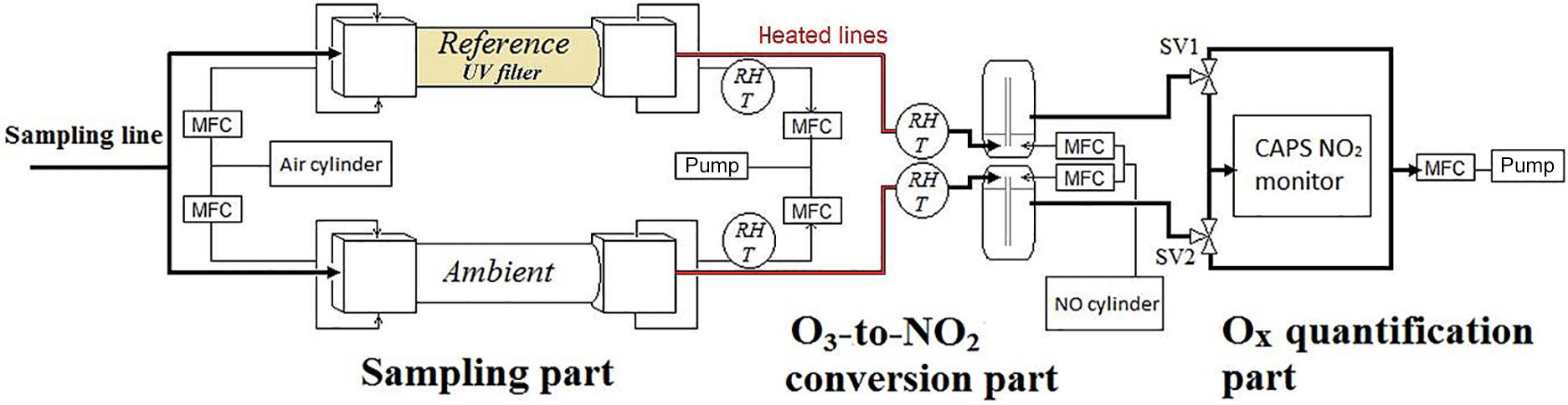
Figure 1 Schematic of the OPR instrument. O₃ converted into NO₂ by reaction with NO. Difference in O_x mixing ratios between the two flow tubes quantified by CAPS. SV: solenoid valves. MFC: mass flow controller.

2 Experimental section

2.1 Description of the OPR instrument

The principle of the OPR is based on differential O_x measurements between an ambient flow tube, exposed to sunlight to mimic ambient photochemistry, and a reference flow tube, covered with an Ultem^® film (polyetherimide, 0.25 mm thick, CS Hyde Co., USA) to block wavelengths lower than 400 nm, which in turn should suppress ozone production. As mentioned above for the MOPS instrument, the fast partitioning between O₃ and NO₂ requires measuring O_x instead of O₃, assuming that P(O₃) is equal to P(O_x) when NO₂ is efficiently photolyzed during daytime. P(O_x) is calculated from the difference in O_x between the two flow tubes, ΔO_x, divided by the mean residence time (τ) of air inside the tubes as shown in Eq. (4).

$$\begin{array}{}\text{(4)}& {\displaystyle }P\left({\mathrm{O}}_x\right)={\displaystyle \frac{\mathrm{\Delta }{\mathrm{O}}_x}{\mathit{\tau }}}={\displaystyle \frac{{\mathrm{O}}_{x_{\mathrm{amb}}}-{\mathrm{O}}_{x_{\mathrm{ref}}}}{\mathit{\tau }}}\end{array}$$

A detailed schematic of the OPR instrument is shown in Fig. 1. The two flow tubes exhibit the same geometry and are made of quartz (14 cm i.d. and 70 cm long). Each flow tube is connected to the inlet and outlet flanges that are made of anodized aluminum and PTFE. Since a major issue previously identified for the MOPS instrument was wall effects causing NO₂ losses (Cazorla and Brune, 2010), the inner geometry of the flanges was designed based on fluid dynamics simulations using STAR-CCM+ v8 (CD-adapco). The geometry was optimized to minimize radial mixing and recirculation eddies that could increase wall effects. The design of the flanges can be found in the Supplement (Fig. S1).

Each flange consists of two parts. For both the inlet and outlet, a conical PTFE piece is screwed inside an external aluminum flange. Four holes are drilled symmetrically around the aluminum flanges to inject zero air around the PTFE inlet and to extract air around the PTFE outlet. The lengths of the inlet and outlet flanges are 25 and 14 cm, respectively. The PTFE inlet has an external diameter of 2.54 cm which increases to 7 cm over a length of 20 cm. The PTFE outlet starts from a diameter of 3 cm which decreases to 1.27 cm over 10 cm. The aluminum flanges exhibit a curved conical inner surface around the PTFE parts.

Ambient air is sampled through a common inlet (PFA, perfluoroalkoxy, 1.27 cm o.d.) at a flow rate of 4 L min⁻¹ and is transferred into both flow tubes through the internal PTFE inlets (2 L min⁻¹), while additional zero air (250 mL min⁻¹) is injected at the outer periphery of these inlets inside the flanges. This flow of zero air helps in keeping the ambient airflow forward, minimizing recirculation eddies, and should therefore reduce wall effects. The dilution of the sampled air is approximately 10 %. At the outlet, air is sampled only from the center of the flow tube, through the PTFE outlet (750 mL min⁻¹), while the rest is extracted by an external pump (1.5 L min⁻¹). Both the injection and extraction of air are regulated by mass flow controllers (MFC in Fig. 1).

The Ultem^® filter is placed on a rectangular aluminum frame outside of the reference flow tube, which enables the flow of ambient air between the filter and the flow tube using fans. This setup allows the two flow tubes to be kept at the same temperature by extracting the heat released by the filter. For the same reason, a frame covered by an FEP film (.005 cm thick, DuPont Teflon^® FEP), transparent to the solar radiation, is used for the ambient flow tube to reduce heat dissipation by the wind.

The air exiting the two flow tubes is mixed with 10 SCCM of NO (50 ppmv, Indiana Oxygen, USA), leading to an NO mixing ratio of 650 ppbv in the conversion unit. The mixing of the gases takes place in two identical pyrex chambers, providing a reaction time of approximately 22 s at 20 ^∘C, which is long enough to quantitatively titrate O₃ into NO₂. Both the relative humidity and temperature are monitored in the airflow extracted from the flow tubes and at the O₃-to-NO₂ conversion unit.

Downstream the conversion unit, O_x (O₃+ NO₂) is measured by an Aerodyne cavity attenuated phase shift spectroscopy (CAPS) NO₂ monitor (Kebabian et al., 2005, 2008). Since the CAPS is a single-cell monitor, the measurements from the ambient and reference flow tubes are taken sequentially, using two solenoid valves (SV1 and SV2 in Fig. 1). When air from the ambient (or reference) flow tube is sampled by the CAPS monitor (750 mL min⁻¹), the same flow rate of air is extracted from the other flow tube by a mass flow controller connected to a pump. The valves switch every 1 min, alternating the flows that are sampled by the CAPS monitor and the pump. ΔO_x is calculated as the difference between an ambient flow tube measurement and the average of two surrounding reference measurements, leading to a P(O_x) measurement every 2 min. The first 15 s of each 1 min measurement is discarded since they describe a transient regime between ambient and reference flow tube measurements. Ozone production values are calculated from Eq. (4).

The zero of the monitor was checked frequently during the field campaign using dry zero air and was found to change by less than 0.3 ppbv over 12 h. It is worth noting that a slow drift of the zero does not impact the measurements since the same CAPS monitor was used to measure O_x at the exit of both flow tubes with a switching time of 1 min. The calculation of P(O_x) implies a subtraction between the measured O_x concentrations, which cancels out any offset in the monitor's zero. The monitor was calibrated with an NO₂ standard mixture at 190 ± 3 ppb (2σ) certified by LNE (French National Metrology Institute). The detection limit (3σ) for a 1 s integration time was 300 pptv.

The measurement sequence is automated and controlled through a National Instruments LabVIEW 2013 interface. Three USB data acquisition boards are used (NI-9264, NI-6008, NI-6009) to control the two solenoid valves and the seven mass flow controllers, as well as to record signals from the CAPS monitor and sensors setup for humidity and temperature measurements.

2.2 Laboratory and field experiments conducted to characterize the OPR

Experiments conducted to characterize the OPR instrument include measurements of the mean residence time, O_x losses, and HONO production rates in the flow tubes and measurements of the O₃-to-NO₂ conversion efficiency.

The mean residence time was quantified in each flow tube by injecting short pulses of toluene (10 s in duration) at the inlet of the flow tubes. A PTR-ToF-MS (proton transfer reaction time-of-flight mass spectrometer, KORE Technology Inc.) was connected at the outlets to measure the time it takes for a pulse introduced at the inlets to exit the flow tubes. The pulse experiment was repeated five times, and the average was calculated as the mean residence time.

O₃ and NO₂ losses inside both flow tubes were measured in the laboratory and during the field deployment described below by sampling mixtures of zero air and O₃ (or NO₂) at known mixing ratios and by measuring NO₂ downstream the conversion unit (or directly at the exit of the flow tubes). A relative loss was calculated from the difference in concentrations between the inlet and outlet and was referenced to the inlet concentration. These tests were performed at relative humidity values ranging from 0 to 65 %.

The release of HONO from the inner surface of the flow tubes was quantified using a chemical ionization mass spectrometer (CIMS, Georgia Tech). Mixtures of NO₂ and humid zero air were introduced into the flow tubes, while HONO was measured both at the inlet and outlet. These experiments were performed under dark conditions as well as under various irradiated conditions using artificial UV light provided by two types of fluorescent lamps: four lamps centered at 312 nm (Vilber, T-15.M) and four lamps centered at 365 nm (Philips, T12).

Finally, the O₃-to-NO₂ conversion efficiency was measured by sampling zero air enriched with O₃ (3–170 ppbv) through the mixing chambers of the conversion unit, varying the flow of NO and measuring NO₂ with the CAPS monitor. These tests were performed at various relative humidities (25–60 %). The conversion efficiency at a specific NO level was calculated from the ratio of NO₂ measured at this NO level to that measured when 700 ppbv of NO was added, assuming for the latter that 100 % of O₃ was converted. This assumption is verified from kinetic considerations ($k_{\mathrm{NO}+{\mathrm{O}}_{\mathrm{3}}}=$ 1.80 × 10⁻¹⁴ cm³ molecule⁻¹ s⁻¹ and 23 s of residence time in the conversion unit) and from the observation of a plateau for NO mixing ratios higher than 500 ppbv.

2.3 Modeling experiments conducted to characterize the OPR

As previously mentioned, the measurement principle of ozone production rates is based on the assumption that (i) P(O_x) in the ambient flow tube is similar to P(O_x) in the atmosphere and (ii) there is no significant production of ozone in the reference flow tube. Box model simulations were performed to check whether this assumption is valid. In addition, simulations were also conducted to investigate the impact on OPR measurements of (a) an O₃-to-NO₂ conversion efficiency lower than 100 %, (b) NO₂ and O₃ losses and (c) HONO production inside the flow tubes, (d) a possible increase in the temperature in the reference flow tube due to the UV filter, (e) the dilution of ambient air by injecting zero air inside the flow tubes at the periphery of the inlets and (f) reactions of OH with NO_z species producing O_x.

2.3.1 Selected data and chemical mechanism

The simulations were performed using a box model based on the Regional Atmospheric Chemistry Mechanism (RACM) (Stockwell et al., 1997). RACM is a gas-phase chemical mechanism developed for the modeling of regional atmospheric chemistry and includes 17 stable inorganic species, 4 inorganic intermediates, 32 stable organic species and 24 organic intermediates for a total of 237 chemical reactions. Organic compounds are grouped together to form a manageable set of compounds. Only 8 organic species are treated explicitly (methane, ethane, ethene, isoprene, formaldehyde, glyoxal, methyl hydrogen peroxide and formic acid) and 24 are surrogates that are grouped based on emission rates, chemical structure and reactivity with the OH radical.

Measurements from several field campaigns were used for this modeling exercise, including measurements performed in (i) a megacity as part of the 2006 Mexico City Metropolitan Area (MCMA) (Dusanter et al., 2009b) and (ii) an urban area as part of the 2010 California Nexus (CalNex) campaign (Griffith et al., 2016). Two days characterized by elevated and low O_x concentrations were selected for each campaign and are presented in the Supplement (Table S1 and Fig. S2). For both campaigns, ozone was higher by approximately a factor of 2 on high O₃ days (≈ 100 ppbv) compared to low O₃ days (≈ 50 ppbv). However, while both high and low ozone levels were similar for the selected days of these campaigns, large differences were observed for NO_x (6–120 ppbv) and OH reactivity (8–86 s⁻¹). Since OH reactivity and NO_x are main drivers of ozone production, these modeling results are expected to provide a good assessment of potential biases associated with P(O_x) measurement for any urban environments.

2.3.2 Modeling of ambient P(O_x) values

The model was constrained by 10 min (MCMA) or 15 min (CalNex) average measurements of temperature, pressure, humidity, organic and inorganic species, and J values, while the differential equation system was integrated by the FACSIMILE solver (MCPA Software Ltd.). In total, 24 J values were used to constrain the model, as derived in Dusanter et al. (2009b), together with 7 inorganic and 17 organic species or surrogates. Tables reporting the constrained species and J values can be found in the Supplement (Tables S2 and S3). The integration time was set at 30 h with constrained species reinitialized every 2 s. Ambient ozone production values were then calculated from Eqs. (1) to (3) and are referred to as P(O_x)_atm in the following. In total, 18 surrogates of RO₂ species were taken into account to calculate p(O₃) from Eq. (1), while 10 unsaturated surrogates were used to calculate l(O₃) from Eq. (2) (Table S4).

2.3.3 Modeling of P(O_x) values in the ambient and reference flow tubes

Modeling OPR measurements requires simulating the chemistry inside each flow tube. J values used to model the chemistry in the ambient flow tube were the same as for the ambient modeling since the quartz material used to build the flow tubes is transparent to solar irradiation. For the reference flow tube, J values were scaled based on the absorption coefficient of the Ultem^® film (Philipp et al., 1989) as discussed in the Supplement (Sect. S2.1).

The model was constrained by the same meteorological parameters and chemical species as for P(O_x)_atm. In addition, modeled concentrations of VOC-oxidation products and peroxy radicals inferred from the modeling of P(O_x)_atm were also constrained in these simulations (Table S5), assuming that a significant fraction of the peroxy radicals is not lost in the sampling line. The constrained concentrations were initialized once, at the entrance of the flow tubes, and the simulations were run for 10 min without reinitializing the constraints. The simulations were run separately for each flow tube and P(O_x) was calculated every 15 s from Eq. (3). An integrated value of P(O_x) was then computed for the flow tube residence time.

P(O_x)_atm is compared to the integrated P(O_x) value from the ambient flow tube (referred to as P(O_x)_amb) to check whether ozone production in the ambient flow tube is similar to ambient ozone production. The integrated value of P(O_x) in the reference flow tube (referred to as P(O_x)_ref) is also scrutinized to check whether ozone production is negligible in this flow tube.

2.3.4 Modeling of OPR measurements

Since the OPR instrument measures O_x after conversion of O₃ into NO₂, NO₂ concentrations at the exit of the conversion unit are calculated from the conversion efficiency C as shown in Eq. (5).

$$\begin{array}{}\text{(5)}& {\displaystyle }{\left[{\mathrm{NO}}_{\mathrm{2}}\right]}_{\mathrm{conv}}={\left[{\mathrm{NO}}_{\mathrm{2}}\right]}_{\mathit{\tau }}+C{\left[{\mathrm{O}}_{\mathrm{3}}\right]}_{\mathit{\tau }}\end{array}$$

Here the concentrations reflect those observed at the exit of the conversion unit (subscript: conv) and at the exit of the flow tubes (subscript: τ). The concentrations at the exit of the flow tubes are the model outputs at the residence time τ. Based on Eq. (4), the ozone production rate measured by the OPR, P(O_x)_OPR, is then calculated from Eq. (6).

$$\begin{array}{ll}\text{(6)}& {\displaystyle }& {\displaystyle }P({\mathrm{O}}_x{)}_{\mathrm{OPR}}={\displaystyle \frac{{\left[{\mathrm{NO}}_{\mathrm{2}}\right]}_{\mathrm{conv},\mathrm{amb}}-{\left[{\mathrm{NO}}_{\mathrm{2}}\right]}_{\mathrm{conv},\mathrm{ref}}}{\mathit{\tau }}}{\displaystyle }& {\displaystyle }={\displaystyle \frac{{\left[{\mathrm{NO}}_{\mathrm{2}}\right]}_{\mathit{\tau },\mathrm{amb}}-{\left[{\mathrm{NO}}_{\mathrm{2}}\right]}_{\mathit{\tau },\mathrm{ref}}+C({\left[{\mathrm{O}}_{\mathrm{3}}\right]}_{\mathit{\tau },\mathrm{amb}}-{\left[{\mathrm{O}}_{\mathrm{3}}\right]}_{\mathit{\tau },\mathrm{ref}})}{\mathit{\tau }}}\end{array}$$

In this equation the subscripts “amb” and “ref” indicate the ambient and the reference flow tubes, respectively. A bias in OPR measurements can be quantified by comparing P(O_x)_OPR to P(O_x)_atm assuming a conversion efficiency of 100 % for the conversion units.

2.3.5 Sensitivity tests

The simulation performed without O_x losses and HONO production in the flow tubes, no dilution and no temperature differences between the tubes will be referred to as the base simulation in the following. All simulations performed including sensitivity tests are compared to the results from the base simulation to assess the impact of operating conditions on ozone production measurements.

To assess the impact of a conversion efficiency lower than 100 %, P(O_x)_OPR is calculated from Eq. (6) by varying the conversion efficiency using the model outputs from the base simulation. P(O_x) values inferred when varying the conversion efficiency are compared to values calculated for a conversion efficiency of 100 %. To account for O_x losses, a similar sink of O₃ or NO₂ is introduced in the model for each flow tube, with a first-order loss rate ranging from 1.5 × 10⁻⁴ to 1.2 × 10⁻³ s⁻¹. This range of loss rates corresponds to a relative loss of 4–28 %. The measured P(O_x)_OPR is again calculated by Eq. (6) assuming a conversion efficiency of 100 % and compared to the base simulation. Sensitivity tests were also performed assuming that the loss of NO₂ on the quartz surface led to HONO formation with the same first-order rate as the NO₂ loss, or by including a HONO source in the model, independent of NO₂, with production rates comparable to experimental observations. Additional sensitivity tests focused on decreasing the constrained species by 5–30 % to assess the impact of diluting ambient air in the flow tubes, as well as increasing the temperature of the reference flow tube by 2 to 20 % to simulate a heat release by the UV filter. Finally, sensitivity tests were performed to investigate whether reactions of OH with NO_z species that produce O_x could significantly impact the OPR measurements. NO_z species producing NO₂ or NO₃ (NO₂ reservoir) in the model when reacting with OH are HONO, HO₂NO₂, organic nitrates, HNO₃, PANs and unsaturated PANs (peroxyacyl nitrates). The NO₂ and NO₃ products of the reactions mentioned above were removed from the model for the sensitivity test.

2.4 Description of the field measurements

The OPR instrument was deployed in the field, as part of the Indiana Radical, Reactivity and Ozone Production Intercomparison campaign in Bloomington, Indiana, during July 2015. The measurements were taken at the Indiana University Research and Teaching Preserve (IURTP) field laboratory (39.1908^∘ N, 86.502^∘ W), 2.5 km northeast of the Indiana University Bloomington campus.

The site is a mixed deciduous forest containing northern red oaks and big-tooth aspens, which are known to be strong emitters of isoprene and monoterpenes (Isebrands et al., 1999; Funk et al., 2005). A highway (E Matlock Road, State Route 45) is located 1 km southwest, and therefore the site can be impacted by anthropogenic emissions. The OPR flow tubes were setup on scaffolding to expose them to the sunlight for the entire day. The conversion units and the CAPS monitor were housed inside the laboratory and were connected to the flow tubes using 4 m long heated $\mathrm{1}/{\mathrm{4}}^{\prime \prime }$ PFA lines.

This campaign included measurements of OH, HO₂* (HO₂+αRO₂), total peroxy radicals (HO₂+RO₂), total OH reactivity, NO_x, O₃, anthropogenic and biogenic VOCs, radiation and meteorological data. For the measurements presented in this publication, VOCs were measured by an online TD-GC–FID (thermal desorption and gas chromatography with flame ionization detection), an online TD-GC–FID-MS (Badol et al., 2004; Roukos et al., 2009), and offline samplers for dinitrophenylhydrazine (DNPH) cartridges (Waters Sep-Pak) and sorbent cartridges (Carbopack B and Carbopack C) by IMT Lille Douai. Measurements of NO (chemiluminescence, Thermo Scientific model 42i-TL), NO₂ (cavity attenuated phase shift spectroscopy, Aerodyne Research) and ozone (2B Tech model 202 sensor) were also conducted by the University of Massachusetts. Measurements of J(NO₂) were performed using a scanning actinic flux spectroradiometer (SAFS, METCON) from the University of Houston, while meteorological data, including temperature, relative humidity, wind speed and wind direction, were measured with a meteorological station from Montana State University.

The OPR measurements were focused on investigating the sensitivity of P(O_x) to NO_x (see Sect. 3.3). This was achieved by introducing a certain amount of NO (ppbv range) inside the OPR sampling line for 40 min and then stopping the NO addition for another 40 min. This pattern was repeated continuously all along the campaign. The level of NO added in the flow tubes when the addition was turned ON was kept at a constant level for several days before changing it for another period of several days. The first 20 min of each 40 min measurement was discarded, since it corresponds to a transient regime between the disturbed–undisturbed P(O_x) measurements due to the long air-exchange time in the flow tubes (see Sect. 3.1.1). The addition of NO in the OPR sampling line was performed through a $\mathrm{1}/{\mathrm{8}}^{\prime \prime }$ o.d. stainless steel tube using an NO cylinder (3.75 ppmv in N₂) from Indiana Oxygen and a mass flow controller. After the mixing point, a length of 10 m of $\mathrm{1}/{\mathrm{2}}^{\prime \prime }$ o.d. PFA tubing was used as the sampling line to ensure a good mixing of NO with the sampled air, leading to a residence time of approximately 10 s in the line at a total flow rate of 4 L min⁻¹.

3 Results and discussion

3.1 Laboratory characterization

3.1.1 Quantification of the flow tube residence time

As described in the experimental section, pulses of toluene were injected in the flow tubes to quantify the mean residence time. One of the five experiments that were conducted is shown in Fig. 2. The pulse shape is asymmetric and exhibits a long tail, indicating that a large range of residence times is observed in the flow tubes. The toluene pulse is treated as a probability distribution of the time variable t, with the average residence time in the flow tubes being the mean of the probability distribution. The latter is calculated as a weighted average of the possible values that the time variable can take. The average residence time from the five toluene pulse experiments was 4.52 ± 0.22 min (1σ). The uncertainty reported for the residence time will lead to a 4.9 % error (1σ) on the P(O_x) measurements. While plug flow conditions are not met in the flow tubes, it is interesting to note that a residence time of 4.79 min would be expected from plug flow conditions at a total flow rate of 2.25 L min⁻¹ for a volume of 10.8 L in each flow tube.The asymmetry of the peak indicates that the flow rate at the central axis of the tube is larger, with the first molecules of toluene being sampled after approximately 2 min (Fig. 2). These observations are similar to those reported by Cazorla and Brune (2010) for sampling chambers exhibiting a different geometry and operated under different flow conditions. A similar asymmetric shape is observed for the pulse. Further work is needed on the OPR instrument to reduce the skewness of the time distribution.

Figure 2 Example of pulse experiments for the quantification of the flow tube residence time. The pulse of toluene generated at the entrance of the flow tube at t=0 s.

Tests were also performed to quantify the air-exchange time in the flow tubes. These tests were performed by sampling a constant concentration of O_x species with the OPR instrument until a stable O_x signal was measured. A quick concentration change in O_x was then induced at the inlet and the time needed to reach 95 % of a new stable O_x signal was defined as the air-exchange time. The air-exchange time was quantified at approximately 20 min, corresponding to a maximum residence time of 1200 s. As mentioned in Sect. 2.1, a P(O_x) value is recorded every 2 min. Since the air-exchange time is 20 min, the 2 min P(O_x) values are not independent from each other and therefore the OPR instrument cannot detect rapid changes in P(O_x). In order to get independent measurements of P(O_x), the OPR measurements are therefore averaged over 20 min.

3.1.2 Quantification of O_x losses in the flow tubes

The principle of the OPR instrument requires the only difference between the two flow tubes to be the suppression of gas-phase photolytic reactions leading to the formation of free radicals in the reference tube. All other characteristics, including flow pattern and potential gas–wall interactions, should be the same in the two flow tubes so that they cancel out in the differential O_x measurement. However, if O_x losses were slightly different between the two flow tubes, it could significantly impact the P(O_x) measurements. For example, a 2 % difference in O_x losses between the flow tubes would lead to a bias of 27 ppbv h⁻¹ on the measurements for an ambient O_x level of 100 ppbv and a residence time of 4.5 min.

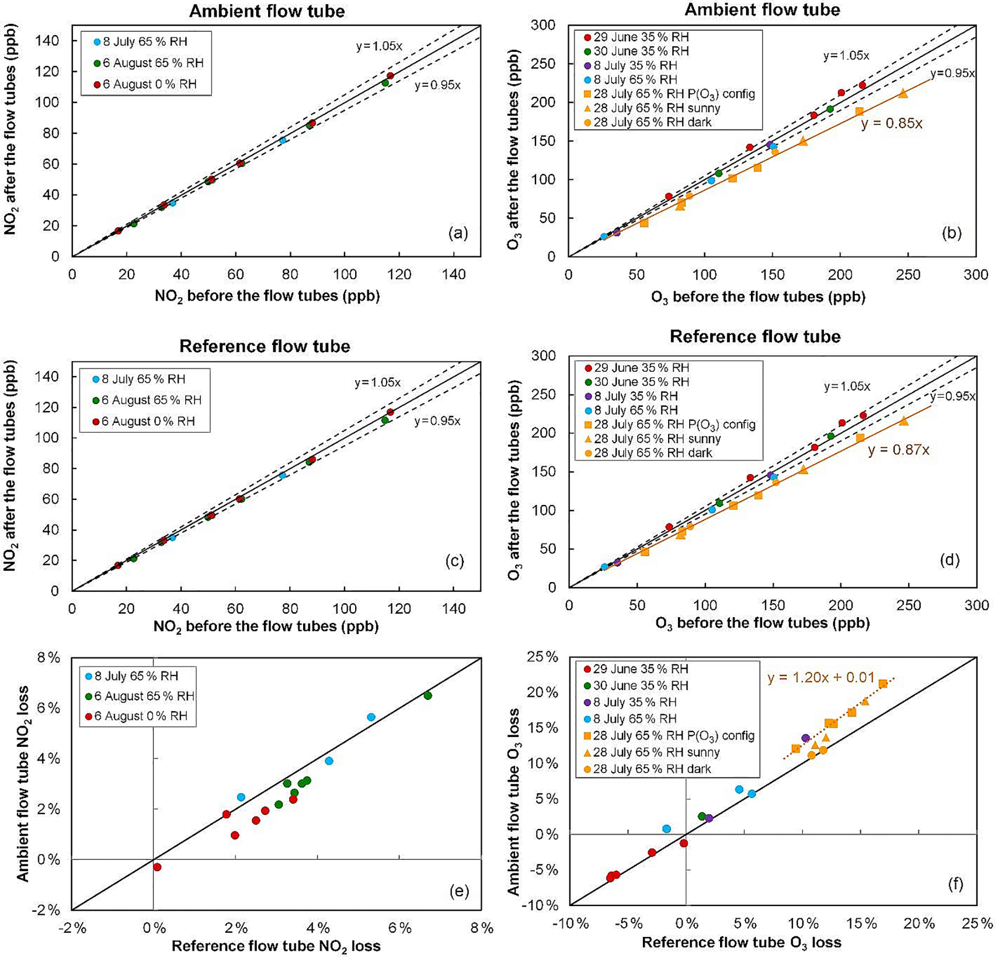
Figure 3 NO₂ and O₃ relative losses measured during the IRRONIC field campaign at different relative humidity values. Losses in the ambient and reference flow tubes are shown in the top and middle panels, respectively. The bottom panel reports the difference in relative losses between the two flow tubes. On 28 July O₃ losses were measured under sunny conditions (orange squares: ambient flow irradiated and reference flow tube covered by the UV filter; orange triangles: both flow tubes irradiated) and dark conditions (orange circles: both flow tubes covered by an opaque cover).

Figure 3 shows the results of NO₂ and O₃ loss tests for the two flow tubes, performed at different dates during 1 month of field operation during the IRRONIC campaign and at different relative humidity values. All NO₂ loss tests were performed under dark conditions, i.e., with both flow tubes covered by an opaque cover. Figure 3a, c and e show that the NO₂ loss is lower than 5 % in both flow tubes and is close to 3 % on average. When the two flow tubes are operated under the same conditions, the relative loss in the reference tube seems to be higher than the loss in the ambient tube by only 1 % at most (Fig. 3e). For an ambient NO₂ mixing ratio of 30 ppbv, a difference of 1 % in NO₂ losses between the flow tubes would lead to a 4 ppbv h⁻¹ bias in the P(O_x) measurements.

Cazorla and Brune (2010) reported an uncertainty of ±14 % for the MOPS instrument due to potential differences in relative humidity between the two sampling chambers, which in turn leads to different NO₂ losses. This was mainly due to a higher temperature in the reference chamber, which is covered by the UV filter. However, the fans used on the OPR instrument to drive the flow of ambient air between the UV filter and the flow tube minimize the temperature differences between the two tubes, leading to relative humidity differences lower than 4 %, as observed during the field testing. Figure 3e also shows that a decrease in relative humidity from 65 to 0 % only leads to a small decrease in the NO₂ loss by 1–2 %. A small difference of 4 % in relative humidity between the two flow tubes is therefore not expected to lead to additional errors in the P(O_x) measurements. Further analysis of the impact of NO₂ losses on the P(O_x) measurements is discussed in the modeling results section.

Ozone loss tests were mainly performed under dark conditions during this campaign. On 28 July, however, O₃ losses were measured with (a) the ambient flow tube exposed to the sunlight and the reference tube covered by the UV filter (orange squares), (b) both flow tubes exposed to the sunlight (orange triangles) and (c) both tubes covered by a dark cover (orange circles). For the first days of the campaign (29 June–8 July), a close inspection of the measurement scatter shown in Fig. 3b, d indicates that the relative loss of O₃ is at most close to 5 %. However, ozone loss tests performed on 28 July, after 1 month of operation in the field, revealed an increase in the relative loss of up to 13–15 %.

Particular attention should be paid to the three different tests performed on 28 July regarding the irradiation conditions. When the losses are quantified under dark conditions (orange circles in Fig. 3f), the losses are equal between the two flow tubes and close to 13 %. However, when the ambient flow tube is irradiated and the reference is covered by the UV filter (orange squares), it can be seen that the relative loss in the ambient tube is higher than in the reference by approximately 3 %. Box modeling has shown that the gas-phase photolysis of O₃ in the ambient flow tube could at most account for 0.05 % of this additional ozone loss. Therefore, there seems to be a photo-enhanced ozone loss that takes place when the ambient flow tube is irradiated. For an ambient O₃ level of 50 ppbv, this difference in O₃ losses would lead to a negative P(O_x) bias of approximately 20 ppbv h⁻¹.

Additional tests were performed after the campaign under different conditions of illumination, RH and ozone mixing ratios to thoroughly investigate the loss of ozone on the quartz material. Overall, these tests showed that the dark loss can be reduced below 5 % for several days of ambient measurements if the quartz flow tubes are conditioned with elevated O₃ mixing ratios at high relative humidity. These results indicate that the low value observed for the loss after the conditioning period may be due to (i) a cleanup of the surfaces, removing unsaturated organic species that may be absorbed on the quartz surface; or (ii) a chemical treatment of the surface, deactivating sites where ozone could be lost during ambient measurements. Tests were also performed to investigate the potential photo-enhanced loss of ozone discussed above. These tests were performed by irradiating the two flow tubes with UV lamps (312 and 365 nm), introducing known mixtures of ozone–zero air in the flow tubes and varying humidity and/or light conditions. While a photo-enhanced loss of ozone was not observed in the reference flow tube covered with the UV filter, a significant photo-enhanced loss of up to 7.5 % was observed for the ambient flow tube when the 312 nm lamps were used, with a dependence on light intensity. In contrast, irradiating the ambient flow tube with the 365 nm lamps did not lead to a photo-enhanced loss, indicating that lower wavelengths are inducing the loss process responsible for the photo-enhanced loss. This issue is further discussed in the field deployment Sect. 3.3.

3.1.3 Heterogeneous HONO production in the flow tubes

The formation of HONO in the flow tubes was investigated in the laboratory by sampling humid zero air (25–80 % RH) enriched with NO₂ at various mixing ratios (0–100 ppbv) and by measuring HONO at the exit of the tubes as described above in Sect. 2.2. Both clean and contaminated (used for more than 1 month during the IRRONIC campaign) flow tubes were tested to assess the magnitude of HONO production rates and to examine whether there is a dependence on NO₂ mixing ratios, humidity and irradiation. Mixing ratios of HONO up to 250 and 700 pptv were measured under dark conditions for clean and contaminated flow tubes, respectively. Higher mixing ratios of up to 1.5 ppbv were measured under irradiated conditions in the ambient flow tube (J(NO₂)= 1.4 × 10⁻³ s⁻¹; J(HONO) = 3.1 × 10⁻⁴ s⁻¹).

Dividing the measured mixing ratios of HONO by the residence time in the flow tubes (i.e., 4.5 min), an average production rate can be calculated under dark and irradiated conditions. It is important to note, however, that HONO is also photolyzed at the wavelengths emitted by the lamps (312 and 365 nm) and production rates calculated under irradiated conditions represent lower bounds. It is estimated that, for the J(HONO) value mentioned above and a negligible loss of HONO from OH + HONO, the HONO production rate will be underestimated by less than 8 %. The dark HONO production is on the order of 9 ppbv h⁻¹ in both flow tubes, while the total HONO production under irradiated conditions (dark + photo-enhanced) can reach up to 20 ppbv h⁻¹ in the ambient flow tube. In the reference flow tube, the UV light did not impact the formation of HONO, since wavelengths below 400 nm are blocked by the UV filter.

The HONO production rate was not observed to depend on NO₂ or humidity and HONO could even be released when no NO₂ was introduced into the contaminated flow tubes. These results strongly suggest that nitro-containing compounds and organic photosensitizers were adsorbed on the walls of the flow tubes and that the HONO production rate depends on contamination levels. Indeed, it was observed that flowing humid zero air in the flow tubes for a few days could reduce the HONO production rate to negligible levels.

3.1.4 Quantification of the conversion efficiency

Based on kinetic considerations for the titration reaction of O₃ by NO, i.e., a rate constant of 1.80 × 10⁻¹⁴ cm³ molecule⁻¹ s⁻¹ at 298 K (Atkinson et al., 2004), a reaction time of 23 s and the addition of 500 ppbv of NO in the conversion unit, an O₃-to-NO₂ conversion efficiency of 99.5 % is expected. These calculations are shown in Fig. 4 (black solid line) for different mixing ratios of NO (50–800 ppbv) together with laboratory measurements (symbols) made at different O₃ levels. This figure shows that a plateau of almost 100 % conversion is observed at NO mixing ratios higher than 500 ppbv. These experimental results are in good agreement with the calculated curve, although the measurements performed at a low O₃ mixing ratio of 3.5 ppbv slightly underpredict the curve for NO mixing ratios lower than 500 ppbv. However, the conversion plateau is reached for all O_x levels and both conversion units (one for each flow tube) for NO mixing ratios higher than 500 ppbv. During the field deployment of the instrument, an NO mixing ratio of 650 ppbv was used to ensure that the difference in conversion efficiency between the two mixing chambers was lower than 0.1 % and could be assumed to be 100 % for both chambers.

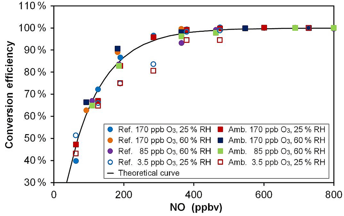
Figure 4 O₃-to-NO₂ conversion efficiency for various NO mixing ratios, O_x levels and relative humidity values. The black curve was calculated from the reaction rate constant between O₃ and NO and a reaction time of 23 s. Open symbols (3.5 ppbv O₃) are hidden behind the plain symbols for NO > 500 ppbv. “Ref.” and “Amb.” refer to the conversion units coupled to the reference and ambient flow tubes, respectively.

In the first version of MOPS (Cazorla and Brune, 2010) the NO₂-to-O₃ conversion was performed by photolyzing NO₂ using a light-emitting diode, achieving a maximum conversion efficiency of 88 % at 17 ppbv of NO₂. In the most recent version of the instrument (Baier et al., 2015), the conversion efficiency was increased to 88–97 % for NO₂ mixing ratios lower than 35 ppbv using a highly efficient UV lamp that provided 10 times more photons than the light-emitting diodes. In the MOPS instrument, however, the conversion efficiency depends on NO₂ levels, as well as on the intensity of the lamp that could drift during a long period of use in the field. In the OPR instrument, the conversion efficiency is stable and does not depend on O₃ mixing ratios. On the other hand, an NO cylinder is required to perform the conversion and possible NO₂ impurities in the cylinder have to be monitored. Indeed, NO₂ impurities coming either from the NO mixture or from NO oxidation in the lines were observed but were kept at low levels of approximately 6–10 ppbv. Since this impurity is present in both the ambient and reference channel, it does not affect the P(O_x) determination.

3.1.5 Detection limit of the OPR

The detection limit (DL) of the CAPS monitor was quantified by sampling zero air for several hours after several days of conditioning with ambient air. The time resolution was set to 1 s and the zero measurements were averaged over 45 s segments, corresponding to the OPR measurement averaging time. The detection limit (3σ) for a 45 s integration time was quantified at 34 pptv. This detection limit for NO₂ together with a residence time of 4.5 min in the flow tubes should lead to a detection limit of 0.6 ppbv h⁻¹ for 2 min P(O_x) measurements (1 min measurement from each flow tube). However, nighttime measurements made during the IRRONIC field campaign revealed that the measurement scattering for the complete setup (flow tubes + O₃-to-NO₂ conversion unit + CAPS) was significantly larger than that expected from the noise of the CAPS monitor. Based on the observed nighttime 1σ variability of 2.1 ppbv h⁻¹, a limit of detection (3σ) of 6.2 ppbv h⁻¹ was inferred for the OPR instrument. The scatter in P(O_x) measurements does not only depend on the precision of the CAPS monitor, but also depends on how fast each flow tube responds to variations in O_x at the inlet. Indeed, if the time constant for the response is slightly different between the two flow tubes, fluctuations of O_x species at the inlet will introduce some scatter in the OPR measurements. In addition, small changes in temperature and humidity may evenly affect O_x losses in each flow tube, leading to additional scatter in the P(O_x) measurements.

3.2 Numerical modeling

As mentioned in the experimental section, several days from different field campaigns were selected to model ambient P(O_x), P(O_x) in both flow tubes and the impact of some operating conditions on the OPR measurements. The results from 30 May 2010 of the CalNex field campaign were selected to illustrate the discussion, and results from the other days are shown in the Supplement (Figs. S4, S5, S7–S9). A detailed analysis of the chemistry occurring in each flow tube is discussed below to assess the reliability of OPR measurements.

Figure 5 OH (a, b) and total peroxy (HO₂+RO₂; c, d) radical budgets for 30 May 2010 of the CalNex 2010 campaign. Radical budgets modeled for the ambient (a, c) and the reference (b, d) flow tubes. The OH chain length is also presented in an insert (a, b) for each flow tube. “Init” in the legend indicates initiation reactions and “hv” represents photons.

3.2.1 Radical budget in flow tubes

An analysis of the radical budget was performed in each flow tube to gain insights into the processes driving radical production and loss routes. Figure 5 shows the production and loss rates of OH (upper panel) and peroxy radicals (lower panel) for each flow tube on 30 May 2010 during CalNex. The production and loss rates were calculated taking into account initiation, propagation and termination processes as described below.

OH production rates were calculated from photolytic reactions involving closed shell molecules (O₃, HONO, H₂O₂, HNO₃, HO₂NO₂ and organic peroxides), reactions of O₃ with alkenes and the propagation of HO₂ by reaction with NO. Loss routes of OH include propagation reactions to HO₂ and RO₂ by reaction with CO and VOCs and termination reactions of OH with NO₂ and other species (NO, PANs, HNO₃, HONO and HNO₄). For peroxy radicals, production routes include the photolysis of organic species (carbonyls, organic peroxides and organic nitrates), the ozonolysis of alkenes, PAN decomposition and the propagation of OH. Loss routes were calculated from reactions of peroxy radicals with NO_x, self or cross reactions between peroxy radicals, and propagation of HO₂ to OH.

Figure 5 clearly shows that the UV filter covering the reference flow tube leads to a decrease in the initiation rates of all radicals by more than a factor of 10 and a decrease in their propagation rates by at least a factor of 30. In the ambient flow tube, photolytic reactions of oxygenated VOCs are the most important initiation routes of peroxy radicals, with a contribution of approximately 95 %. HONO and O₃ photolysis are the most important initiation routes of OH, contributing approximately 45 % each. In the reference flow tube, the primary route of radical initiation is O₃–alkenes reactions since wavelengths below 400 nm are suppressed.

The propagation reactions are important in both flow tubes for the production and loss of OH and peroxy radicals. However, the partitioning between initiation and propagation processes is different in the two tubes, which in turn leads to different OH chain lengths. The OH chain length is calculated as the rate of propagation of HO₂ to OH divided by the total initiation of RO_x radicals. As can be seen from Fig. 5, the OH chain length is fairly constant at a value of 3 in the ambient flow tube, while in the reference flow tube it quickly decreases to unity for most of the day and to values lower than unity in the late afternoon. Therefore, in addition to lowering initiation rates of radicals, the UV filter allows the reduction of ozone production by lowering the cycling efficiency within the pool of RO_x radicals.

A close inspection of the radical termination rates in Fig. 5 indicates that the peroxy–NO_x termination reactions are almost suppressed in the reference flow tube. This observation is also supported by Fig. S6, which shows time series of the peroxy radicals (HO₂ and RO₂) and NO in each flow tube at a residence time of 4.5 min. Since NO₂ photolysis is almost eliminated in this tube, the O₃–NO_x PSS is shifted towards NO₂ due to the reaction of NO with O₃. As a result, NO mixing ratios in the reference flow tube are at least 1 order of magnitude lower than in the ambient flow tube. The propagation rate from HO₂+ NO is therefore reduced and the OH + NO₂ loss route is enhanced, leading to the shorter OH chain length discussed above. It is also interesting to note that peroxy radical mixing ratios in the reference flow tube are of the same order of magnitude as in the ambient flow tube. This counterintuitive observation is also due to the consumption of NO in the reference flow tube that leads to a longer lifetime for the peroxy radicals, as shown in Fig. S6.

Calculating P(O_x) from Eqs. (1) to (3) results in ozone production rates in the ambient flow tube, P(O_x)_amb, in good agreement with the modeled P(O_x)_atm values, as shown in Fig. 6, with a small underestimation of approximately 10 % on average. However, significant ozone production rates are also observed in the reference flow tube, which can reach up to 4 ppbv h⁻¹ on this day, while higher values were observed on other days (e.g., 30 ppbv h⁻¹ on 21 March 2006 of the MCMA 2006 campaign, Fig. S10). Ozone production rates in the reference flow tube are about 10–15 % of that observed in the ambient flow tube for most of the day. It is important to note, however, that this ozone production is in reality O_x (= O₃+ NO₂) production, since NO₂ photolysis is almost suppressed in the reference flow tube. These results indicate that the assumptions initially made on the principle for P(O_x) measurements, i.e that P(O_x) in the ambient flow tube mimics P(O_x) in the atmosphere and P(O_x) in the reference flow tube is not significant, are not completely fulfilled. Based on the modeling results discussed above, the accuracy of the measurements could be significantly impacted by O_x production in the reference flow tube.

Figure 6 Modeling comparison of P(O_x) values. (a) Ozone production rates modeled for the atmosphere, P(O_x)_atm; the ambient flow tube, P(O_x)_amb; and the reference flow tube, P(O_x)_ref, for 30 May 2010 of the CalNex 2010 campaign. (b) Comparison of modeled ozone production rates for the OPR, P(O_x)_OPR, and the atmosphere, P(O_x)_atm, for 30 May 2010. Inserts: correlations between P(O_x)_atm and P(O_x)_amb (a) as well as between P(O_x)_atm and P(O_x)_OPR (b), color-coded by the time of day.

P(O_x)_OPR was calculated from Eq. (6), using an O₃-to-NO₂ conversion efficiency of 100 %, and is also shown in Fig. 6. As discussed above, P(O_x)_OPR underestimates the modeled P(O_x)_atm, mainly due to significant O_x production in the reference flow tube. The scatterplot shown as insert in this figure indicates that a negative bias of approximately 20 % would be observed for P(O_x) measurements performed on this day. A negative bias ranging from 15 to 20 % was observed during the other 3 days that were modeled (Fig. S11).

As mentioned in the experimental section, concentrations of peroxy radicals obtained as model outputs from the modeling of P(O_x)_atm were constrained for the simulations inside the flow tubes, assuming that most of these species are not lost if a short high-flow rate sampling inlet is used. However, simulations were also performed without constraining the peroxy radicals to assess the impact on the simulation results. These simulations have shown that P(O_x) values are lower by 10 and 30 % in the ambient and reference flow tubes, respectively, when peroxy radicals are not constrained. Overall, the measured ozone production, which is the difference between P(O_x) in the two flow tubes, would only decrease by 2–4 %. Therefore, not constraining peroxy radicals in the simulations does not impact the comparison between P(O_x)_atm and P(O_x)_OPR, with P(O_x)_OPR underestimating P(O_x)_atm by 15–20 %.

However, the reason for this disagreement depends on whether peroxy radicals are constrained. When peroxy radicals are constrained, the disagreement is mainly caused by O_x production in the reference flow tube. In contrast, when peroxy radicals are not constrained, this disagreement is due to an underestimation of P(O_x)_atm by P(O_x)_amb. This underestimation is the result of a latency in the first part of the ambient flow tube due to the time needed to reproduce the radicals, which is on the order of 1–2 min. It is very likely that only a fraction of the peroxy radicals will be transferred to the flow tubes and a combination of the two issues discussed above will lead to the negative bias of 15–20 %.

Figure 7 Sensitivity tests performed for 30 May 2010 (CalNex 2010) to assess the impact on the P(O_x) measurements of the (a) O₃-to-NO₂ conversion efficiency, (b) NO₂ and (c) O₃ dark losses, (d) heterogeneous HONO formation, (e) dilution of ambient air and (f) NO₂ loss towards HONO production in the flow tubes. The results presented here correspond to the 2 h of the day identified as lower (blue squares) and upper (orange squares) limits of the impact on the P(O_x) measurements. The daily average behavior is also shown using green triangles.

3.2.2 Sensitivity tests – assessment of the impact of operating conditions on OPR measurements

Figure 7 shows the dependence of P(O_x)_OPR on the O₃-to-NO₂ conversion efficiency, O₃ and NO₂ surface losses, surface production of HONO and a dilution of the sampled air. The results are displayed for two different times of the day, characterized by different O₃ and NO₂ mixing ratios, which have been identified as upper (orange squares) and lower (blue squares) limits for the impact on the P(O_x) measurements. In addition, these results are also displayed using daily averaged values (green triangles), which are more representative of the average impact of a particular parameter on P(O_x) measurements. The figures described below are for the CalNex campaign during 30 May 2010. Results from the other days are shown in the Supplement (Figs. S12–S14).

Figure 7a shows that P(O_x)_OPR is very sensitive to the O₃-to-NO₂ conversion efficiency. For instance, a conversion efficiency of 85 % would lead to an underestimation of the P(O_x) measurements by 20–60 % (≈ 35 % on average), depending on the chemical composition of the air mass. It is interesting to see that the change in P(O_x)_OPR, expressed as the ratio between P(O_x)_OPR at a conversion efficiency lower than 100 % and P(O_x)_OPR at a conversion efficiency of 100 % (base simulation), changes linearly with the conversion efficiency. The slope of the straight line can be used as an indicator to gauge the impact of the conversion efficiency on P(O_x) measurements throughout the day. As can be seen from Eq. (6), for the limiting case of C= 0, the measured P(O_x) is determined by the absolute NO₂ difference between the two flow tubes. The O₃–NO_x PSS is shifted towards NO₂ in the reference flow tube, due to the lack of NO₂ photolysis, reducing the NO₂ difference between the two tubes and lowering the measured P(O_x). These results stress the need to reach a conversion efficiency better than 98 % to keep this artifact below 5 %. The OPR instrument described in this study exhibits a conversion efficiency higher than 99.9 % and is not impacted by this issue.

Relative surface losses of 3 and 5 % have been observed for NO₂ and O₃, respectively, during the laboratory and field testing (Sect. 3.1.2). Figure 7b shows that a relative NO₂ loss of 3 % in the flow tubes can lead to an overestimation of up to 8 % (≈ 3 % on average). On the other hand, Fig. 7c shows that a 5 % relative loss of O₃ can lead to an underestimation of up to 30 % (≈ 5 % on average). These contrasting effects can be explained as follows: ozone in the reference flow tube is lower than in the ambient flow tube, due to the conjunction of a lower production rate of ozone and a shift of the O₃–NO_x PSS towards NO₂. A similar relative loss of ozone in the two flow tubes will therefore lead to a larger absolute loss of O_x species in the ambient flow tube, which in turn will lead to an underestimation of the P(O_x) measurements (Eq. 6). In contrast, NO₂ is higher in the reference flow tube and a loss of NO₂ will lead to a larger absolute loss of O_x species in the reference flow tube and, as a consequence, to an overestimation of the P(O_x) measurements.

Table 1 Sources of errors on P(O_x) measurement. Upper limits and campaign averages of errors assessed from modeling the selected days of the MCMA 2006 and CalNex 2010 field campaigns (see text). FT: flow tube.

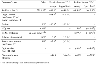
^a From laboratory testing; ^b from model simulations; ^c from estimation.

Figure 8 Time series of selected trace gases, J(NO₂), measured ΔO_x and ΔP(O_x) values during 4 days of the IRRONIC campaign when 6 ppbv of NO was intermittently added in the flow tubes. The light colors on ΔO_x correspond to 2 min measurements while the darker colors are 20 min averaged values. Error bars on ΔP(O_x) are 1σ on the averaged 20 min measurements.

Figure 7d shows how a heterogeneous production of HONO can impact the P(O_x) measurements. In these simulations, a HONO source was added in the model, with a production rate of 10 ppbv h⁻¹ in both flow tubes (dark HONO production) and an additional varying production rate in the ambient flow tube (enhanced HONO production). The x axis presents the HONO production rate in the ambient flow tube, where 10 ppbv h⁻¹ corresponds to the dark production only. Moreover, this figure indicates that HONO production rates of 20 ppbv h⁻¹ in the ambient flow tube, similar to experimental observations, can lead to an overestimation of the P(O_x) measurements by up to 40 % (≈ 27 % on average). This overestimation results from HONO photolysis in the ambient tube, which leads to additional OH production, which in turn leads to an enhancement of VOC-oxidation rates and ozone production. Additional simulations were also performed assuming that NO₂ molecules lost on the surface were equally converted into HONO in both flow tubes (Fig. 7f), although it is unlikely that the conversion yield of NO₂ into HONO is 100 %. The results indicate that, for a relative NO₂ loss of 3 %, P(O_x) could be overestimated by up to 15 % (10 % on average). Note that the impact of this HONO formation adds up to the previously discussed overestimation due to the NO₂ loss.

Figure 7e displays how the injection of zero air at the periphery on the PTFE inlets impacts P(O_x) measurement through a dilution of the sampled air. As can be seen from this figure, a 10 % dilution leads to a less than 9 % underestimation of P(O_x).

Additional sensitivity tests (not shown) were performed to test the impact of a temperature increase in the reference flow tube due to heat release by the UV filter, as well as reactions of OH with NO_z species that produce NO₂. A temperature increase of 5 % in the reference flow tube (1 ^∘C increase at 20 ^∘C) can lead to an underestimation of up to 5 %, while the O_x production from reactions of OH with NO_z species can lead to an overestimation of up to 3 %.

3.2.3 Conclusions on potential biases on P(O_x)_OPR measurements

From the above discussion, we can conclude that there are two main sources of errors. The first source of errors is due to O_x production in the reference flow tube and the latency for RO_x reformation in the ambient flow tube, with the extent of each depending on the fraction of ambient peroxy radicals that is transmitted into the flow tubes. The combination of these two issues can lead to an underestimation of ambient P(O_x) by 15–20 % on average for the conditions observed during the MCMA 2006 and CalNex 2010 campaigns. The second main source of errors is caused by a surface production of HONO in the ambient flow tube. Based on a HONO production rate of 20 ppbv h⁻¹, P(O_x) would be overestimated by approximately 30 % on average. Additional sources of errors are due to the 4.9 % uncertainty on the flow tube residence time, 5 % O₃ and 3 % NO₂ surface losses, the dilution by 10 % of the sampled air, a possible temperature increase of 5 % in the reference flow tube and O_x production from reactions of OH with NO_z species. Daily averaged values and upper bounds of errors associated with these factors, as derived from all modeled days, are reported in Table 1.

Based on the daily average values reported in Table 1, direct sums of the potential negative and positive biases lead to −44 and +40 %, respectively. However, the magnitude of each error will depend on the atmospheric composition and positive errors will, to some extent, cancel out with negative errors. A quadratic sum of all these potential errors leads to a range of ±36 %. The estimation of these errors is based on ambient conditions observed in two different environments, with different air compositions for 4 different days. It is safe to assume that similar error values would be observed in other urban environments.

3.3 Current limitations for field operation

As mentioned in Sect. 2.4, OPR measurements were performed during the IRRONIC field campaign. Figure 8 displays time series for a subset of measurements performed from 10 to 14 July 2015, including two anthropogenic VOCs (toluene and acetylene), a biogenic VOC (isoprene) and inorganic species (O₃, NO and NO₂). It is clear from this figure that the measurement site was mainly impacted by biogenic emissions, with isoprene reaching at least 5 ppbv most of the days, while anthropogenic VOCs were low (< 500 pptv). In addition, NO_x levels were lower than 3 ppbv on these days, confirming the low impact of anthropogenic emissions. These observations indicate that the photochemistry was mainly driven by the oxidation of biogenic VOCs under low NO_x conditions, similar to those observed in other forested areas (Griffith et al., 2013). Isoprene is very reactive with the hydroxyl radical and the strong diurnal variation in this species led to a large range of OH reactivity (from a few s⁻¹ up to 30 s⁻¹, not shown). The conjunction of the latter with low levels of NO_x makes this a site of particular interest to study the sensitivity of ozone formation to NO_x by adding NO_x in the OPR instrument as described in the experimental Sect. 2.4.

Due to the low levels of ambient NO_x, ozone production rates at the site were lower than the OPR detection limit of 6.2 ppbv h⁻¹ (Sect. 3.1.5). Indeed, P(O_x) calculations based on total peroxy radical measurements performed using the peroxy radical chemical amplifier technique indicated peak ozone production rates of approximately 2 ppbv h⁻¹ (not shown). Ambient measurements performed by the OPR instrument without addition of NO should therefore be scattered around zero within the measurement precision. Figure 8 also displays ΔO_x values (difference in O_x mixing ratios between the two flow tubes) measured by the instrument without the addition of NO (ΔO${}_x^{\mathrm{zero}}$, blue diamonds). While ΔO${}_x^{\mathrm{zero}}$ was scattered around zero during nighttime, it consistently exhibited large negative values during daytime (−1 to −5 ppbv), indicating that O_x mixing ratios in the ambient flow tube were lower than in the reference flow tube.

It is interesting to note that ΔO${}_x^{\mathrm{zero}}$ values are anticorrelated with J(NO₂) (Fig. 8). Covering the ambient flow tube with a similar UV filter than the reference flow tube, i.e., operating the two tubes under similar irradiation, showed that ΔO_x increases towards less negative values and ultimately reaches zero. This behavior indicates that the higher loss rate of O_x species in the ambient flow tube is due to the solar irradiation and points towards a photo-enhanced surface loss of O_x species initiated by photons at wavelengths lower than 400 nm. As ambient NO₂ mixing ratios were much lower than the observed loss of O_x, this photo-enhanced loss involves a loss of ozone. For an ambient O₃ level of 40 ppbv, as usually observed during the field measurements, a ΔO${}_x^{\mathrm{zero}}$ of −3 ppbv corresponds to a 7.5 % difference in O₃ losses between the two flow tubes and an ozone loss rate higher by approximately 39 ppbv h⁻¹ in the ambient flow tube compared to the reference flow tube. This issue was further investigated in the laboratory. As mentioned in Sect. 3.1.2, tests performed using artificial irradiation and mixtures of humid air and ozone confirmed that light-induced processes at wavelengths lower than 400 nm lead to a loss of ozone at the surface of the ambient flow tube. It was found that this loss depends on ambient ozone levels, J values and absolute humidity.

This version of the OPR instrument is therefore not suitable to perform ambient P(O_x) measurements since the measured ΔO_x is a combination of ambient ozone production and surface-O₃ losses in the ambient flow tube. For this reason, the OPR measurements were focused on investigating the sensitivity of P(O_x) to NO_x, by recording the relative change in P(O_x) when the chemical composition of ambient air was perturbed by an addition of NO. For these measurements, it is assumed that ΔO${}_x^{\mathrm{zero}}$ is representative of the instrumental zero and ΔO${}_x^{\mathrm{zero}}$ measurements are referred to as the “baseline” in the following. ΔO_x measurements performed with an addition of NO are assumed to deviate from ΔO${}_x^{\mathrm{zero}}$ due to a change in ozone production in the ambient flow tube, while the surface loss of ozone is assumed to be unchanged. This measurement step is denoted ΔO${}_x^{\mathrm{NO}}$. The difference between ΔO${}_x^{\mathrm{zero}}$ and ΔO${}_x^{\mathrm{NO}}$ divided by the residence time in the flow tubes therefore provides a quantification of the change in P(O_x), referred to as ΔP(O_x), due to the addition of NO. The validity of the assumption that the O₃ photo-enhanced surface loss is not disturbed by the addition of NO is discussed below.

Investigating the ozone production sensitivity to NO is outside the scope of this paper and we only present measurements performed when 6 ppbv of NO was added in the instrument to illustrate its current performances and limitations. Figure 8 displays time series of ΔO${}_x^{\mathrm{NO}}$ (orange diamonds) when 6 ppbv of NO was added in the flow tubes. When NO is added, there is almost no change in ΔO_x during nighttime. In the absence of sunlight, NO only converts O₃ into NO₂ and the amount of O_x measured by the CAPS monitor does not change. During daytime, ΔO${}_x^{\mathrm{NO}}$ is higher than ΔO${}_x^{\mathrm{zero}}$, suggesting production of ozone in the ambient flow tube. The difference between ΔO${}_x^{\mathrm{NO}}$ and ΔO${}_x^{\mathrm{zero}}$, divided by the residence time in the flow tubes, represents the change in ozone production rates and is displayed in the bottom panel of Fig. 8 as ΔP(O_x). Changes in ozone production of up to 20 ppbv h⁻¹, well correlated with J(NO₂), are observed for these days. With ozone production being NO_x limited in this environment, a positive change in P(O_x) is indeed expected when a small amount of NO_x is added to the flow tubes.

However, the assumption that the photo-enhanced surface loss of ozone does not change when NO is added may breakdown for large NO mixing ratios. Indeed, the addition of NO in the flow tubes leads to the conversion of a significant fraction of O₃ into NO₂, which in turn reduces the absolute loss of O₃ in the ambient flow tube, leading to a shift of the ΔO${}_x^{\mathrm{zero}}$ baseline to less negative values. ΔP(O_x) values reported in Fig. 8 will therefore be the combination of a change in ozone production and a change in the absolute loss of O₃. If the change in the ozone loss rate is significant compared to the change in the ozone production rate, this could lead to an overestimation of the change in ozone production. An assessment of this measurement bias requires modeling the chemistry in both flow tubes to separate the two contributions, i.e the changes in (i) ozone production and in (ii) ozone loss. While this work is outside the scope of this publication, which focuses on the performances and limitations of the OPR instrument, it is interesting to note that preliminary modeling indicates a bias lower than 5 pbbv h⁻¹ when 6 ppbv of NO is added.

The field deployment during IRRONIC revealed an additional bias in P(O_x) measurements due to a photo-enhanced loss of ozone at the inner surface of the ambient flow tube and the difficulty in probing changes in P(O_x) when the sampled air mass is perturbed by an addition of NO. Ambient measurements of P(O_x) with the current version of the OPR would necessitate performing frequent zeros of the instrument to track the ozone loss, and unfortunately a simple solution to do so was not found. This work shows that the sampling part of the OPR instrument needs to be rethought to remove (or reduce to a negligible level) the photo-enhanced surface loss of ozone, which is a prerequisite to acquiring an instrument capable of reliable measurements of ozone production rates.

3.4 Comparison to previously published instruments and potential improvements for the OPR instrument

Previous studies (Cazorla and Brune, 2010; Baier et al., 2015) have shown that measurements of ambient ozone production rates are feasible. Baier et al. (2015) reported that the zero of their MOPS instrument was achieved by removing the UV filter from the reference chamber for a full day to record a diurnal profile of ΔO_x, which was then subtracted from the raw ΔO_x measurements on other days. This zeroing procedure was also tested on the OPR instrument, but led to unrealistically high ambient P(O_x) values of approximately 40 ppbv h⁻¹ for the low-NO_x forested environment of IRRONIC. This result also suggests that altering the irradiation conditions of the OPR flow tubes leads to a wrong zero of the instrument. This zeroing technique seems to provide better results for the MOPS instrument and it is possible that the design used for the MOPS sampling chambers or the material used to build them (FEP) make it less sensitive to light-dependent surface reactions.

The instrument design reported by Sadanaga et al. (2017) does not seem to be significantly impacted by a photolytic loss of ozone on the quartz flow tubes whose inner surface was coated with Teflon^®. Interestingly, these authors report dark losses of ozone on the order of 8–10 % on the uncoated quartz surface for a residence time of 21 min in the tubes, which are consistent with the reported dark loss of less than 5 % observed in our study for O₃-conditioned flow tubes and a residence time of 4.5 min. The Teflon^® coating seems to remove or to reduce the photolytic loss of ozone to a negligible level on this instrument.

Since the main artifacts on the OPR instrument are caused by heterogeneous surface reactions in the flow tubes, i.e., HONO production (Sect. 3.2.2) and ozone losses (Sect. 3.2.2 and 3.3), the flow tubes should be redesigned to reduce the impact of physicochemical processes occurring near the quartz surface on the ozone production chemistry occurring at the center of the tubes. A solution worth investigating would be to minimize surface reactions by coating the inner surface of the flow tubes with Teflon^® as in Sadanaga et al. (2017) or by applying a chemical treatment on the quartz surface, which should help in removing reactive sites. The latter has already been applied for laboratory kinetic experiments to clean reactor surfaces. Interestingly, it was reported that this type of treatment can also reduce HONO production on quartz surfaces (Laufs and Kleffmann, 2016).

Other potential solutions would be to (i) increase the diameter of the tubes to reduce the surface-to-volume ratio and (ii) shorten their lengths together with an increase in the total flow rate to reduce the contact time between trace gases and the walls. A shorter residence time would also lead to a shorter air-exchange time, which in turn would help in minimizing the scatter in ΔO_x measurements and would help improve the time resolution necessary to generate independent P(O_x) measurements. However, a shorter residence time would also lead to a lower detection limit and a tradeoff between these two parameters will likely have to be made.

Regarding the deployment of these OPR instruments in the field, a reliable zeroing method would be suitable for both ambient P(O_x) and P(O_x) sensitivity measurements. An interesting solution would be to introduce a radical scavenger in the flow tubes to suppress ozone production, but a suitable compound has yet to be identified.

4 Conclusions

An instrument dedicated to direct measurements of ozone production rates was developed and consists of two quartz flow tubes, an O₃-to-NO₂ conversion unit and an Aerodyne CAPS NO₂ monitor. This setup, compared to the NO₂-to-O₃ conversion approach previously published in the literature, presents the advantage of a conversion efficiency higher than 99.9 %, which is independent of ambient O_x levels. Laboratory and field testing performed to characterize the performance of this instrument showed that dark losses of O₃ and NO₂ inside the flow tubes are lower than 5 and 3 %, respectively. However, it was shown that dark ozone losses can increase after a long exposure of the flow tubes in the field and frequent reconditioning steps should be performed during nighttime by flowing humid air and O₃ through the tubes to keep the loss below 5 %.

A modeling exercise taking advantage of measurements from previous urban field campaigns showed that a latency in ozone production in the ambient flow tube and a net ozone production in the reference flow tube can lead to an 18 % measurement underestimation of ambient P(O_x) on a daily average for the conditions of the MCMA 2006 and CalNex 2010 field campaigns. However, the magnitude of this underestimation depends on the chemical composition of ambient air, and it is recommended to assess this potential bias for future campaigns.

Sensitivity tests performed during the modeling exercise highlighted the importance of a high conversion efficiency, since a conversion of 95 %, which is only 5 % lower than the maximum, could lead to an underestimation of ambient P(O_x) by approximately 20 % on a daily average for the two selected field campaigns. A dark surface loss of ozone in the flow tubes would lead to an underestimation of ambient P(O_x), while an NO₂ loss would lead to an overestimation. On a daily average, an underestimation of 10 % and an overestimation of 5 % were assessed for an O₃ loss of 5 % and an NO₂ loss of 2 %, respectively. A photo-enhanced production of HONO in the ambient flow tube on the order of 20 ppbv h⁻¹ would also lead to an overestimation of ambient P(O_x) by 27 % on a daily average. Overall, a quadratic sum of these potential biases for the conditions of the two urban field campaigns leads to a range of errors of ±37 % on a daily average.

As shown from the first deployment of the OPR instrument, there is an additional bias due to a photo-enhanced loss of O₃ taking place in the ambient flow tube. This requires improving the sampling design to be able to perform reliable ambient measurements. The first field deployment of the OPR instrument was performed in a low NO_x environment, allowing the focusing of the study on the sensitivity of ozone production to NO_x. Significant changes in ozone production rates were observed (up to 20 ppbv h⁻¹) when 6 ppbv of NO_x was added in the flow tubes, consistent with an NO_x-limited production regime.