the Creative Commons Attribution 4.0 License.
the Creative Commons Attribution 4.0 License.
 | 18 Feb 2019
Polarization lidar: an extended three-signal calibration approach
Cristofer Jimenez
Albert Ansmann
Ronny Engelmann
Moritz Haarig
Jörg Schmidt
Ulla Wandinger
We present a new formalism to calibrate a three-signal polarization lidar and to measure highly accurate height profiles of the volume linear depolarization ratios under realistic experimental conditions. The methodology considers elliptically polarized laser light, angular misalignment of the receiver unit with respect to the main polarization plane of the laser pulses, and cross talk among the receiver channels. A case study of a liquid-water cloud observation demonstrates the potential of the new technique. Long-term observations of the calibration parameters corroborate the robustness of the method and the long-term stability of the three-signal polarization lidar. A comparison with a second polarization lidar shows excellent agreement regarding the derived volume linear polarization ratios in different scenarios: a biomass burning smoke event throughout the troposphere and the lower stratosphere up to 16 km in height, a dust case, and also a cirrus cloud case.
- Article
(3727 KB) - Full-text XML
- BibTeX
- EndNote


Atmospheric aerosol particles influence the evolution of clouds and the formation of precipitation in complex and not well-understood ways. Strong efforts are needed to improve our knowledge about aerosol–cloud interaction and the parameterization of cloud processes in atmospheric (weather and climate) models and weather forecasts and especially to decrease the large uncertainties in future climate predictions (IPCC, 2014; Huang et al., 2007; Fan et al., 2016). In addition to more measurements in contrasting environments with different climatic and air pollution conditions, new experimental (profiling) methods need to be developed to allow an improved and more direct observation of the impact of different aerosol types and mixtures on the evolution of liquid-water, mixed-phase, and ice clouds occurring in the height range from the upper planetary boundary layer to the tropopause. Active remote sensing is a powerful technique to continuously and coherently monitor the evolution and life cycle of clouds in their natural environment.
Recently, Schmidt et al. (2013a, b, 2015) introduced the so-called dual-field-of-view (dual-FOV) Raman lidar technique, which allows us to measure aerosol particle extinction coefficients (used as aerosol proxy) close to cloud base of a liquid-water cloud layer and to retrieve, at the same time, cloud microphysical properties such as cloud droplet effective radius and cloud droplet number concentration (CDNC) in the lower part of the cloud layer. In this way, the most direct impact of aerosol particles on cloud microphysical properties could be determined. However, the method is only applicable after sunset (during nighttime) and signal averaging of the order of 10–30 min is required to reduce the impact of signal noise on the observations to a tolerable level. As a consequence, cloud properties cannot be resolved on scales of 100–200 m horizontal resolution or 10–30 s. To improve the dual-FOV measurement concept towards daytime observations and shorter signal averaging times (towards timescales allowing us to resolve individual, single updrafts and downdrafts) we developed the so-called dual-FOV polarization lidar method (Jimenez et al., 2017, 2018). This technique makes use of strong depolarization of transmitted linearly polarized laser pulses in water clouds by multiple scattering of laser photons by water droplets (with typical number concentrations of 100 cm−3). This novel polarization lidar method can be applied to daytime observations with resolutions of 10–30 s. An extended description of the method is in preparation (Jimenez et al., 2019).
Highly accurate observations of the volume linear depolarization ratio are of fundamental importance for a successful retrieval of cloud microphysical properties by means of the new polarization lidar technique. In this article (Part 1 of a series of several papers on the dual-FOV polarization lidar technique), we present and discuss our new polarization lidar setup and how the lidar channels are calibrated. The basic product of a polarization lidar is the volume linear depolarization ratio, defined as the ratio of the cross-polarized to the co-polarized atmospheric backscatter intensity, and is derived from lidar observations of the cross- and co-polarized signal components, or alternatively, from the observation of the cross-polarized and total (cross- + co-polarized) signal components. Cross- and co-polarized denote the plane of linear polarization, orthogonal and parallel to the linear polarization plane of the transmitted laser light, respectively. Reichardt et al. (2003) proposed a robust concept to obtain high-quality depolarization ratio profiles by simultaneously measuring three signal components, namely the cross- and co-polarized signal components and additionally the total elastic backscatter signal. We will follow this idea as described in Sect. 2. Reichardt et al. (2003) assumed that the laser pulses are totally linearly polarized. Recent studies, however, have shown that the transmitted laser pulses can be slightly elliptically polarized (David et al., 2012; Freudenthaler, 2016; Bravo-Aranda et al., 2016; Belegante et al., 2018). We will consider this effect in our extended approach of the three-channel depolarization technique. We further extend the formalism by considering realistic strengths of cross talk among the three channels and we propose a practical inversion scheme based on the determination of the instrumental constants for the retrieval of high-temporal-resolution volume depolarization ratio profiles.
The article is organized as follows. In Sect. 2, the lidar instrument is described. The new methodology to calibrate the lidar system and to obtain high-quality depolarization ratio observations is outlined in Sect. 3. Section 4 presents and discusses atmospheric measurements performed to check and test the applicability of the new methodology. Concluding remarks are given in Sect. 5.
A sketch of the instrumental setup, providing an overview of the entire lidar system, is shown in Fig. 1. MARTHA (Multiwavelength Tropospheric Raman lidar for Temperature, Humidity, and Aerosol profiling) has a powerful laser transmitting in total 1 J per pulse at a repetition rate of 30 Hz and has an 80 cm telescope. It is thus well designed for tropospheric and stratospheric aerosol observations (Mattis et al., 2004, 2008, 2010; Schmidt et al., 2013b, 2014, 2015; Jimenez et al., 2017, 2018). MARTHA belongs to the European Aerosol Research Lidar Network (EARLINET) (Pappalardo et al., 2014). We implemented a new three-signal polarization lidar receiver unit to the left side of the large telescope (see Fig. 1). The new receiver setup is composed of three independent telescopes co-aligned with the lidar transmitter.
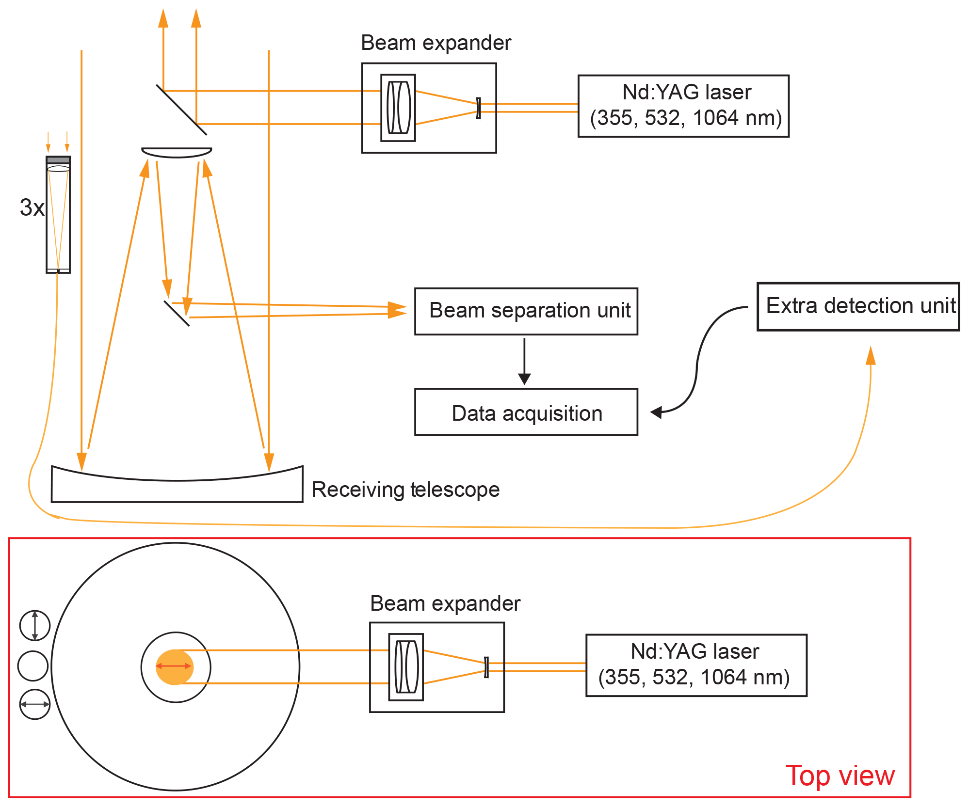
Figure 1Overview of the EARLINET lidar MARTHA. The three-signal receiver unit of the new polarization lidar setup (details are shown in Fig. 2) is integrated into the MARTHA telescope construction (left side in both of the sketches). The outgoing laser beam is 54 cm away from the new polarization-sensitive receiver unit. The main plane of linear polarization of the laser pulses and the polarization sensitivity of cross- and co-polarized receiver channels are indicated by arrows in the top-view sketch.
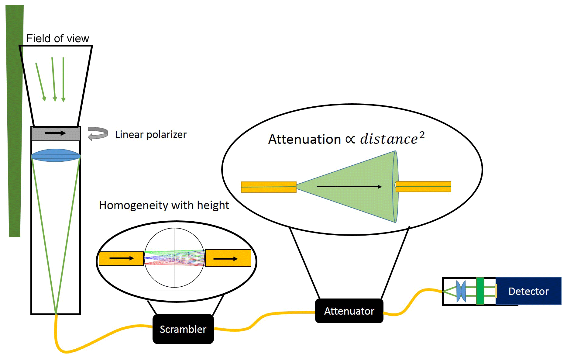
Figure 2Sketch of one of the three identical receiver channels of the three-signal polarization lidar. The different parts are explained in the text.
Figure 2 provides details of the new polarization-sensitive channels. Each of the small receiver telescopes consists of 2 in. (50.8 mm) achromatic lens with a focal length of 250 mm. An optical fiber with an aperture of 400 µm is placed at the focal point of the lens. The resulting FOV is 1.6 mrad. The receivers have in principle the same overlap function since they are identical and are implemented into the large telescope at the same distance from the laser beam axis. The laser-beam receiver-FOV overlap (obtained theoretically) is complete at about 650 m above the lidar (Stelmaszczyk et al., 2005).
A 2 mm ball lens is placed at the output of the fiber (scrambler in Fig. 2) in order to remove the small sensitivity of the interference filter to the changing incidence angle of backscattered light in the near-range. A spatial attenuation unit which consists of two optical fibers is integrated in the receiver setup, replacing the usual setup with neutral density filters. The distance between the two fibers with a given aperture and thus the strength of the incoming lidar return signal can be changed. The attenuation factor depends on the square of the distance between the fibers and on the numerical aperture of the fibers, for example, signal attenuation by a factor of about 100 when the distance is 25 mm and about 1000 with 79 mm of distance.
The purpose of the new receiver system is to measure accurate profiles of the volume depolarization ratio in clouds between 1 and 12 km in height. For the separation of the polarization components two of the three polarization telescopes are equipped with a linear polarization filter (see Fig. 2, linear polarizer) in front of the entrance lens. In the alignment process, the cross-polarized axis is found when the count rates are at the minimum. The co-polarized channel is then rotated by 90∘ compared to the cross-polarized filter position. Because it is set manually, the difference between the true polarization axis of the filters may not be 90∘. However, in this approach we will assume that it is 90∘ since the impact of small variations in the pointing angles of the polarization filters can be eventually neglected (see Appendix A). Additionally, a small tilt between the finally obtained polarization plane of the receiver unit and the true polarization state (main plane of linear polarization) of the transmitted laser pulses is expected and thus assumed in the methodology outlined in Sect. 3.
In Sect. 3.1, we begin with definitions and equations that allow us to describe the transmission of polarized laser pulses into the atmosphere; backscatter, extinction, and depolarization of polarized laser radiation by the atmospheric constituents; and the influence of the receiver setup on the depolarization ratio measurements. As a first step in this theoretical framework we will derive three lidar equations for our three measured signal components. In Sect. 3.2, we then present the derivation of the new three-signal method for the determination of the volume depolarization ratio starting from the three lidar equations (one for each channel) defined in Sect. 3.1.
3.1 Theoretical background: three-signal polarization lidar
We follow the explanations and part of the notation of Freudenthaler (2016), Bravo-Aranda et al. (2016), and Belegante et al. (2018) in the description of the lidar setup, from the laser source (as part of the transmitter unit) to the detector unit (as part of the receiver block), and regarding the interaction of the polarized laser light photons with atmospheric particles and molecules by means of the Müller–Stokes formalism (Chipman, 2009). A Stokes vector describes the flux and the state of polarization of the transmitted laser radiation pulses, and Müller matrices describe how the optical elements of the transmitter and receiver units and the atmospheric constituents change the Stokes vector. The laser beam is expanded before transmission into the atmosphere. In most polarization lidar applications it is assumed that the transmitted laser radiation is totally linearly polarized. But this is not the case in practice. In our approach, we therefore take into consideration that the transmitted wave front contains a non-negligible small amount of cross-polarized light after passing through the beam expander. Additionally, we consider a small-angular misalignment, described by angle α between the main polarization plane of the laser beam and the orientation of the respective polarization plane, defined by the polarization filters in front of the telescopes of the receiver unit of our three-channel polarization lidar configuration described in Sect. 2 (these considerations can be visualized in Fig. 3).
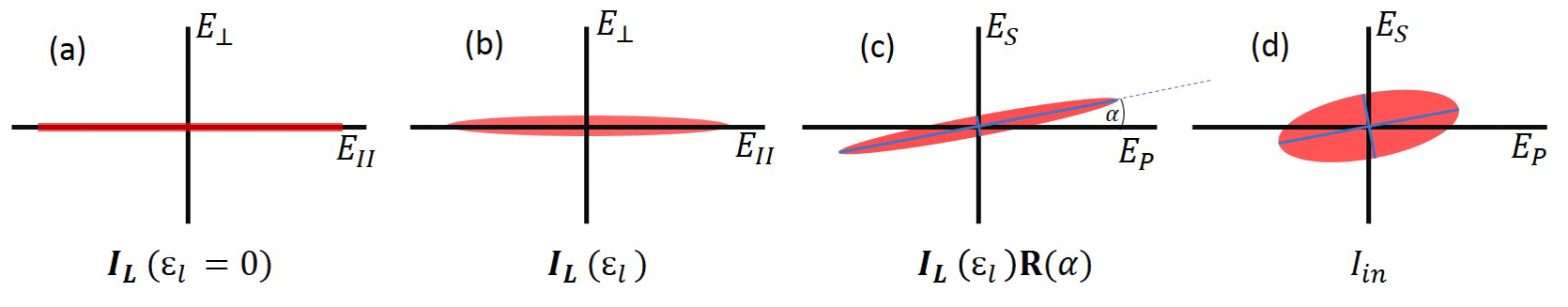
Figure 3(a) Polarization state of the light generated by the laser (100 % linearly polarized); E denotes electromagnetic field. (b) The laser radiation is elliptically polarized after passing the beam expander (see Fig. 1). (c) The receiving cross- and co-polarized signal channels (ES and EP) are usually not perfectly aligned to the main polarization plane of the laser radiation, i.e., α>0. (d) Polarization plane in the receiver for light which has been backscattered and depolarized by the atmosphere.
The transmitted radiation P0(z) of the laser pulse can be written as the sum
with the co- and cross-polarized light components, and , with polarizations parallel and orthogonal to the main plane of laser light polarization. We introduce the so-called cross-talk term εl:
which describes the small amount of cross-polarized light in the laser beam after leaving the transmission block of the lidar towards the atmosphere. Now we can write
The transmitted electromagnetic wave front is then given by the Stokes vector (Lu and Chipman, 1996).
The misalignment between the polarization axis of the transmitted light and the co-polarized receiver channel (defined by the respective polarization filter in front of the detector) is characterized by angle α and described by the rotation Müller matrix (Bravo-Aranda et al., 2016); here we adopt the notation for the trigonometric functions used in Freudenthaler (2016), i.e., cos (2α):=c2α and sin (2α):=s2α:
Then the incident field after backscattering by atmospheric particles and molecules, and before passing the receiver block, can be written as (Freudenthaler, 2016)
with the atmospheric polarization parameter
The scattering matrix F describes the interaction of the laser photons with the atmospheric particles and molecules. F11 and δ are the backscatter coefficient and the volume linear depolarization ratio, respectively.
The true volume backscatter coefficient (β:=F11) is given by
with the backscatter contributions for the co- and cross-polarization planes (with respect to the true polarization planes given by the transmitted laser pulses). The volume linear depolarization ratio is defined as
Figure 3 illustrates the different polarization states and configurations of the original laser pulses (Fig. 3a) and after leaving the beam expander as elliptically polarized laser light (Fig. 3b). The receiver block may be not well aligned to the main plain of laser radiation so that the photomultiplier measures different cross- and co-polarized signal components with respect the outgoing cross- and co-polarized laser light components in Fig. 3b. The rotated polarization axis is represented in Fig. 3c, and after being backscattered and depolarized, the incident polarization plane has the form as shown in Fig. 3d.
To distinguish the apparent measured volume backscatter coefficient, determined from the actually measured co- and cross-polarized signal components which are related to the incident field Iin (Eq. 6, see Fig. 3c), we introduce index “in” and have the following relationships and links to the (true) laser light polarization plane:
Now using Eq. (10) (describing the first term of Iin in Eq. 6) and Eq. (11) (describing the second term of Iin in Eq. 6), the apparent backscatter components and can be written as
These three backscattering components (Eqs. 10, 12, and 13) can be measured separately using the three different telescopes of our polarization lidar described in Sect. 2.
It is worthwhile to mention that polarization lidars typically have two detection channels, either a cross-polarized and a parallel-polarized channel or a cross-polarized and so-called total channel. A commonly used method for the calibration is to insert an additional polarization filter into the optical path of the receiver unit and to rotate or tilt a λ∕2 plate (Liu and Wang, 2013; Engelmann et al., 2016; McCullough et al., 2017). For these calibrations an extra measurement period is required. This calibration can introduce new and significant uncertainties (Biele et al., 2000; Freudenthaler et al., 2009; Mattis et al., 2009; Haarig et al., 2017).
As mentioned in the introduction, the concept to calibrate a lidar depolarization receiver by using three channels was proposed by Reichardt et al. (2003). The method consists of an absolute calibration procedure based on the measurement of elastically backscattered light with three detection channels for measuring co-, cross-, and totally polarized backscatter components.
To determine the number of counts that the detection channels measure, Müller matrices representing the optical path of each channel would need to be added to Eq. (6). Nevertheless, in this approach we follow the view adopted by Reichardt et al. (2003), in which the traditional lidar equation is used to characterize the lidar channels.
Let us now introduce the lidar equations for these three signals. Following Reichardt et al. (2003), the number of photons Ni that a lidar detects at height z (above the full overlap height) with channel i is given by
P0 is the number of emitted laser photons and and are the optical efficiencies regarding the co- and cross-polarized components ( and ) of the backscattered light that arrives at the channel-i detector. These efficiencies include instrumental constants that contain the total transmittance through all optical components and gain of the detectors and attenuation in the path of each channel. T denotes the atmospheric single-path transmission and is the same for all three detection channels (co-, cross-, and total) since the extinction is independent of the state of polarization of the light. Rearrangements lead to the following versions of the lidar equations for the cross- (S) and co-polarized (P) channels:
or
Here Di denotes the so-called efficiency ratio (Reichardt et al., 2003), and it is defined as
The absence of optical elements before the polarization filters (such as the telescope itself and beam splitters) avoids further polarization effects, such as diattenuation and retardation, described in detail by Freudenthaler (2016). Moreover, since we employed the same filter model in the optical path of the channels P and S, we assumed that . In the case of the total signal component (i=tot) we assume that Dtot=1 and we introduce the overall efficiency ηtot for simplicity reasons. The numbers of photons measured with each of the three channels (i=P, S, tot) are then given by
After further rearranging we finally obtain
To consider, in the next step, receiver misalignment and cross-talk effects, we introduced the parameters (Eq. 2), describing the small amount of cross-polarized light in the laser beam after leaving the transmission block into the atmosphere, and the rotation angle α describing the angular misalignment between the transmitter and receiver units. To also consider the receiver–channel cross talk, we further introduce εr, defined by . The receiver cross-talk value is typically (according to the filter manufacturer) as here the only element to consider is the polarization filter in front of the telescopes. Now combining Eqs. (10), (12), and (13) with Eqs. (21)–(23), we can write
Until this point, the analytical procedure has been based on the assumption that the polarization filters in front of the cross- and co-polarized telescopes are pointing 90∘ with respect to each other. However, in the general case, when their angular deviation with respect to their respective components is different (EP to E∥ and ES to E⟂), Eqs. (24) and (25) have a different angular component. In this approach, we keep this assumption for the development of a simple calibration procedure. In Appendix A, the general case is evaluated (angle P to ), and based on a measurement example, we demonstrated that the impact of this assumption can be neglected in our system.
3.2 Determination of calibration constants and the volume linear depolarization ratio
Outgoing from Eqs. (24)–(26) we will define instrumental (interchannel) constants which are required to calibrate the lidar in the experimental practice and which are also used in the determination of the volume linear depolarization ratio. The equations for the determination of the depolarization ratios will be given. Three different ways can be used to determine the linear depolarization ratio profiles.
Considering Eq. (26) and the sum of Eqs. (24) and (25), we can write
Equation (27) is independent of the transmission cross-talk factor εl and of the rotation of the receiver axis (and thus rotation angle α) but depends on the receiver cross-talk factor εr.
Let us introduce the interchannel instrumental constants
and the signal ratios RP, RS, and Rδ
By using these definitions, Eq. (27) (after multiplication with ) can be rearranged to
Equation (34) is only valid for the case of an almost ideal polarization lidar receiver unit, i.e., when . This is not the case for most lidar systems in which the receiver and separation unit may introduce differences between the transmission ratios and DP. In the next step, we form the difference of Eq. (34) for altitude zj minus Eq. (34) for altitude zk and obtain
In the same way, when Eq. (27) is multiplied by and , we can derive Eqs. (36) and (37), respectively.
t denotes time.
In the conventional three-signal calibration approach, each signal is normalized to a reference altitude; by doing so the efficiencies of the three channels , , and ηtot cancel themselves from the equations. Then the ratios between the three normalized signals are calculated. The retrieval of the volume depolarization ratio is performed by solving a system of two equations and two unknowns: the volume depolarization ratio at a reference height δ(z0) and the volume depolarization ratio at all heights δ(z) (Reichardt et al., 2003).
In this extended three-signal calibration procedure, the signals are not normalized to a reference height z0; instead, we directly divide the signals, obtaining the ratios RP, RS, and Rδ. By then taking the difference between two altitudes (and not the ratio) we subtract the cross talk in the emission and reception (εl and εr) and the angular misalignment (c2α). The difference additionally offers a better performance in terms of error propagation compared to the ratio. In this way, the so-called interchannel constants (Xδ, XS, and XP) remain in the equations and they can be estimated by evaluating Eqs. (35), (36), and (37), respectively. Although we can estimate these three constants, we have to note that the number of unknowns are actually two XP and XS, with the third constant Xδ being the ratio of them (please see Eq. 30); i.e., Eq. (35) is equivalent to Eq. (36) divided by Eq. (37).
Given the form of Eqs. (35)–(37), observable differences between the height points zj and zk are needed for its evaluation. In practice, only altitude regions should be selected in the determination of XP, XS, and Xδ where significant changes in the depolarization ratio occur, e.g., in liquid-water clouds in which multiple scattering by droplets produces steadily increasing depolarization with increasing penetration of laser light into the cloud (Donovan et al., 2015; Jimenez et al., 2017, 2018). Long measurement periods should be considered for the evaluation of Eqs. (35)–(37). All pairs of data points (zj and zk in a certain height range, defined according to the ratio of signals) in all single measurements (in time t) provide an array with many observations of the interchannel constants. Averaging these arrays we obtain a trustworthy estimate of these constants for the retrieval of the volume depolarization ratio (please see Fig. 6).
To derive the linear depolarization ratio, we divide Eq. (25) by Eq. (24).
Furthermore, we introduce the total cross-talk factor ξtot,
which takes account of the combined effect of the emitted elliptically polarized wave front εl, of the angular misalignment between emitter and receiver (described by the rotation angle α), and of the cross talk among receiver channels described by εr. The factor ξtot would be equal to 1 if the emitted laser pulses are totally linearly polarized, misalignment of the receiver unit could be avoided, and cross talk among receiver channels would be negligible.
Now Eq. (38) can be rewritten after dividing the numerator and denominator by and rearranging the equation:
and the volume depolarization ratio can be obtained from Eq. (40) after rearrangement,
As shown in Eq. (41), the volume depolarization ratio can be calculated by using the ratio Rδ between the cross- and co-polarized signals and when the constants Xδ and ξtot are known. As a first step of the calibration, the interchannel constant Xδ (together with XP and XS) is obtained from the measurements by evaluating Eqs. (35)–(37) in the selected height range (with variations in the depolarization) at each measurement time t. Then ξtot can be estimated in a region (defined by height zmol) with dominating Rayleigh backscattering for which the volume depolarization ratio, δmol, is assumed as constant and known. Behrendt and Nakamura (2002) theoretically estimated a value of the linear depolarization ratio caused by molecules of 0.0046 for a lidar system whose interference filters have a full width at half maximum (FWHM)=1.0 nm. However, Freudenthaler et al. (2016) have found a value of 0.005±0.012 based on long-term measurements in aerosol and cloud-free tropospheric height regions. We used this value and we have considered the propagation of this systematic uncertainty in our calculations. Thus, from Eq. (41) ξtot is given by
By calculating the ratio between Eqs. (24) and (26) (co to total) or the ratio between Eqs. (25) and (26) (cross- to total), the volume depolarization ratio can also be derived:
In summary, the volume linear depolarization ratio can be calculated after the determination of the constants XP, XS, Xδ, and ξtot. Then the signal ratio profiles RP(z), RS(z), and Rδ(z) are required and calculated within Eqs. (31), (32), and (33), and by considering Eqs. (41), (43), and (44) the depolarization ratio can finally be calculated by using the pair of signals NS and NP, the pair NS and Ntot, or the pair NP and Ntot, respectively. However, the expected errors in the retrievals are not the same for all of these pairs since they present different sensitivities to changes in the depolarization ratio, obtaining the largest uncertainties when the pair NP and Ntot is used.
4.1 Application of the calibration approach to a measurement case
To test the method introduced in Sect. 3, the measurement case from 19 September 2017 was analyzed and the results are presented in this section. Figure 4 provides an overview of the atmospheric situation. An aerosol layer reached up to about 2.8 km in height and was topped by a persistent, shallow altocumulus deck with a cloud base height at 2.6–2.7 km a.g.l. (above ground level).
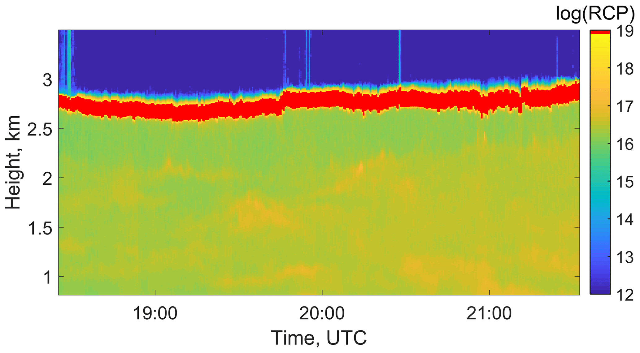
Figure 4Range-corrected 532 nm total backscatter signal (RCP) measured on 19 September 2017 with 30 s and 7.5 m vertical resolution.
Although the time resolution of the lidar measurements is 30 s, to reduce computing time and signal noise, we consider 5 min average measurements. Figure 5 shows the three range-corrected signals of the polarization lidar, the signal ratios as defined by Eqs. (31)–(33), and the corresponding inverse ratios for a 5 min measurement as an example.
In the next step of the data analysis and calibration procedure, we selected the height range from a few meters below cloud base up to 240 m above cloud base for each 5 min averaging period t. Then we computed the instrumental interchannel ratios , , and with Eqs. (37), (36), and (35), respectively. Height resolution was 7.5 m. The result is shown in Fig. 6.
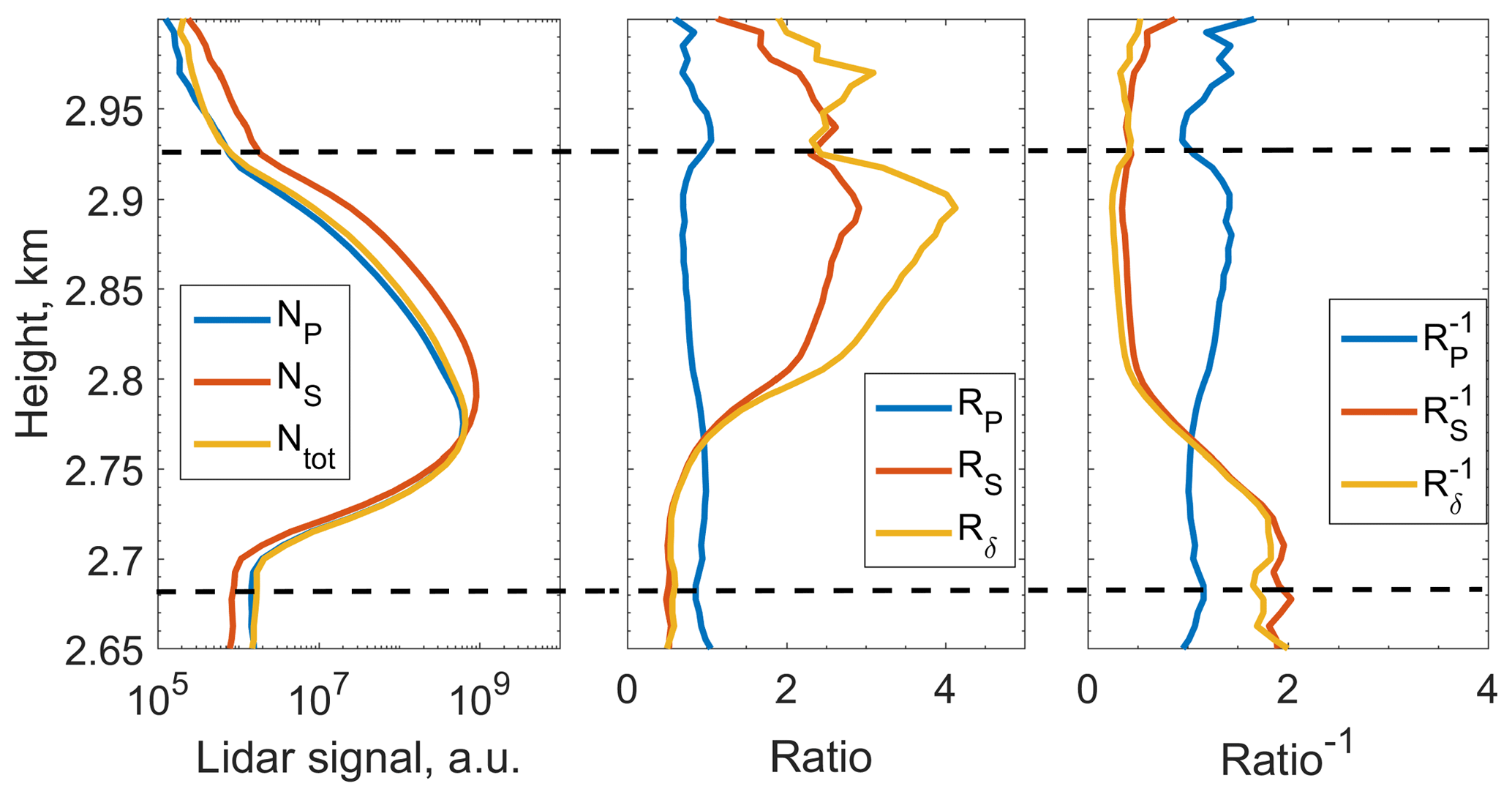
Figure 5Example of a 5 min profile of range-corrected lidar signals from the channels, signal ratios, and inverse ratios. The calibration procedure considers all signals of the 3 h measurement period shown in Fig. 4. The dashed line indicates the range in which the calibration calculations were carried out.
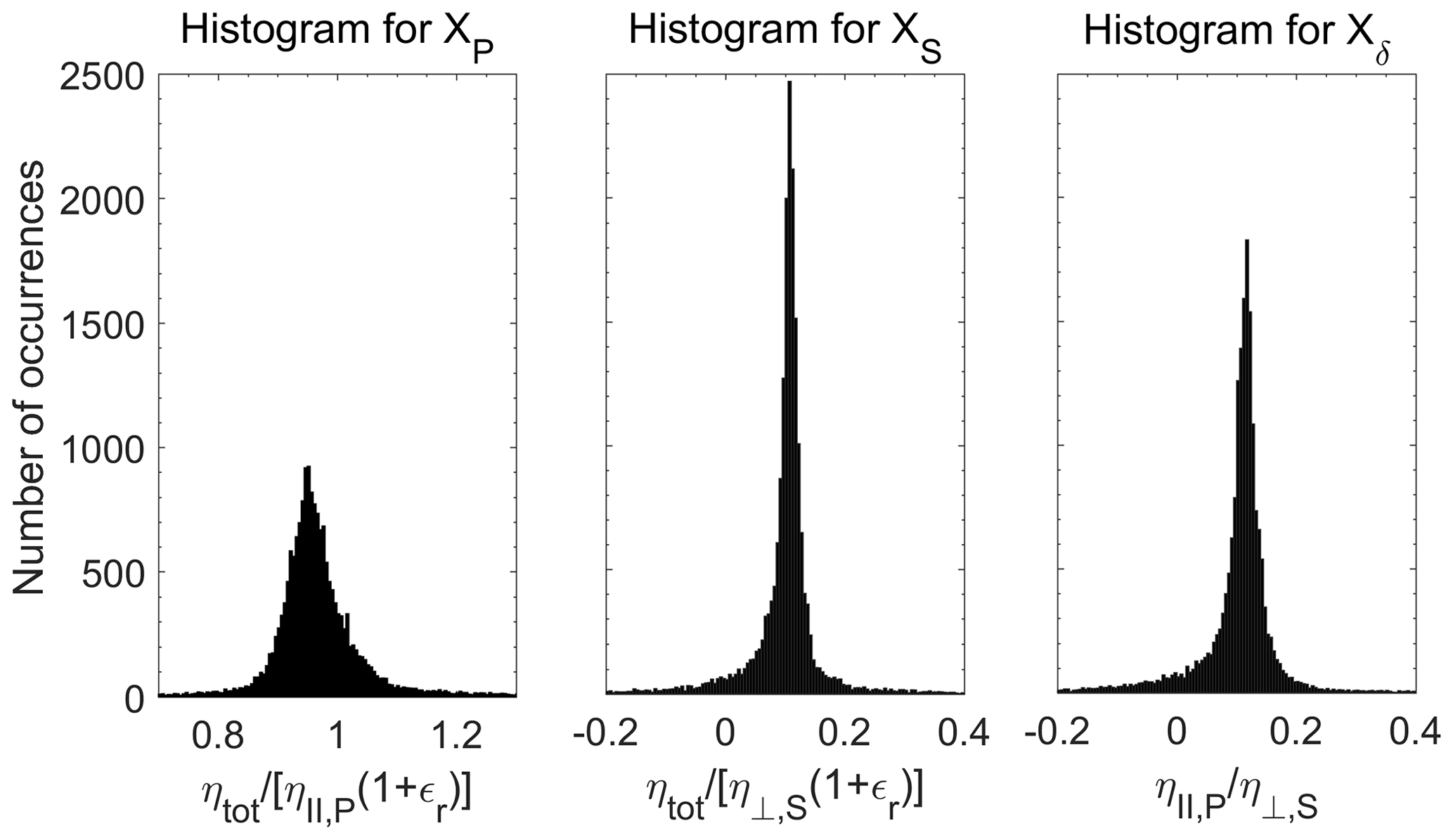
Figure 6Histograms for the interchannel constants XP, XS, and Xδ. Each point corresponds to a combination of zj and zk in a 5 min period, obtaining about 18 000 data points for this 3 h measurement case.
The mean values of the constants with the respective statistical error based on Fig. 6 are , , and . The reason for these low uncertainties is that the calibration is performed in a cloudy region so that every channel shows high count rates and thus high signal-to-noise ratios.
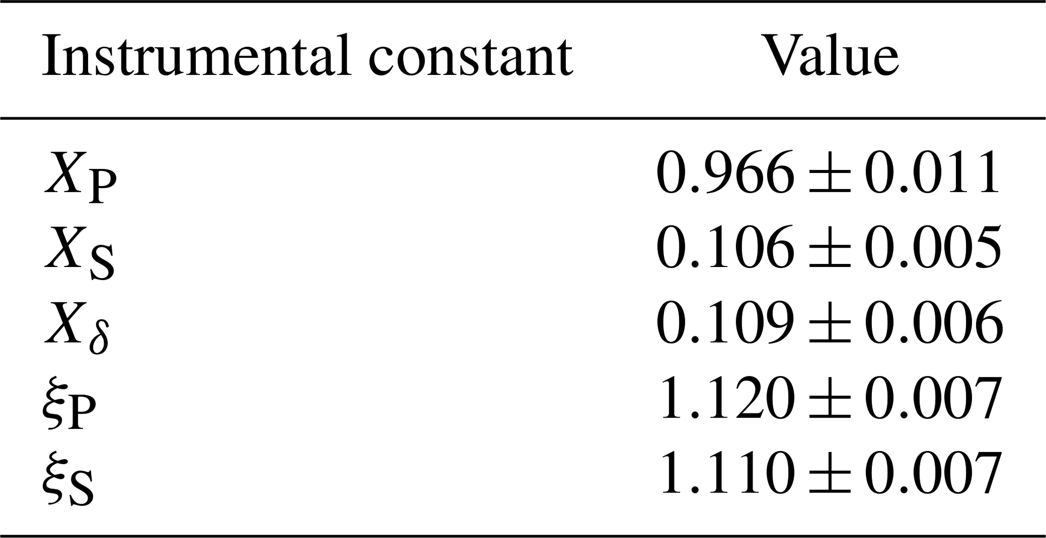
Using the constant Xδ and evaluating Eq. (42) in the particle-free region of the 3 h measurement period, a mean value of for the total cross talk was obtained. Given the form of the equations to retrieve the profiles of volume depolarization ratio (Eqs. 35–37), the propagated uncertainty associated with ξtot does not vary largely with height, which leads to a large percentage uncertainty on the retrieval of the volume linear depolarization ratio in the region with low depolarization ratios, also characterized by low signal strengths. Table 1 summarize the retrieved instrumental constants for the measurement case presented.
Table 1Values of the instrumental interchannel constants and cross-talk factor determined for the measurement case presented.
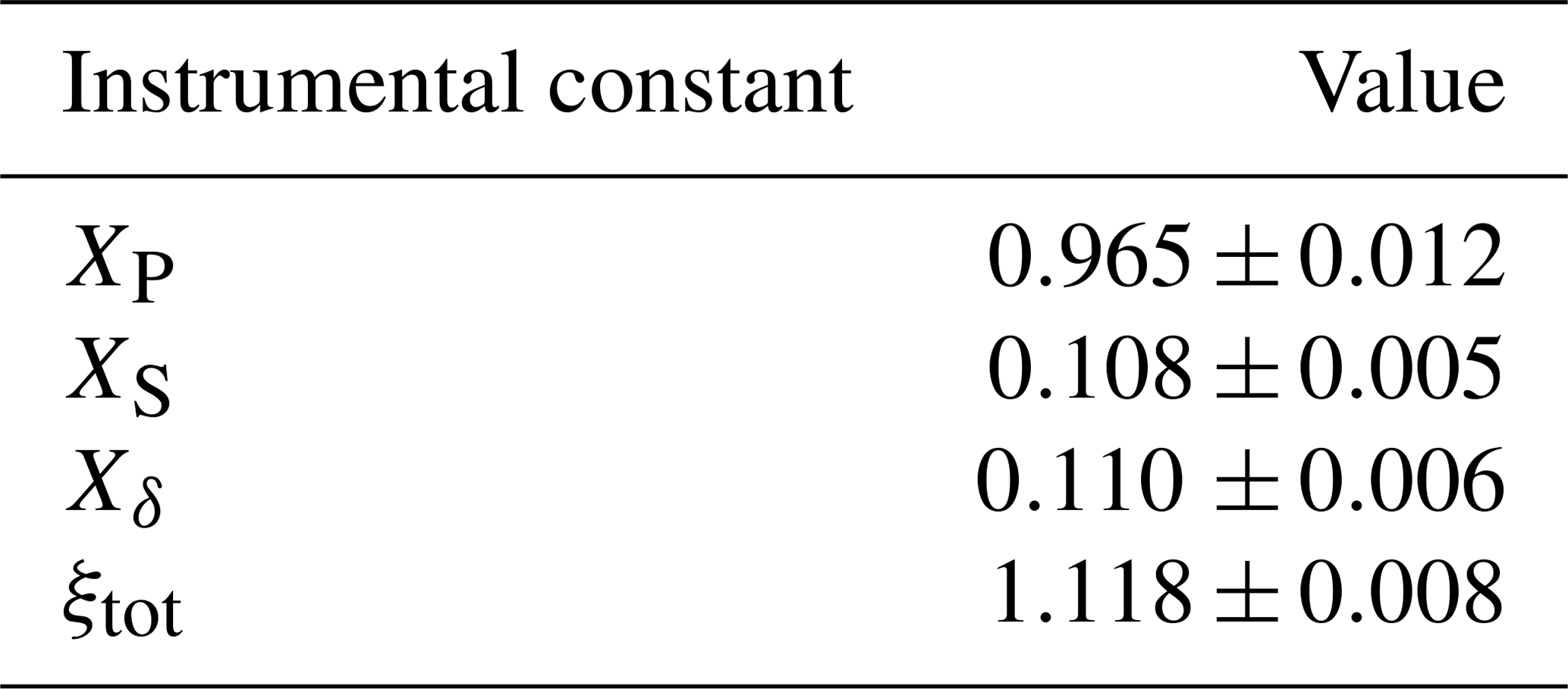
Figure 7 presents the height profiles of the volume linear polarization ratio computed by means of Eqs. (41), (43), and (44). Good agreement among the different solutions is visible. However, the depolarization ratios obtained from the channels NP and Ntot (blue) show the largest uncertainties, especially above the cloud layer. The profile-mean absolute uncertainties from the ground up to the cloud top (3.1 km) for δ(RP,XP), δ(RS,XS), and δ(Rδ,Xδ) are 0.034, 0.0139, and 0.0137, respectively. The three derived depolarization ratios agree well in the cloud region. Differences appear in the upper part of the cloud caused by strongly reduced count rates due to the strong attenuation of all the channels, in order to avoid signal saturation at low level clouds.
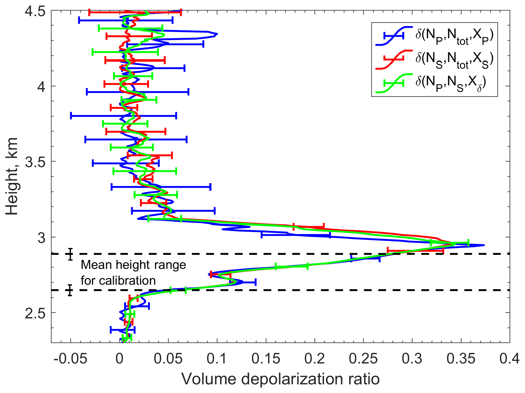
Figure 7Profiles of the volume linear depolarization ratio for the 3 h period in the cloud region, using the three pairs of signal ratios presented in Eqs. (41), (43), and (44). The error bars include the statistical and systematical uncertainties. The dashed lines indicate the mean height range (of 240 m) at which the calculation of the interchannel constants was performed.
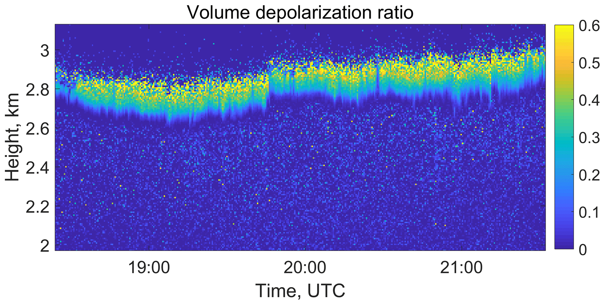
Figure 8Volume linear depolarization ratio for the entire 3 h period, shown in Fig. 4. The temporal resolution is 30 s.
Figure 8 presents the volume depolarization ratio with 30 s temporal resolution. The signal ratio Rδ and the constant Xδ were used. These profiles are the basis for the retrieval of the microphysical properties of the liquid-water cloud. The results will be discussed in a follow-up article (Jimenez et al., 2019).
To validate the new system and the calibration procedure a comparison among the measurements of the volume linear depolarization ratio with the lidar systems MARTHA and BERTHA (Backscatter Extinction Lidar Ratio Temperature and Humidity profiling Apparatus) is presented in Fig. 9. The observations were conducted at Leipzig (51∘ N, 12∘ E) on 29 May 2017 with the presence of a dust layer between 2 and 5 km and a cirrus cloud at 11 km (see Fig. 9a). Good agreement in the dust layer can be noted, while the cirrus cloud shows differences between the two systems. That difference can be attributed to the fact that the BERTHA system is pointing 5∘ with respect to the zenith, while the MARTHA system points to the zenith (0∘). This could lead to specular reflection by horizontally oriented ice crystals reducing the depolarization ratio in the case of the MARTHA system.

Figure 9Volume linear depolarization ratio obtained with MARTHA (extended three-signal method) and BERTHA (Δ90∘ method) on (a) 29 May 2017, 20:20–20:45 UTC (with smooth 27 bins) and (b) 22 August 2017, 20:45–23:15 UTC (Haarig et al., 2018). The systems were calibrated independently. The systems were located at a distance of 80 m.
A second measurement period during a unique event with a dense biomass burning smoke layer in the stratosphere on 22 August 2017 was considered for comparison (Haarig et al., 2018). Here very good agreement for the layer between 5 and 7 km and also for the layer at 14 km was obtained, confirming the good performance of the systems and of the respective calibration procedures, extended three-signal method in MARTHA, and Δ90∘ method in the BERTHA system.
4.2 Temporal stability of the polarization lidar calibration and performance
The time series of the interchannel constant Xδ obtained from MARTHA observations between days 120 and 320 of 2017 is presented in Fig. 10. The respective time series of ξtot is given in Fig. 11. As can be seen, the calibration values show the lowest uncertainties in the interchannel constants (of about 4 %) when altocumulus layers with a stable cloud base and moderate light extinction were present. Higher uncertainty levels were observed in the case of cirrus clouds (green, 11 %) and the Saharan dust layer (red, 17 %). In the case of very thick cumulus clouds (black), the mean uncertainty was 21 %. One reason for these differences in the uncertainty of Xδ is that the system was optimized for the observation of low-altitude liquid-water clouds, for which the detection channels need large attenuation to avoid saturation of the detectors in the cloud layer. This setup prohibited an optimum detection of high-level dust layers and ice clouds due to the low signal strength for these cases. Furthermore, liquid clouds are favorable for calibration because the volume depolarization ratio increases very smoothly as a result of the increasing multiple scattering impact. At these conditions, a large number of measurement pairs for heights zj and zk with different depolarization ratios are available. Some slight changes of Xδ occurred when the attenuation configuration of the polarization receivers was changed. Small day-to-day changes were caused by small variations in the response of each detector with time.
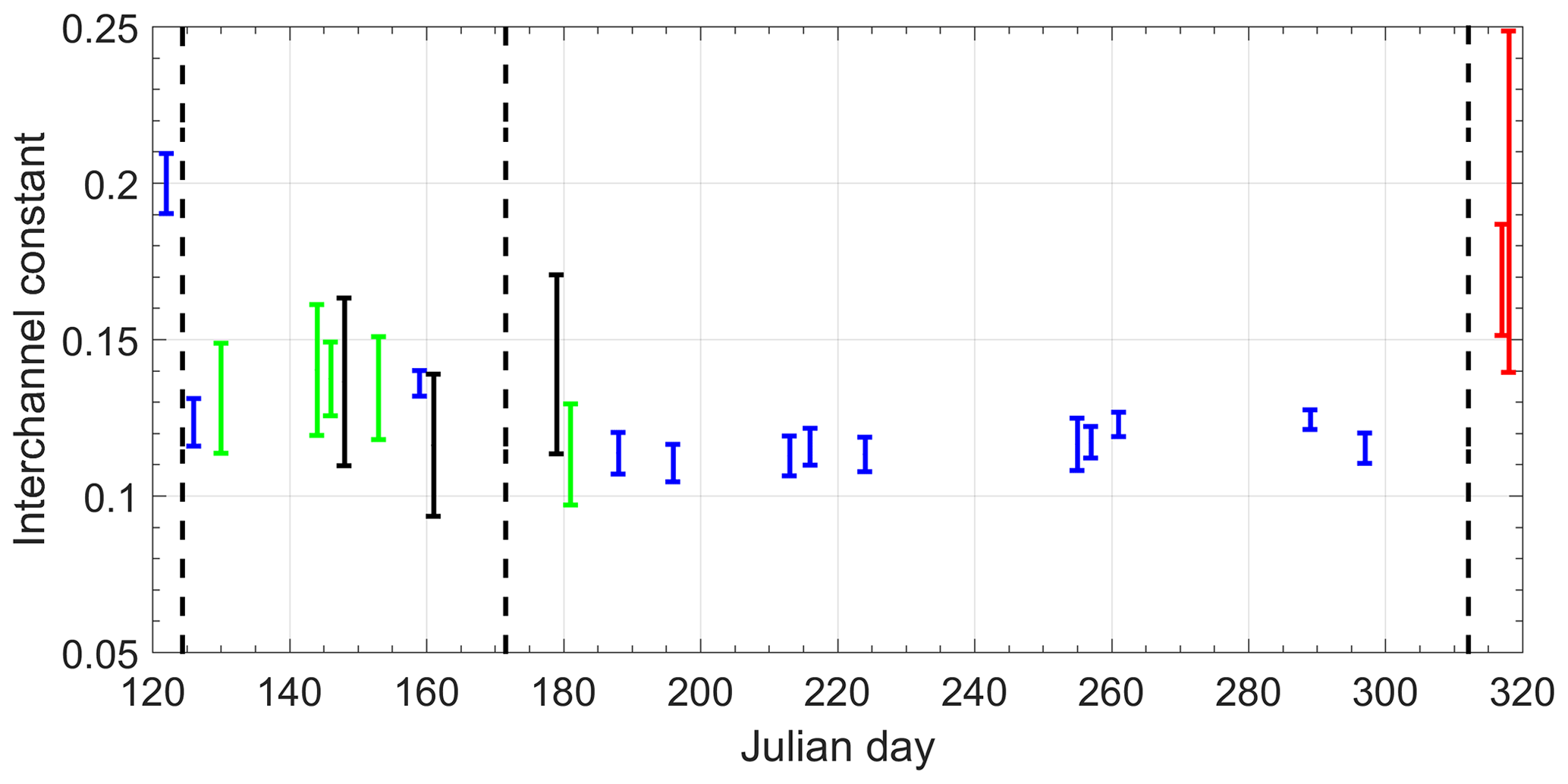
Figure 10Time series of the interchannel calibration constant Xδ measured from the end of April to mid-November 2017. The vertical bars show the uncertainty in the retrieval. The calibration procedure was based on lidar measurements in liquid-water clouds (blue) and cirrus clouds (green) and during optically thick cumulus events (black) and Saharan dust periods (red). The dashed lines indicate the days when changes in the attenuation configuration of the channels were made.
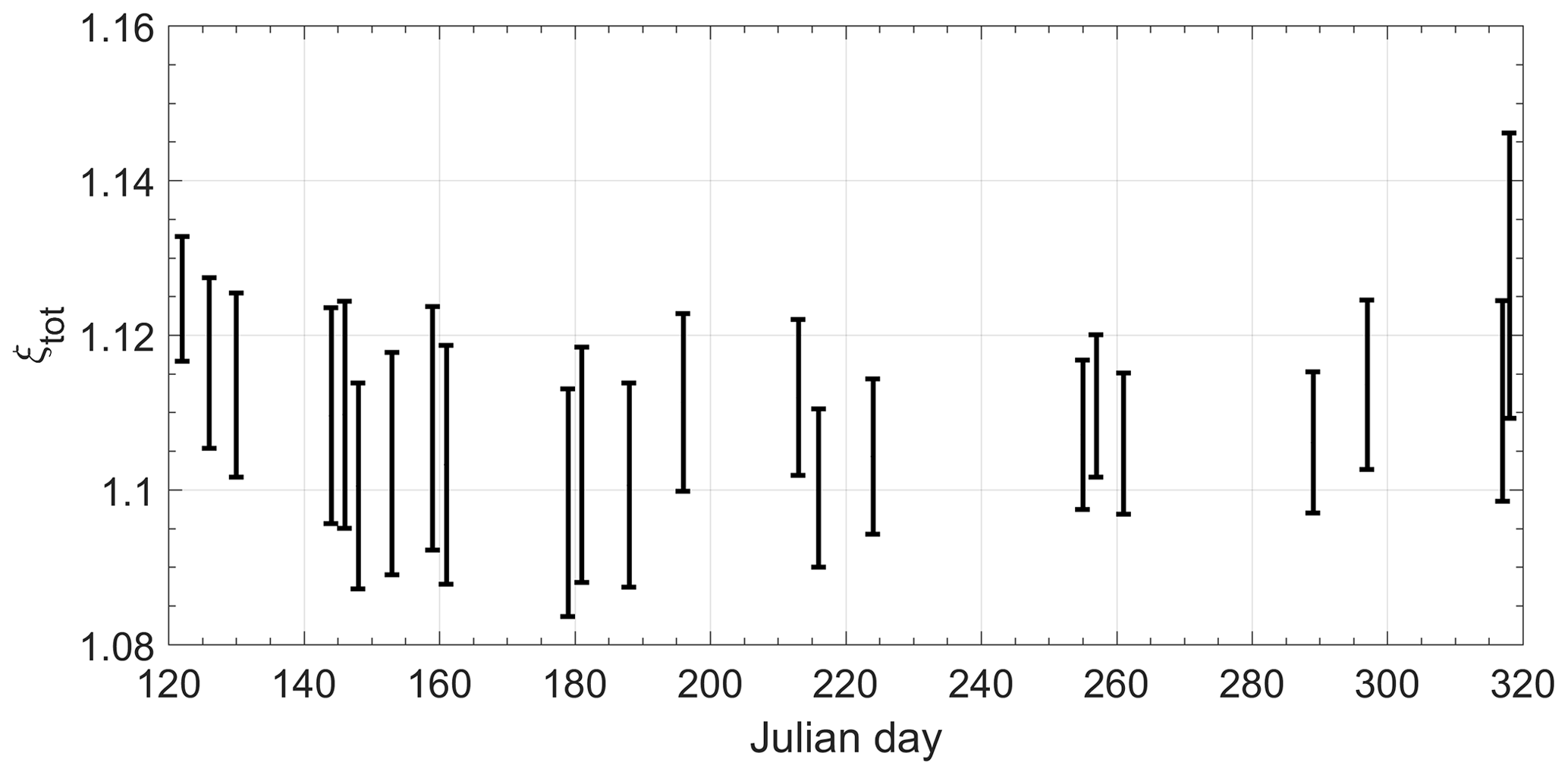
Figure 11Time series of the total cross-talk factor ξtot measured in 2017. The vertical bars show the uncertainty in the retrieval, which includes the statistical error from the determination of the interchannel constants and systematical errors from the value considered in the molecular region 0005±00012.
In Fig. 10 the retrieved values of ξtot are shown; small variations can be seen but they remain much lower than the uncertainties, and no stronger variations can be noted with changes in the attenuation or changes of the calibration medium (water cloud, cirrus, Saharan dust layer). In 2017, the mean value .
In this work a new formalism to calibrate polarization lidar systems based on three detection channels has been presented. We propose a simple lidar polarization receiver, based on three telescopes (one for each channel) with a polarization filter on the front (in the case of the cross- and co-polarized channels). This setup removes the effect of the receiver optics on the polarization state of the collected backscattered light, simplifying the measurement concept. The derivation of the volume linear depolarization ratio considering the instrumental effects on the proposed system was described in Sect. 3. Here there are three effects considered: the emitted laser beam (after beam expander) is slightly elliptically polarized (εl), there is an angular misalignment (α) of the receiver unit with respect to the main polarization plane of the emitted laser pulses, and there is a small cross-talk amount in the detection channels (co- and cross-) (εr). These instrumental parameters can be summarized into one single constant, the so-called total cross talk (ξtot).
The methodology does not require a priori knowledge about the behavior of the instrument in terms of polarization and permits the determination of the so-called interchannel constants XP,XS, and Xδ, which depend on the attenuation and detector response of each channel, and thus it is expected to vary among different measurement days. In the free-aerosol region the total cross talk can also be estimated by means of long-term measurements. In our case we estimated a mean value of . The calibration is based on actual lidar measurement periods, providing large numbers of input data for accurate estimation of the mean value of the instrumental constants. However, it needs a strong depolarizing medium for its application, such as dust layers and also water clouds, which depolarize the light due to multiple scattering in droplets or due to single scattering of ice particles.
A case study of a liquid-water cloud observation was presented. The 3 h period demonstrates the potential of the new technique for the retrieval of accurate high-temporal-resolution depolarization profiles. The method is simple to implement and allows high-quality depolarization ratio studies. Temporal studies indicated the robustness and stability of the three-signal lidar system over long time periods. A comparison with a second polarization lidar shows excellent agreement regarding the derived volume linear polarization ratio of biomass burning smoke throughout the troposphere and the lower stratosphere up to 16 km in height.
The lidar data used for this research can be accessed by request to the Leibniz Institute for Tropospheric Research.
For the derivation outlined in Sect. 3 it is assumed that the polarization filters in front of the cross- and co-polarized telescopes are pointing 90∘ with respect to each other. However, in the general case, when their angular deviation with respect to their respective components is different (EP to E∥ and ES to E⟂), Eqs. (24) and (25) have a different angular component. In this Appendix we analyze this general case and discuss the need of implementation depending on the results obtained.
We define the angles αP and αS as the angular misalignment of the channels EP and ES with respect to E∥ and E⟂, respectively (see Fig. A1). We rewrite Eqs. (24)–(26), we factorize by (1+εr), and to simplify the expression we adopt the polarization parameter again. We do not use the short notation of the cosine adopted in Sect. 3.
In a way similar to how we defined ξtot, we define the total cross-talk factor for the co- and cross-polarized channels.
The three-signal polarization equation (Eq. 27) can be rewritten in a general form, when adding Eqs. (A1) and (A2) and considering Eq. (A3):
The term depends on the difference of the cosines of 2αP and 2αS. We define the parameter , which accounts for the difference of the impact of the polarization channels.
This factor can be positive or negative, depending on which polarization filter is more misaligned, and it is equal to zero when they point 90∘ with respect to each other. Equation (A6) can be expressed as
We adopt the notation
to account for the difference among the signal ratios RP, RS, and Rδ, between the polarization parameter a, and between the ratios a∕RS and a∕RP at the heights zj and zk. In an way equivalent to how we derived Eqs. (35)–(37) we can obtain a general solution for the instrumental interchannel constants:
In an absolute sense it would not be possible to determine the interchannel constants XP, XS, and Xδ without knowing the polarization parameter (or the depolarization ratio); however, the impact on Eqs. (A10)–(A12) of their respective second term can be very small since it depends on the difference of the cosines of small angles, for example, if and , using Eq. (A7) . Considering this small effect, a first guess of the polarization parameter would be sufficient to solve Eqs. (A10)–(A12).
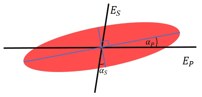
Figure A1Scheme of the observation of the polarization state of the backscattered light (similar to Fig. 3). The co-polarized and cross-polarized channels are misaligned with respect to their components at angles αP and αS, respectively.
Calculating the three ratios among Eqs. (A1), (A2), and (A3), we can obtain the volume linear depolarization ratio, similarly to how it was performed for Eqs. (41), (43), and (44).
In the measurement example presented, we performed an iterative computation procedure to determine the interchannel calibration constants and the cross-talk factors. Using Eqs. (A10)–(A12), in a first run we determined the interchannel constants when we assume , i.e., αP=αS. A first guess of the volume depolarization ratio using each pair of signals is obtained (Eqs. A13–A15), and then the corresponding cross talks ξP and ξS are determined by imposing a mean value of in the free-aerosol region (Freudenthaler et al., 2016b). The second run takes the values of and of the polarization parameter a(z,t) (Eqs. A14 and A16) from the first run and the interchannel constants are computed again. Figure A2 shows the results of performing the calibration iteratively. Small differences between the values obtained in the first and second run can be noted; in fact, the variations are smaller than the error of the respective constants, and we can see that after the second run, all values remain practically constant. The mean values of the instrumental constants after six iterations are listed in Table A1.
In this measurement case we found a value for . Due to this small value there are no important variations between the first guess and the second run; therefore we conclude that by assuming a fast and practical inversion procedure is possible. However, in cases with larger differences between αP and αS, an iterative procedure as described above would be needed.
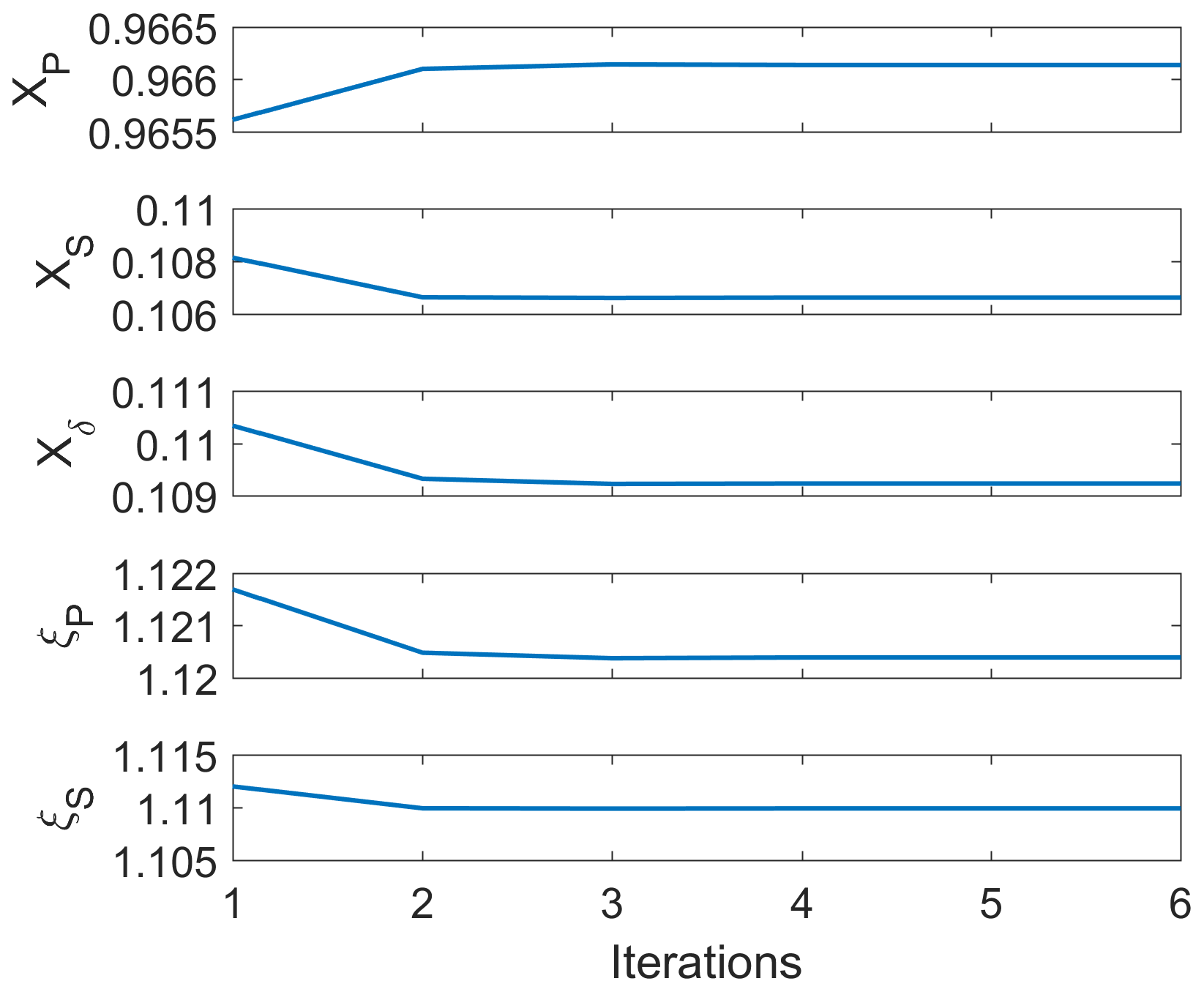
Figure A2Instrumental channels obtained with an iterative procedure. We did not include the error bars since they are much larger than the variations among runs.
This general solution for the lidar three-signal problem converges to the same results when we also consider that the receiver cross talk can eventually be different for the channels P and S. In that case we would have εr,P and εr,S, which would also lead to two constants ξP and ξS to determine. For simplicity this section only discussed the effect of the different angular misalignment of channels P and S.
Table A1Results of the instrumental constants after using the iterative procedure (six runs).
| z | Height. |
| a | Atmospheric polarization parameter. Varies with height z. |
| δ | Atmospheric volume depolarization ratio, so that . |
| δmol | Volume depolarization ratio in the free-aerosol region. Assumed constant and known. |
| β | Backscattering coefficient. Equal to the element F11 from the atmospheric scattering matrix. |
| βin | Backscatter that arrives at the receiver and it is measured by the total channel βin=β in our system (Dtot=1). |
| Parallel component of the arriving backscatter. | |
| Cross component of the arriving backscatter. | |
| T | Atmospheric transmission path for the lidar equation. |
| P0 | Number of emitted photons. |
| εl | Portion of the emitted radiation polarized in the cross direction (⊥), called cross talk of the emitter. |
| IL | Stokes vector describing the emitted radiation in terms of the polarization state. |
| F | Scattering matrix of the atmosphere. The element F11 corresponds to the backscattering coefficient β. |
| Iin | Stokes vector describing the arriving radiation after being transmitted, backscattered, and depolarized by the atmosphere. |
| c2α | cos (2α), α denotes the rotation between the polarization axis of the emission with respect to the reception. |
| R(α) | Rotation matrix to consider the effect of the rotation α between emission and receiver polarization plane. |
| Ni(z) | Number of photons measured by each detector (i=P, S, tot) at height z. |
| Constant describing the efficiency of channel P to component ∥. | |
| Constant describing the efficiency of channel S to component ⟂. | |
| ηtot | Constant describing the efficiency of the total channel (tot) to the sum of the components . |
| Di | Efficiency ratio of each channel (i=P,S ). Dtot≡1 (ideal). |
| εr | So-called cross talk of the receiver. (ideal case). |
| XP | So-called interchannel constant, similar to the gain ratio used in previous studies (η∗). . |
| XS | . |
| Xδ | . |
| RP | Ratio of signals NP(z)∕Ntot(z). |
| RS | Ratio of signals NS(z)∕Ntot(z). |
| Rδ | Ratio of signals NS(z)∕NP(z). |
| ξtot | So-called total cross talk of the system (ideal case). It summarizes the three instrumental effects considered (εl,c2α and εr). |
| ξP | Total cross talk of the P channel (nonideal case). |
| ξS | Total cross talk of the S channels (nonideal case). |
| . | |
| ΔRi(zj,zk) | . |
Additional information about the extended three-signal calibration approach
-
The extinction coefficient is assumed to be independent of the polarization state of the light. This assumption permits the simplification of the three lidar equations, making possible the determination of the instrumental constants.
-
The effects of the emission and reception in terms of polarization can be summarized into one total cross-talk constant ξtot (in the ideal case), or into two total cross talk constant ξP and ξS for the nonideal case (Appendix A).
-
Differences with previous studies in terms of the nomenclature are present:
- •
-
In our approach ε denotes cross talk, and not the error angle of the Δ90 calibration as denoted in previous studies. The cross talk has usually been denoted by GS and HS (Freudentaler, 2016).
- •
-
Di denotes the efficiency ratio (Reichardt et al., 2003), while in recent studies D denotes the diattenuation parameter.
The total channel is assumed to be ideal in terms of polarization, i.e., Dtot=1.
-
No diattenuation and retardation are considered in the emission and reception units.
The theoretical framework was developed by CJ in close cooperation with AA, MH, and UW. RE, JS, and CJ contributed in the setup of the lidar instrument. CJ wrote the computing code for the analysis. CJ and MH performed the measurements and analyzed the data of the MARTHA and BERTHA systems, respectively. CJ and AA prepared the paper in cooperation with MH.
The authors declare that they have no conflict of interest.
This research was partially funded by the program DAAD/Becas Chile, grant no. 57144001. This activity is supported by the ACTRIS Research Infrastructure (EU H2020-R&I), grant agreement no. 654109.
We thank Ilya Serikov for the fruitful discussions on the topic. We would
like to acknowledge the three anonymous referees for their valuable feedback given during
the revision process.
The publication of this article was funded by the
Open Access Fund of the Leibniz Association.
Edited by: Vassilis Amiridis
Reviewed by: three anonymous referees
Behrendt, A. and Nakamura, T.: Calculation of the calibration constant of polarization lidar and its dependency on atmospheric temperature, Opt. Express, 10, 805–817, 2002.
Belegante, L., Bravo-Aranda, J. A., Freudenthaler, V., Nicolae, D., Nemuc, A., Ene, D., Alados-Arboledas, L., Amodeo, A., Pappalardo, G., D'Amico, G., Amato, F., Engelmann, R., Baars, H., Wandinger, U., Papayannis, A., Kokkalis, P., and Pereira, S. N.: Experimental techniques for the calibration of lidar depolarization channels in EARLINET, Atmos. Meas. Tech., 11, 1119–1141, https://doi.org/10.5194/amt-11-1119-2018, 2018.
Biele, J., Beyerle, G., and Baumgarten, G.: Polarization lidar: Corrections of instrumental effects, Opt. Express, 7, 427–435, 2000.
Bravo-Aranda, J. A., Belegante, L., Freudenthaler, V., Alados-Arboledas, L., Nicolae, D., Granados-Muñoz, M. J., Guerrero-Rascado, J. L., Amodeo, A., D'Amico, G., Engelmann, R., Pappalardo, G., Kokkalis, P., Mamouri, R., Papayannis, A., Navas-Guzmán, F., Olmo, F. J., Wandinger, U., Amato, F., and Haeffelin, M.: Assessment of lidar depolarization uncertainty by means of a polarimetric lidar simulator, Atmos. Meas. Tech., 9, 4935–4953, https://doi.org/10.5194/amt-9-4935-2016, 2016.
Chipman, R. A.: Mueller matrices in: Handbook of Optics, Volume I, 3rd edn., chap. 14, McGraw-Hill, 2009.
David, G., Miffre, A., Thomas, B., and Rairoux, P.: Sensitive and accurate dual-wavelength UV-VIS polarization detector for optical remote sensing of tropospheric aerosols, Appl. Phys. B, 108, 197–216, https://doi.org/10.1007/s00340-012-5066-x, 2012.
Donovan, D. P., Klein Baltink, H., Henzing, J. S., de Roode, S. R., and Siebesma, A. P.: A depolarisation lidar-based method for the determination of liquid-cloud microphysical properties, Atmos. Meas. Tech., 8, 237–266, https://doi.org/10.5194/amt-8-237-2015, 2015.
Engelmann, R., Kanitz, T., Baars, H., Heese, B., Althausen, D., Skupin, A., Wandinger, U., Komppula, M., Stachlewska, I. S., Amiridis, V., Marinou, E., Mattis, I., Linné, H., and Ansmann, A.: The automated multiwavelength Raman polarization and water-vapor lidar PollyXT: the neXT generation, Atmos. Meas. Tech., 9, 1767–1784, https://doi.org/10.5194/amt-9-1767-2016, 2016.
Fan, J., Wang, Y., Rosenfeld, D., and Liu, X.: Review of Aerosol-Cloud Interactions: Mechanisms, significance, and Challenges, J. Atmos. Sci., 73, 4221–4252, https://doi.org/10.1175/JAS-D-16-0037.1, 2016.
Freudenthaler, V.: About the effects of polarising optics on lidar signals and the Δ90 calibration, Atmos. Meas. Tech., 9, 4181–4255, https://doi.org/10.5194/amt-9-4181-2016, 2016.
Freudenthaler, V., Esselborn, M., Wiegner, M., Heese, B., Tesche, M., Ansmann, A., Müller, D., Althausen, D., Wirth, M., Fix, A., Ehret, G., Knippertz, P., Toledano, C., Gasteiger, J., Garhammer, M., and Seefeldner, M.: Depolarization ratio profiling at several wavelengths in pure Saharan dust during SAMUM 2006, Tellus B, 61, 165–179, https://doi.org/10.1111/j.1600-0889.2008.00396.x, 2009.
Freudenthaler, V., Seefeldner, M., Groß, S., and Wandinger, U.: Accuracy of Linear Depolarisation Ratios in Clean Air Ranges Measured with POLIS-6 at 355 and 532 NM, EPJ Web Conf., 119, 25013, https://doi.org/10.1051/epjconf/201611925013, 2016.
Haarig, M., Ansmann, A., Althausen, D., Klepel, A., Groß, S., Freudenthaler, V., Toledano, C., Mamouri, R.-E., Farrell, D. A., Prescod, D. A., Marinou, E., Burton, S. P., Gasteiger, J., Engelmann, R., and Baars, H.: Triple-wavelength depolarization-ratio profiling of Saharan dust over Barbados during SALTRACE in 2013 and 2014, Atmos. Chem. Phys., 17, 10767–10794, https://doi.org/10.5194/acp-17-10767-2017, 2017.
Haarig, M., Ansmann, A., Baars, H., Jimenez, C., Veselovskii, I., Engelmann, R., and Althausen, D.: Depolarization and lidar ratios at 355, 532, and 1064 nm and microphysical properties of aged tropospheric and stratospheric Canadian wildfire smoke, Atmos. Chem. Phys., 18, 11847–11861, https://doi.org/10.5194/acp-18-11847-2018, 2018.
Huang, Y., Chameides, W. L., and Dickinson, R. E.: Direct and indirect effects of anthropogenic aerosols on regional precipitation over east Asia, J. Geophys. Res., 112, D03212, https://doi.org/10.1029/2006JD007114, 2007.
IPCC: Climate Change 2014: Synthesis Report. Contribution of Working Groups I, II and III to the Fifth Assessment Report of the Intergovernmental Panel on Climate Change, edited by: Core Writing Team, Pachauri, R. K., and Meyer, L. A., IPCC, Geneva, Switzerland, 151 pp., available at: https://www.ipcc.ch/report/ar5/syr/ (last access: 8 February 2019), 2014.
Jimenez, C., Ansmann, A., Donovan, D., Engelmann, R., Malinka, A., Schmidt, J., and Wandinger, U.: Retrieval of microphysical properties of liquid water clouds from atmospheric lidar measurements: Comparison of the Raman dual field of view and the depolarization techniques, Proc. SPIE, 10429, 1042907, https://doi.org/10.1117/12.2281806, 2017.
Jimenez, C., Ansmann, A., Donovan, D., Engelmann, R., Schmidt, J., and Wandinger, U.: Comparison between two lidar methods to retrieve microphysical properties of liquid water clouds, EPJ Web Conf., 176, 01032, https://doi.org/10.1051/epjconf/201817601032, 2018.
Jimenez, C., Ansmann, A., Engelmann, R., Malinka, A., Schmidt, J., and Wandinger, U.: Retrieval of microphysical properties of liquid water clouds from atmospheric lidar measurements: dual field of view depolarization technique, in preparation, 2019.
Liu, B. and Wang, Z.: Improved calibration method for depolarization lidar measurement, Opt. Express, 21, 14583–14590, https://doi.org/10.1364/OE.21.014583, 2013.
Lu, S. Y. and Chipman, R. A.: Interpretation of Mueller matrices based on polar decomposition, J. Opt. Soc. Am. A, 13, 1106–1113, 1996.
Mattis, I., Ansmann, A., Müller, D., Wandinger, U., and Althausen, D.: Multiyear aerosol observations with dualwavelength Raman lidar in the framework of EARLINET, J. Geophys. Res., 109, D13203, https://doi.org/10.1029/2004JD004600, 2004.
Mattis, I., Müller, D., Ansmann, A., Wandinger, U., Preißler, J., Seifert, P., and Tesche, M.: Ten years of multiwavelength Raman lidar observations of free-tropospheric aerosol layers over central Europe: Geometrical properties and annual cycle, J. Geophys. Res., 113, D20202, https://doi.org/10.1029/2007JD009636, 2008.
Mattis, I., Tesche, M., Grein, M., Freudenthaler, V., and Müller, D.: Systematic error of lidar profiles caused by a polarization-dependent receiver transmission: quantification and error correction scheme, Appl. Optics, 48, 2742–2751, 2009.
Mattis, I., Seifert, P., Müller, D., M. Tesche, Hiebsch, A., Kanitz, T., Schmidt, J., Finger, F., Wandinger, U., and Ansmann, A.: Volcanic aerosol layers observed with multiwavelength Raman lidar over central Europe in 2008–2009, J. Geophys. Res., 115, D00L04, https://doi.org/10.1029/2009JD013472, 2010.
McCullough, E. M., Sica, R. J., Drummond, J. R., Nott, G., Perro, C., Thackray, C. P., Hopper, J., Doyle, J., Duck, T. J., and Walker, K. A.: Depolarization calibration and measurements using the CANDAC Rayleigh–Mie–Raman lidar at Eureka, Canada, Atmos. Meas. Tech., 10, 4253–4277, https://doi.org/10.5194/amt-10-4253-2017, 2017.
Pappalardo, G., Amodeo, A., Apituley, A., Comeron, A., Freudenthaler, V., Linné, H., Ansmann, A., Bösenberg, J., D'Amico, G., Mattis, I., Mona, L., Wandinger, U., Amiridis, V., Alados-Arboledas, L., Nicolae, D., and Wiegner, M.: EARLINET: towards an advanced sustainable European aerosol lidar network, Atmos. Meas. Tech., 7, 2389–2409, https://doi.org/10.5194/amt-7-2389-2014, 2014.
Reichardt, J., Baumgart, R., and McGee, T. J.: Three-signal method for accurate measurements of depolarization ratio with lidar, Appl. Optics, 42, 4909–4913, 2003.
Schmidt, J., Ansmann, A., Bühl, J., Baars, H., Wandinger, U., Müller, D., and Malinka, A. V.: Dual-FOV Raman and Doppler lidar studies of aerosol-cloud interactions: Simultaneous profiling of aerosols, warm-cloud properties, and vertical wind, J. Geophys. Res.-Atmos., 119, 5512–5527, 2013a.
Schmidt, J., Wandinger, U., and Malinka, A.: Dual-field-of-view Raman lidar measurements for the retrieval of cloud microphysical properties, Appl. Optics, 52, 2235–2247, 2013b.
Schmidt, J., Ansmann, A., Bühl, J., and Wandinger, U.: Strong aerosol–cloud interaction in altocumulus during updraft periods: lidar observations over central Europe, Atmos. Chem. Phys., 15, 10687–10700, https://doi.org/10.5194/acp-15-10687-2015, 2015.
Stelmaszczyk, K., Dell'Aglio, M., Chudzyński, S., Stacewicz, T., and Wöste, L.: Analytical function for lidar geometrical compression form-factor calculations, Appl. Optics, 44, 1323–1331, 2005.
- Abstract
- Introduction
- Lidar setup
- Methodology
- Observations
- Summary and conclusions
- Data availability
- Appendix A: General case regarding the rotation of the polarization filters with respect to the true polarization axis of the emitted light
- Appendix B: Description of the variables used in the approach
- Author contributions
- Competing interests
- Acknowledgements
- References