the Creative Commons Attribution 4.0 License.
the Creative Commons Attribution 4.0 License.
 | 20 Mar 2019
Calibration of a 35 GHz airborne cloud radar: lessons learned and intercomparisons with 94 GHz cloud radars
Silke Groß
Martin Hagen
Lutz Hirsch
Julien Delanoë
Matthias Bauer-Pfundstein
This study gives a summary of lessons learned during the absolute calibration of the airborne, high-power Ka-band cloud radar HAMP MIRA on board the German research aircraft HALO. The first part covers the internal calibration of the instrument where individual instrument components are characterized in the laboratory. In the second part, the internal calibration is validated with external reference sources like the ocean surface backscatter and different air- and spaceborne cloud radar instruments.
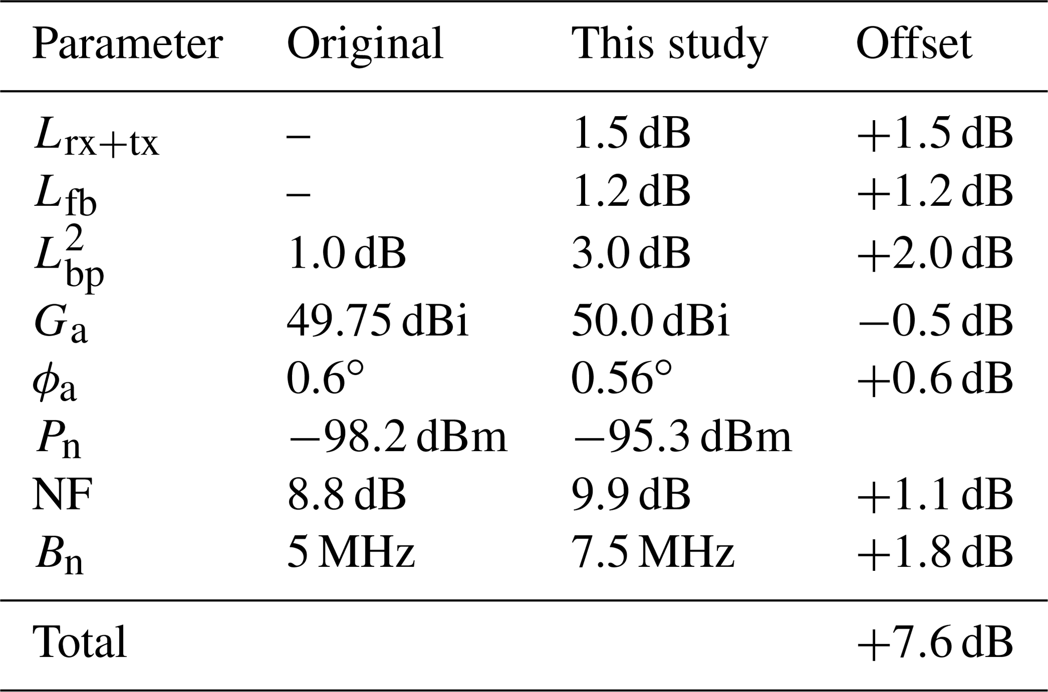
A key component of this work was the characterization of the spectral response and the transfer function of the receiver. In a wide dynamic range of 70 dB, the receiver response turned out to be very linear (residual 0.05 dB). Using different attenuator settings, it covers a wide input range from −105 to −5 dBm. This characterization gave valuable new insights into the receiver sensitivity and additional attenuations which led to a major improvement of the absolute calibration. The comparison of the measured and the previously estimated total receiver noise power (−95.3 vs. −98.2 dBm) revealed an underestimation of 2.9 dB. This underestimation could be traced back to a larger receiver noise bandwidth of 7.5 MHz (instead of 5 MHz) and a slightly higher noise figure (1.1 dB). Measurements confirmed the previously assumed antenna gain (50.0 dBi) with no obvious asymmetries or increased side lobes. The calibration used for previous campaigns, however, did not account for a 1.5 dB two-way attenuation by additional waveguides in the airplane installation. Laboratory measurements also revealed a 2 dB higher two-way attenuation by the belly pod caused by small deviations during manufacturing. In total, effective reflectivities measured during previous campaigns had to be corrected by +7.6 dB.
To validate this internal calibration, the well-defined ocean surface backscatter was used as a calibration reference. With the new absolute calibration, the ocean surface backscatter measured by HAMP MIRA agrees very well (<1 dB) with modeled values and values measured by the GPM satellite. As a further cross-check, flight experiments over Europe and the tropical North Atlantic were conducted. To that end, a joint flight of HALO and the French Falcon 20 aircraft, which was equipped with the RASTA cloud radar at 94 GHz and an underflight of the spaceborne CloudSat at 94 GHz were performed. The intercomparison revealed lower reflectivities (−1.4 dB) for RASTA but slightly higher reflectivities (+1.0 dB) for CloudSat. With effective reflectivities between RASTA and CloudSat and the good agreement with GPM, the accuracy of the absolute calibration is estimated to be around 1 dB.
- Article
(9380 KB) - Full-text XML
- BibTeX
- EndNote


In recent years, the deployment of cloud profiling microwave radars on the ground, on aircraft as well as on satellites, like CloudSat (Stephens et al., 2002) or the upcoming EarthCARE satellite mission (Illingworth et al., 2014), have greatly advanced our scientific knowledge of cloud microphysics. Nevertheless, large discrepancies in retrieved cloud microphysics (Zhao et al., 2012; Stubenrauch et al., 2013) contribute to uncertainties in the understanding of the role of clouds for the climate system (Boucher et al., 2013). An important aspect for enabling accurate microphysical retrievals based on cloud radar data is the proper calibration of the systems.
However, the absolute calibration of an airborne millimeter-wave cloud radar can be a challenging task. Its initial calibration demands detailed knowledge of cloud radar technology and the availability of suitable measurement devices. During cloud radar operation, system parameters of transmitter and receiver system can drift due to changing ambient temperature, pressure and aging system components. The validation of the absolute calibration with external sources is furthermore complicated for downward-looking installations on an aircraft. The missing ability of most airborne and many ground-based radars to point their line of sight to an external reference source makes it difficult or even completely impossible to calibrate the overall system with an external reference in a laboratory.
Typically, an budget approach is used for the absolute calibration of airborne cloud radar instruments. First, the instrument components like transmitter, receiver, waveguides, antenna and radome are characterized individually in the laboratory. During in-flight measurements, variable component parameters are then monitored and corrected for drifts using the laboratory characterization. Subsequently, all gains and losses are combined into an overall instrument calibration.
In order to meet the required absolute accuracy and to follow good scientific practice, an external in-flight calibration becomes indispensable to check the internal calibration for systematic errors. For weather radars, the well-defined reflectivity of calibration spheres on tethered balloons or erected trihedral corner reflectors has been a reliable external reference for years (Atlas, 2002). In more recent years, this technique is being extended to scanning, ground-based millimeter-wave radars (Vega et al., 2012; Chandrasekar et al., 2015). For the airborne perspective on the other hand, the direct fly-over and the subsequent removal of additional background clutter is difficult to reproduce (Z. Li et al., 2005).
Driven by this challenge, many studies have been conducted to characterize the characteristic reflectivity of the ocean surface using microwave scatterometer–radiometer systems in the X and Ka bands (Valenzuela, 1978; Masuko et al., 1986). As one of the first, Caylor (1994) introduced the ocean surface backscatter technique to cross-check the internal calibration of the NASA ER-2 Doppler radar (EDOP; Heymsfield et al., 1996). In an important next step, L. Li et al. (2005) combined this technique with analytical models of the ocean surface backscatter. In their work, they used circle and roll maneuvers to sample the ocean surface backscatter for different incidence angles with the Cloud Radar System (CRS; Li et al., 2004), a 94 GHz (W band) cloud radar on board the NASA ER-2 high-altitude aircraft. In this context, they proposed to point the instrument 10∘ off-nadir, an angle for which multiple studies found a very constant ocean surface backscatter (Durden et al., 1994; Z. Li et al., 2005; Tanelli et al., 2006). For this incidence angle, these studies confirmed the ocean surface to be relatively insensitive to changes in wind speed and wind direction.
Subsequent studies followed suit, applying the same technique to other airborne cloud radar instruments: the Japanese W-band Super Polarimetric Ice Crystal Detection and Explication Radar (SPIDER; Horie et al., 2000) on board the NICT Gulfstream II by Horie et al. (2004), the Ku/Ka-band Airborne Second Generation Precipitation Radar (APR-2; Sadowy et al., 2003) on board the NASA P-3 aircraft by Tanelli et al. (2006) and the W-band cloud radar (RASTA; Protat et al., 2004) on board the SAFIRE Falcon 20 by Bouniol et al. (2008).
Encouraged by these airborne studies, this in-flight calibration technique has also been proposed and successfully applied to the spaceborne CloudSat instrument (Stephens et al., 2002; Tanelli et al., 2008). Based on this success, Horie and Takahashi (2010) proposed the same technique with a whole 10∘ across-track sweep for the next spaceborne cloud radar, the 94 GHz Doppler Cloud Profiling Radar (CPR) on board EarthCARE (Illingworth et al., 2014).
With CloudSat as a long-term cloud radar in space, direct comparisons of radar reflectivity from ground- and airborne instruments became possible (Bouniol et al., 2008; Protat et al., 2009). While the first studies still assessed the stability of the spaceborne instrument, subsequent studies turned this around by using CloudSat as a Global Radar Calibrator for ground-based or airborne radars Protat et al. (2010).
This work will focus on the internal and external calibration of the MIRA cloud radar (Mech et al., 2014) on board the German High Altitude and Long Range Research Aircraft (HALO), adopting the ocean surface backscattering technique described by Z. Li et al. (2005). In the first part, the preflight laboratory characterization of each system component will be described. This includes antenna gain, component attenuation and receiver sensitivity. In a budget approach, these system parameters are then used in combination with in-flight monitored transmission and receiver noise power levels to form the internal calibration. The second part will then compare the internal calibration with external reference sources in-flight. As external reference sources, measurements of the ocean surface as well as intercomparisons with other air- and spaceborne cloud radar instruments will be used.
This paper is organized as follows: after some considerations about required radar accuracies shown in Sect. 1, Sect. 2 introduces the cloud radar instrument and its specifications on board the HALO research aircraft. Section 3 recalls the radar equation and introduces the concept of using the ocean surface backscatter for radar calibration. The characterization and calibration of the single system components, including waveguides, antenna and belly pod, is described in Sect. 3.1. Subsequently, the overall calibration of the radar receiver is explained in Sect. 3.2. Here, a central innovation of this work is the determination of the receiver sensitivity (Sect. 3.3 and 3.4). In the second part of the paper, the budget calibration is validated by using predicted and measured ocean surface backscatter (Sect. 4.3). In addition, the calibration and system performance for joint flight legs is compared to the W-band cloud radars like the airborne cloud radar RASTA (Sect. 5.2) and the spaceborne cloud radar CloudSat (Sect. 5.3).
Accuracy considerations
In order to provide scientifically sound interpretations of cloud radar measurements, a well-calibrated instrument with known sensitivity is indispensable. Many spaceborne (Delanoë and Hogan, 2008; Deng et al., 2010) or ground-based (Donovan et al., 2000) techniques to retrieve cloud microphysics using millimeter-wave radar measurements require a well-calibrated instrument. In the case of the CloudSat instrument, the calibration uncertainty was specified to be ±2 dB or better (Stephens et al., 2002). This requirement for absolute calibration imposed by retrievals of cloud microphysics is further explained in Fig. 1. Under the simplest assumption of small, mono-disperse cloud water droplets, the iso-lines in Fig. 1 represent all combinations of cloud droplet effective radius and liquid water content with a radar reflectivity of −20 dBz. An increasing retrieval ambiguity, caused by an assumed instrument calibration uncertainty, is illustrated by the shaded areas with ±1 dB (green), ±3 dB (yellow) and ±8 dB (red). To constrain the retrieval space considerably within synergistic radar–lidar retrievals like Cloudnet (Illingworth et al., 2007) or Varcloud (Delanoë and Hogan, 2008), the absolute calibration uncertainty has to be significantly smaller than the natural variability of clouds. Since a reflectivity bias of 8 dB would bias the droplet size by a factor of 2 and the water content by even an order of magnitude, the absolute calibration uncertainty should be at least 3 dB or lower. For a systematic 1 dB calibration offset, Protat et al. (2016) still found ice water content biases of +19 % and −16 % in their radar-only retrieval. Since HAMP MIRA data are used in retrievals of cloud microphysics, the target accuracy will be set to 1 dB.

Figure 1Microphysical retrieval uncertainty due to different absolute calibration uncertainties (±1, ±3, ±8) for mono-disperse cloud water droplets according to Mie calculations.
An accurate absolute calibration is further motivated by recent studies (Protat et al., 2009; Hennemuth et al., 2008; Maahn and Kollias, 2012; Ewald et al., 2015; Lonitz et al., 2015; Myagkov et al., 2016; Acquistapace et al., 2017), which used the radar reflectivity provided by almost identical ground-based versions of the same instrument. The installation of the MIRA instrument on many ground-based cloud profiling sites within ACTRIS (Aerosols, Clouds and Trace gases Research InfraStructure Network; http://www.actris.eu, last access: 10 March 2019) and in the framework of Cloudnet is a further incentive for an external calibration study.
The need for an external calibration is furthermore encouraged by several studies which already found evidence of an offset in radar reflectivity when comparing different cloud radar instruments. In a direct comparison with the W-Band (94 GHz) ARM Cloud Radar (WACR), Handwerker and Miller (2008) found reflectivities around 3 dB smaller for the Karlsruhe Institute of Technology MIRA, contradicting the reflectivity-reducing effect of a higher gaseous attenuation and stronger Mie scattering at 94 GHz. Protat et al. (2009) could reproduce this discrepancy in a comparison with CloudSat, where they found a clear systematic shift of the mean vertical profile by 2 dB between Cloudsat and the Lindenberg MIRA (CloudSat showing higher values than the Lindenberg radar).
The cloud radar on HALO is a pulsed Ka-band, polarimetric Doppler millimeter-wavelength radar which is based on prototypes developed and described by Bormotov et al. (2000) and Vavriv et al. (2004). The current system was manufactured and provided by Metek (Meteorologische Messtechnik GmbH, Elmshorn, Germany). The system design and its data processing, including an updated moment estimation and a target classification by Bauer-Pfundstein and Görsdorf (2007), was described in detail by Görsdorf et al. (2015). The millimeter radar is part of the HALO Microwave Package (HAMP) which will be subsequently abbreviated as HAMP MIRA. Its standard installation in the belly pod section of HALO with its fixed nadir-pointing 1 m diameter Cassegrain antenna is described in detail by Mech et al. (2014). Its transmitter is a high-power magnetron operating at 35.5 GHz with a peak power Pt of 27 kW, with a pulse repetition frequency fp between 5 and 10 kHz and a pulse width τp between 100 and 400 ns. The large antenna and the high peak power can yield an exceptionally good sensitivity of −47 dBZ for the ground-based operation (5 km distance, 1 s averaging and a range resolution of 30 m). In the current airborne configuration, the sensitivity is reduced to −39.8 dBZ by various circumstances which will be addressed in this paper. The broadening of the Doppler spectrum due to the beam width can reduce this sensitivity further by 9 dB, as discussed in Mech et al. (2014). Table 1 lists the technical specifications as characterized in this work. Boldface indicates the operational configuration.
Table 1Technical specifications of the HAMP cloud radar as characterized in this work. Boldface indicates the operational configuration used in this work.
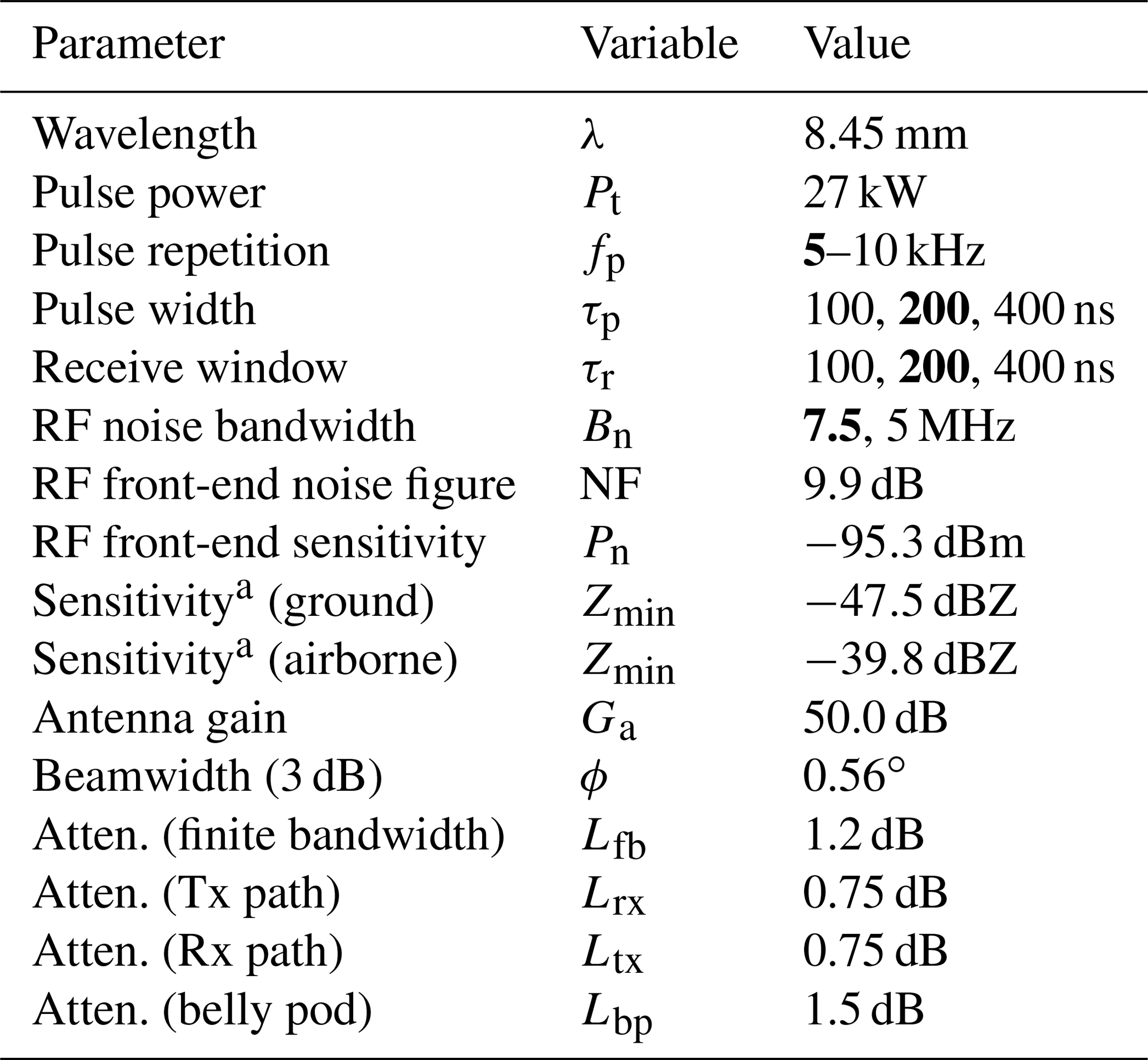
a At 5 km, 1 s average, 30 m resolution.
Most of the parameters in Table 1 play a role in the absolute calibration of the cloud radar instrument. For this reason, this section will briefly recapitulate the conversion from receiver signal power to the commonly used equivalent radar reflectivity factor Ze. When the radar reflectivity η of a target is known, e.g., in modeling studies, its equivalent radar reflectivity factor is given by
where |K|2=0.93 is the dielectric factor for water and λ the radar wavelength. For brevity, the equivalent radar reflectivity factor Ze is referred to as “effective reflectivity” in this paper. Following the derivation of the meteorological form of the radar equation by Doviak and Zrnić (2006), the effective reflectivity Ze (mm6 m−3) can be calculated from the received signal power Pr (W) by
where r is the range between antenna and target, Latm is the one-way path integrated attenuation, and Rc is a constant which describes all relevant system parameters. Assuming a circularly symmetric Gaussian antenna pattern, this radar constant Rc contains the pulse wavelength λ (m), pulse width τp (s) and peak transmit power Pt in milliwatts, the peak antenna gain Ga, and the antenna half-power beamwidth ϕ. Additionally, it accounts for all attenuations Lsys occurring in system components, e.g., in transmitter (Ltx) and receiver (Lrx) waveguides, due to the belly pod radome and due to the finite receiver bandwidth (Lfb):
Usually, antenna parameters (Ga,ϕ) and system losses () have to be determined only once for each system modification. In contrast, transmitter and receiver parameters have to be monitored continuously. In addition, a thorough characterization of the receiver sensitivity is essential for the absolute accuracy of the instrument.
This section will discuss the internal calibration of the radar instrument and its characterization in the laboratory. The following section will then compare this budget approach in-flight with an external reference source.
The monitoring of the system-specific parameters and the subsequent estimation of effective reflectivity are described in detail by Görsdorf et al. (2015). The internal calibration (budget calibration) strategy for HAMP MIRA is therefore only briefly summarized here. In case of a deviation, previously assumed and used parameters will be given and referred to as initial calibration for traceability of past radar measurements.
3.1 Antenna, radome and waveguides
-
Antenna. The gain Ga=50.0 dBi and the beam pattern (−3 dB beamwidth ϕ=0.56∘) was determined by the manufacturer following the procedure described by Myagkov et al. (2015). Hereby the 1 m diameter Cassegrain antenna was installed on a pedestal to scan its pattern on a tower 400 m away. The antenna pattern showed no obvious asymmetries or increased side lobes (side lobe level: −22 dB). Its characterization revealed no significant differences in comparison with the initially estimated parameters (Ga=49.75 dBi, ϕ=0.6∘).
-
Radome. The thickness of the epoxy quartz radome in the belly pod was designed with a thickness of 4.53 mm to limit the one-way attenuation to around 0.5 dB. Deviations during manufacturing increased the thickness to 4.84 mm, with a one-way attenuation of around 1.5 dB. Laboratory measurements confirmed this 2.0 dB (2×1.0 dB) higher two-way attenuation compared to the initially used value for the radome attenuation. A detailed analysis of this deviation can be found in Appendix B.
-
Waveguides. The initially used calibration did not account for the losses caused by the longer waveguides in the airplane installation. Actually, transmitter and receiver waveguides each have a length of 1.15 m. With a specified attenuation of 0.65 dB m−1, the two-way attenuation by waveguides is thus 1.5 dB.
3.2 Transmitted and received signal power
-
Transmitter peak power Pt. Due to strong variations in ambient temperatures in the cabin, in-flight thermistor measurements proved to be unreliable. For this reason, thermally controlled measurements of Pt were conducted on the ground, which were correlated with measured magnetron currents Im. The relationship between both parameters then allowed Pt to be derived from in-flight measurements of Im. A detailed analysis of this relationship can be found in Appendix A.
-
Finite receiver bandwidth loss Lfb. The loss caused by a finite receiver bandwidth was discussed in detail by Doviak and Zrnić (1979). For a Gaussian receiver response, the finite receiver bandwidth loss Lfb can be estimated using
Here, B6 is the 6 dB filter bandwidth of the receiver and τp is the duration of the pulse. During the initial calibration, no correction of the finite receiver bandwidth loss was applied.
-
Signal-to-noise ratio (SNR). For each sampled range, MIRA's digital receiver converts phase shifts of consecutive pulse trains (e.g., NP=256 pulses) into power spectra of Doppler velocities vi by a real-time fast Fourier transform (FFT). First, spectral densities sj(vi) of multiple power spectra are averaged (e.g., NS=20 spectra) to enhance the signal-to-noise ratio. Subsequently, the averaged spectral densities in individual velocity bins are summed to yield a total received signal S in each gate:
The receiver chain omits a separate absolute power meter circuit. At the end of each pulse cycle, the receiver is switched to internal reference gates by a pin diode in front of the first amplifier. These two last gates are called the receiver noise gate and the calibration gate. To obtain the received backscattered signal Sr in atmospheric gates, one has to subtract the signal received in the noise gate Sng from the total received signal S since it contains both signal and noise:
In that way, a signal-to-noise ratio is then calculated by dividing the received backscattered signal Sr in each atmospheric gate by the signal Sng measured in the noise gate:
The relative power of the calibration gate to the receiver noise gate is furthermore used to monitor the receiver sensitivity (for details see Sect. 3.3). The main advantage of this method is the simultaneous monitoring of the relative receiver sensitivity using the same circuitry that is used for atmospheric measurements. Furthermore, the determination of the receiver noise in a separate noise gate can prevent biases in SNR, when the noise floor in atmospheric gates is obscured by aircraft motion or strong signals, both leading to a broadened Doppler spectrum.
Following Riddle et al. (2012), the minimum SNRmin can be calculated in terms of NP and NS, if the backscattered signal power is contained in a single Doppler velocity bin:
Here, Q=7 is a threshold factor between the received signal and the standard deviation of the noise signal. In the absence of any turbulence- or motion-induced Doppler shift, the operational configuration yields a SNRmin of −22.1 dB. As discussed in Mech et al. (2014), this minimum SNR can be larger by 9 dB due to a motion-induced broadening of the Doppler spectrum in the airborne configuration.
-
Received signal power Pr. The SNR response of the receiver to an input power Pr is described by a receiver transfer function SNR=𝒯(Pr). When 𝒯 is known, an unknown received signal power Pr can be derived from a measured SNR by the inversion 𝒯−1:
-
Receiver sensitivity Pn. For a linear receiver, 𝒯−1 can be approximated by a signal-independent receiver sensitivity Pn, which translates a measured SNR to an absolute signal power Pr in dBm:
More specifically, Pn can be interpreted as an overall receiver noise power and is thus equal to the power of the smallest measurable white signal. It includes the inherent thermal noise within the receiver response, the overall noise figure of the receiver and mixer circuitry and all losses occurring between ADC and receiver input.
3.3 Estimated receiver sensitivity
Prior to this work, no rigorous determination of the receiver transfer function 𝒯 was performed. During the initial calibration, the receiver sensitivity Pn was instead estimated using the inherent thermal noise and its own noise characteristic.
Generated by thermal electrons, the inherent thermal noise PkTB received by a matched receiver can be derived using Boltzmann's constant kB, temperature T0 and the noise bandwidth Bn of the receiver. Additional noise power is introduced by the electronic circuitry itself, which is considered by the receiver noise factor Fn. The noise factor Fn expressed in decibels (dB) is called noise figure NF. Combined, PkTB and Fn yield the total inherent noise power :
Using a calibrated external noise source with known excess noise ratio (ENR), Fn was determined in the laboratory. In-flight, Fn is monitored using the calibration and the noise gate.
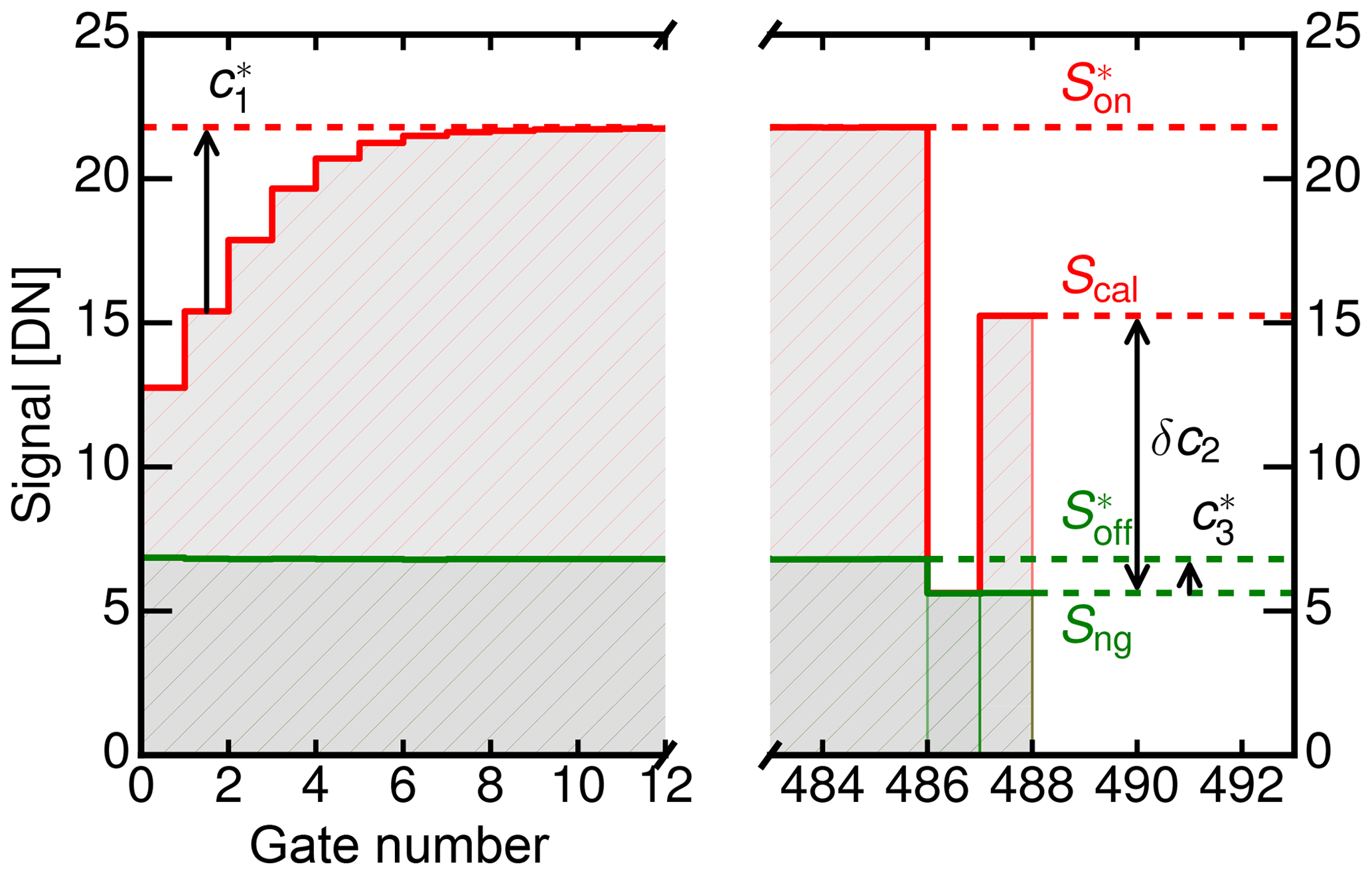
Figure 2Total received signal S in digital numbers as a function of gate number with external noise source switched on (, red) and switched off (, green). The two last gates monitor the signals Sng and Scal, which correspond to the receiver noise and the internal calibration source. The factors , c2 and correct the estimated noise power to reflect the actual receiver sensitivity Pn. Signal levels obtained only during the calibration with the external noise source are marked with an asterisk.
In the following, measurements obtained with the calibrated external noise source in the laboratory are marked with an asterisk. Signal levels measured in-flight as well as during the calibration are marked without an asterisk. Figure 2 shows the external noise source measurements, where the received signal S is plotted as a function of the gate number. While connected to the receiver input, the external noise source is switched on and off with signals (red) and (green) measured in atmospheric gates. Corresponding to this, and are the signals measured in the two last gates, namely the calibration and the receiver noise gates. The in-flight signals in these two reference gates are denoted by Scal and Sng.
Using the so called Y-factor method (Agilent Technologies, 2004), the averaged noise floor ratio Y in atmospheric gates between the external noise source being switched on and off and the ENR of the external noise source is used to determine the noise factor Fn created by the receiver components:
Here, the averaging of atmospheric gates is done for gate numbers larger than 10 to exclude the attenuation caused by the transmit–receive switch immediately after the magnetron pulse. During the initial calibration with the external noise source, a noise figure NF=8.8 dB was determined.
Summarizing the above considerations, an overall receiver sensitivity is estimated using an assumed receiver noise bandwidth of 5 MHz, a receiver temperature of 290 K and a noise figure of NF=8.8 dB. According to Eq. (12), the estimated receiver sensitivity used in the initial calibration is
The measurements with the external noise source are furthermore exploited to correct for various effects, which cause deviations between the inherent noise power in the noise gate and the actual receiver sensitivity Pn:
Here, the following applies:
-
accounts for the attenuation in atmospheric gates, which is caused by the transmit–receive switch immediately after the magnetron pulse:
As evident in Fig. 2, is only significant in the first eight range gates (=240 m) and rapidly converges to 0 dB in the remaining atmospheric and reference gates.
-
Secondly, the correction factor c2 is used to monitor and correct in-flight drifts of the receiver sensitivity. To this end, the ratio measured during calibration between calibration and noise gate is compared to the ratio Scal∕Sng during flight:
In the course of one flight of several hours, c2 varies only slightly by ±0.5 dB. Continuous observation of c2 should be performed to keep track of the receiver sensitivity.
-
A further factor accounts for the fact that the noise level measured in the noise gate is lower than the total system noise with matched load because the low-noise amplifier is not matched during the noise gate measurement. The SNR† determined with the noise gate level therefore overestimates the actual SNR in atmospheric gates:
In Fig. 2, this offset is called . Its value is determined by comparing the signal in the noise gate with the signal in atmospheric gates, while the external noise source is switched off:
This offset between noise gate and total system noise remains very stable with dB. Since exists only in earlier MIRA-35 systems (without MicroBlaze processor, e.g. KIT, UFS, HALO and Lindenberg), most MIRA-35 operators do not have to address this issue.
3.4 Measured receiver sensitivity
A key component of this work was to replace the estimated receiver sensitivity with an actual measured value Pn. While was calculated using an assumed receiver noise bandwidth and the receiver noise factor, Pn is now measured directly using a calibrated signal generator with adjustable power and frequency output. By varying the power at the receiver input, Pn is found as the noise-equivalent signal when SNR=0 dB. In addition, the receiver response and its bandwidth is determined by varying the frequency of the signal generator. Both measurements are then used to evaluate and check Fn according to Eq. (12). This is done for two different matched filter lengths (τr=100 ns, τr=200 ns) to characterize the dependence of Bn and Fn on τr.
To this end, an analog continuous wave signal generator E8257D from Agilent Technologies was used to determine the receiver's spectral response and its power transfer function 𝒯. The signal generator was connected to the antenna port of the radar receiver and tuned to 35.5 GHz, the central frequency of the local oscillator. For the characterization, the radar receiver was set into standard airborne operation mode. In this mode, 256 samples are averaged coherently into power spectra by FFT. Subsequently, 20 power spectra are then averaged to obtain a smoothed power spectrum for each second.
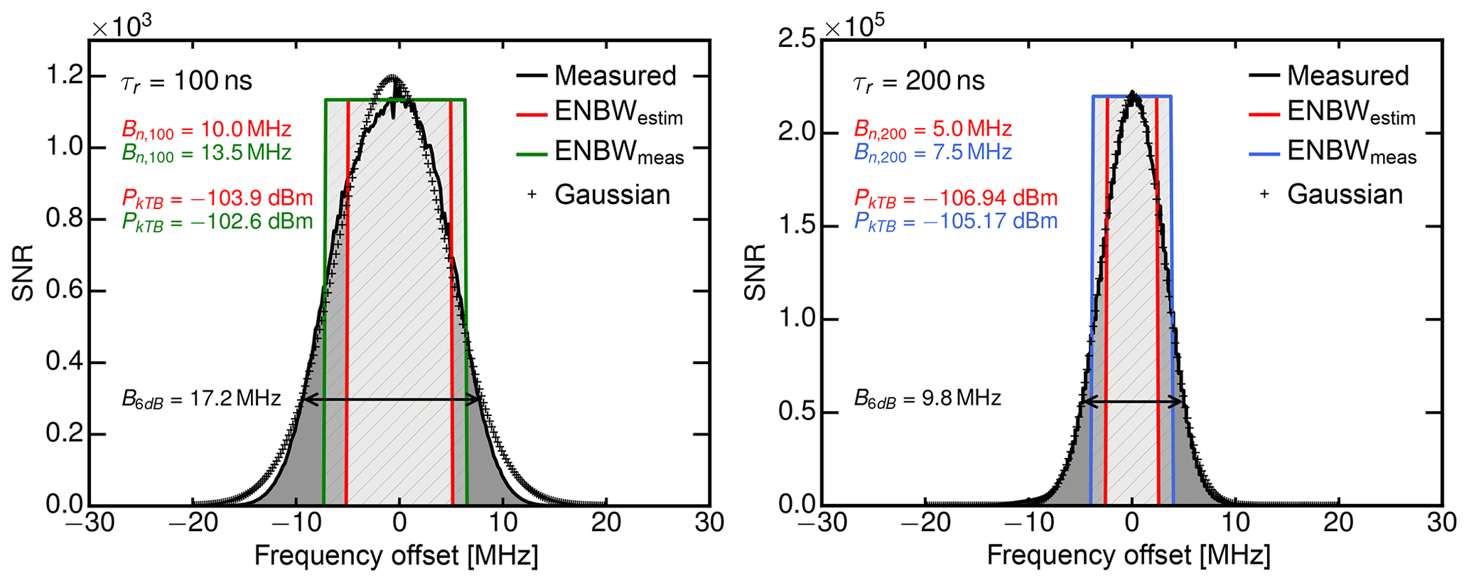
Figure 3Measured radar receiver response (gray) as a function of the frequency offset from the center frequency at 35.5 GHz for two different matched filter lengths. While the green and blue hatched rectangles show the actual equivalent noise bandwidths, the red-hatched rectangles show the estimated noise bandwidth that was used in the initial calibration.
3.4.1 Receiver bandwidth
To determine the spectral response, the frequency sweep mode of the signal generator with a fixed signal amplitude was used within a region of 35 500±20 MHz. For the shorter match filter length (τr=100 ns) on the left and for the longer matched filter length (τr=200 ns) on the right, Fig. 3 shows measured signal-to-noise ratios as a function of the frequency offset from the center frequency at 35.5 GHz. The spectral response of the receiver for both matched filters (black lines) approaches a Gaussian fit (crosses). To estimate the finite receiver bandwidth loss Lfb using Eq. (4), the 6 dB filter bandwidth (two-sided arrow) is determined directly from the receiver response with B6=9.8 MHz for τr=200 ns and B6=17.2 MHz for τr=100 ns. In the following, the equivalent noise bandwidth (ENBW) concept is used to determine the receiver noise bandwidth Bn which is needed to calculate Pn. In short, the ENBW is the bandwidth of a rectangular filter with the same received power as the actual receiver. Illustrated by the green and blue hatched rectangles in Fig. 3, the measured ENBW is MHz for the longer matched filter length and MHz for the shorter matched filter length. In contrast, the red-hatched rectangles show the estimated 5 MHz (and 10 MHz) receiver noise bandwidth using 1∕τr. The discrepancy between the measured and the estimated noise bandwidth could be traced back to an additional window function which was applied unintentionally to IQ data within the digital signal processor. This issue led to a bit more thermal noise power PkTB. For the operationally used matched filter (τr=200 ns), the offset between estimated and actual thermal noise power (−106.9 vs. −105.2 dBm) led to an 1.8 dB underestimation of Ze. Future measurements will not include this bias since this issue was found and fixed.
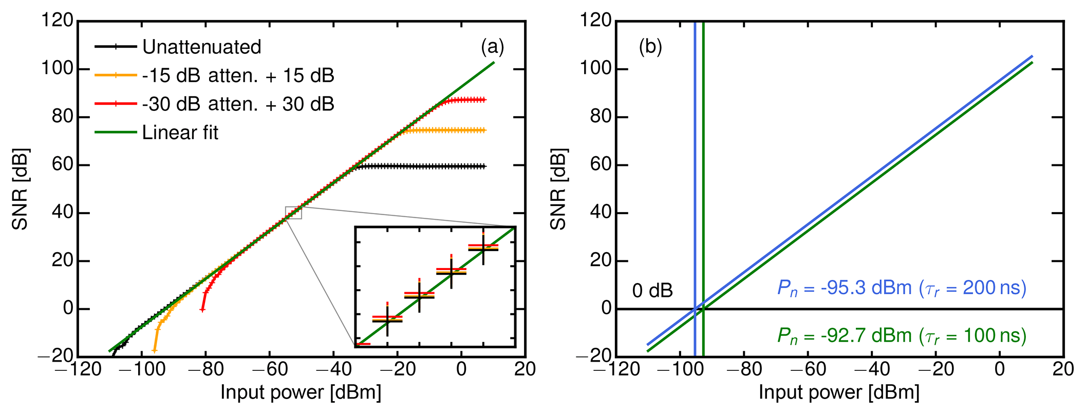
Figure 4(a) Measured receiver transfer functions for the three attenuator settings of 0 dB (black), 15 dB (green) and 30 dB (red). (b) Linear regression receiver transfer function to determine the receiver sensitivity Pn.
3.4.2 Receiver transfer function
Next, the amplitude ramp mode of the signal generator was used to determine the transfer function Pr=𝒯(SNR) of the receiver. The receiver transfer function references absolute signal powers at the antenna port with corresponding SNR values measured by the receiver. Moreover, the linearity and cut-offs of the receiver can be assessed on the basis of the transfer function. For this measurement, the frequency of the signal generator was set to 35.5 GHz, while the output power of the generator was increased steadily from −110 to 10 dBm. This was done in steps of 1 dBm while averaging over 10 power spectra. In order to test the linearity and the saturation behavior of the receiver for strong signals, these measurements were repeated with an internal attenuator set to 15 and 30 dB. For τr=200 ns, Fig. 4a shows the measured receiver transfer functions for the three attenuator settings of 0 dB (black), 15 dB (green) and 30 dB (red). For measurements with an activated attenuator, SNR values have been corrected by +15 dB (respectively +30 dB) to compare the transfer functions to the one with 0 dB attenuation. The overlap of the different transfer functions between input powers of −70 and −30 dBm in Fig. 4a confirms the specified attenuator values of 15 and 30 dB. Furthermore, no further saturation by additional receiver components (e.g., mixers or filters) can be detected up to an input power of −5 dBm. This allows the dynamic range to be shifted by using the attenuator to measure higher input powers (which would otherwise be saturated) without losing the absolute calibration. This feature is essential for the evaluation of very strong signals like the ground return.
Subsequently, a linear regression to the results without an attenuator was performed between input powers of −70 and −40 dBm, which is shown in Fig. 4b.
With a slope m of 1.0009 (±0.0006) and a residual of 0.054 dB, the receiver behaved very linearly for this input power region. Similar values were obtained for an attenuation of +15 dB with a slope of 0.9980 (±0.0005) and a residual of 0.024 dB and a slope of 0.9884 (±0.0013) and a residual of 0.1 dB for an attenuation of +30 dB.
3.4.3 Receiver sensitivity
Finally, the linear regression to the receiver transfer function can be used to derive the receiver sensitivity Pn. Its x-intercept (SNR=0) directly yields the receiver sensitivity Pn for the two matched filter lengths:
As discussed before, the setting with the shorter matched filter length collects more thermal noise due to the larger receiver bandwidth. In a final step, this top-down approach to obtain Pn for different τr can be used to determine Fn and check for its dependence on τr. By solving Eq. (12) for Fn and inserting the measured bandwidths B100 and B200 we obtain the following:
Remarkably, Fn shows no dependence on τr but turns out to be larger than previously estimated by 1.1 dB. This previous underestimation of Fn led to an 1.1 dB underestimation of Ze.
Now, all system parameters are known to estimate the radar sensitivity at a particular range. Following Doviak and Zrnić (2006), the minimum detectable effective reflectivity Zmin(r) at a particular range can be calculated using Eq. (2) in decibels:
Here, Pr is the minimum detectable signal (MDS) in dBm which is given by Pn SNRmin using Eq. (11):
In the operational configuration (Q=7, NP=256, NS=20), the MDS is −117.4 dBm, since dB and dBm. The parameters listed in Table 1 yield a range-independent radar constant of Rc=3.9 dB. Using the MDS and Rc in Eq. (26), the minimum detectable effective reflectivity in 5 km is dBZ.
3.5 Overall calibration budget
Comparing the measured dBm to the estimated dBm for τr=200 ns, the combination of bandwidth bias (1.8 dB) and larger noise figure (1.1 dB) caused a 2.9 dB underestimation of Ze. Combined with the disregard of the 2.0 dB higher two-way attenuation by the radome and the 1.5 dB higher two-way attenuation by the waveguides as well as the disregard of the finite receiver bandwidth loss Lfb of 1.2 dB, effective reflectivities derived with the initial calibration has to be corrected by +7.6 dB. Table 2 summarizes and breaks down all offsets found in this work.
Table 2Breakdown of the offset between original and new calibration for each system parameter. Values for Lrx+tx and Lfb were already known but not applied in past measurement campaigns. The total offset has to be applied to Rc and Ze.
The following section will now test the absolute calibration using an external reference target. As already mentioned in the introduction, the ocean surface has been used as a calibration standard for air- and spaceborne radar instruments. In their studies, Barrick et al. (1974) and Valenzuela (1978) reviewed and harmonized theories to describe the interaction of electro-magnetic waves with the ocean surface. They showed that the normalized radar cross section σ0 of the ocean surface at small incidence angles (Θ<15∘) can be described by quasi-specular scattering theory. At larger incidence angles (Θ>15∘), Bragg scattering at capillary waves becomes dominant, which complicates and enhances the backscattering of microwaves by ocean waves.
4.1 Modeling the normalized radar cross section of the ocean surface
At the scales of millimeter waves and for small incidence angles θ, the ocean surface slope distribution is assumed to be Gaussian and isotropic, where the surface mean square slope s(v) is a sole function of the wind speed v and independent from wind direction. Backscattered by ocean surface facets, which are aligned normal to the incidence waves (Plant, 2002), the normalized radar cross section σ0 can be described as a function of ocean surface wind speed v and beam incidence angle θ (Valenzuela, 1978; Brown, 1990; Z. Li et al., 2005):
For the ocean surface facets at normal incidence, the reflection of microwaves is described by an effective Fresnel reflection coefficient . In this study, the complex refractive index for seawater at 25 ∘C is used following the model by Klein and Swift (1977). Like with other models (Ray, 1972; Meissner and Wentz, 2004), the impact of salinity on σ0 is negligible, while the influence of the ocean surface temperature on σ0 stays below Δσ0=0.5 dB between 5 and 30 ∘C. Since specular reflection is only valid in the absence of surface roughness, various studies (Wu, 1990; Jackson et al., 1992; Freilich and Vanhoff, 2003; L. Li et al., 2005) included a correction factor Ce to describe the reflection of microwaves on wind-roughened water facets. While Ce has been well characterized for the Ku band (Apel, 1994; Freilich and Vanhoff, 2003) and W band (Horie et al., 2004; L. Li et al., 2005), experimental results valid for the Ka band are scarce (Nouguier et al., 2016). Tanelli et al. (2006) used simultaneous measurements of σ0 in the Ku and Ka bands, to determine for the Ka band, which corresponds to an correction factor Ce of 0.90. However, there is an ongoing discussion about the influence of radar wavelength or wind speed on Ce (Jackson et al., 1992; Tanelli et al., 2008). Chen et al. (2000) explains this disagreement with the different surface mean square slope statistics used in these studies, which do not include ocean surface roughness at the millimeter scale. To include this uncertainty in this study, the correction factor Ce has been varied between 0.85 and 0.95, while the simple model (CM) for non-slick ocean surfaces by Cox and Munk (1954) was used for s(v). In their model, the surface mean square slope s(v) scales linearly with wind speed v, describing a smooth ocean surface including gravity and capillary waves:
4.2 Measuring the normalized radar cross section of the ocean surface
The ocean surface backscatter is also measured by the Global Precipitation Measurement (GPM; Hou et al., 2013) platform which carries a Ku- and Ka-band dual-frequency precipitation radar (DPR). For this study, from GPM is used as an independent source to support the calculated σ0 from the model. Operating at 35.5 GHz, the KaPR scans the surface backscatter with its 0.7∘ beamwidth phased array antenna, resulting in a 120 km swath of 5 km×5 km footprints. The measured ocean surface backscatter by GPM is operationally used to retrieve surface wind conditions and path-integrated attenuation of the radar beam. In the following, the corrected for gaseous attenuation from GPM was used, which corresponds to the co-localized matched swath of the KaPR.
During the second Next-Generation Remote Sensing for Validation Studies (NARVAL2) in June–August 2016, HAMP MIRA was deployed on HALO. The campaign was focused on the remote sensing of organized convection over the tropical North Atlantic Ocean in the vicinity of Barbados. Another campaign objective was the integration and validation of the new remote sensing instruments on board the HALO aircraft. For the HAMP MIRA cloud radar, multiple roll and circle maneuvers at different incidence angles were included in research flights to implement the well-established calibration technique to measure the normalized radar cross section of the ocean surface at different incidence angles.
During NARVAL2, HAMP MIRA was installed in the belly pod section of HALO and aligned in a fixed nadir-pointing configuration with respect to the airframe. The incidence angle is therefore controlled by pitch-and-roll maneuvers of the aircraft. The aircraft position and attitude are provided at a 10 Hz rate by the BAsic HALO Measurement And Sensor System (BAHAMAS; Krautstrunk and Giez, 2012). Pitch, roll and yaw angles are provided with an accuracy of 0.05∘, while the absolute uncertainty can be up to 0.1∘. Additional incidence angle uncertainty is caused by uncertainties in the alignment of the radar antenna. Following the approach of Haimov and Rodi (2013), the apparent Doppler velocity of the ground was used to determine the antenna beam-pointing vector. With this technique, the offsets from nadir with respect to the airframe was determined with 0.5∘ to the left in the roll direction and 0.05∘ forward in the pitch direction.
During calibration patterns, HALO flew at 9.7 km altitude with a ground speed of 180 to 200 ms−1. The pulse repetition frequency was kept at 6 kHz with a pulse length of τp=200 ns. For the purpose of calibration, the data processing and averaging was set to 1 Hz, being the standard campaign setting with Doppler spectra averaged from 20 FFTs, which each contain 256 pulses. As a consequence of this configuration, the ocean surface backscatter at nadir was sampled in gates measuring approx. 100 m in the horizontal and 30 m in the vertical. With this gate geometry, a uniform beam-filling of the ocean surface is ensured for incidence angles below 20∘.
In the current configuration, the point target spread function of the matched receiver is under-sampled since the sampling is matched to the gate length. Thus, the maximum of the ocean backscatter can become underestimated when the surface is located between two gates. At nadir incidence, negative bias values of σ0 of up to 3–4 dB were observed in earlier measurement campaigns, when the gate spacing equals or is larger than the pulse length (Caylor et al., 1997). For this reason, the received power from the range gates below and above were added to the received power of the strongest surface echo. By adding the power from only three gates, Caylor et al. (1997) could reduce the uncertainty in σ0 to 1 dB and exclude the contribution by antenna side-lobes from larger ranges.
Furthermore, the backscattered signal was corrected for gaseous attenuation by oxygen and water vapor considered in the loss factor Latm. While the two-way attenuation by oxygen and water vapor is normally almost negligible in the Ka band, it has to be considered in subtropical regions with high humidity and temperature near the surface. To this end, the gaseous absorption model for millimeter waves by Rosenkranz (1998) was used. Sounding profiles of pressure, temperature and humidity were provided by Vaisala RD-94 dropsondes, which were launched from HALO during the calibration maneuvers.
Following L. Li et al. (2005), the measured normalized cross section of the ocean surface can be calculated from measured signal-to-noise ratios:
Here, the receiver power Pr was replaced with PnSNR (Eq. 10) to include the overall receiver sensitivity Pn in the formulation of . Like in Eq. (2), Rc is the radar constant (with |K|2=1) which includes the transmitter power Pt, transmitting and receiving waveguide loss Ltx and Lrx, attenuation by the belly pod Lbp and the antenna gain Ga. Together with Pn, the combination of these system parameters are being checked in the following section, when the measured is compared to the modeled σ0. For the following analysis, was obtained with Eq. (30) using 1 Hz averaged SNR from HAMP MIRA.

4.3 Comparison of measurements and model
The HAMP MIRA calibration maneuver during NARVAL2 was included in research flight RF03 on 12 August 2016. The flight took place 700 km east of Barbados in a region of a relatively pronounced dry intrusion with light winds and very little cloudiness. Figure 5 shows the flight track in orange with a true-color image taken during that time by the geostationary SEVIRI instrument. The superimposed color map shows from GPM in the vicinity of the operating area for that day. Here, the satellite nadir is located in the center of each track, with inclination angles θ>0 left and right towards the edges of the swath. Apparently, seems spatially quite homogeneous, where the ocean surface is only covered by small marine cumulus clouds. The first way-point was chosen to be collocated with a meteorological buoy (14.559∘ N, 53.073∘ W, NDBC 41040) to obtain the accurate wind-speed and direction at the level of the ocean surface as well as wave heights measured by the buoy. At 12:50 UTC, the buoy measured a wind speed of 5.7 m s−1 from 98∘ with a mean wave height of 1 m and mean wave direction of 69∘. A detailed overview of the flight path during the calibration maneuver is shown in Fig. 6, where the beam incidence angle θ is shown by the color map. At 12:40 UTC, the aircraft executed a set of ±20∘ roll maneuvers to sample in the cross-wind direction. At 12:44 UTC, the aircraft entered a right-hand turn with a constant roll angle of 10∘, the incidence angle for which becomes insensitive to surface wind conditions and models. After a full turn at 12:58 UTC, another set of ±20∘ roll maneuvers were executed to sample in the along-wind direction. The dropsonde was launched around 13:06 UTC at 12.98∘ N and 52.78∘ W. A two-way attenuation by water vapor and oxygen absorption of 0.78 dB was calculated using the dropsonde sounding. With an approximate distance of 700 km, the GPM measurement closest to the calibration area was made at 10:46:29 UTC at 13.67∘ N and 59.53∘ W. To obtain a representative measurement from GPM, the swath data were averaged along-track for 10 s.

Figure 6Overview of the flight path during the calibration maneuver with the beam incidence angle θ shown by the color map.

Figure 7Normalized radar cross section (RCS) of the ocean surface as a function of the radar beam incident angle θ. (a) Falloff of with θ measured with HAMP MIRA (red/green dots) and GPM (blue circles). The HAMP MIRA data are calculated and subsequently fitted using the old, estimated calibration (red line) and the new, measured calibration (green line). The modeled value (CM: Cox–Munk) and uncertainty of σ0 for the actual measured wind speed from the buoy is shown by the black line and the shaded region. (b) Comparison of measured during the along-wind (orange) and across-wind (green) roll maneuver and during the turn (red). (c) A closer look on the scatter of σ0 during the turn maneuver, with a standard deviation of 0.8 dB.
The measurement of during the across-wind roll maneuver is shown in Fig. 7a. The blue circles mark the corresponding GPM measurements. For the HAMP MIRA data, was calculated using the old, estimated calibration (red dots) and the new, measured calibration (green dots). In order to assess the agreement of with σ0, the CM model for σ0 (Eq. 28) was first calculated using the measured wind speed from the buoy. These values are shown by the black line in Fig. 7a. The shaded region around this line illustrates the uncertainty in σ0 due to the uncertainty in Ce (0.85 … 0.95). Both modeled and measured σ0 show the exponential falloff with θ corresponding to the smaller mean square slope of the ocean surface with increasing θ. In a second step, the CM model was fitted to from the old (red line) and new (green line) calibration to obtain the wind speed v. Here, a potential calibration offset Δσ0 was considered as a second fitting parameter:
The following analysis is valid for the turn maneuver; differences between across-wind roll, turn and along-wind roll maneuver are discussed in the Fig. 7b and the following paragraph. For old and new calibration, the fitted wind speed of 5.71 m s−1 agrees very well with the actual measured wind speed of 5.7 m s−1. While for the old calibration shows a strong underestimation of σ0 by dB, the fit for the new calibration only marginally underestimates σ0 with dB, well within the uncertainty of σ0. Thus, the initial calibration yields 7.6 dB smaller values for when compared to the new calibration that is in good agreement with the modeled values. This observed difference also matches precisely with the 7.6 dB difference determined during the absolute calibration in Sect. 3. Furthermore, the accuracy of the new absolute calibration is supported by the GPM measurements in the vicinity. With an increasing offset Δσ0 from −0.1 dB to −1 dB towards smaller incidence angles, GPM measured only slightly larger values within its 9∘ co-localized matched swath compared to the new absolute calibration. Here, the small, increasing offset Δσ0 with decreasing θ suggests a slightly lower wind speed at the GPM footprint, with more ocean surface facets pointing into the backscatter direction. The much better agreement of the new absolute calibration with GPM is a further demonstration of its validity.
Extending this discussion, the dependence of on wind direction is tested in the following study. To this end, Fig. 7b shows measured during the across-wind (green) and along-wind (red) roll maneuver as well as during the turn. Like in Fig. 7a, the CM model for the actual measured wind speed of 5.7 m s−1 is fitted to the 1 Hz averaged measured during the three flight patterns. While the across-wind results are slightly below the values of σ0 predicted by the wind speed of the buoy by dB, the along-wind results underestimate σ0 by dB. In comparison, the fit to the measurements in the turn showed the smallest offset dB. The inset in Fig. 7c gives a closer look on the scatter of σ0 during the turn maneuver, with a standard deviation of 0.8 dB. Here, the slightly higher values were measured in the downwind section of the turn; an observation that is in line with measurements by Tanelli et al. (2006). In addition, this scatter is further caused by the under-sampled point target spread function of the ocean surface with a remaining uncertainty of 1 dB. Due to these two effects, the measured will be associated with an uncertainty of 1 dB. To put a possible directional dependence in perspective to the effect of different wind speeds, modeled σ0 are plotted with their uncertainty for wind speeds of 2 m s−1 (dashed line), 8 m s−1 (dashed–dotted line) and the actual 5.7 m s−1 (solid line). In summary, measured for the new calibration agree with modeled as well as independently measured values within their uncertainty estimates.
The following section will validate the preceding external calibration. To that end, we conducted common flight legs with W-band cloud radars, like the airborne RASTA and the spaceborne CloudSat. First, possible differences between effective reflectivities at 35 and 94 GHz are explored on the basis of a numerical study.
5.1 Model study of Ze at 35 and 94 GHz
In contrast to water cloud droplets, ice crystals have various shapes and sizes. With increasing maximum diameter Dmax, ice crystals become more complex and their effective density decreases (Heymsfield et al., 2010). For this study, we use the “composite” mass–size relationship from Heymsfield et al. (2010) (Eq. 10, in their paper) to describe the connection between the maximum ice crystal diameter Dmax and its equivalent melted diameter Deq. This relationship combines data sets of six in situ measurement campaigns in a variety of ice cloud types. We assumed horizontally aligned oblate spheroids with an aspect ratio of 0.6, composed of a mixture of air and ice which follows the given mass–size relationship. As a function of the equivalent melted diameter Deq, the ice fraction of this mixture is shown as green line in Fig. 8. Furthermore, a realistic and well-tested particle size distribution (PSD) is used. Since PSDs are known to be highly variable (Intrieri et al., 1993), we choose the normalized PSD approach by Delanoë et al. (2005), which is based on an extensive database of airborne in situ measurements. Figure 8 shows this PSD as a function of Deq for different effective ice crystal radii reff. Following Delanoë et al. (2014), the effective radius is derived using the method of Foot (1988), which increases proportional to the ratio of mass to projected area. The mass–size relationship and PSD are also a key component of the synergistic radar–lidar retrieval DARDAR (Delanoë et al., 2014), which is designated for the EarthCARE mission.
In the following, “Rayleigh scattering only” will be compared to Mie scattering and T-Matrix scattering theory. Mie theory is applied assuming homogeneous ice–air spheres, while the T-Matrix calculations are done for the spheroids of the same mass and area as the ice–air spheres.
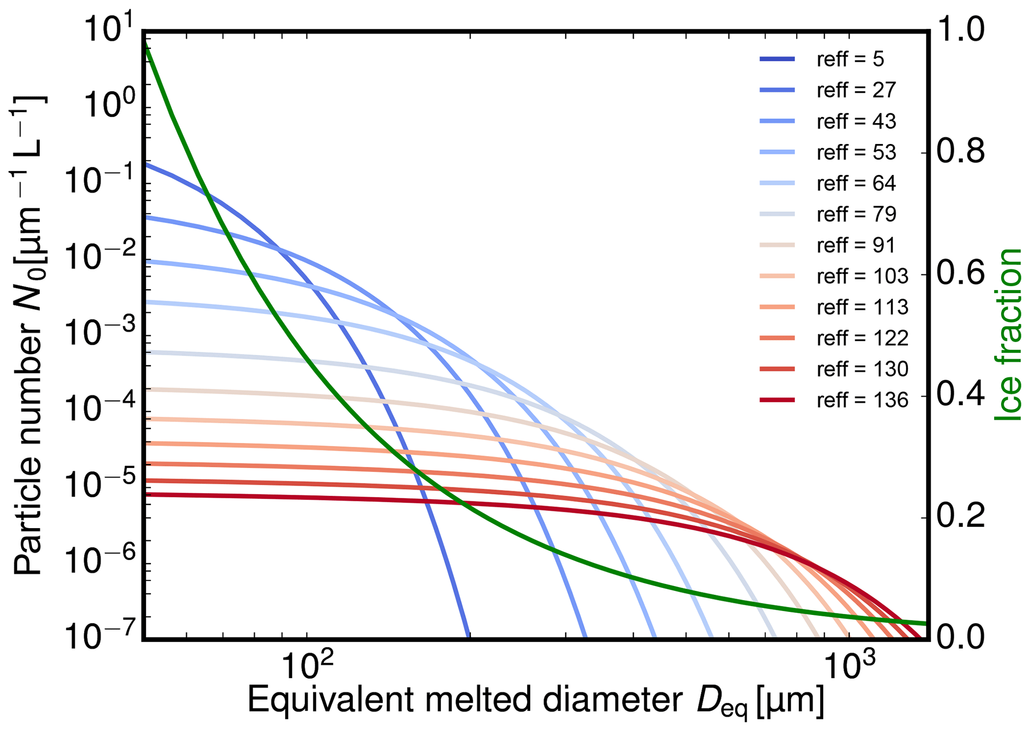
Figure 8The ice microphysical model used during the effective reflectivity study. The particle size distribution (Delanoë et al., 2005) and the mass–size relationship (green curve) (Heymsfield et al., 2010) are based on an extensive database of airborne in situ measurements.
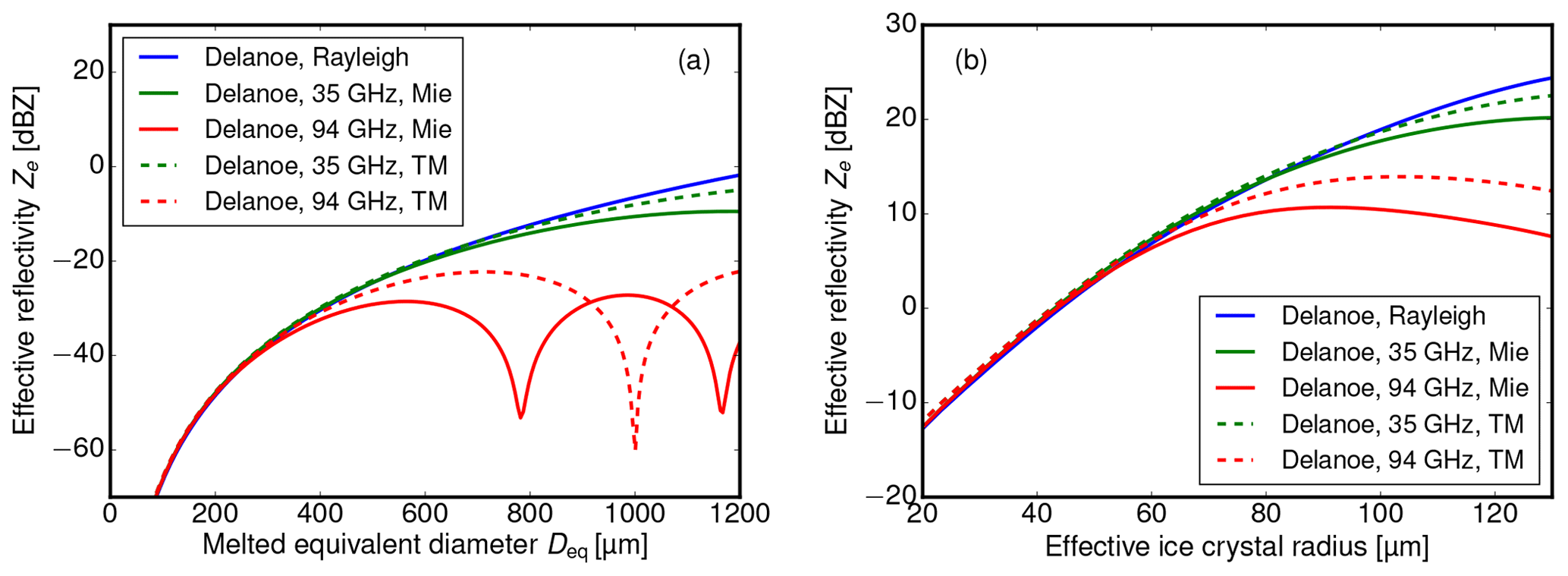
Figure 9Modeled effective reflectivities at 35 GHz (green) and 94 GHz (red) as a function of equivalent melted diameter Deq according to Rayleigh (blue), Mie (solid) and T-Matrix (dashed) theory. (a) Results for mono-disperse, horizontally aligned oblate spheroids with an aspect ratio of 0.6, composed of a mixture of air and ice according to Fig. 8. (b) Results for particle size distributions (shown in Fig. 8) of these spheroids with a fixed ice water content of 1 g m−1.
The model results for a single ice crystal are shown in Fig. 9a. Here, the effective reflectivities at 35 GHz (green) and 94 GHz (red) are shown as a function of equivalent melted diameter Deq according to Rayleigh (blue), Mie (solid) and T-Matrix (dashed) theory. While the effective reflectivity derived with Rayleigh theory increases with the square of the particle mass, Ze starts to deviate for Mie and T-Matrix theory for Deq>400 µm at 94 GHz and for Deq>800 µm at 35 GHz. For Deq larger than 600 µm (1200 µm), effective reflectivity for single ice spheroids decreases again for 94 GHz (resp. 35 GHz) due to Mie resonances. The reader is advised that the results in Fig. 9a probably underestimate the backscatter for snowflakes at larger Deq (Tyynelä et al., 2011).
In a next step, this result is integrated using the normalized PSDs for different effective radii. The results for a fixed ice water content of 1 g m−1 and variable effective ice crystal radius is shown in Fig. 9b.
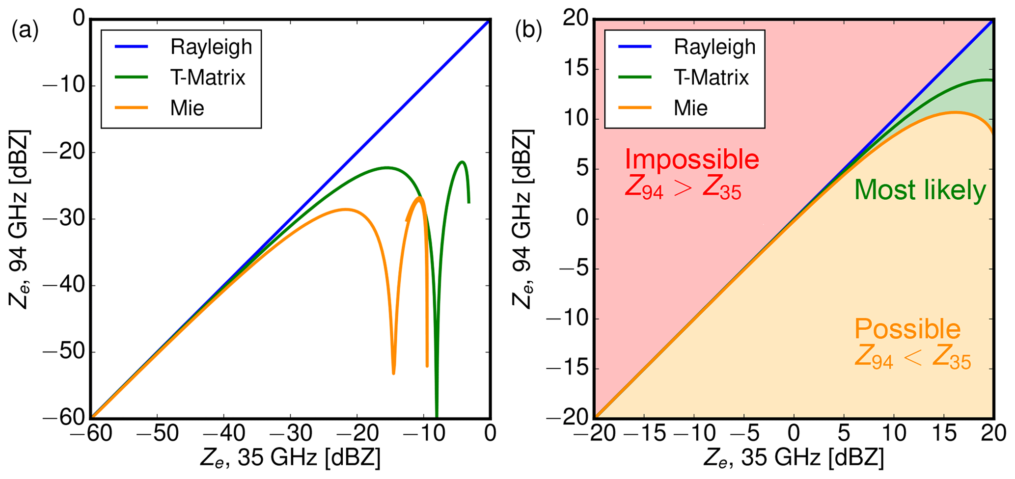
Figure 10Comparison between modeled effective reflectivities at 94 GHz against effective reflectivities at 35 GHz according to Rayleigh (blue), Mie (solid) and T-Matrix (dashed) theory. (a) Ze for mono-disperse ice crystals (soft spheroids), (b) Ze for the whole distribution shown in Fig. 8. Overall, the results for both wavelengths are almost identical for small particle sizes and thus small Ze, while Ze at 94 GHz is smaller than at 35 GHz for larger particles and thus larger Ze values.
Lower effective reflectivity values are almost identical, while larger effective reflectivities at 94 GHz are below the values at 35 GHz. For these realistic PSDs, effective reflectivities deviate from Rayleigh theory for effective radii larger than 80 µm at 94 GHz and 120 µm at 35 GHz. In Fig. 9b, the non-Rayleigh scattering effects become apparent at much smaller values of reff compared to values of Deq in Fig. 9a. This is only an apparent contradiction, since reff increases proportional to the ratio of mass to projected area and thereby much slower than Deq.
At last, the PSD-integrated results from Fig. 9b are used to constrain co-located Ze measurements at 35 and 94 GHz to physically plausible values. In Fig. 10, modeled effective reflectivities at 94 GHz are plotted against reflectivities at 35 GHz. The blue lines show the Rayleigh result, the solid lines show results according to Mie theory and the dashed lines show results for spheroids which where obtained from T-Matrix theory. Figure 10a shows results for mono-disperse ice particles with increasing Deq, while Fig. 10b shows results for whole ice crystal distributions with increasing reff and a fixed ice water content of 1 g m−1. Obviously, Ze values measured at 94 GHz should always be equal to or smaller than Ze values measured at 35 GHz. While Ze can also be much smaller due to the combination of non-Rayleigh scattering and higher attenuation at 94 GHz, ice clouds with smaller ice crystals and thus effective reflectivity should exhibit quite similar Ze values at 94 and 35 GHz.
5.2 RASTA
The calibration of the 94 GHz Doppler cloud radar named RASTA on board the French Falcon 20 was performed by Protat et al. (2009) with an absolute accuracy of 1 dB by using the ocean surface backscatter. In intercomparisons, they found that CloudSat measured about 1 dB higher reflectivities compared to RASTA. A coordinated flight with the French Falcon equipped with the 94 GHz radar system RASTA and the HALO equipped with the 35 GHz radar system was performed over southern France and northern Spain on 19 December 2013 between 11:00 and 11:15 UTC. Both aircraft flew in close separation of less than 5 min. During that leg, HALO was flying at an altitude of 13 km and passed the slower-flying French Falcon at an altitude of 10 km. The SEVIRI satellite image indicated a stratiform cloud in the measurement area (Fig. 11).
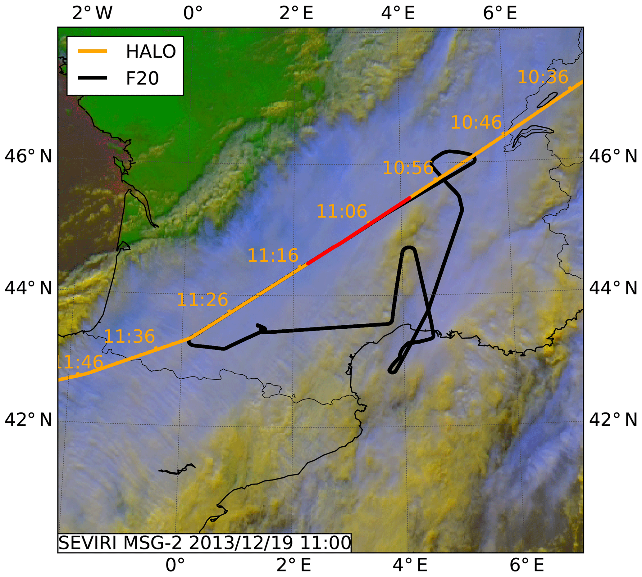
Figure 11SEVIRI satellite image for the coordinate flight leg between HALO and the French Falcon on 19 December 2013. The intercomparison between HAMP MIRA on HALO (orange line) and RASTA on the French Falcon (black line) was conducted over a deep ice cloud layer. The red line marks the coordinated flight leg over southern France between Lyon and Toulouse.
The radar measurements showed a two-layer cloud structure (Fig. 12) with a lower cloud in the first half of the measurement reaching from ground to about 4 km height and an overlying cloud layer, present during the whole co-located flight, with a cloud base between about 4.5 and 6 km height and an homogeneous cloud top at about 10.5 km in altitude. Thus, this coordinated flight provides an optimal measurement situation for a radar intercomparison.
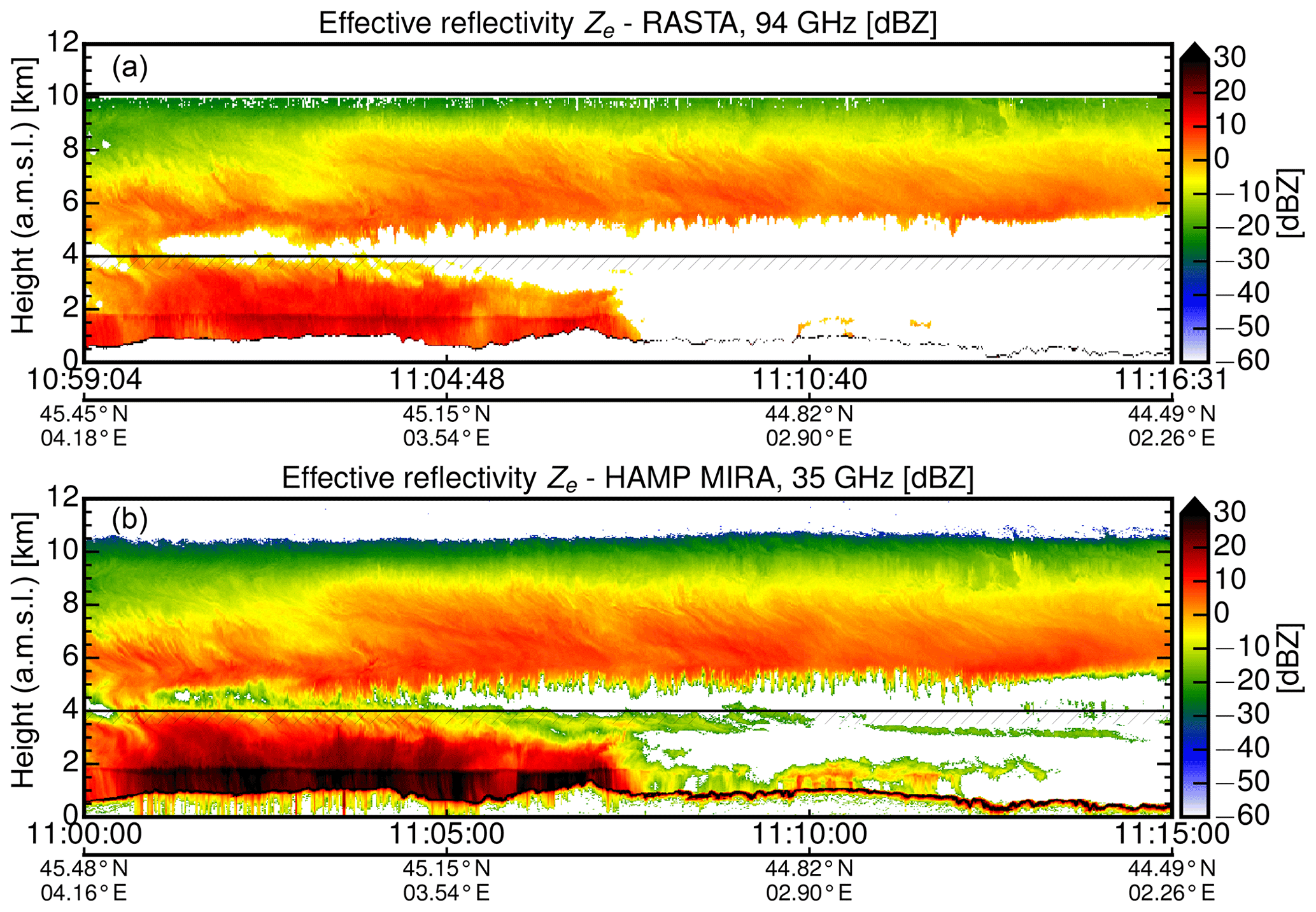
Figure 12Radar measurements performed with RASTA at 94 GHz (a) and HAMP MIRA at 35 GHz (b) along the coordinated flight track marked in Fig. 11. The reflectivity of HAMP MIRA was calculated using the new calibration. Cloud parts below 4 km (hatched line) were discarded in the direct comparison of Ze values in Fig. 13a to exclude effects caused by different attenuation or scattering regimes. The thin black line between 0.5 and 1.5 km shows the ground return of the Massif Central.
Due to the close separation of the aircraft, many cloud features can be found in both measurements at the same place. On the first sight of the measurements one can suggest that the HAMP MIRA instrument shows more variability within the cloud layer. Also, small-scale cloud structures are visible in the measurements made between 11:08 and 11:12 UTC. These cloud structures are not visible in the cross section of the RASTA measurements. At first glance, the HAMP MIRA at 35 GHz is more sensitive, especially to low-lying water clouds. While the effective reflectivities of the high cirrus cloud layer are quite similar, differences become visible in precipitating clouds, but also in non-precipitating water clouds after 11:07 UTC.
Like in Sect. 4.3, Ze was corrected for gaseous attenuation by oxygen and water vapor using the model of Rosenkranz (1998). Profiles of pressure, temperature and humidity were taken from the ECMWF Integrated Forecasting System (IFS) model. At first glance, Ze from both instruments looks quite similar in the cirrus cloud layer when using the new calibration of HAMP MIRA. In precipitating clouds at lower altitudes, however, differences in Ze become visible. As discussed in the previous model study, this can be explained by the difference in wavelength. With increasing ice crystal size, the transition from the Rayleigh scattering regime (Z≈D6) towards the Mie scattering regime (Z≈D2) first occurs at 94 GHz. The difference ΔZ between 94 and 35 GHz increases with increasing Ze due to larger ice crystals and higher attenuation at lower altitudes. In the following intercomparison, cloud parts below 4 km were thus discarded (hatched line in Fig. 12) to exclude effects caused by different attenuation or scattering regimes. Common coordinates were used as reference points to obtain reflectivity pairs from both instruments. Figure 13a gives a closer look: the airborne RASTA and MIRA HAMP measurements of Ze are compared against each other like in the model study shown in Fig. 10. On average, the linear regression reveals lower reflectivities (−1.4 dB) for RASTA. While slightly outside their calibration uncertainties, the agreement is still quite good with the slight time shift and wavelength difference in mind.
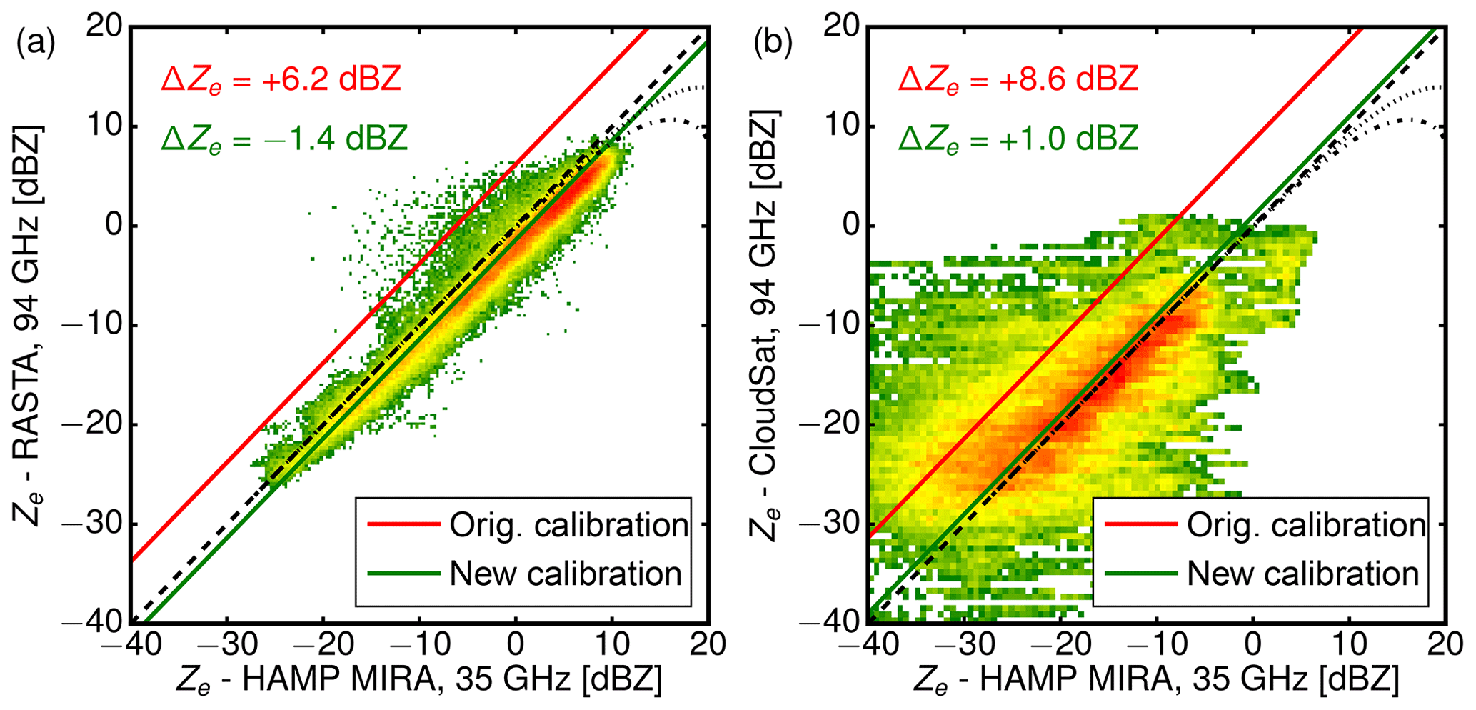
Figure 13(a) Comparison of effective reflectivities shown in Fig. 12 measured with HAMP MIRA at 35 GHz and the airborne RASTA instrument at 94 GHz. (b) Comparison of effective reflectivities shown in Fig. 14 measured with HAMP MIRA at 35 GHz and the spaceborne CloudSat instrument at 94 GHz. In both cases, common coordinates were used as reference points to obtain reflectivity pairs from both instruments. The green line shows the offset fit for the new calibration, the red line for the old HAMP MIRA calibration. The linear regression reveals lower reflectivities (−1.4 dB) for RASTA but slightly higher reflectivities (+1.0 dB) for CloudSat.
5.3 CloudSat
In recent years, CloudSat has been established as a reference source to compare the calibration of different ground- and airborne cloud radars (Protat et al., 2010). Due to the stability of its absolute calibration and its global coverage, CloudSat has tied the different cloud radar systems more closely together. For this reason, the spaceborne CloudSat is used in this last comparison. For intercomparison, a CloudSat underflight performed over the subtropical North Atlantic ocean east of Barbados on 17 August 2016 between 16:54 and 17:22 UTC (Fig. 14) is used. Due to the different conventions for the dielectric factor (|K|2=0.75 for Cloudsat, |K|2=0.93 for HAMP MIRA) the effective reflectivity from CloudSat first had to be converted for |K|2=0.93 using Eq. (1). Using a nearby dropsonde sounding, the two-way attenuation by water vapor and oxygen absorption was calculated at 35 and 94 GHz and used to correct Ze. For this underflight, Fig. 14a shows a corresponding image of the scene at a wavelength of 645 nm which was acquired by the wide-field camera (Pitts, 2007) on CALIPSO. HALO flew aligned with the CloudSat footprint for over 450 km. During this flight, all instrument settings were identical to the calibration flight (fp=6 kHz, τ=200 ns, 1 Hz), with footprints measuring approximately 100 m in the horizontal and 30 m in the vertical.

Figure 14CloudSat underflight performed with HALO over the subtropical North Atlantic Ocean east of Barbados on 17 August 2016. (a) Corresponding image along the common flight path which was acquired by the wide-field camera on CALIPSO. (b) Equivalent effective reflectivity Ze measured by the spaceborne CloudSat radar at 94 GHz and (c) by HAMP MIRA at 35 GHz. Again, cloud parts below 4 km (hatched line) were discarded in the direct comparison of Ze values in Fig. 13b.
In the beginning of the underpass flight, HALO was still climbing through the cirrus layer. Coinciding with the CloudSat overpass at 17:04 UTC, the aircraft then reached the top of the cirrus layer. The overall measurement scene is characterized by inhomogeneous cirrus cloud structures with a contribution of a few low clouds. The first part is dominated by an extended cirrus layer. As this cirrus layer becomes thinner, the second part is composed of broken and thinner cirrus clouds and shallow, convective marine boundary layer clouds. The cirrus layer and the lower precipitating clouds are clearly visible from both platforms. Strong effective reflectivity gradients are more blurred in the CloudSat measurement due to the coarser horizontal (1700 vs. 200 m) and vertical (500 vs. 30 m) resolution. For this reason, cloud edges as well as internal cloud structures are better resolved in the HAMP MIRA measurements. At cloud edges, this resolution-induced blurring leads to larger reflectivities while it reduces the maximum reflectivities found inside clouds. For the direct comparison in Fig. 13b, cloud parts below 4 km are again discarded (hatched line in Fig. 14) to exclude effects caused by different attenuation or scattering regimes. Again, common coordinates were used as reference points to obtain reflectivity pairs from both instruments. Since the scene is dominated by cirrus, the values for Ze are generally lower than in the RASTA-MIRA comparison. In contrast to the RASTA comparison, the linear regression reveals slightly larger reflectivities (+1.0 dB) for CloudSat. In comparison to Fig. 13a, the scatter between air- and spaceborne platforms is significantly larger due to the different spatial resolutions and instrument footprints. The small bias between CloudSat and HAMP MIRA is, however, within the calibration uncertainties of both instruments. The fact that the effective reflectivity measured by HAMP MIRA is in-between RASTA and CloudSat serves as further validation of the new absolute calibration.
In this study, we have characterized the absolute calibration of the microwave cloud radar HAMP MIRA, which is installed in the belly pod section of the German research aircraft HALO in a fixed nadir-pointing configuration. In the first step, the respective instrument components were characterized in the laboratory to obtain an internal calibration of the instrument. Our study confirmed the previously assumed antenna gain and the linearity of the receiver:
-
The antenna gain Ga=50.0 dBi and beam pattern (−3 dB beamwidth ϕ=0.56∘) showed no obvious asymmetries or increased side lobes.
-
With three attenuator settings (0, 15 and 30 dB), the radar receiver behaved very linearly (m=1.0009 and residual 0.054 dB) in a wide dynamic range of 70 dB from −105 to −5 dBm.
-
No further saturation by additional receiver components (e.g., mixers or filters) could be detected up to an input power of −5 dBm. This allows the dynamic range to be shifted by using the attenuator to measure higher input powers (which would otherwise be saturated) without losing the absolute calibration.
A key component of this work was the characterization of the spectral response of the radar receiver and its power transfer function 𝒯 using an analog continuous wave signal generator. This characterization gave valuable new insights into the receiver noise power and thus the receiver sensitivity. In the course of this study, the following major improvements to the instrument calibration were made:
-
The comparison of the measured and the previously estimated total receiver noise power (−95.3 vs. −98.2 dBm) revealed an underestimation of 2.9 dB.
-
This underestimation of Pn could be traced back to two different origins within the radar receiver
-
Spectral response measurements of the receiver unveiled a larger receiver noise bandwidth of 7.5 MHz, compared to the 5.0 MHz expected by the matched filter used (τr=200 ns). This issue could be traced back to an additional window function which was applied unintentionally to IQ data within the digital signal processor. The larger receiver response led to a somewhat higher thermal noise power PkTB (−106.9 vs. −105.2 dBm) than initially assumed.
-
The noise figure NF, describing the additional noise created by the receiver itself, turned out to be 1.1 dB larger than previously estimated, but showed no dependence on τr.
-
The combination of a larger spectral response (1.8 dB) and higher noise figure (1.1 dB) caused the 2.9 dB underestimation of the inherent noise power Pn. This, in turn, lead to an 2.9 dB underestimation of Ze.
-
Furthermore, no correction of the finite receiver bandwidth loss was applied to previous data sets of HAMP MIRA. Using the spectral response measurements, this study can now give an estimate for the finite receiver bandwidth loss Lfb of 1.2 dB.
In addition, our study re-evaluated the previously assumed attenuation by the belly pod and additional waveguides with the following measurements:
-
The thickness of the epoxy quartz radome in the belly pod was designed with a thickness of 4.53 mm to limit the one-way attenuation to around 0.5 dB. Deviations during manufacturing increased the planned belly pod thickness from 4.53 to 4.84 mm. This increased the one-way attenuation from the initially assumed value of 0.5 to 1.5 dB. The higher radome attenuation is now also confirmed by laboratory measurements.
-
The initially used calibration did not account for the losses caused by the longer waveguides in the airplane installation. With an additional length of 1.15 m and a specified attenuation of 0.65 dB m−1, the two-way attenuation by additional waveguides is 1.5 dB.
Subsequently, this component calibration was validated by using the ocean surface backscatter as a reference with known reflectivity. To this end, controlled roll maneuvers were flown during the NARVAL2 campaign in the vicinity of Barbados to sample the angular dependence of the ocean surface backscatter. The comparison with modeled backscatter values using the Cox–Munk model for non-slick ocean surfaces and measured values from the GPM satellite confirmed the internal calibration to within ±0.5 dB. In a second intercomparison study, the absolute accuracy of the internal calibration was further scrutinized during common flight legs with the airborne 94 GHz cloud radar RASTA and the spaceborne 94 GHz cloud radar CloudSat. To assess the influence of different radar wavelengths on this comparison, we first conducted a model study of effective reflectivities at 35 and 94 GHz. Using realistic ice particle size distributions, T-Matrix calculations for spheroids show almost identical effective reflectivities at 35 and 94 GHz for effective radii smaller than 50 µm. Larger ice crystals and higher attenuation generally lead to a smaller reflectivity at 94 GHz. In this context, the intercomparison showed good agreement between the HAMP MIRA at 35 and the RASTA at 94 GHz, with slightly lower reflectivities (−1.3 dB) for RASTA. The intercomparison with CloudSat showed slightly higher (+1.2 dB) reflectivities for CloudSat. These higher reflectivities were mostly found at cloud edges, where the coarser spatial resolution of CloudSat can blur out higher reflectivities into regions with thinner reflectivity below the sensitivity of CloudSat. The intercomparison studies showed that the absolute calibration uncertainty is now well below the initially required accuracy of 3 dB and even came close to the target accuracy of 1 dB.
In conclusion, the following procedures and techniques turned out to be essential for the absolute calibration of HAMP MIRA and should become state of the art:
-
The simultaneous characterization of the spectral response of the radar receiver and its power transfer function 𝒯 turned out to be very valuable to cross-check the receiver sensitivity Pn.
-
While Pn was previously estimated using an assumed receiver noise bandwidth B and a measured receiver noise factor Fn, it is now measured directly using a calibrated signal generator with adjustable power output.
-
Moreover, the signal generator should offer a frequency sweep mode to determine the spectral response to measure the receiver noise bandwidth B. A characterized spectral response is essential to calculate the finite receiver bandwidth loss Lfb. It can also be used to calculate the receiver sensitivity Pn.
-
The direct measurement of Pn and the calculated value can then be used to evaluate and check the receiver noise factor Fn. This should be done for two different matched filter lengths to characterize the dependence of Bn and Fn on τr.
-
Discrepancies between the component-wise calculation of Pn and the direct measurement can help to find additional noise sources or attenuation within the radar receiver.
-
Validate the budget approach of the internal calibration in intercomparison with external sources like sea surface data or different instruments.
The lessons learned in the course of this study helped us to better understand our instrument and increased the confidence in its absolute calibration. Subsequent studies for similar cloud radar instruments should consider following prerequisites and guidelines:
-
Knowledge about existing calibration offsets grows gradually. It is advisable to refrain from incremental updates of prior data sets. To mitigate confusion with different calibration offsets, a new calibration should only be applied to prior or current measurements when the internal calibration is in agreement with external reference sources.
-
Initially, the main focus should be on the antenna gain (including the radome) and the receiver sensitivity. The measured antenna gain and the radome attenuation should furthermore be cross-checked with calculated values.
-
For the characterization of the spectral response and receiver noise power, access to unprocessed Doppler spectra is advantageous to check the calculation of SNR independently.
-
The sole intercomparison of two cloud radars is a necessary but not sufficient step towards an absolute calibration. An apparent agreement can lead to a false sense of accuracy since common misconceptions and assumptions remain hidden and can thus propagate from instrument to instrument. Discrepancies in intercomparisons should always trigger a re-evaluation of the internal calibration.
-
While a sole internal calibration can help to get a better understanding of the instrument performance, it has to be validated with external reference sources. It is the combination of internal calibration and external validation which establishes trust in the absolute calibration.
The recalibrated data set of HAMP MIRA is available in Earth System Science Data with the identifier https://doi.org/10.1594/WDCC/HALO_measurements_1, https://doi.org/10.1594/WDCC/HALO_measurements_2, https://doi.org/10.1594/WDCC/HALO_measurements_3, https://doi.org/10.1594/WDCC/HALO_measurements_4. The data set is described in detail in Konow et al. (2019), https://doi.org/10.5194/essd-2018-116. All data sets created during the internal calibration are provided upon request.
In-flight thermistor measurements of the average transmit power 〈Pt〉 proved to be unreliable due to strong variations in ambient temperatures in the cabin. For this reason, thermally controlled measurements of 〈Pt〉 were conducted at ground level which were correlated with measured magnetron currents Im. The relationship between both parameters then allowed 〈Pt〉 to be derived from in-flight measurements of Im. For this analysis, we operated the HAMP MIRA instrument within a trailer during a 27-day ground-based test campaign in 2016. We observed the magnetron temperature Tmg and the magnetron anode current Img for two different anode voltages (15.4 and 15.5 kV). The average transmit power 〈Pt〉 was measured every 30 min using a calibrated thermistor. Fig. A1a shows the relationship between magnetron temperature Tmg and magnetron anode current Img. The relationship between magnetron anode current Img and average transmit power 〈Pt〉 is given in Fig. A1b. Depending on the anode voltage, 〈Pt〉 increased linearly with Img and varied by 0.2 dB within the operational range of Tmg between 25 and 35 ∘C.
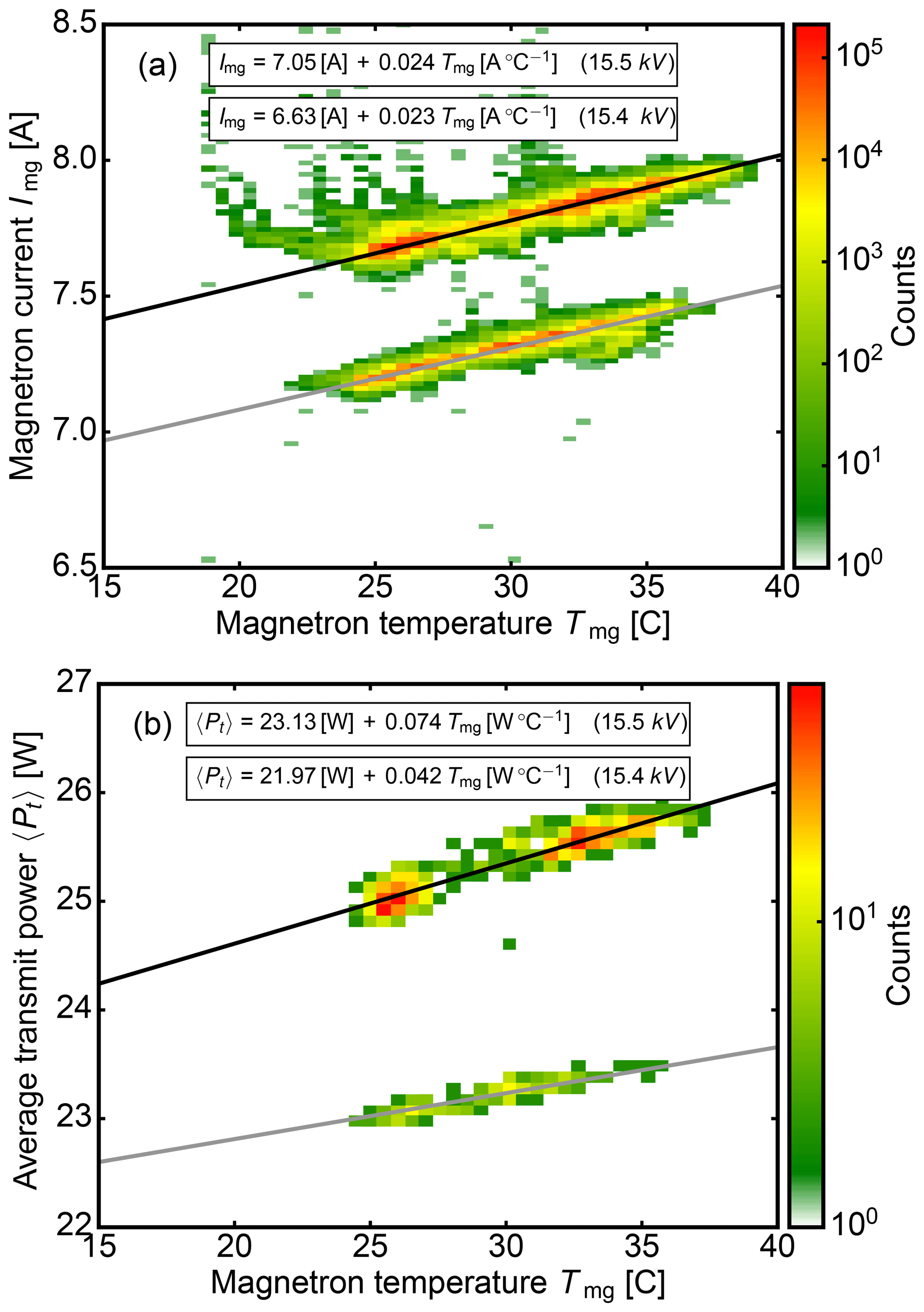
Figure A1Analysis of the relationship between magnetron temperature Tmg, magnetron anode current Img and average transmit power 〈Pt〉 during a 27-day ground-based test campaign in 2016 for two different anode voltages (15.4 and 15.5 kV). (a) Relationship between magnetron temperature Tmg and magnetron anode current Img. (b) Relationship between magnetron anode current Img and average transmit power 〈Pt〉.
The thickness of the epoxy quartz radome in the belly pod was designed with a thickness d of 4.53 mm to limit the one-way attenuation to around 0.5 dB. The thickness was designed to cancel out reflections on the front and back side of the radome. However, laboratory measurements of the finished radome found a one-way attenuation of around 1.5 dB for the transmit frequency 35.5 GHz of HAMP MIRA. The spectral transmission of the radome between 26 and 40 GHz is shown in Fig. B1a. The red line shows the initially assumed spectral transmission using a relative permittivity ϵr=3.44, a dielectric loss tangent tan δ=0.0015 and a radome thickness d=4.53 mm. Our measurements (black crosses), however, can be better explained by the green line in Fig. B1a, which shows the spectral transmission for a relative permittivity ϵr=3.80, a dielectric loss tangent tan δ=0.0017 and a radome thickness d=4.84 mm. In Fig. B1b, the transmission for both material properties are compared as a function of the radome thickness d. The oscillating transmission can be explained by the cancellation of reflections at every half-wavelength. Since the wavelength is shorter within the radome material (ϵr=3.80), this happens every mm at 35.5 GHz. The combination of a higher relative permittivity and the slight increase in radome thickness can explain the 1 dB increase in radome attenuation.
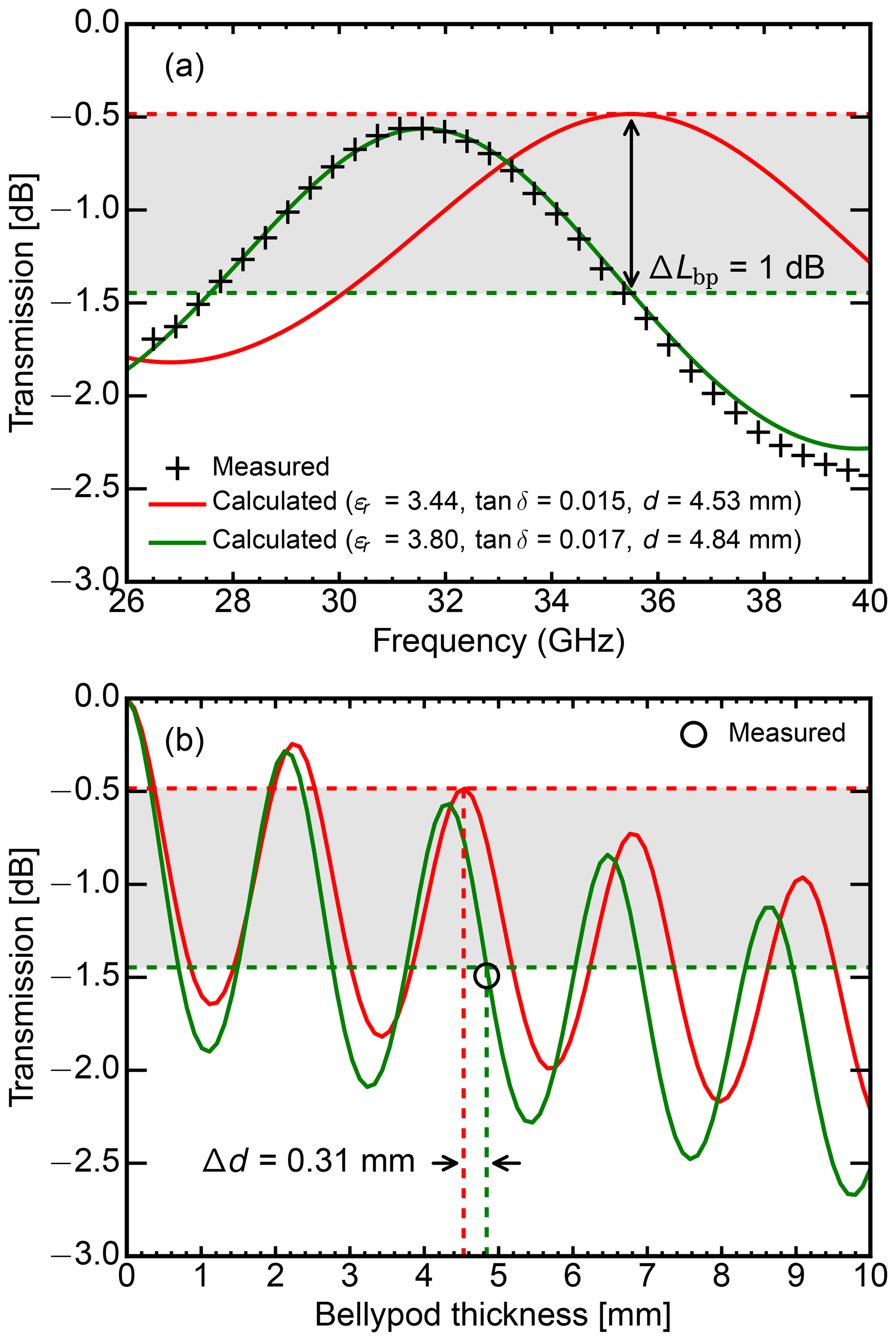
Figure B1Analysis of the belly pod radome transmission of HALO. (a) Radome transmission between 26 and 40 GHz for the initially assumed material properties (red line, ϵr=3.44, tan δ=0.0015, d=4.53 mm) and the measured ones (red line, ϵr=3.80, tan δ=0.0017, d=4.84 mm). (b) Radome transmission for the two material properties (red: assumed, green: measured) as a function of the radome thickness d. A increase in relative permittivity and thickness (Δ=0.31 mm) increased the radome attenuation by 1 dB.
FE and MBP conceived the concept for the internal calibration. FE, MBP, MH and LH performed the internal calibration and the airborne measurements. FE developed the presented methods and carried out the analysis. FE, MBP and MH contributed to the interpretation of the results. JD provided the single scattering results and RASTA measurements. FE took the lead in writing the paper. All authors provided feedback on the paper.
The authors declare that they have no conflict of interest.
This work was jointly supported by the German Aerospace Center (DLR), the Max
Planck Society (MPI) and the German Research Foundation (DFG) through the
HALO Priority Program SPP 1294, “Atmospheric and Earth System Research
with the Research Aircraft HALO (High Altitude and Long Range Research Aircraft)”. Measurement equipment was kindly provided by DLR-HR. DLR-FX and
its pilots are thanked for their great support during research flights. GPM
data were provided by the NASA/Goddard Space Flight Center's PPS team, which
develop and compute the “GPM DPR Ka vertical profile precipitation
swath retrievals” (https://doi.org/10.5067/GPM/DPR/Ka/2A/04) as a contribution to GPM.
The authors thank Oliver Lux for his internal review of the
paper.
The article processing charges for this open-access
publication were covered by a Research
Centre of the Helmholtz Association.
Edited by: Vassilis Amiridis
Reviewed by: three anonymous referees
Acquistapace, C., Kneifel, S., Löhnert, U., Kollias, P., Maahn, M., and Bauer-Pfundstein, M.: Optimizing observations of drizzle onset with millimeter-wavelength radars, Atmos. Meas. Tech., 10, 1783–1802, https://doi.org/10.5194/amt-10-1783-2017, 2017. a
Agilent Technologies: Noise Figure Measurement Accuracy – The Y-Factor Method, Application Note 57-2, available at: http://literature.cdn.keysight.com/litweb/pdf/5952-3706E.pdf (last access: 10 March 2019), October 2004. a
Apel, J. R.: An improved model of the ocean surface wave vector spectrum and its effects on radar backscatter, J. Geophys. Res.-Oceans, 99, 16269–16291, https://doi.org/10.1029/94JC00846, 1994. a
Atlas, D.: Radar Calibration: Some Simple Approaches, B. Am. Meteorol. Soc., 83, 1313–1316, https://doi.org/10.1175/1520-0477(2002)083<1313:RCSSA>2.3.CO;2, 2002. a
Barrick, D. E., Headrick, J. M., Bogle, R. W., and Crombie, D. D.: Sea backscatter at HF: Interpretation and utilization of the echo, Proc. IEEE, 62, 673–680, https://doi.org/10.1109/PROC.1974.9507, 1974. a
Bauer-Pfundstein, M. and Görsdorf, U.: Target separation and classification using cloud radar Doppler-spectra, in: Proceedings 33rd Intern. Conf. on Radar Meteorology, Cairns, available at: http://ams.confex.com/ams/33Radar/techprogram/paper_123456.htm (last access: 10 March 2019), 2007. a
Bormotov, V., Peters, G., Schünemann, K., Vavriv, D., Vinogradov, V., and Volkov, V.: 36 GHz Doppler radar for remote sensing of the atmosphere, in: Proceedings of Millennium Conference on Antenna and Propagation, Davos Switzerland, pp. 9–14, 2000. a
Boucher, O., Randall, D., Artaxo, P., Bretherton, C., Feingold, G., Forster, P., Kerminen, V.-M., Kondo, Y., Liao, H., Lohmann, U., Rasch, P., Satheesh, S., Sherwood, S., Stevens, B., and Zhang, X.: Clouds and Aerosols, book section 7, pp. 571–658, Cambridge University Press, Cambridge, United Kingdom and New York, NY, USA, https://doi.org/10.1017/CBO9781107415324.016, 2013. a
Bouniol, D., Protat, A., Plana-Fattori, A., Giraud, M., Vinson, J.-P., and Grand, N.: Comparison of Airborne and Spaceborne 95-GHz Radar Reflectivities and Evaluation of Multiple Scattering Effects in Spaceborne Measurements, J. Atmos. Ocean. Tech., 25, 1983–1995, https://doi.org/10.1175/2008JTECHA1011.1, 2008. a, b
Brown, G. S.: Quasi-Specular Scattering from the Air-Sea Interface, in: Surface Waves and Fluxes, Environmental Fluid Mechanics, pp. 1–39, Springer, Dordrecht, https://doi.org/10.1007/978-94-009-0627-3_1, 1990. a
Caylor, I. J..: NASA ER-2 Doppler radar reflectivity calibration for the CAMEX project, Tech. rep., Goddard Space Flight Center. Greenbelt, Maryland, available at: https://ntrs.nasa.gov/search.jsp?R=19940033279 (last access: 10 March 2019), 1994. a
Caylor, I. J., Heymsfield, G. M., Meneghini, R., and Miller, L. S.: Correction of Sampling Errors in Ocean Surface Cross-Sectional Estimates from Nadir-Looking Weather Radar, J. Atmos. Ocean. Tech., 14, 203–210, https://doi.org/10.1175/1520-0426(1997)014<0203:COSEIO>2.0.CO;2, 1997. a, b
Chandrasekar, V., Baldini, L., Bharadwaj, N., and Smith, P. L.: Calibration procedures for global precipitation-measurement ground-validation radars, URSI Radio Science Bulletin, 355, 45–73, 2015. a
Chen, T., Zhang, Y., and Rossow, W.: Sensitivity of atmospheric radiative heating rate profiles to variations of cloud layer overlap, J. Climate, 13, 2941–2959, 2000. a
Cox, C. and Munk, W.: Measurement of the roughness of the sea surface from photographs of the sun's glitter, J. Opt. Soc. Am., 44, 838–850, 1954. a
Delanoë, J. and Hogan, R. J.: A variational scheme for retrieving ice cloud properties from combined radar, lidar, and infrared radiometer, J. Geophys. Res., 113, D07204, https://doi.org/10.1029/2007JD009000, 2008. a, b
Delanoë, J., Protat, A., Testud, J., Bouniol, D., Heymsfield, A. J., Bansemer, A., Brown, P. R. A., and Forbes, R. M.: Statistical properties of the normalized ice particle size distribution, J. Geophys. Res.-Atmos., 110, D10201, https://doi.org/10.1029/2004JD005405, 2005. a, b
Delanoë, J. M. E., Heymsfield, A. J., Protat, A., Bansemer, A., and Hogan, R. J.: Normalized particle size distribution for remote sensing application, J. Geophys. Res.-Atmos., 119, 4204–4227, https://doi.org/10.1002/2013JD020700, 2014. a, b
Deng, M., Mace, G. G., Wang, Z., and Okamoto, H.: Tropical Composition, Cloud and Climate Coupling Experiment validation for cirrus cloud profiling retrieval using CloudSat radar and CALIPSO lidar, J. Geophys. Res.-Atmos., 115, D00J15, https://doi.org/10.1029/2009JD013104, 2010. a
Donovan, D. P., van Lammeren, A., Hogan, R., Russchenberg, H., Apituley, A., Francis, P., Testud, J., Pelon, J., Quante, M., and Agnew, J.: Combined radar and lidar cloud remote sensing: Comparison with IR radiometer and in-situ measurements, Phys. Chem. Earth B, 25, 1049–1055, 2000. a
Doviak, R. J. and Zrnić, D.: Receiver Bandwidth Effect on Reflectivity and Doppler Velocity Estimates, J. Appl. Meteorol., 18, 69–76, https://doi.org/10.1175/1520-0450(1979)018<0069:RBEORA>2.0.CO;2, 1979. a
Doviak, R. J. and Zrnić, D. S.: Doppler Radar and Weather Observations, Dover Publications, Mineola, New York, 2006. a, b
Durden, S. L., Im, E., Li, F. K., Ricketts, W., Tanner, A., and Wilson, W.: ARMAR: An Airborne Rain-Mapping Radar, J. Atmos. Ocean. Tech., 11, 727–737, https://doi.org/10.1175/1520-0426(1994)011<0727:AAARMR>2.0.CO;2, 1994. a
Ewald, F., Winkler, C., and Zinner, T.: Reconstruction of cloud geometry using a scanning cloud radar, Atmos. Meas. Tech., 8, 2491–2508, https://doi.org/10.5194/amt-8-2491-2015, 2015. a
Foot, J. S.: Some observations of the optical properties of clouds. II: Cirrus, Q. J. Roy. Meteorol. Soc., 114, 145–164, 1988. a
Freilich, M. H. and Vanhoff, B. A.: The Relationship between Winds, Surface Roughness, and Radar Backscatter at Low Incidence Angles from TRMM Precipitation Radar Measurements, J. Atmos. Ocean. Tech., 20, 549–562, https://doi.org/10.1175/1520-0426(2003)20<549:TRBWSR>2.0.CO;2, 2003. a, b
Görsdorf, U., Lehmann, V., Bauer-Pfundstein, M., Peters, G., Vavriv, D., Vinogradov, V., and Volkov, V.: A 35-GHz Polarimetric Doppler Radar for Long-Term Observations of Cloud Parameters – Description of System and Data Processing, J. Atmos. Ocean. Tech., 32, 675–690, https://doi.org/10.1175/JTECH-D-14-00066.1, 2015. a, b
Haimov, S. and Rodi, A.: Fixed-Antenna Pointing-Angle Calibration of Airborne Doppler Cloud Radar, J. Atmos. Ocean. Tech., 30, 2320–2335, https://doi.org/10.1175/JTECH-D-12-00262.1, 2013. a
Handwerker, J. and Miller, M. A.: Intercomparison of measurements obtained by vertically pointing collocated 95 GHz and 35.5 GHz cloud radars, in: Proc. Fifth European Conference on Radar in Meteorology and Hydrology, 2008. a
Hennemuth, B., Weiss, A., Bösenberg, J., Jacob, D., Linné, H., Peters, G., and Pfeifer, S.: Quality assessment of water cycle parameters in REMO by radar-lidar synergy, Atmos. Chem. Phys., 8, 287–308, https://doi.org/10.5194/acp-8-287-2008, 2008. a
Heymsfield, A. J., Schmitt, C., Bansemer, A., and Twohy, C. H.: Improved Representation of Ice Particle Masses Based on Observations in Natural Clouds, J. Atmos. Sci., 67, 3303–3318, 2010. a, b, c
Heymsfield, G. M., Bidwell, S. W., Caylor, I. J., Ameen, S., Nicholson, S., Boncyk, W., Miller, L., Vandemark, D., Racette, P. E., and Dod, L. R.: The EDOP Radar System on the High-Altitude NASA ER-2 Aircraft, J. Atmos. Ocean. Tech., 13, 795–809, https://doi.org/10.1175/1520-0426(1996)013<0795:TERSOT>2.0.CO;2, 1996. a
Horie, H. and Takahashi, N.: External calibration method using sea surface scattering for satelliteborne W-band cloud profiling radar, Proc. ISPRS, 38, 160–163, 2010. a
Horie, H., Iguchi, T., Hanado, H., Kuroiwa, H., Okamoto, H., and Kumagai, H.: Development of a 95-GHz Airborne Cloud Profiling Radar (SPIDER) – Technical Aspects, IEICE TRANSACTIONS on Communications, E83-B, 2010–2020, 2000. a
Horie, H., Kuroiwa, H., and Kumagai, H.: Near nadir scattering properties at W-band frequency for the sea surface, in: IGARSS 2004. 2004 IEEE International Geoscience and Remote Sensing Symposium, 3, 1742–1745, https://doi.org/10.1109/IGARSS.2004.1370669, 2004. a, b
Hou, A. Y., Kakar, R. K., Neeck, S., Azarbarzin, A. A., Kummerow, C. D., Kojima, M., Oki, R., Nakamura, K., and Iguchi, T.: The Global Precipitation Measurement Mission, B. Am. Meteorol. Soc., 95, 701–722, https://doi.org/10.1175/BAMS-D-13-00164.1, 2013. a
Illingworth, A. J., Hogan, R. J., O'Connor, E. J., Bouniol, D., Delanoë, J., Pelon, J., Protat, A., Brooks, M. E., Gaussiat, N., Wilson, D. R., Donovan, D. P., Baltink, H. K., van Zadelhoff, G.-J., Eastment, J. D., Goddard, J. W. F., Wrench, C. L., Haeffelin, M., Krasnov, O. A., Russchenberg, H. W. J., Piriou, J.-M., Vinit, F., Seifert, A., Tompkins, A. M., and Willén, U.: Cloudnet Continuous Evaluation of Cloud Profiles in Seven Operational Models Using Ground-Based Observations, B. Am. Meteorol. Soc., 88, 883–898, https://doi.org/10.1175/BAMS-88-6-883, 2007. a
Illingworth, A. J., Barker, H. W., Beljaars, A., Ceccaldi, M., Chepfer, H., Clerbaux, N., Cole, J., Delanoë, J., Domenech, C., Donovan, D. P., Fukuda, S., Hirakata, M., Hogan, R. J., Huenerbein, A., Kollias, P., Kubota, T., Nakajima, T., Nakajima, T. Y., Nishizawa, T., Ohno, Y., Okamoto, H., Oki, R., Sato, K., Satoh, M., Shephard, M. W., Velázquez-Blázquez, A., Wandinger, U., Wehr, T., and van Zadelhoff, G.-J.: The EarthCARE Satellite: The Next Step Forward in Global Measurements of Clouds, Aerosols, Precipitation, and Radiation, B. Am. Meteorol. Soc., 96, 1311–1332, https://doi.org/10.1175/BAMS-D-12-00227.1, 2014. a, b
Intrieri, J. M., Stephens, G. L., Eberhard, W. L., and Uttal, T.: A Method for Determining Cirrus Cloud Particle Sizes Using Lidar and Radar Backscatter Technique, J. Appl. Meteorol., 32, 1074–1082, https://doi.org/10.1175/1520-0450(1993)032<1074:AMFDCC>2.0.CO;2, 1993. a
Jackson, F. C., Walton, W. T., Hines, D. E., Walter, B. A., and Peng, C. Y.: Sea surface mean square slope from Ku-band backscatter data, J. Geophys. Res., 97, 11411–11427, https://doi.org/10.1029/92JC00766, 1992. a, b
Klein, L. and Swift, C.: An improved model for the dielectric constant of sea water at microwave frequencies, IEEE J. Oceanic Eng., 2, 104–111, https://doi.org/10.1109/JOE.1977.1145319, 1977. a
Konow, H., Jacob, M., Ament, F., Crewell, S., Ewald, F., Hagen, M., Hirsch, L., Jansen, F., Mech, M., and Stevens, B.: A unified data set of airborne cloud remote sensing using the HALO Microwave Package (HAMP), Earth Syst. Sci. Data Discuss., https://doi.org/10.5194/essd-2018-116, in review, 2019. a
Krautstrunk, M. and Giez, A.: The Transition From FALCON to HALO Era Airborne Atmospheric Research, in: Atmospheric Physics, edited by: Schumann, U., Research Topics in Aerospace, pp. 609–624, Springer Berlin Heidelberg, available at: http://link.springer.com/chapter/10.1007/978-3-642-30183-4_37 (last access: 10 March 2019), 2012. a
Li, L., Heymsfield, G. M., Racette, P. E., Tian, L., and Zenker, E.: A 94-GHz Cloud Radar System on a NASA High-Altitude ER-2 Aircraft, J. Atmos. Ocean. Tech., 21, 1378–1388, https://doi.org/10.1175/1520-0426(2004)021<1378:AGCRSO>2.0.CO;2, 2004. a
Li, L., Heymsfield, G. M., Tian, L., and Racette, P. E.: Measurements of Ocean Surface Backscattering Using an Airborne 94-GHz Cloud Radar – Implication for Calibration of Airborne and Spaceborne W-Band Radars, J. Atmos. Ocean. Tech., 22, 1033–1045, https://doi.org/10.1175/JTECH1722.1, 2005. a, b, c, d
Li, Z., Cribb, M., Chang, F.-L., Trishchenko, A., and Luo, Y.: Natural variability and sampling errors in solar radiation measurements for model validation over the Atmospheric Radiation Measurement Southern Great Plains region, J. Geophys. Res., 110, D15S19, https://doi.org/10.1029/2004JD005028, 2005. a, b, c, d
Lonitz, K., Stevens, B., Nuijens, L., Sant, V., Hirsch, L., and Seifert, A.: The Signature of Aerosols and Meteorology in Long-Term Cloud Radar Observations of Trade Wind Cumuli, J. Atmos. Sci., 72, 4643–4659, https://doi.org/10.1175/JAS-D-14-0348.1, 2015. a
Maahn, M. and Kollias, P.: Improved Micro Rain Radar snow measurements using Doppler spectra post-processing, Atmos. Meas. Tech., 5, 2661–2673, https://doi.org/10.5194/amt-5-2661-2012, 2012. a
Masuko, H., Okamoto, K., Shimada, M., and Niwa, S.: Measurement of microwave backscattering signatures of the ocean surface using X band and Ka band airborne scatterometers, J. Geophys. Res.-Oceans, 91, 13065–13083, https://doi.org/10.1029/JC091iC11p13065, 1986. a
Mech, M., Orlandi, E., Crewell, S., Ament, F., Hirsch, L., Hagen, M., Peters, G., and Stevens, B.: HAMP – the microwave package on the High Altitude and LOng range research aircraft (HALO), Atmos. Meas. Tech., 7, 4539–4553, https://doi.org/10.5194/amt-7-4539-2014, 2014. a, b, c, d
Meissner, T. and Wentz, F. J.: The complex dielectric constant of pure and sea water from microwave satellite observations, IEEE T. Geosci. Remote, 42, 1836–1849, https://doi.org/10.1109/TGRS.2004.831888, 2004. a
Myagkov, A., Seifert, P., Wandinger, U., Bauer-Pfundstein, M., and Matrosov, S. Y.: Effects of Antenna Patterns on Cloud Radar Polarimetric Measurements, J. Atmos. Ocean. Tech., 32, 1813–1828, 2015. a
Myagkov, A., Seifert, P., Wandinger, U., Bühl, J., and Engelmann, R.: Relationship between temperature and apparent shape of pristine ice crystals derived from polarimetric cloud radar observations during the ACCEPT campaign, Atmos. Meas. Tech., 9, 3739–3754, https://doi.org/10.5194/amt-9-3739-2016, 2016. a
Nouguier, F., Mouche, A., Rascle, N., Chapron, B., and Vandemark, D.: Analysis of Dual-Frequency Ocean Backscatter Measurements at Ku- and Ka-Bands Using Near-Nadir Incidence GPM Radar Data, IEEE Geosci. Remote S., 13, 1310–1314, https://doi.org/10.1109/LGRS.2016.2583198, 2016. a
Pitts, M. C., Thomason, L. W., Hu, Y., and Winker, D. M.: An assessment of the on-orbit performance of the CALIPSO wide field camera, Proc. SPIE 6745, Remote Sensing of Clouds and the Atmosphere XII, 67450K, 2007. a
Plant, W. J.: A stochastic, multiscale model of microwave backscatter from the ocean, J. Geophys. Res.-Oceans, 107, 3120, https://doi.org/10.1029/2001JC000909, 2002. a
Protat, A., Pelon, J., Grand, N., Delville, P., Laborie, P., Vinson, J.-P., Bouniol, D., Bruneau, D., Chepfer, H., Delanoë, J., Haeffelin, M., Noel, V., and Tinel, C.: The Rali project: combining a radar and a lidar for the study of weakly-precipitating clouds, available at: http://hdl.handle.net/2042/36076 (last access: 10 March 2019), 2004. a
Protat, A., Bouniol, D., Delanoë, J., O'Connor, E., May, P. T., Plana-Fattori, A., Hasson, A., Görsdorf, U., and Heymsfield, A. J.: Assessment of Cloudsat Reflectivity Measurements and Ice Cloud Properties Using Ground-Based and Airborne Cloud Radar Observations, J. Atmos. Ocean. Tech., 26, 1717–1741, https://doi.org/10.1175/2009JTECHA1246.1, 2009. a, b, c, d
Protat, A., Bouniol, D., O'Connor, E. J., Klein Baltink, H., Verlinde, J., and Widener, K.: CloudSat as a Global Radar Calibrator, J. Atmos. Ocean. Tech., 28, 445–452, https://doi.org/10.1175/2010JTECHA1443.1, 2010. a, b
Protat, A., Delanoë, J., Strapp, J. W., Fontaine, E., Leroy, D., Schwarzenboeck, A., Lilie, L., Davison, C., Dezitter, F., Grandin, A., and Weber, M.: The Measured Relationship between Ice Water Content and Cloud Radar Reflectivity in Tropical Convective Clouds, J. Appl. Meteorol. Climatol., 55, 1707–1729, https://doi.org/10.1175/JAMC-D-15-0248.1, 2016. a
Ray, P. S.: Broadband complex refractive indices of ice and water, Appl. Optics, 11, 1836, https://doi.org/10.1364/AO.11.001836, 1972. a
Riddle, A. C., Hartten, L. M., Carter, D. A., Johnston, P. E., and Williams, C. R.: A Minimum Threshold for Wind Profiler Signal-to-Noise Ratios, J. Atmos. Ocean. Tech., 29, 889–895, 2012. a
Rosenkranz, P. W.: Water vapor microwave continuum absorption: A comparison of measurements and models, Radio Sci., 33, 919–928, https://doi.org/10.1029/98RS01182, 1998. a, b
Sadowy, G. A., Berkun, A. C., Chun, W., Im, E., and Durden, S. L.: Development of an advanced airborne precipitation radar, Microwave J., 46, 84–86, 2003. a
Stephens, G., Vane, D., Boain, R., Mace, G., Sassen, K., Wang, Z., Illingworth, A., O'Connor, E., Rossow, W., Durden, S., Miller, S., Austin, R., Benedetti, A., Mitrescu, C., and the CloudSat Science Team: The CloudSat mission and the A-train, B. Am. Meteorol. Soc., 83, 1771–1790, 2002. a, b, c
Stubenrauch, C. J., Rossow, W. B., Kinne, S., Ackerman, S., Cesana, G., Chepfer, H., Di Girolamo, L., Getzewich, B., Guignard, A., Heidinger, A., Maddux, B. C., Menzel, W. P., Minnis, P., Pearl, C., Platnick, S., Poulsen, C., Riedi, J., Sun-Mack, S., Walther, A., Winker, D., Zeng, S., and Zhao, G.: Assessment of Global Cloud Datasets from Satellites: Project and Database Initiated by the GEWEX Radiation Panel, B. Am. Meteorol. Soc., 94, 1031–1049, https://doi.org/10.1175/BAMS-D-12-00117.1, 2013. a
Tanelli, S., Durden, S. L., and Im, E.: Simultaneous Measurements of Ku- and Ka-Band Sea Surface Cross Sections by an Airborne Radar, IEEE Geosci. Remote S., 3, 359–363, https://doi.org/10.1109/LGRS.2006.872929, 2006. a, b, c, d
Tanelli, S., Durden, S. L., Im, E., Pak, K. S., Reinke, D. G., Partain, P., Haynes, J. M., and Marchand, R. T.: CloudSat's Cloud Profiling Radar After Two Years in Orbit: Performance, Calibration, and Processing, IEEE T. Geosci. Remote, 46, 3560–3573, https://doi.org/10.1109/TGRS.2008.2002030, 2008. a, b
Tyynelä, J., Leinonen, J., Moisseev, D., and Nousiainen, T.: Radar Backscattering from Snowflakes: Comparison of Fractal, Aggregate, and Soft Spheroid Models, J. Atmos. Ocean. Tech., 28, 1365–1372, 2011. a
Valenzuela, G. R.: Theories for the interaction of electromagnetic and oceanic waves – A review, Bound.-Lay. Meteorol., 13, 61–85, https://doi.org/10.1007/BF00913863, 1978. a, b, c
Vavriv, D. M., Volkov, V. A., Bormotov, V. N., Vynogradov, V. V., Kozhyn, R. V., Trush, B. V., Belikov, A. A., and Semenyuta, V. Y.: Millimeter-wave radars for environmental studies, Telecomm. Radio Eng.+, 61, 292–313, https://doi.org/10.1615/TelecomRadEng.v61.i4.30, 2004. a
Vega, M. A., Chandrasekar, V., Nguyen, C., Mishra, K. V., and Carswell, J.: Calibration of the NASA Dual-Frequency, Dual-Polarized, Doppler Radar, 2012 IEEE International Geoscience and Remote Sensing Symposium, Munich, 4625–4628, https://doi.org/10.1109/IGARSS.2012.6350435, 2012. a
Wu, J.: Mean square slopes of the wind-disturbed water surface, their magnitude, directionality, and composition, Radio Sci., 25, 37–48, https://doi.org/10.1029/RS025i001p00037, 1990. a
Zhao, C., Xie, S., Klein, S. A., Protat, A., Shupe, M. D., McFarlane, S. A., Comstock, J. M., Delanoë, J., Deng, M., Dunn, M., Hogan, R. J., Huang, D., Jensen, M. P., Mace, G. G., McCoy, R., O'Connor, E. J., Turner, D. D., and Wang, Z.: Toward understanding of differences in current cloud retrievals of ARM ground-based measurements, J. Geophys. Res.-Atmos., 117, D10206, https://doi.org/10.1029/2011JD016792, 2012. a
- Abstract
- Introduction
- The 35 GHz cloud radar on HALO
- Internal calibration
- External calibration using the ocean surface backscatter
- Intercomparison with RASTA and CloudSat
- Conclusions
- Data availability
- Temperature dependence of Img and 〈Pt〉
- Appendix B: Characterization of the belly pod transmission
- Author contributions
- Competing interests
- Acknowledgements
- References