Atomic oxygen number densities in the mesosphere–lower thermosphere region measured by solid electrolyte sensors on WADIS-2

Absolute profiles of atomic oxygen number densities with high vertical resolution have been determined in the mesosphere–lower thermosphere (MLT) region from in situ measurements by several rocket-borne solid electrolyte sensors. The amperometric sensors were operated in both controlled and uncontrolled modes and with various orientations on the foredeck and aft deck of the payload. Calibration was based on mass spectrometry in a molecular beam containing atomic oxygen produced in a microwave discharge. The sensor signal is proportional to the number flux onto the electrodes, and the mass flow rate in the molecular beam was additionally measured to derive this quantity from the spectrometer reading. Numerical simulations provided aerodynamic correction factors to derive the atmospheric number density of atomic oxygen from the sensor data. The flight results indicate a preferable orientation of the electrode surface perpendicular to the rocket axis. While unstable during the upleg, the density profiles measured by these sensors show an excellent agreement with the atmospheric models and photometer results during the downleg of the trajectory. The high spatial resolution of the measurements allows for the identification of small-scale variations in the atomic oxygen concentration.

1 Introduction

The mesosphere–lower thermosphere (MLT) is a region of Earth's atmosphere governed by a complex interplay of numerous fundamental processes that affect the energy budget at altitudes between 70 and 110 km. In addition to direct heating by the absorption of solar UV radiation, the contribution of chemical and dynamical processes is significant: a portion of the radiative energy is consumed in photolysis reactions whereby mainly molecular oxygen is dissociated (Strobel, 1978). Upon recombination, the oxygen atoms release the stored chemical energy that is eventually converted to heat. In the low-density atmosphere at high altitudes the collision rates are low, which allows for a long lifetime for chemically reactive species. The atomic oxygen (AO) may therefore be transported over large distances, which means that the final heating can occur very remotely from the initial absorption of solar energy. Various dynamical processes cause a displacement of the species on local and global scales (Mlynczak, 1996).

Waves generated in the troposphere propagate vertically with increasing amplitudes, which renders them unstable until they break in the MLT region. Their potential and kinetic energy is finally dissipated into heat via turbulence with considerable heating rates (Lübken, 1997). Furthermore, the waves transfer their momentum onto the mean flow, which induces a meridional circulation that strongly affects the atmospheric temperature distribution (Lindzen, 1981). The coupling of the different processes is obvious: the absorption of solar radiation depends on the local composition of the atmosphere that is in turn affected by chemical processes and dynamic mixing.

Apart from its important role as a carrier of chemical energy, atomic oxygen is also involved in the most relevant heat sink in the MLT: the radiant emission of carbon dioxide in the infrared 15 µm band. Measurement of this radiation is fundamental for most satellite-based methods for the determination of atmospheric temperature profiles. However, due to the low air density the population of the energy levels of CO₂ is not in thermal equilibrium but is essentially determined by collisions with atomic oxygen (Sharma, 1985; Mlynczak, 1996). Uncertainties in the local concentration of atomic oxygen therefore lead to erroneous temperature results (Kutepov et al., 2006). Knowledge of the local distribution of atomic oxygen in the altitude region of the MLT is therefore crucial for the understanding and modeling of fundamental processes and for the correct analysis of satellite-based temperature data.

The project WADIS (WAve propagation and DISsipation in the middle atmosphere: energy budget and distribution of trace constituents), initiated by the IAP (Leibniz Institute of Atmospheric Physics at the University of Rostock) and the IRS (Institute of Space Systems at the University of Stuttgart), investigated both dynamical and chemical processes in the MLT and their interaction based on simultaneous rocket-borne in situ measurements. The central instrument CONE (COmbined measurement of Neutrals and Electrons) developed at the IAP determined densities of neutrals and electrons, temperatures, and turbulent energy dissipation rates (Rapp et al., 2001). The chemical aspects were addressed by measuring the density of atomic oxygen with different methods. An airglow photometer for the molecular oxygen atmospheric band probed the emission at 762 nm to derive atomic oxygen number densities on an optical basis (Hedin et al., 2009), while the solid electrolyte sensor FIPEX (Flux Probe Experiment) directly measured the atomic oxygen particle flux. The instrument PHLUX (Pyrometric Heat Flux Experiment) featured differently coated temperature sensors to derive the atomic oxygen density from the catalytic heating.

WADIS comprised two flights of instrumented sounding rockets that were launched from Andøya Space Center in northern Norway (69^∘ N, 16^∘ E), with WADIS-1 on 27 June 2013 at 23:52 UTC (Eberhart et al., 2015) and WADIS-2 on 5 March 2015 at 01:44:00 UTC.

This paper presents the measurements of atomic oxygen number densities on WADIS-2 with FIPEX solid electrolyte sensors. It is organized as follows: in Sect.  2 the fundamentals of the instrument are presented along with the history of its development and the implementation of this principle in the sensors operated aboard the rockets. Section 3 describes in detail the procedures employed for calibrating the sensors for atomic oxygen based on mass spectrometry. The rocket experiment and its results are given in Sect. 4, which also presents the aerodynamic simulations required for the interpretation of the raw data. The determined profiles of atomic oxygen number densities are discussed in Sect. 5, which is followed by an analysis of the uncertainties and errors in Appendix A and a conclusion in Sect. 6.

While this paper focuses on the technical aspects of the FIPEX measurements, it is accompanied by two publications that deal with the interpretation of the results in the atmospheric–physical context: a paper by Strelnikov et al. analyzes waves and turbulence in the rocket data of neutrals, ions, electrons and atomic oxygen (Strelnikov et al., 2019), and a paper by Grygalashvyly et al. examines the excitation mechanism of O₂ based on the simultaneous measurement of atomic oxygen by both FIPEX and photometers (Grygalashvyly et al., 2019).

2 Solid electrolyte sensors

Solid electrolyte sensors like FIPEX employ a principle that has been intensively used in industrial applications in the form of the so-called λ probes. These instruments are used to determine the oxygen concentration in the exhaust gases of automobiles, and such commercial sensors have been tested in the beginning for the measurement of the gas composition in plasma wind tunnels (Fasoulas, 1996). Modified λ probes were then flown on the sounding rocket mission TEXUS 34 (Schrempp, 1996) and on the satellite TEAMSAT (Schrempp, 1999). Miniaturized sensors developed at IRS were for the first time used on the European–Russian mission IRDT and IRDT-2 in 2000 and 2002 (Fasoulas et al., 2001; Förstner, 2003). These sensors feature a planar layout and a different mode of operation that eliminated the demand for a reference volume containing oxygen at a defined pressure. So far, all sensors had been designed with platinum electrodes that did not allow researchers to distinguish between atomic and molecular oxygen. This changed in 2008 when FIPEX sensors developed at the TU Dresden, Germany, were flown on the International Space Station in order to measure the atomic oxygen concentration during several orbits (Schmiel, 2009). Here a cathode made of gold provided selective sensitivity towards atomic oxygen. For the WADIS mission a further miniaturized FIPEX generation was used to measure for the first time atomic oxygen aboard a sounding rocket by means of solid electrolyte sensors (Eberhart et al., 2015).

FIPEX sensors do not measure a static number density but respond to the particle flux onto their electrode surface. This requires additional steps in calibration and data analysis as will be detailed later. The following section will outline the fundamentals of these instruments and the reactions forming the measurement signal.

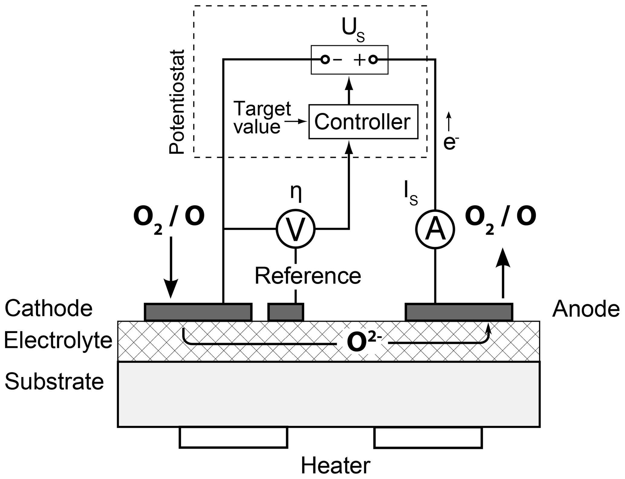
The basic layout of a planar FIPEX sensor is shown in Fig. 1a, while Fig. 2 sketches the single steps that take place in an amperometric sensor. The core is a layer of a ceramic solid electrolyte, commonly yttria-stabilized zirconia (YSZ), an electrical insulator that may transport oxygen anions ${\mathrm{O}}_{\mathrm{2}}^{-}$ due to the structure of its crystal lattice. Metal electrodes applied to the electrolyte serve as electron donors and form an interface at which gas-phase oxygen is reduced in a charge transfer reaction and is subsequently incorporated into vacant lattice sites of the ceramics. This occurs along the so-called triple phase boundary (TPB) at which the electrolyte, electrode and gas phase are in direct contact. Oxygen atoms that have been adsorbed on the electrode have to be transported to this active zone via surface diffusion. In amperometric sensors, a voltage U_S applied between two electrodes creates a gradient in the electrochemical potential of the oxygen anions, which drives them from the cathode to the anode. This results in a net flux of charges through the electrolyte that is coupled with an electronic current in the outer circuit connecting the electrodes. This current is measured as the sensor signal I_S. It depends on the amount of oxygen being delivered along the electrode surface to the triple phase boundary and is thus a function of the ambient oxygen partial pressure.

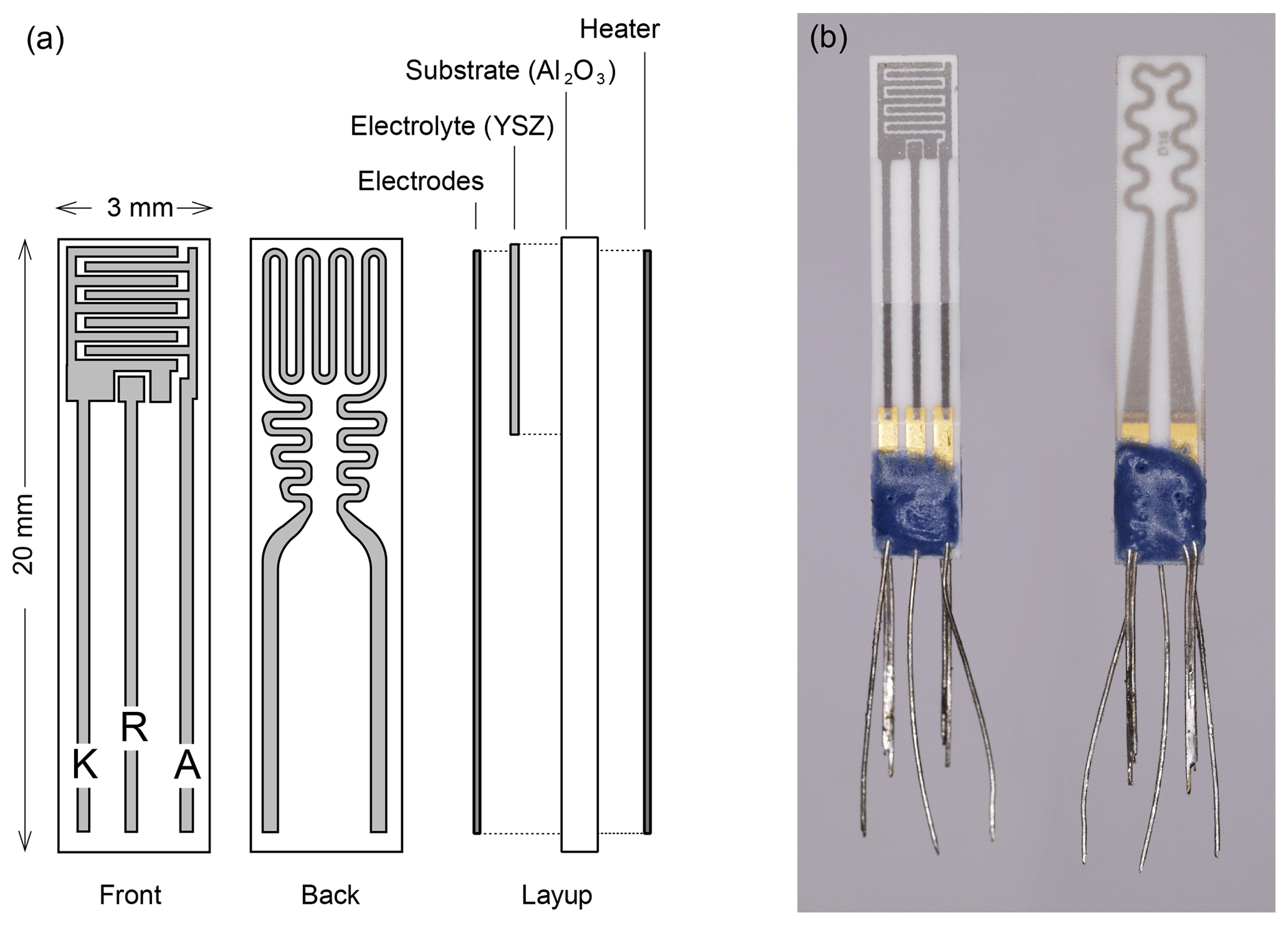
Figure 1 (a) Schematic layout of the three-electrode FIPEX sensors. Front side with interdigitated electrodes, back side with resistance heater. (b) Photo of a screen-printed sensor with platinum electrodes. The leads are sealed with a blue glass layer.

An important factor is the adsorption characteristics of the electrode material. Platinum has the ability to adsorb oxygen molecules dissociatively (Luntz et al., 1988; Lewis and Gomer, 1968; Eichler and Hafner, 1997), which is a requirement for them to be incorporated into the reaction chain. Gold, by contrast, does not show these properties and adsorbs solely gas-phase atomic oxygen (Sault et al., 1986; Canning et al., 1984; Linsmeier and Wanner, 2000) but not O₂ molecules (Eley and Moore, 1978; Canning et al., 1984; Bazhutin et al., 1979). Sensors with platinum electrodes therefore respond to both molecular and atomic oxygen, whereas those having gold electrodes are selectively sensitive to oxygen atoms.

Commonly, a currentless third electrode is employed and the voltage between this reference and the cathode is measured as the so-called cathodic overpotential η. This value is a measure for the deviation of the cathode from its currentless equilibrium condition and defines the working point of the sensor. In order to keep it constant during varying oxygen concentrations a potentiostat is used as an overpotential control, an electronic circuit that regulates the voltage U_S accordingly. Remarkably, this controlling has the effect of significantly accelerating the sensor reaction to pressure changes compared to an operation with a constant voltage U_S (Eberhart, 2018). This transient sensor response is a function of several parameters. In addition to the temperature of the sensor and the mode of operation it also depends on the oxygen density itself, whereby higher pressures lead to a faster sensor reaction. For operation with a potentiostat, experimental results for sensors with platinum electrodes in molecular oxygen indicate response times of the order of a second at pressures in the range of 10⁻⁵ mbar, defined as the time required to reach a sensor signal within 5 % of the stationary level (Eberhart, 2018). For gold electrodes in atomic oxygen, experimental data are limited but show a comparable transient behavior.

The ion conductivity of the electrolyte shows an exponential dependence on temperature (Park and Blumenthal, 1989) and requires the sensors to be heated to approximately 700 K. This temperature has to be stabilized as it directly influences the measurement signal and the sensor characteristics.

Figure 2 Schematic circuit of sensor electrodes.

The technical embodiment of an amperometric solid electrolyte FIPEX sensor is shown in Fig. 1b. The single layers, all of which have been screen-printed, are sketched. On an alumina substrate, a functional YSZ film was printed from a paste. Interdigitated platinum electrodes were applied to this electrolyte layer and a resistance heater attached to the back side of the substrate. For both the electrodes and the heater the same paste was used (Ferro 64120410, Germany). YSZ powder (Tosoh Corporation, Japan) was added to the paste on the electrode side in order to produce a porous layer with an increased triple phase boundary. The electrodes were subsequently electroplated with gold in an electrolyte solution (no. 530522, Dr. Ropertz GmbH, Germany). At the elevated temperatures during sensor operation this formed a stable gold–platinum alloy with the benefit of highly improved adhesion of the metallic layer to the ceramic electrolyte compared to pure gold while preserving the selective adsorption of atomic oxygen (Eberhart, 2018). The electrodes and the heater were contacted with gap-welded Pt–Ni leads.

The sensors were operated on custom-designed electronics during calibration and flight. They controlled the overpotential of the cathode and stabilized the sensor temperature by regulating the resistance of the heater to a constant value. The sensor signal I_S in the range of nano-amperes to microamperes was sampled at 100 Hz and digitized with 16 bit resolution.

3 Calibration

In order to determine the distinct relation between the sensor signal and the atomic oxygen number density a pointwise calibration has been carried out. This is demanding as it involves the production of an exactly metered flux of atomic oxygen and the reliable quantitative detection of this flux by a reference instrument. The setup used is an advance on the method developed for the WADIS-1 campaign (Eberhart et al., 2015) and is sketched in Fig. 3. Atomic oxygen is produced from the dissociation of O₂ in a microwave plasma sustained within a cylindrical quartz tube (5) having an outer diameter of 50 mm and a wall thickness of 2.5 mm. Microwave energy is generated in a magnetron (2.45 GHz, SAIREM, France) with a power of up to 300 W and fed to a resonator (1) that contains the discharge tube. The tube is filled with pure molecular oxygen at a pressure of 1 mbar and is mounted to a high-vacuum chamber (8). The atomic oxygen generated in the discharge is expanded into the vacuum through a small orifice (6) (∅ 0.3 mm) along with undissociated O₂ and forms a fast molecular beam with a distinct radial and axial distribution of the atomic oxygen density. This radial beam profile can be probed by a FIPEX sensor (10) mounted on a linear manipulator (11) (MDC Vacuum Products) and, exploiting the radial symmetry of the beam, by a quadrupole mass spectrometer (9) (QMS; Hiden HAL 3F) on a movable flexible bellow (12) from the opposite side. The QMS is equipped with an electron impact ion source in cross-beam configuration.

There is, however, an important difference between the two instruments. While the QMS measures the static number density of the species (Singh et al., 2000), the sensors determine the particle flux onto their electrodes.

Therefore, a further measurement is required to qualify the mass spectrometer as a reference instrument for moving media. A bubble flowmeter (7) (Sigma-Aldrich) in the feed line of the quartz tube is used to quantify the total mass flow rate of the molecular beam, which is of the order of micrograms per second. Mass continuity requires that the product of the total number flux density $\dot{n}$ in the molecular beam and the local particle mass m, integrated over a solid angle ω of 2π, equals the mass flow rate ${\dot{m}}_{\mathrm{in}}$ in the feed line:

$$\begin{array}{}\text{(1)}& {\dot{m}}_{\mathrm{in}}=\stackrel{\mathrm{2}\mathit{\pi }}{\int }\dot{n}\left(\mathit{\omega }\right)m\left(\mathit{\omega }\right).\mathrm{d}\mathit{\omega }\end{array}$$

For the following it is beneficial to define the partial number flux density ${\mathrm{\Psi }}_i^n$ of species i:

$$\begin{array}{}\text{(2)}& {\mathrm{\Psi }}_i^n={\displaystyle \frac{{\dot{n}}_i}{\sum {\dot{n}}_i}}={\displaystyle \frac{n_i{m}_i^{-\mathrm{1}/\mathrm{2}}}{\sum n_i{m}_i^{-\mathrm{1}/\mathrm{2}}}}\text{with}{\dot{n}}_i=n_i\stackrel{\mathrm{‾}}{c_i}.\end{array}$$

The mean free path of the particles at the operating pressure of around 1 mbar is of the order of the orifice diameter, and it is assumed here that the velocity in the beam is mainly determined by the mean thermal velocity $\stackrel{\mathrm{‾}}{c_i}$ within the discharge tube:

$$\begin{array}{}\text{(3)}& \stackrel{\mathrm{‾}}{c_i}=\sqrt{{\displaystyle \frac{\mathrm{8}{k}_{B}T}{\mathit{\pi }{m}_i}}}.\end{array}$$

Here k_B is the Boltzmann constant. The mean velocity of the particles is thus a function of their mass according to $\stackrel{\mathrm{‾}}{c_i}\propto \mathrm{1}/\sqrt{m_i}$, with the unknown temperature T dropping out in Eq. (2).

The radial distribution of the number densities n_i of the species in the flow is determined by the mass spectrometer, with n_i and the number flux density ${\dot{n}}_i$ being linked by the mean particle velocity $\stackrel{\mathrm{‾}}{c_i}$. Detected species comprise molecular and atomic oxygen and trace amounts of nitric oxide and nitrogen.

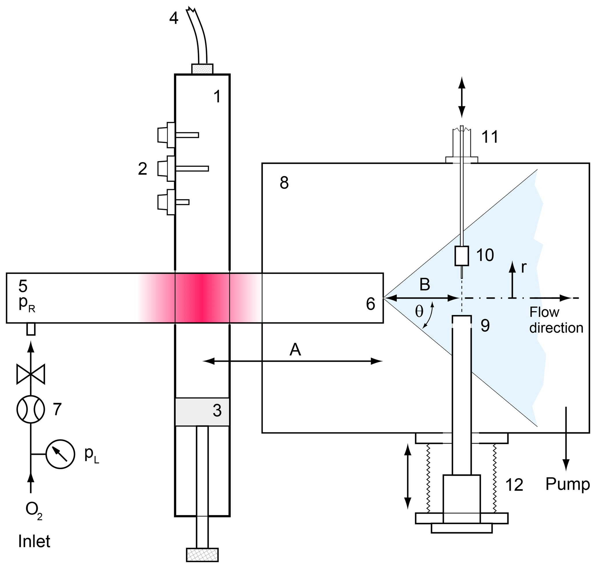
Figure 3 Calibration setup for atomic oxygen. 1 – microwave wave guide, 2∕3 tuner and short circuit for impedance matching, 4 – coaxial line, 5 – fused silica tube, 6 – orifice, 7 – O₂ inlet with bubble flowmeter, 8 – high-vacuum chamber, 9 – mass spectrometer with cross-beam ion source, 10 – solid electrolyte sensor in mounting, 11 – moveable vacuum manipulator, 12 – movable bellows.

The absolute value of the mass flow rate through the orifice is a function of gas temperature (Rugamas et al., 2000). However, it could be shown that the qualitative radial profile of $\dot{n}$ in the molecular beam is identical in the cases of ignited plasma and a cold O₂ flow (Eberhart, 2018). This profile was determined beforehand with the aid of a calibrated O₂ sensor with platinum electrodes and is shown in Fig. 4, plotted over the beam angle θ as sketched in Fig. 3. It is in excellent agreement with a theoretical profile published by Giordmaine and Wang (Giordmaine and Wang, 1960). To account for the finite spatial resolution of the sensor measurement, the theoretical profile has to be convolved with the area of the electrode surface.

This normalized profile is used to calculate the total mass flow rate within the molecular beam that has to equal the measured value in the feed line:

$$\begin{array}{}\text{(4)}& {\dot{m}}_{\mathrm{in}}\equiv \mathrm{2}\mathit{\pi }\underset{\mathrm{0}}{\overset{\mathit{\pi }/\mathrm{2}}{\int }}g\cdot {\dot{n}}_{\mathrm{norm}}\left(\mathit{\theta }\right){\stackrel{\mathrm{‾}}{m}}^{*}\left(\mathit{\theta }\right)\sin \mathit{\theta }\mathrm{d}\mathit{\theta }.\end{array}$$

The linear factor g is found iteratively until Eq. (4) is satisfied, which then yields the radial variation of the species number flux density $\dot{n}\left(\mathit{\theta }\right)=g\cdot {\dot{n}}_{\mathrm{norm}}\left(\mathit{\theta }\right)$. The mean local mass ${\stackrel{\mathrm{‾}}{m}}^{*}$ of the gas mixture in this form has to account for the different velocities of the single species and is calculated as

$$\begin{array}{}\text{(5)}& {\stackrel{\mathrm{‾}}{m}}^{*}=\sum _i{\mathrm{\Psi }}_i^n{m}_i.\end{array}$$

The desired distribution of the atomic oxygen number flux density ${\dot{n}}_{\mathrm{O}}$ can finally be calculated as

$$\begin{array}{}\text{(6)}& {\dot{n}}_{\mathrm{O}}\left(\mathit{\theta }\right)=\dot{n}\left(\mathit{\theta }\right){\mathrm{\Psi }}_{\mathrm{O}}^n.\end{array}$$

Subsequently, the sensor signals are evaluated at corresponding positions in the beam, defined by the angle θ or the radial coordinate r as sketched in Fig. 3.

All calibration steps can be done within one and the same experiment with the plasma running continuously. The result is the sensor signal I_S as a function of the atomic oxygen number flux density. In a medium at rest, this flux density onto a surface can be related to the ambient number density under the assumption of a Maxwellian velocity distribution (Frohn, 1988):

$$\begin{array}{}\text{(7)}& n=\dot{n}{\displaystyle \frac{\mathrm{4}}{\stackrel{\mathrm{‾}}{c}}}.\end{array}$$

The relation between I_S and n_O then serves as a calibration curve that assigns atomic oxygen number densities to the sensor signals recorded along the trajectory. The mean velocity $\stackrel{\mathrm{‾}}{c}$ is a function of temperature, so the calibration is valid for a given reference temperature. For the evaluation of flight data, the local ambient temperature has to be taken into account, which can be derived from the CONE results.

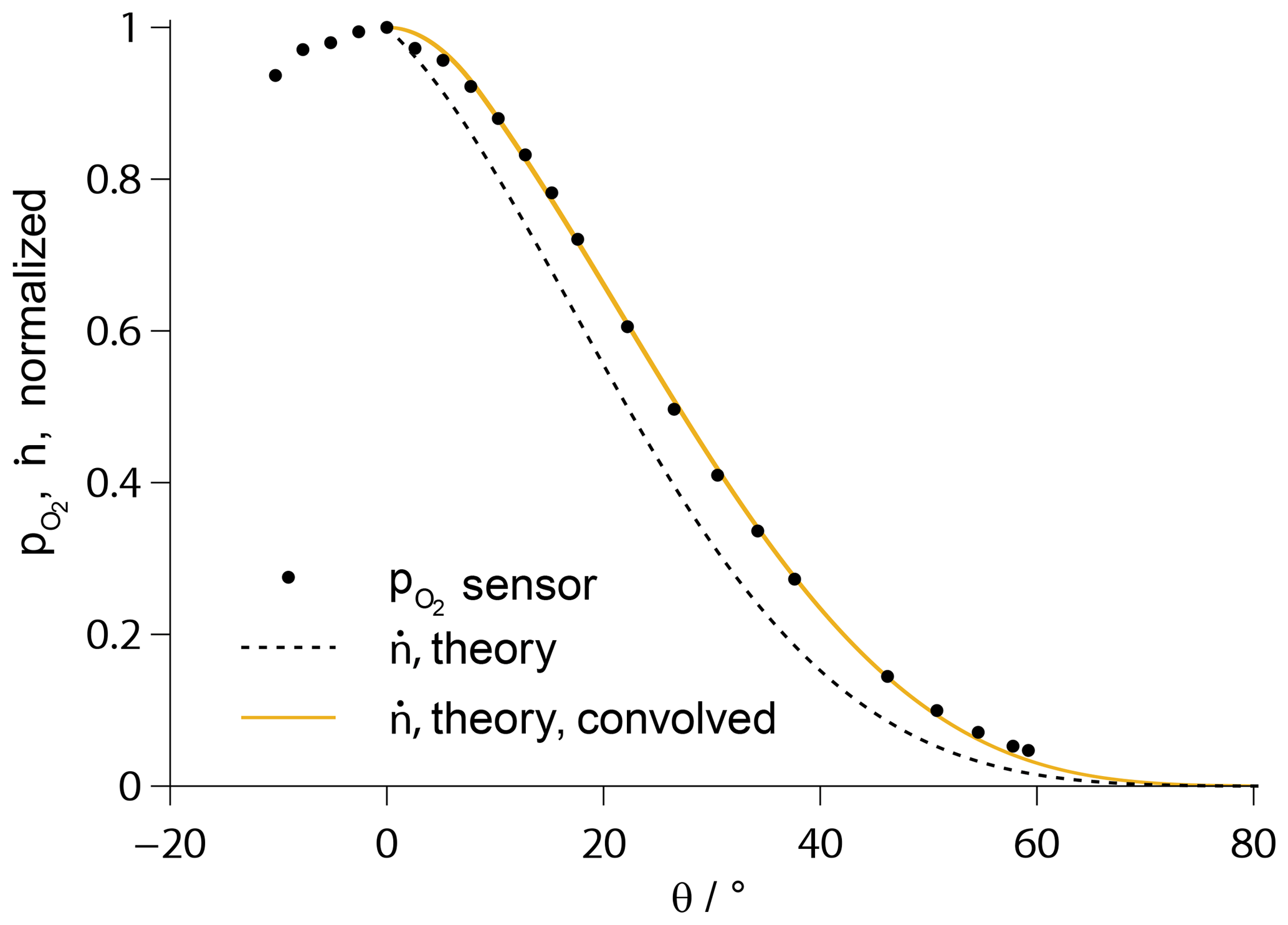
Figure 4 Theoretical profile of the number flux density according to Giordmaine and Wang (1960), convolved with the electrode length and fitted to the measurement data of a platinum sensor (solid line). The profile prior to convolution is additionally given (broken line).

In mass spectra measured by a QMS spurious signals at mass number 16, attributed to atomic oxygen, can be generated by the dissociative ionization of O₂ or due to doubly ionized oxygen molecules. In order to suppress these contributions, the ion source was tuned to a very low electron energy of 16 eV, which is below the dissociation threshold of O₂ but above the appearance potential of atomic oxygen. This practice in turn requires a calibration of the QMS as it is operated with nonstandard settings. For this purpose, the spectrometer reading for the different gases was recorded against a precise capacitative high-vacuum-pressure gauge (MKS Baratron 619A). In the case of atomic oxygen, a method based on methane (CH₄) with the identical mass number 16 was employed (Agarwal et al., 2004). The energy scale of the ionizer was calibrated using the well-known appearance potential of argon. As the electrical fields of the microwave discharge may affect the potentials within the ion source, this energy calibration was done with the plasma running.

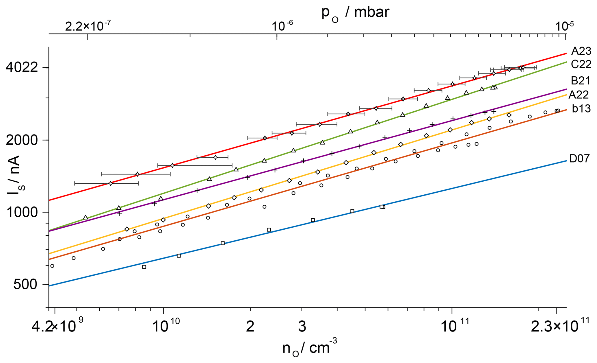
Figure 5 Calibration curves for atomic oxygen for sensors used on the WADIS-2 campaign in double-logarithmic plotting for a reference temperature of 293 K. Solid lines represent power functions fitted to the measurement data. The uncertainty of the calibration is given exemplarily for sensor A23, with the standard deviation of I_S below 10 nA.

The characteristics of single sensors vary slightly due to manufacturing tolerances. This affects, e.g., the position of the electrodes relative to the heater, the porosity of the electrodes or the gold plating and requires an individual calibration. The results for all sensors on WADIS-2 are in Fig. 5 in a double-logarithmic presentation for a reference temperature of 293 K. The lower abscissa shows atomic oxygen number densities, while the upper abscissa gives the corresponding partial pressures. Power functions of the type $I_{\mathrm{S}}=\mathit{\alpha }\cdot n_{\mathrm{O}}^{\mathit{\beta }}$ have been fitted to the measured points and appear here as straight lines. The parameter β is a characteristic of the limiting reaction mechanism at the electrodes. It is close to 0.35 for all tested sensors, while the value of the sensitivity parameter α varies. Error bars are shown exemplarily for sensor A23. They represent the uncertainty of the calibration that is detailed in Appendix A. It amounts to a maximum of $+\mathrm{35}/-\mathrm{28}$ %.

With the described calibration method 2 orders of magnitude in the number density of atomic oxygen could be covered, spanning 10⁹ to 10¹¹ cm⁻³. This density range is typically expected in the MLT region and allows for the analysis of the sensor signals measured along the trajectory without the requirement of extrapolating the calibration curves.

During calibration, all sensors were mounted in the same heads that were used on the rocket flight as shown in Fig. 6. They were controlled by the same electronics and were connected using the actual flight hardware.

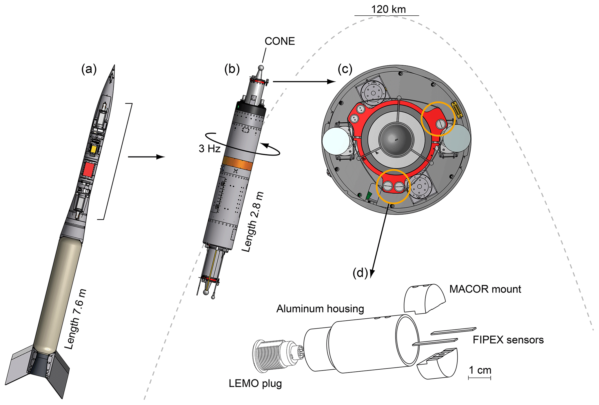
Figure 6 Rocket configuration of the WADIS mission. (a) Total view including motor and nose cone. (b) Spin-stabilized payload with instrument decks on the fore and aft and sketched trajectory. (c) Details of the foredeck with highlighted positions of the FIPEX sensor heads. (d) Assembly of a sensor head with two sensors mounted in an aluminum housing.

4 Rocket experiment

WADIS-2 was launched on 5 March 2015 at 01:44 UTC from Andøya Space Center in northern Norway (69^∘ N, 16^∘ E). The configuration of the rocket is sketched in Fig. 6a. A single-stage VS-30 motor propelled the payload shown in panel (b) to an apogee of 120 km. Instrument decks were both fore and aft of the payload and were symmetrically equipped with FIPEX sensors and the central CONE instrument.

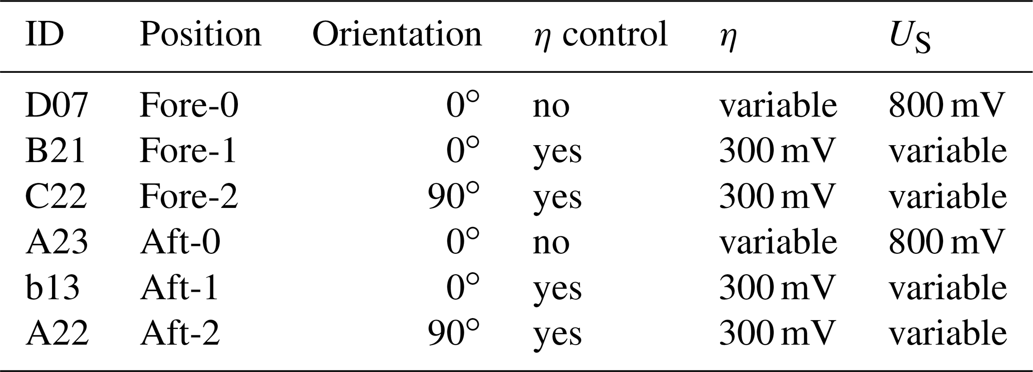
The payload was spin-stabilized with a rotational speed of about 3 Hz and kept a constant orientation along the trajectory. Panel (c) of the figure gives a detailed view of the foredeck and highlights the position of the sensor heads mounted on a circular adapter ring. An internal view of the heads is shown in panel (d): two FIPEX sensors, one with platinum and one with gold electrodes, were held by a ceramic inset and mounted in a common aluminum housing. The sensitive electrode surface of the sensors was oriented radially outward. In addition to this standard orientation a second type of head was used with the sensors rotated such that the surface normal of the electrodes was parallel to the payload axis. Figure 7 shows a photo of this layout. This variation in sensor orientation was chosen in order to explore the influence of the cross-flow on the measurement results. In a third modification, sensors in the standard orientation were operated with a fixed voltage U_S across anode and cathode. This is in contrast to the normal mode of operation with a controlled overpotential η and should help in investigating the effect of different sensor dynamics on the temporal and spatial resolution of the measurements. On each foredeck and aft deck these three types of sensors were operated in parallel. Table 1 provides an overview.

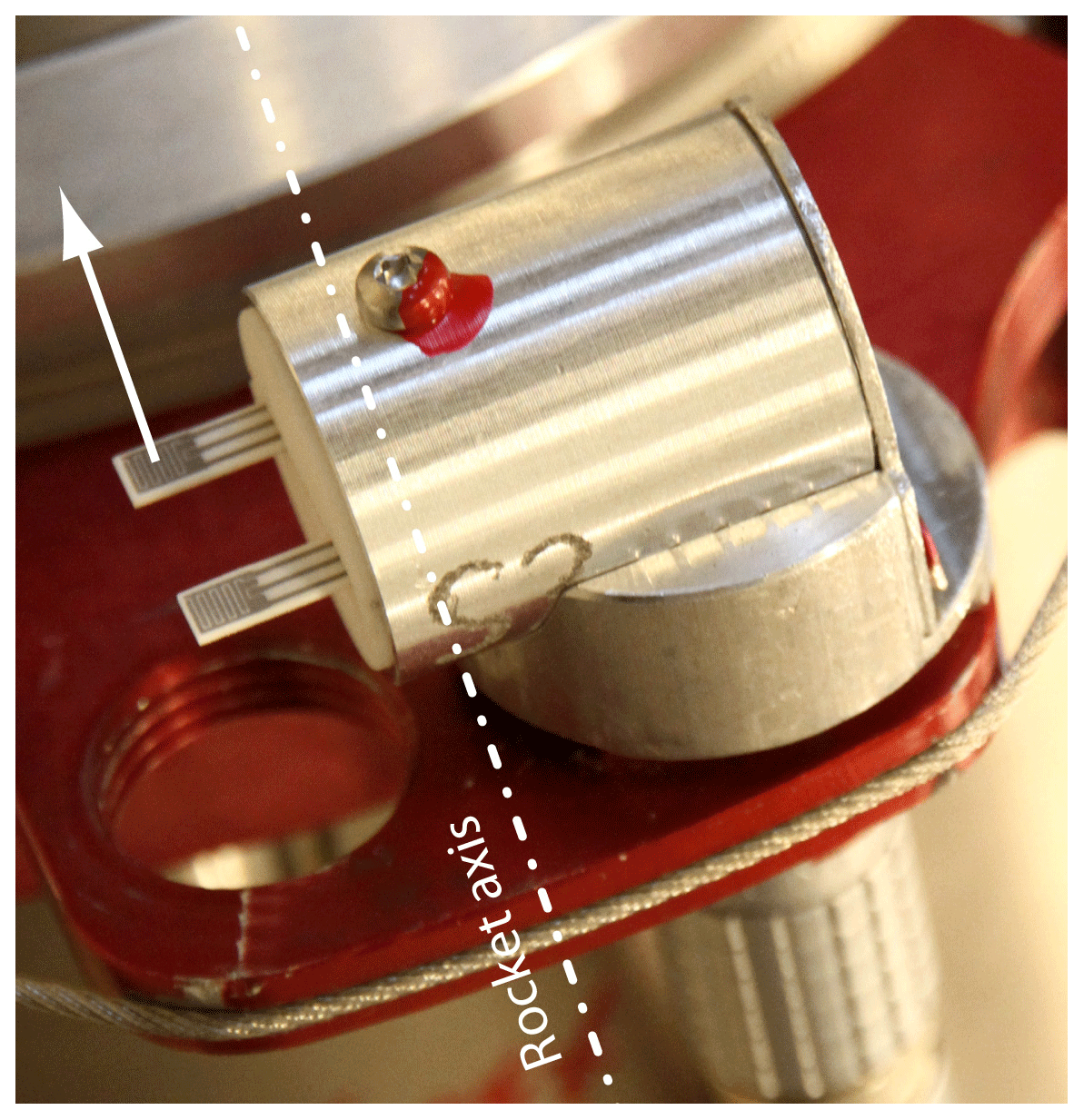
Figure 7 Modified sensor head with orientation of the electrode surface perpendicular to the payload axis.

Table 1 Overview of the sensors measuring atomic oxygen on WADIS-2. Orientation is defined between electrode surface and payload axis.

4.1 Aerodynamic simulation

In order to derive atmospheric number densities from the sensor data, a thorough investigation of the flow field around the rocket structure is inevitable. Aerodynamic effects in the vicinity of the payload cause a deviation of local air properties from their undisturbed values. This affects the density as well as the gas composition that may change through chemical reactions in the shock front or due to mass-dependent reflection at the walls (Bird, 1988).

Numerical simulations of the aerodynamics were conducted in full 3-D with the code PICLas, a direct-simulation Monte Carlo method developed in collaboration between IRS and the Institute of Aerodynamics and Gas Dynamics (IAG) (Munz et al., 2014; Eberhart et al., 2015). The computational grid comprised the complete payload, with the sensor heads modeled as simplified block-like structures. In order to represent the payload rotation due to the spin-stabilized flight mode, one sensor head was included on each of the extreme positions in the windward and the lee of the cross-flow. Figure 9 shows a cutout of the geometries of the grid. Simulations were done at several points of the trajectory, with input parameters taken from GPS data (velocity vector), CONE results (total number density and temperature) and the MSIS-E-90 model (gas composition). This results in aerodynamic correction factors that represent the ratio between the local number density at the sensor position and the value of the undisturbed free stream. These factors have to be applied to the local densities derived from the sensor data. They are given in Fig. 8a as a function of altitude, with ram factors for sensor positions in the compressed region behind the shock front and wake factors representing the rarefied flow at the opposite end of the payload. All factors were evaluated for sensors in their windward position during a payload revolution. Compared to WADIS-1 (Eberhart et al., 2015) the numerical data had to be analyzed at a slightly different location due to modified sensor heads.

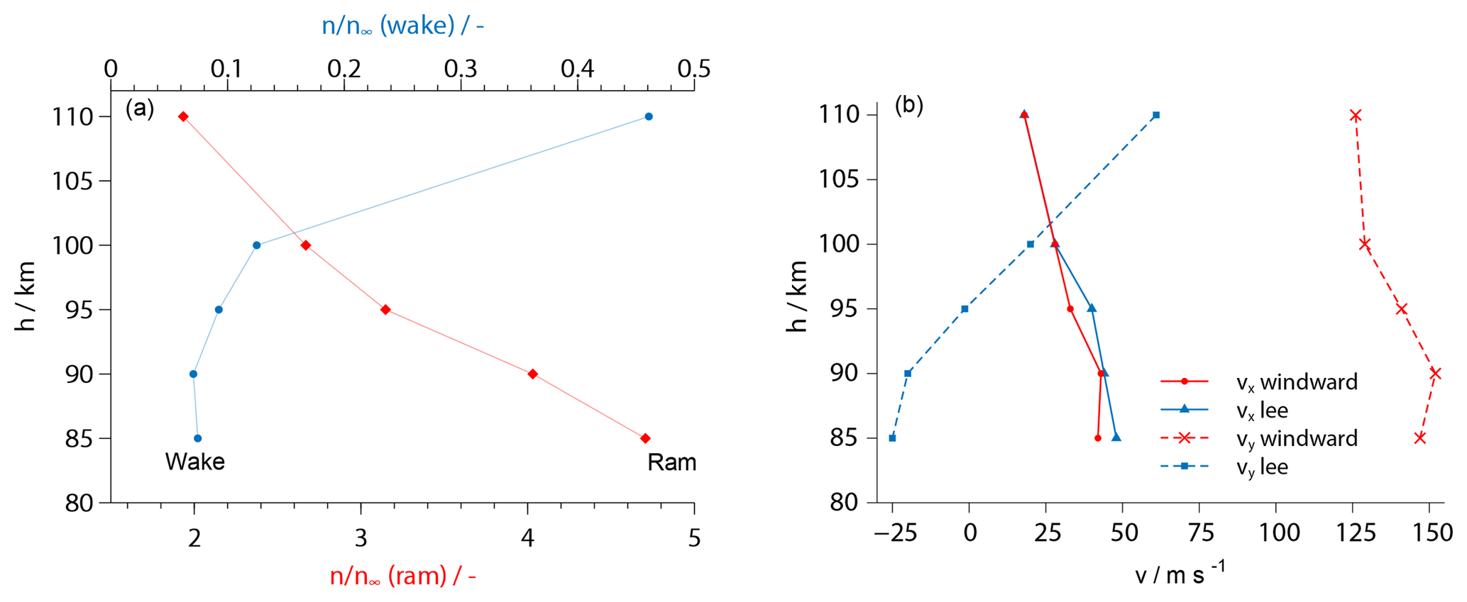
Figure 8 (a) Aerodynamic correction factors for sensors in ram and wake position derived from numerical simulations at the windward side. Each dot represents a calculated trajectory point. (b) Longitudinal (x) and lateral (y) velocity components at the sensor position, calculated in ram.

As the FIPEX sensors do not measure the number density n directly but determine the particle flux $\dot{n}$ onto the sensitive electrode surface, it is furthermore important to consider the local flow velocities in the data analysis:

$$\begin{array}{}\text{(8)}& \dot{n}=n({\displaystyle \frac{\stackrel{\mathrm{‾}}{c}}{\mathrm{4}}}+v_n).\end{array}$$

Here the first term on the right-hand side represents the flux density caused by a medium at rest with a Maxwellian velocity distribution and a mean speed $\stackrel{\mathrm{‾}}{c}$. The second term is the contribution due to a directed velocity v_n oriented perpendicular to the surface.

Figure 9 presents numerical results for a trajectory point at 85 km of altitude. In panel (a), the colors indicate the longitudinal velocity v_x, with the cross-flow component v_y in panel (b). The actual sensor position and the standard orientation of the electrode surface are marked by red arrows. It is remarkable that the value of v_x is almost constant at around 40 m s⁻¹ during a rotation period, whereas v_y greatly differs when comparing the windward and the lee position. This aspect will be important in the discussion of the absolute number densities derived from the sensor data. Figure 8b plots the simulated velocity components, calculated for the ram side of the payload, as a function of altitude.

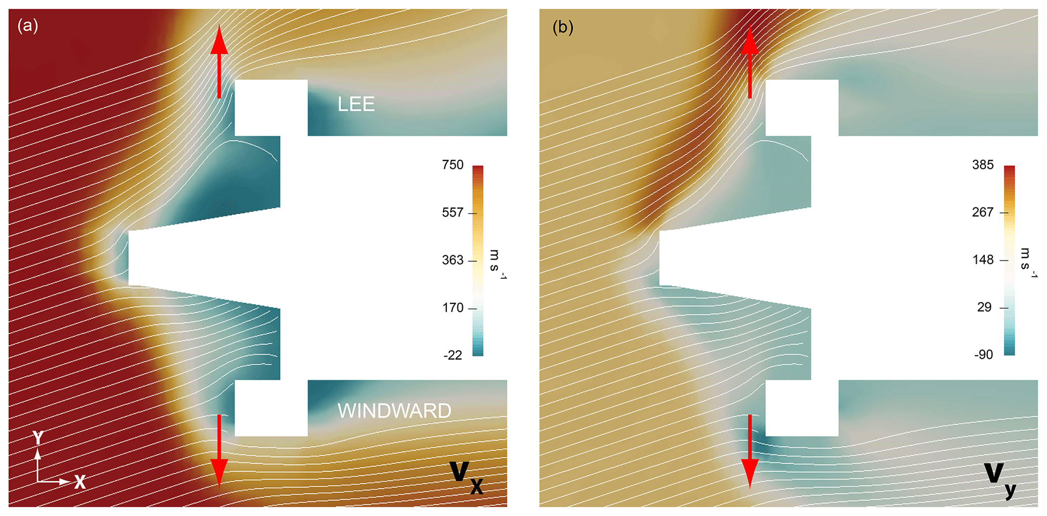
Figure 9 Numerical results of an aerodynamic simulation of the payload at a trajectory point at 85 km of altitude during downleg. Colors indicate the components of the velocity vector. (a) Longitudinal (x), (b) lateral (y). Red arrows mark the sensor position and the orientation of the electrode surface.

4.2 Results

The raw signals of the sensors are formed by the temporally measured currents between their electrodes. Figure 10a shows a section with a length of about 10 s. Clearly visible are periodic oscillations with large amplitudes due to the rotation of the payload. During one revolution, the sensors travel through regions with different aerodynamic conditions, showing maxima and minima of the local density on the windward and leeward sides with respect to the cross-flow. A frequency analysis of the signals, given in panel (b), reveals pronounced peaks at the nominal rotational frequency of about 3.3 Hz and their harmonics. These frequencies may be suppressed by notch filters with a small bandwidth. The central red line in panel (a) shows the result of such a filtering.

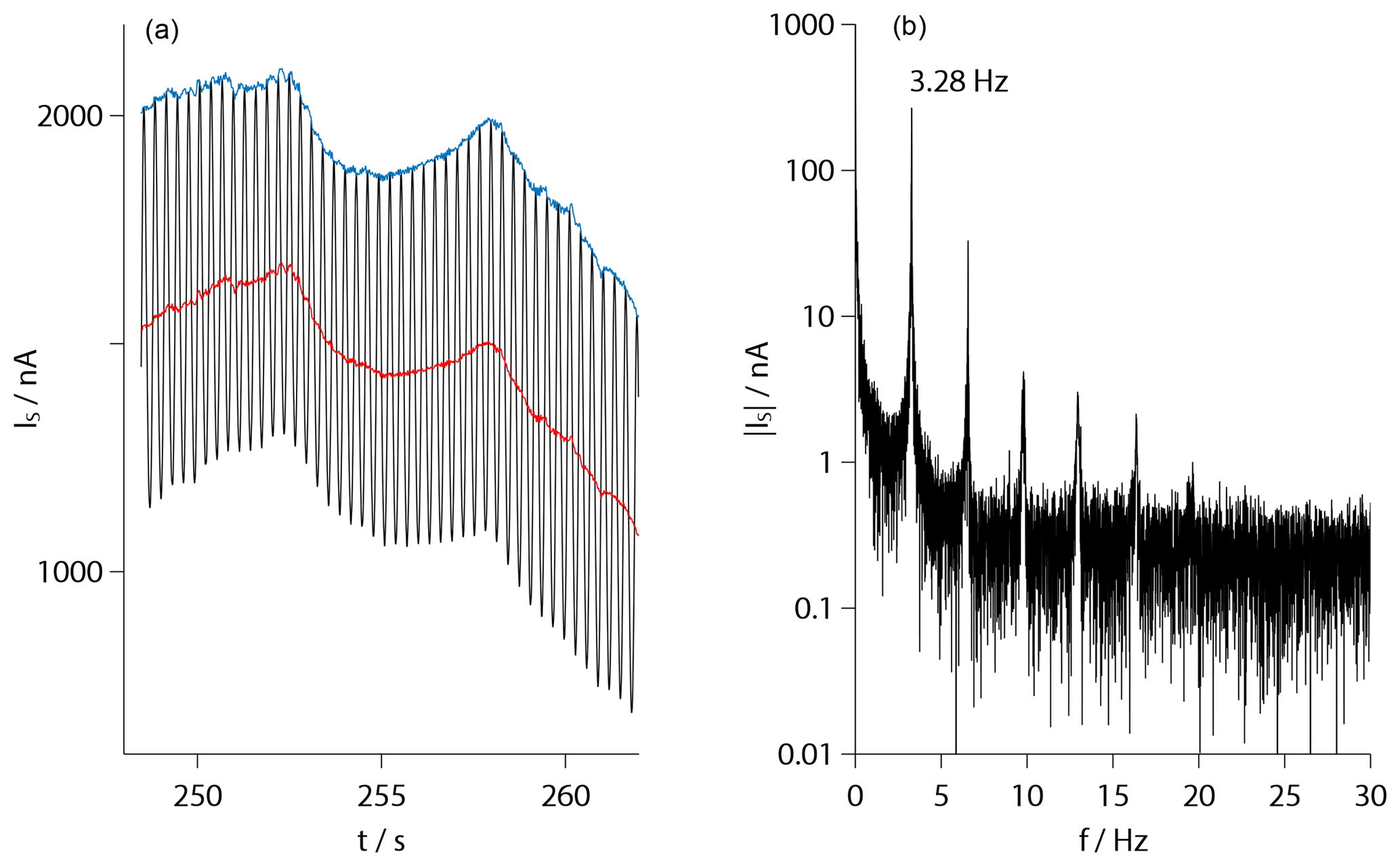
Figure 10 (a) Detail of the transient sensor signal showing periodical oscillations due to the payload rotation. The red curve is the result of a filtering by several narrow-bandwidth notch filters, and the blue curve is obtained by subsequent fitting to the maximums. (b) Frequency spectrum of the raw signal with clear peaks at the rotational frequency and its harmonics.

In order to determine number densities, the individual calibration curves of the sensors and the appropriate aerodynamic corrections have to be applied to the raw data. However, the ram and wake factors given in Fig. 8 have been determined for the condition in the windward region so that their direct application to the filtered data would underestimate the number density. The analysis involves an additional step: the filtered data are shifted such that they coincide with the maxima of the raw data at their common time points. This is based on the assumption that the maxima in the signal level coincide with the maxima of the oxygen density, which may be a simplification due to the transient behavior of the sensors. Figure 10a shows the result of this operation given by the upper blue line.

According to Eq. (7) the local flow velocity v_n perpendicular to the sensor surface additionally has to be taken into account. For the sensors in standard orientation, this is equivalent to the velocity component v_y given in Fig. 9b, which is close to zero in the windward region and can be approximately neglected. For the rotated sensors, on the other hand, the component v_x shown in Fig. 9a is relevant with an altitude-dependent value of around 100  m s⁻¹. Both the ram and wake factors and the local flow speeds are interpolated linearly at altitudes between the simulated trajectory points. According to Eq. (7), the calibration curves given in Fig. 5 are valid for a defined reference temperature, and their correct application requires knowledge about the local temperature in the atmosphere. These data can be evaluated from the CONE measurements along the trajectory.

Due to the common time base of the sensor electronics and the onboard GPS receiver, the determined number densities of atomic oxygen can be plotted as a function of altitude upleg and downleg of the flight path. Given the sensor sampling rate of 100 Hz and the evolution of the payload velocity, the nominal spatial resolution in the vertical direction is better than 10 m during the experimental phase.

4.2.1 Upleg

Vertical profiles of the number densities n_O of atomic oxygen determined during the upleg are given in Fig. 11. Results from all six employed sensors, including aerodynamic corrections, are sketched in individual lines. During this phase, the sensors on the foredeck were located in the ram, whereas the aft sensors measured in the wake of the payload. As a reference, the values derived from the upleg photometer data and a profile taken from the NRLMSIS-00 atmospheric model are additionally drawn and for the sake of clarity scaled by a factor of 0.25. The photometer data are based on measuring the emission in the atmospheric band of molecular oxygen at 762 nm and yield a reliable quantitative density profile that is most accurate between 87 and 96 km of altitude (Hedin et al., 2009). Above and below that region the analysis is challenged by unsteady auroral emissions as recorded by a dedicated onboard auroral photometer. This leads to O densities that are higher than expected.

Figure 11a shows the data in a linear plot, whereas panel (b) uses a semilogarithmic representation. The results from the individual sensors are both qualitatively and quantitatively nonuniform. The values from the aft sensors are very low and begin to rise only above 97 km, while sensor no. 2 remains at zero throughout the upleg. On the foredeck, the sensors with controlled overpotential (no. 1 and 2) show a sharp peak at around 83 km before the signal drops. Of these two, only sensor no. 1 rises again significantly above 92 km and develops a maximum at around the same height as the NRLMSIS model. The values from the uncontrolled fore sensor no. 0 rise rather gradually above 80 km, with a maximum at around 101 km, which is close to the peak of Aft-0. The shading around the profile of sensor Fore-0 illustrates the maximum uncertainty of the calibration of $+\mathrm{35}/-\mathrm{28}$ %.

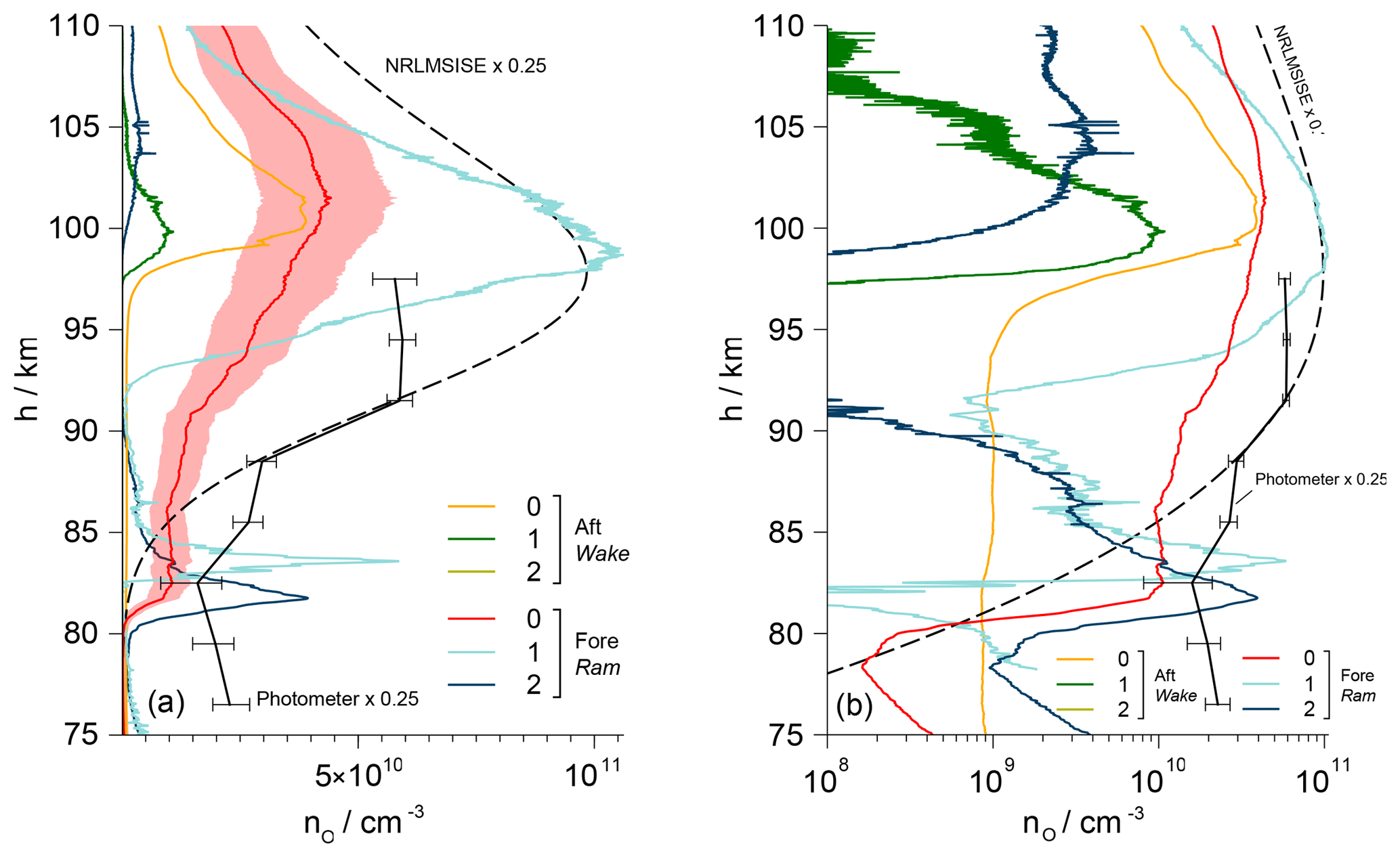
Figure 11 (a) Vertical profile of the atomic oxygen number density along the upleg of WADIS-2 including aerodynamic corrections. Fore sensors are in ram, aft sensors in wake. Values of Aft-2 are all zero. The shading around the profile of sensor Fore-0 indicates the uncertainty of the calibration. The scaled profiles derived from the onboard airglow photometer data and the NRLMSISE-00 atmospheric model are sketched for comparison. (b) Semilogarithmic plotting.

4.3 Downleg

Figure 12 summarizes the results from the individual sensors on the downleg of the trajectory. During this flight phase the aft sensors measured in the ram position, and the fore sensors stayed in the wake. Again, Fig. 12a presents the data in a linear plot and panel (b) in a semilogarithmic diagram. The results are complemented by a curve plotted from the downleg photometer results and a profile from the NRLMSIS-00 model. Again, the photometer data suffer from unsteady auroral emissions below approximately 87 km.

In contrast to the data acquired during the upleg, the vertical profiles of atomic oxygen number densities are now obviously more uniform, including the comparison between fore and aft sensors. The values of sensor Aft-2 are more than an order of magnitude higher than those of the other sensors and are in good agreement with the photometer data and the NRLMSIS model. The reason for this quantitative deviation is the rotated orientation of this sensor and the associated aerodynamic conditions. Profiles from the aft sensors no. 0 and no. 1 in standard orientation are very close to each other in both qualitative and absolute measures. During the downleg, sensors on the foredeck of the payload were positioned in a region of rarefied flow so that a correction using the wake factors from Fig. 8 will raise the number densities. This is obvious from the increased noise level in the profile of the rotated sensor Fore-2. In the wake, the particle velocity is less directed than in the ram. The sensor orientation plays a minor role here and the results agree well with those of Fore-0 in standard orientation. Both profiles show clear similarity to the atmospheric model, with absolute values lower by 50 %. The reduced noise level of Fore-0 is a result of the sensor operation without an overpotential control. The very low values of Fore-1 are noticeable, while its relative variation is in agreement with the other sensors. The cause of this difference in signal level cannot be unambiguously identified. Supposedly, the reason is an increased sensitivity of this sensor to molecular oxygen that was found during the calibration procedure. This may be due to an uneven gold plating of the electrodes that affects the sensor reaction via the overpotential control. As a result, the signal may be pushed during a phase of decreasing O₂ concentration on the upleg as well as lowering it during an increase during downleg. In this regard the comparatively high signal during the upleg, shown in Fig. 11, could also be interpreted as an overshooting based on this effect. A very careful and even plating of all electrodes with gold is therefore an important requirement and should be checked rigorously during calibration.

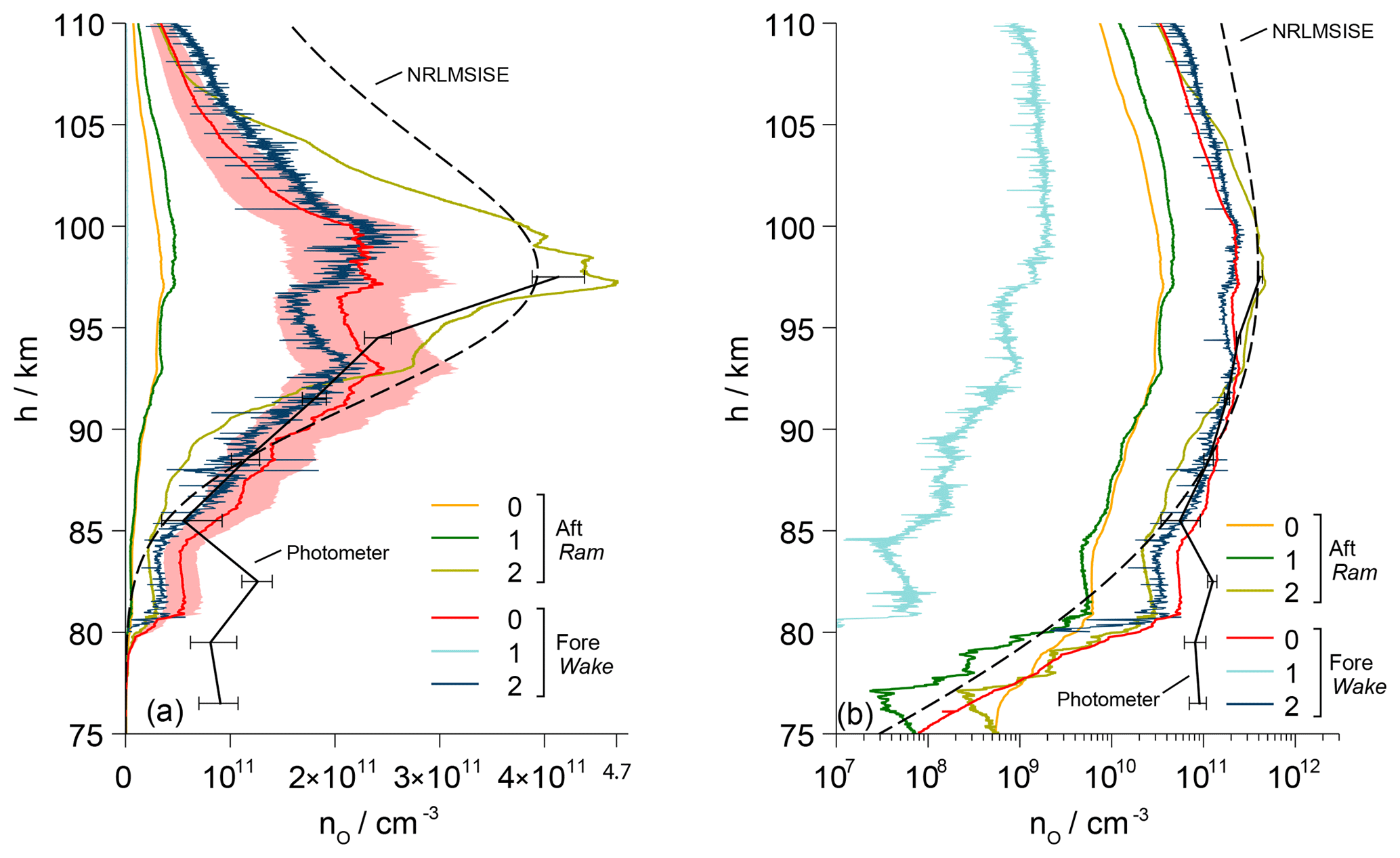
Figure 12 (a) Vertical profile of the atomic oxygen number density along the downleg of WADIS-2 including aerodynamic corrections. Aft sensors are in ram, fore sensors in wake. The low values of Fore-1 are not resolved here. The shading around the profile of sensor Fore-0 indicates the uncertainty of the calibration. The profiles derived from the onboard airglow photometer data and the NRLMSISE-00 atmospheric model are sketched for comparison. (b) Semilogarithmic plotting.

5 Discussion

Obviously, the measurements of the individual sensors result in individual density profiles that differ quantitatively. This is due to the fact that the sensors were not redundant: as shown in Table 1, all sensors differed in their position (aft or fore), their orientation and their mode of operation. Comparison and discussion of the different results will lead to the identification of the best parameters for a quantitative measurement along the trajectory.

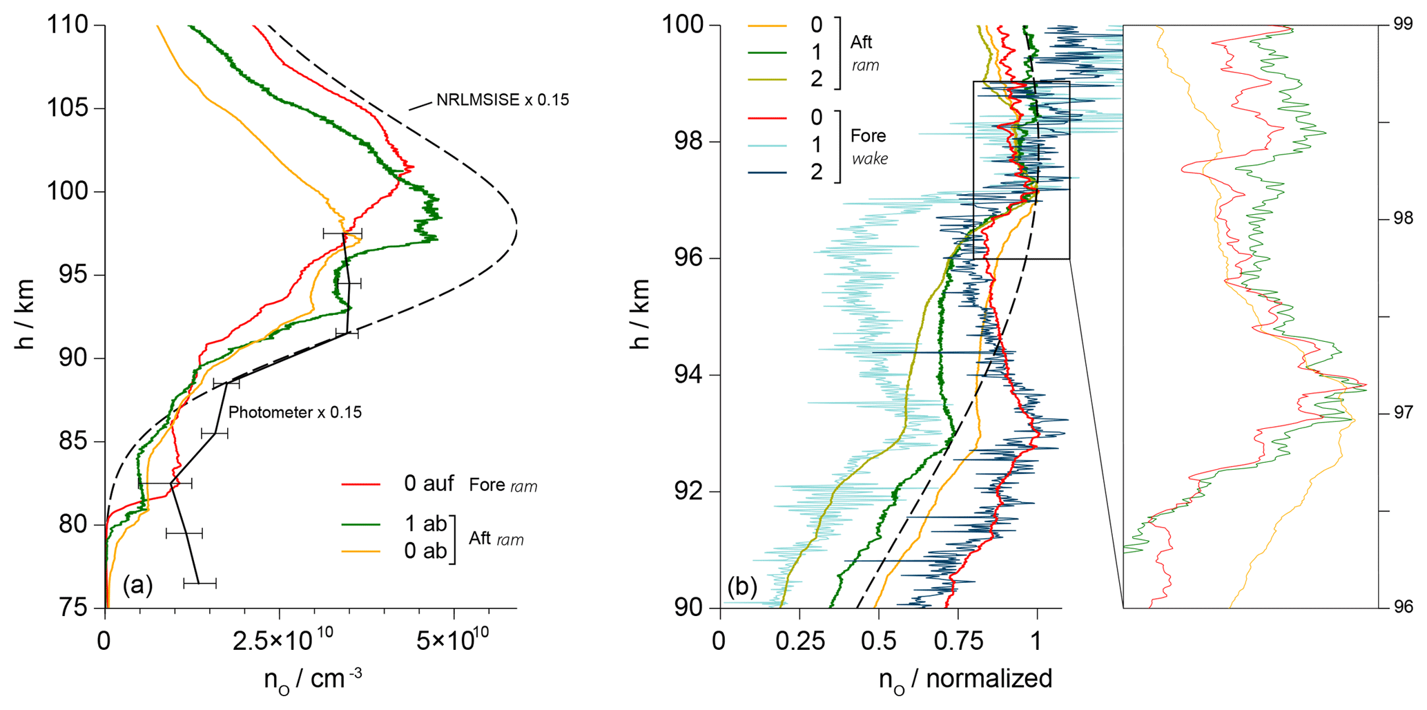
Figure 13 (a) Comparison of the ram profiles of different sensors measured by Fore-0 during the upleg as well as by Aft-0 and Aft-1 during the downleg. Profile derived from the photometer data and values of the NRLMSISE-00 atmospheric model are scaled by a factor of 0.15. (b) Normalized profiles of all sensors during the downleg, with fore sensors in wake and aft sensors in ram position. The inset shows a detail of the profiles featuring small-scale variations.

The resulting profiles measured during the downleg of the trajectory are in considerably better agreement with each other than those of the upleg. This holds for comparisons of sensors within an instrument deck as well as between sensors on the fore and aft. In the initial phase after the separation of the motor and nose cone, a very unstable and nonuniform response of all sensors is observed. This behavior was already found in the data of WADIS-1 (Eberhart et al., 2015) and is the result of a slow accommodation to the high-vacuum environment in the upper atmosphere. Before launch, the sensors were operated for several minutes under ambient conditions. Here sufficient molecular oxygen is adsorbed even on the gold electrodes to maintain a signal level at the upper detection limit of the electronics. Within a very short period after the launch the oxygen concentration drops several orders of magnitude and a certain time is required to reach a new and stable equilibrium between adsorption and desorption at the electrode surface. The interplay of the overpotential control and potentially slightly varying material properties of the electrodes further slows down this process. On both fore and aft the uncontrolled sensors in Fig. 11 end more quickly in a stable condition.

The profile determined in the ram phase during the downleg by sensor Aft-2, mounted in the rotated orientation as illustrated in Fig. 7, is in good agreement with the results of the photometer measurements on the same payload. The analysis of the data includes consideration of the local flow velocities in Eq. (8) in addition to the aerodynamic correction factors given in Fig. 8. The matching results are an indication for the correct calibration of the sensors and for a numerical simulation successfully representing the aerodynamic conditions.

Figure 13a combines three individual results measured in ram positions with a scaled profile derived from the photometer data and an NRLMSIS profile: sensor Fore-0 during the upleg and the aft sensors no. 0 and 1 during the downleg. The absolute values are lower than the atmospheric model, but the profiles agree well on a qualitative basis. The cause of the reduced level of the measurements can be found in the interplay of the transient sensor response and the 3 Hz rotation of the spin-stabilized payload. As illustrated in Figs. 9 and 10, the sensors travel through regions of different densities and varying aerodynamic conditions on the windward and lee side during one revolution. In the lee phase, the sensors in standard orientation encounter a high cross-flow velocity v_y directed away from the electrodes, which greatly reduces the particle flux onto their surface. The slow kinetics of the gold electrodes, with response times assumed in the range of a second, prevent a complete recovery of the signal amplitude on the windward side and lead to reduced number density results. In contrast to that, the longitudinal velocity v_x, relevant to the sensors with rotated orientation, is almost constant during a rotation period. This favorable orientation thus avoids the negative effect of the lee side aerodynamics, and the increased particle flux due to the high v_x velocity reduces the response time of the sensors.

As the fore and aft sensor profiles in Fig. 13a have been measured on opposite sides of the apogee they are separated by a horizontal distance that spans 52 km at 70 km of altitude. One of the goals of the WADIS mission is the investigation of the horizontal variability of the atmosphere. It can be observed, e.g., regarding the dent in the downleg profile of the aft sensors at around 95 km, which is not present during the upleg. The source of this dent with a vertical extent of about 4 km could be a gravity wave with a short period.

Figure 13b is a compilation of the individual downleg profiles, normalized to their respective maxima. Obviously, the results from all six sensors are comparable on a qualitative basis, despite their varying orientation, mode of operation and position on the instrument deck. The diverse course of the profiles between the two maxima at 93 and 97 km of altitude may be due to a differing transient reaction of the individual sensors. As outlined in Sect. 2, an active control of the overpotential η leads to a significant decrease in the response time compared to the uncontrolled operation with a fixed voltage U_S. The comparison of the profiles measured by the aft sensors no. 0 and 1 shows that the dip between the maxima is shallower for the uncontrolled Aft-0, which might give a hint for the significance of this effect. The inset in Fig. 13b gives a zoomed-in cutout of the profiles from three sensors, resolving small-scale signal variations. Apart from a certain noise level, these variations are present in the results from all sensors and occur at identical altitude positions regardless of the mounting position of the sensors, which introduces a phase shift of the raw signals due to the payload rotation. This leads to the conclusion that here actual density variations of atomic oxygen are caught on a very small scale. In line with the discussion above the amplitudes of the variations are smaller for the uncontrolled sensor Aft-0 compared to Aft-1.

Even for sensors with a slow transient response, fast density variations are still represented in the measurements. This holds true up to a certain frequency limit. However, the amplitude of the signals is damped and the absolute value of the density is not resolved correctly. The analysis of the frequency content of the signals nevertheless allows for valuable conclusions on the interaction of atmospheric turbulence and atomic oxygen, which is detailed in a companion paper (Strelnikov et al., 2019).

It is interesting to deal with the question of whether, given the known transient reaction of a sensor, the true amplitude of the density variations could be recovered from the measurements. In the case in which the signal can be represented by a convolution of the transient course of the density with the impulse response of the sensor, so-called deconvolution methods could be used to address this problem. The impulse response can, in principle, be determined experimentally.

Here two fundamental difficulties arise when working with FIPEX sensors: firstly, the transient reaction depends on the density itself. Even though there are techniques that take such varying impulse responses into account, the overall complexity of the analysis increases considerably (Löhle et al., 2013). Secondly, the system under consideration has to be linear so that the course of the signal can be modeled by a convolution operation. Unfortunately, the calibration curve of the sensors, i.e., the dependence of the signals on the density given in Fig. 5, is nonlinear so that a deconvolution of the measurement results would not lead to the desired reconstruction. As a result, the determination of the absolute amplitudes of high-frequency density fluctuations requires the development of fast-response sensors. Investigation of the transient behavior of amperometric solid electrolyte sensors under high-vacuum conditions is part of ongoing research and shall serve to assess the deviation of the measured absolute values as a function of frequency (Eberhart, 2018).

6 Conclusions

Compared to WADIS-1, the newly developed calibration method features a wider density range that can be covered and achieves a better accuracy by directly measuring the mass flow in the molecular beam that the sensors are exposed to. The data analysis now includes consideration of the local flow velocities at the sensor position on the basis of numerical simulations of the payload aerodynamics.

Concerning the design of the sensors, the selective detection of atomic oxygen requires all gold electrodes in order to rule out the influence of molecular oxygen on the measurement via the overpotential control. This also helps in reducing the cross-sensitivity towards other gases that may undergo reactions on catalytically active platinum electrodes and thus falsify the results.

The use of a set of six sensors with different mounting position, orientation and mode of operation enabled the assessment of the sensor performance based on these parameters. The analysis of the density profiles on WADIS-2 yields a preferential sensor orientation with the normal of the electrode surface being parallel to the rocket axis. It is beneficial here that the longitudinal velocity at the sensor position is approximately constant during one revolution of the payload. In contrast, sensors with their electrode surface pointing radially outwards are subject to the cross-flow that largely varies from the windward to the leeward side. The interplay of the payload spin with a comparably slow sensor reaction may lead to a distortion of the absolute results.

The active control of the overpotential of the sensors was found to be beneficial in terms of the transient response compared to the operation with a fixed voltage between cathode and anode.

Shortly after launch, the sensors encounter an initially instable phase after being exposed to the flow, which complicates the measurements during the upleg. The most reliable results are thus obtained during the downleg after the sensors have accommodated the low-density conditions.

The improved calibration procedure and the optimized sensor orientation in conjunction with a detailed aerodynamic analysis now result in a quantitative profile of atomic oxygen number densities in the MLT region with a very high vertical resolution. This profile, measured during the downleg by the sensor Aft-2, is in good agreement with results from the photometer instruments and the atmospheric model.

A remedy for the instabilities after launch could be in the form of an evacuated hood covering the sensors prior to the ejection of the nose cone or the motor. If the pressure beneath this cover is chosen to match the expected conditions in the upper atmosphere the sensors should be close to a stable equilibrium with the ambient atmosphere right from the beginning of the measurement. This measure also eliminates the influence of potential contamination with exhaust gases from the motor or the pyrotechnical system.

Finally, the absolute determination of even higher-frequency variations in the atomic oxygen density requires improved sensors with a faster transient response. The detailed mechanism of the reaction of atomic oxygen on gold electrodes under high-vacuum conditions is still unclear. However, if the kinetics are at least partially governed by surface diffusion as proposed by recent laboratory experiments, the development of very thin, porous electrodes could help to significantly reduce the response time. This is part of ongoing research.

Appendix A: Uncertainties and sources of error

This section deals with the uncertainty of the calibration method and with possible sources of error that arise during both calibration and flight.

As outlined in Sect. 3, the calibration procedure comprises several steps and single measurements that have to be combined in order to yield the individual sensor characteristics given in Fig. 5. This procedure involves interpolation, numerical integration and fitting of theoretical profiles to measurement data. For this reason, an analytical analysis of the error propagation is not applicable here. Instead, the uncertainties are evaluated using a method proposed by Moffat (Moffat, 1988). Within the calibration algorithm the critical input parameters are subsequently disturbed by their respective uncertainties ΔX_i, which cause deviations of the result R by ΔR_i. The total uncertainty ΔR is then determined as a root sum square:

$$\begin{array}{}\text{(A1)}& \mathrm{\Delta }R=\sqrt{\sum _{i=\mathrm{1}}^N\mathrm{\Delta }{R}_i^{\mathrm{2}}}.\end{array}$$

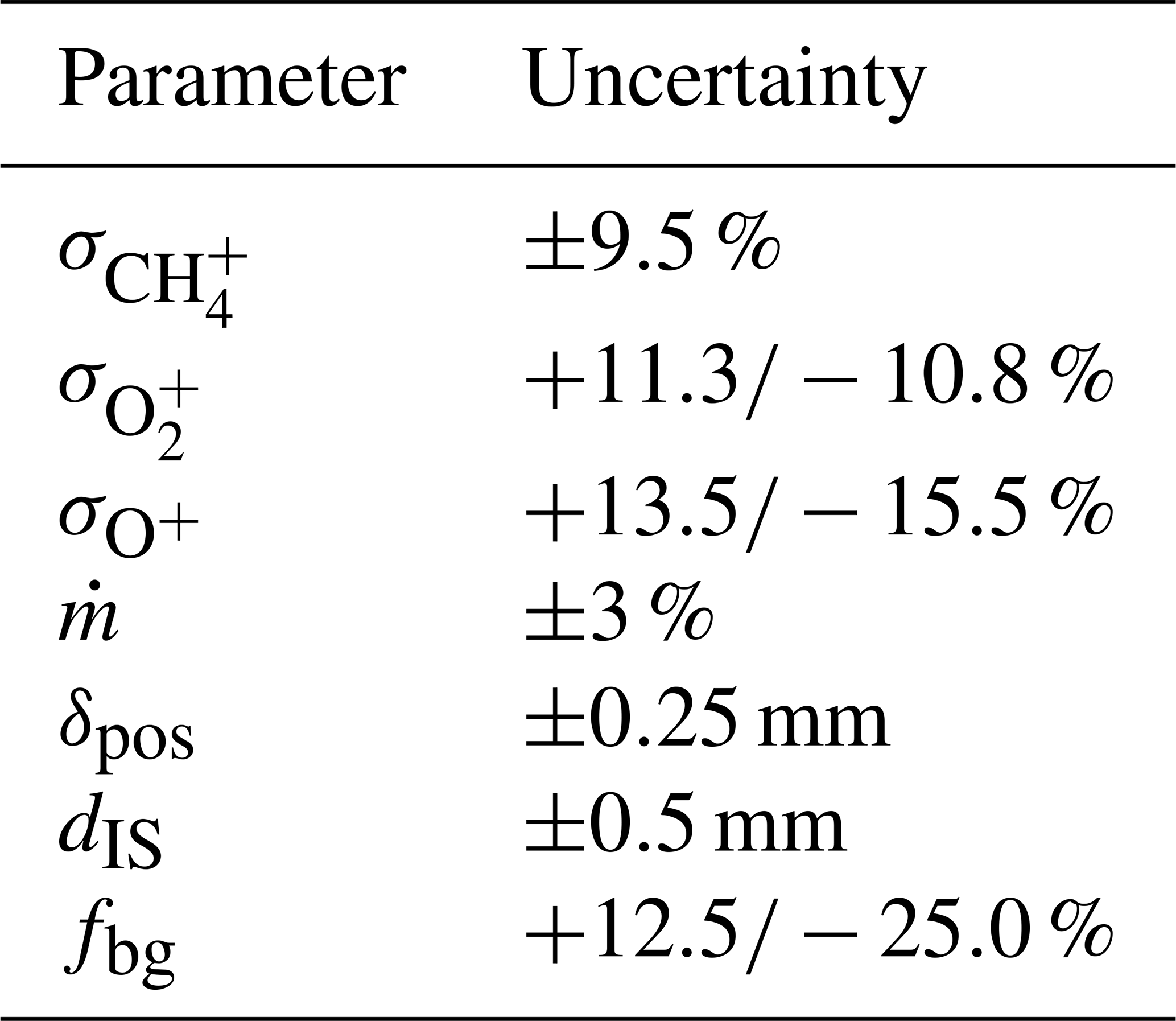
During the calibration, the local atomic oxygen number flux density at the sensor position is evaluated based on mass spectrometer data and the measured total mass flow rate within the molecular beam. The uncertainty of the result is therefore essentially composed of the uncertainties of the spectrometer, the flowmeter, the positioning of the sensors and additional geometrical quantities. All parameters that have been considered are summarized in Table A1 and are described in the following.

The employed mass spectrometer (Hiden HAL 3F) is a highly linear triple-filter instrument that was calibrated against a precise, gas-type-independent pressure sensor (MKS Baratron 690A) with an accuracy of reading of 0.12 % in the pressure range above $\mathrm{1}\cdot {\mathrm{10}}^{-\mathrm{5}}$ mbar (MKS, 2016). The main source of deviations here arises from the uncertainties of the ionization cross sections σ of the involved species. This includes uncertainties of the energy calibration of the ion source and of the literature values themselves. The combined uncertainties of the most relevant species (CH₄, O₂ and O) are given in the table.

The total mass flow rate $\dot{m}$ in the feed line and accordingly in the molecular beam was determined by a bubble flowmeter (Sigma-Aldrich). Despite its simple principle of operation, these instruments allow for the measurement of extremely small flows with an accuracy of up to 1 % (Levy, 1964). Based on numerous measurements, the uncertainty of the total mass flow rate in the current setup is estimated as 3 %. The radial profiles measured by the sensors and the mass spectrometer have to be taken at corresponding positions in the beam, and this matching can be done within the range δ_pos. The accuracy of the axial positioning of the spectrometer and its ion source is given as d_IQ. The measured radial profiles of the number densities within the molecular beam have to be mathematically separated from the background. As the linear travel of the spectrometer does not allow us to probe the real values outside of the beam, the background level has to be estimated from the border of the profile using the factor f_bg. Calibration curves for atomic oxygen as shown in Fig. 5 were then calculated under variation in these input parameters. For each measured sensor signal I_S the deviation of the number density n_O from its nominal value was determined, which corresponds to the single ΔR_i in Eq. (A1). The resulting total uncertainty maxima +35 % and −28 % are expressed as error bars in the calibration curve of sensor A23.

In principle, the sensor signal may be falsified by the presence of ozone, ions and excited molecular oxygen O₂(¹Δ_g). This source of error has to be considered for the calibration as well as during the rocket flight. Mass spectrometric methods proved that the molecular beam used in the calibration did not contain any of these problematic species (Eberhart et al., 2015). However, they may still exist in the atmosphere along the trajectory. Within the relevant altitude range the concentration of molecular oxygen in its excited state O₂(¹Δ_g) is below 0.5×10¹⁰ cm⁻³, 2 orders of magnitude lower than the maximum number density of atomic oxygen (Schiff, 1970). The literature does not give clear hints as to whether the sensor reaction could be affected by excited O₂ or not. In any case the effect is negligible within the MLT. In contrast to the stratosphere, the concentration of ozone is very low in the MLT (Allen et al., 1984) so that this source of uncertainty can be disregarded. Below the thermosphere, free charge carriers are very rare compared to atomic oxygen with number densities below 10⁵ cm⁻³ (Friedrich et al., 2012). These species, however, would follow an entirely different reaction mechanism on the sensor electrodes. Here further experimental work is required to estimate the uncertainty in the sensor signal.

Table A1 Parameters considered in the uncertainty analysis.

In addition to the experimental uncertainties discussed above the results from the aerodynamic simulation also have an influence on the density values. The uncertainty of the calculation is hard to quantify due to the lack of a true reference for the case of the payload aerodynamics. Instead, the reader is directed to the work by Bird that discussed the effects of aerodynamics on rocket-borne measurements (Bird, 1988).