the Creative Commons Attribution 4.0 License.
the Creative Commons Attribution 4.0 License.
 | 16 May 2019
Evolution of DARDAR-CLOUD ice cloud retrievals: new parameters and impacts on the retrieved microphysical properties
Quitterie Cazenave
Marie Ceccaldi
Julien Delanoë
Jacques Pelon
Silke Groß
Andrew Heymsfield
In this paper we present the latest refinements brought to the DARDAR-CLOUD product, which contains ice cloud microphysical properties retrieved from the cloud radar and lidar measurements from the A-Train mission. Based on a large dataset of in situ ice cloud measurements, the parameterizations used in the microphysical model of the algorithm – i.e. the normalized particle size distribution, the mass–size relationship, and the parameterization of the a priori value of the normalized number concentration as a function of temperature – were assessed and refined to better fit the measurements, keeping the same formalism as proposed in DARDAR basis papers. Additionally, in regions where lidar measurements are available, the lidar ratio retrieved for ice clouds is shown to be well constrained by the lidar–radar synergy. Using this information, the parameterization of the lidar ratio was also refined, and the new retrieval equals on average 35±10 sr in the temperature range between −60 and −20 ∘C. The impact of those changes on the retrieved ice cloud properties is presented in terms of ice water content (IWC) and effective radius. Overall, IWC values from the new DARDAR-CLOUD product are on average 16 % smaller than the previous version, leading to a 24 % reduction in the ice water path. In parallel, the retrieved effective radii increase by 5 % to 40 %, depending on temperature and the availability of the instruments, with an average difference of +15 %. Modifications of the microphysical model strongly affect the ice water content retrievals with differences that were found to range from −50 % to +40 %, depending on temperature and the availability of the instruments. The largest differences are found for the warmest temperatures (between −20 and 0 ∘C) in regions where the cloud microphysical processes are more complex and where the retrieval is almost exclusively based on radar-only measurements. The new lidar ratio values lead to a reduction of IWC at cold temperatures, the difference between the two versions increasing from around 0 % at −30 ∘C to 70 % below −80 ∘C, whereas effective radii are not impacted.
- Article
(7774 KB) - Full-text XML
- BibTeX
- EndNote


Passive and active remote sensing instruments, like visible and infrared (IR) radiometers, cloud radars, and lidars, are commonly used to study ice clouds. Inferring cloud microphysical properties like extinction (α), ice water content (IWC), and effective radius (re) can be done from one instrument only or from the synergy of several instruments or channels (i.e. wavelengths λ). Several methods were developed to retrieve ice cloud properties from a single instrument: IR radiometers are commonly used to retrieve integrated re from a set of brightness temperatures at different wavelengths (Stubenrauch et al., 1999; Guignard et al., 2012; Hong et al., 2012), and lidars and radars are useful to retrieve respectively extinction and IWC (Liu and Illingworth, 2000; Vaughan et al., 2004; Heymsfield et al., 2014). However, all of these instruments have shortcomings in different parts of the cloud – for instance, due to the attenuation of the lidar signal, the lidar will be blind in the lower part of a thick cirrus, whereas the top of the cloud is invisible to the radar in most cases – resulting in a large spread of values for the retrieved cloud properties. Hence, there is a need to use several instruments to reduce this uncertainty. Synergetic ice property retrieval methods can combine radiometer with lidar or radar (Evans et al., 2005; Garnier et al., 2012, 2013; Sourdeval et al., 2014) or both lidar and radar (Donovan et al., 2001; Wang and Sassen, 2002; Okamoto et al., 2003; Delanoë and Hogan, 2008, 2010, hereafter referred to as DH0810).
Radar and lidar are active sensors that provide vertical information on cloud structure and are sensitive to different cloud particle populations. To a first approximation, the radar return signal is proportional to the sixth moment of the particle size; hence, within a volume it is most sensitive to the largest particles. On the other hand, lidar backscatter is proportional to the second moment of the particle size and is thus more sensitive to particle concentration and backscattering cross section. Combining the two instruments therefore provides two moments of the particle size distribution. In regions of the cloud where both instruments are available, this method allows a well-constrained retrieval of extinction and IWC, leading to direct calculation of re at each pixel of the vertical profile obtained by this synergy. The difference in sensitivity of the two instruments also gives a more complete view of the cloud structure and microphysics (Donovan et al., 2001; Okamoto et al., 2003; Tinel et al., 2005).
The A-Train constellation of satellites has considerably improved our knowledge of clouds. Since 2006, CALIPSO (Cloud-Aerosol Lidar and Infrared Pathfinder Satellite Observation) and CloudSat have acquired cloud vertical profiles globally. CALIPSO (Winker et al., 2010) carries CALIOP (Cloud-Aerosol Lidar with Orthogonal Polarization), a lidar operating at 532 and 1064 nm with depolarization capabilities on the 532 nm channel (Winker et al., 2007), as well as the Imaging Infrared Radiometer (IIR) and a Wide Field Camera (WFC). CloudSat carries a Cloud Profiling Radar (CPR) measuring reflectivity at 95 GHz (Stephens et al., 2002). Lidar–radar synergetic methods have been adapted to CloudSat and CALIPSO data (Okamoto et al., 2010; Delanoë and Hogan, 2010; Deng et al., 2010). In this paper, we focus on the DARDAR-derived products. The DARDAR (raDAR/liDAR) project was initiated by the LATMOS (Laboratoire Atmosphères, Milieux, Observations Spatiales) and the University of Reading. It was developed to retrieve ice cloud properties globally from CloudSat and CALIPSO measurements using a specific universal parameterization of the particle size distribution (Delanoë et al., 2005, 2014) and the Varcloud optimal estimation algorithm (DH0810). DARDAR has three products that can be used separately, and they are all hosted and available on the ICARE (Interactions Clouds Aerosols Radiations Etc) FTP website at ftp://ftp.icare.univ-lille1.fr/ (last access: 9 May 2019). The first one is the CS-TRACK product, which is the collocated processed A-Train product on the CloudSat track. This product gives the possibility to work on lidar and radar data on the same resolution grid of 1.1 km horizontally and 60 m vertically. From these profiles of active instruments data, a technique for the classification of hydrometeors (called DARDAR-MASK) has been developed. This technique is used to select the lidar–radar range bins (or pixels) where ice cloud property retrievals (DARDAR-CLOUD) can be performed (Ceccaldi et al., 2013). It is important that the classification is as accurate as possible since including liquid water pixels or noisy pixels in our retrieval could compromise the results. Indeed retrieval techniques are different for liquid droplets and for ice crystals, and a specific analysis should be applied to mixed-phase clouds (Hogan et al., 2003). In this paper, we only focus on the retrieval of ice crystal properties.
From collocated profiles of CloudSat and CALIPSO and hydrometeor classification, the DARDAR-CLOUD algorithm performs retrievals of extinction, IWC, and re at each pixel of ice cloud detection (even when only one instrument is available) on the CS-TRACK grid. The main advantage of DARDAR, compared to many other synergetic methods, is that it seamlessly performs retrievals in cloud regions detected by both the radar and the lidar and in regions detected by only one instrument. This is achieved using an optimal estimation algorithm, finding the best state vector of cloud properties which minimizes the errors on observations (radar reflectivity Z and lidar apparent backscatter βa) compared to measurements simulated using a forward model. Whenever one of the measurements is missing, the algorithm relies on an a priori estimate of the state vector derived from the climatology.
The DARDAR-CLOUD product has been widely evaluated and used (Deng et al., 2013; Delanoë et al., 2013; Hong and Liu, 2015; Sourdeval et al., 2016; Saito et al., 2017), and a few issues have been identified. For example, Deng et al. (2013) compared DARDAR-CLOUD with other satellite products and with cloud properties derived from aircraft in situ measurements obtained with a 2D-S probe, during the SPARTICUS campaign in 2010. Compared to the other CloudSat-CALIPSO product and the aircraft observations, the DARDAR-CLOUD product seemed to overestimate IWC in cloud regions where only lidar measurements were available. Sourdeval et al. (2016) also compared the ice water path (IWP) retrieved with different satellite products over the year 2008 and highlighted the fact that the DARDAR-CLOUD product tends to overestimate IWP, in particular for values below 10 g m−2. As a consequence, adjustments have been made to the algorithm to optimize retrievals as a function of range and temperature, especially concerning the detection of ice particles and the cloud microphysical model, keeping the formalism unchanged from DH0810. In the following, the new version of DARDAR-CLOUD resulting from those changes will be called V3, and the version available on the ICARE website until 2018, namely DARDAR-CLOUD v2.1.1, will be referred to as V2. It is important, for the consistency of future studies compared to earlier ones, to give information on the differences between the two versions and the way they impact the results of the algorithm. After introducing the key features of the variational scheme in Sect. 2, its recent updates are detailed in Sect. 3, and their effects on the retrieved cloud microphysical properties are presented in Sect. 4. We will mainly focus on the retrieval of IWC and briefly present the main differences observed on the retrieved particle sizes.
We summarize here the main characteristics of the inverse method used for the DARDAR retrievals; readers interested in details of the Varcloud algorithm are invited to check on DH0810.
The method is applied to one profile at a time. We start with a first guess of the state vector on the pixels of the profile where the retrieval can be performed (i.e. ice-only pixels). A forward model is applied to this state vector to compute simulated values of the radar reflectivity (Zfwd) and the lidar attenuated backscatter (βfwd) of those ice pixels. The state vector is updated until convergence is achieved (when Zfwd and βfwd are close enough to Z and βa observations, or when iterations do not produce better results). A priori information about this state vector – derived from a climatology of airborne, ground-based, and previous satellite measurements – is used to constrain the inverse problem. This is useful when only one measurement is available. Indeed, in most cases, when a cloud profile is measured by both radar and lidar, the vertical fraction of the cloud detected by both instruments is often preceded in the upper layers by a region only detected by the lidar and followed by a region detected by the radar alone in the lower part. In such regions, the algorithm needs additional information to ensure that the state vector tends towards a physical value.
The state vector contains the cloud properties that we want to retrieve. In the case of Varcloud, it is composed of visible extinction (αv) (), lidar extinction-to-backscatter ratio (S) (sr), and which can be considered a proxy for the particle number concentration. Contrary to αv, S and are not defined at every valid pixel of the cloud profile. The definition of the profile within the state vector is given by DH0810; we will therefore not go into further details. The lidar ratio (inverse of the value of the normalized phase function at 180∘) is a function of many microphysical parameters such as the particle size and shape as well as its orientation (Liou and Yang, 2016). Those variables are expected to vary through the cloud profile. The total attenuated backscatter signal alone, measured by CALIOP, is not enough to give information on this height dependence. However, to account for the variation of S along the cloud profile, the final expression that was set for DARDAR-CLOUD V2 is based on a parameterization with the temperature. Following Platt et al. (2002), ln(S) is assumed to vary linearly with temperature (in ∘C):
This parameterization allows the coefficients alnS and blnS to be used to represent S in the state vector and simplify the iteration process.
Table 1Coefficients used in the parameterization of the a priori value of S.
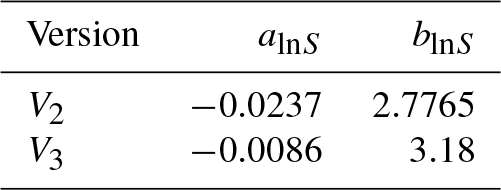
Table 2Coefficients used in the parameterization of the a priori value of .
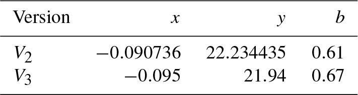
A priori information is only necessary for S and since the extinction is already well constrained by both the radar and the lidar. Regarding the lidar ratio, an a priori value is determined for each of the two coefficients alnS and blnS (see Table 1). Following DH0810, the a priori value of is also expressed as a linear function of temperature:
with T in degrees Celsius (∘C). Physically, this describes the idea that as the temperature gets warmer, the aggregation processes tend to increase the size of the particles and reduce their number (x<0). Values of x and y are given in Table 2.
Errors ascribed to the a priori represent how strong this constraint is: the larger the error on the a priori value, relative to the measurement error, the less relevant the difference between the actual value of the state vector and the a priori is and the more the state vector will be allowed to move away from it. The straightforward way to account for the uncertainty on the a priori information is to use an error covariance matrix with constant diagonal terms, assuming the confidence we have in this information is the same everywhere in the cloud profile. When both instruments are available, hopefully the confidence in the measurements is higher than in the a priori value, and the algorithm does not rely on this information. Conversely, in regions where only one instrument is available, the retrieved values of S and would essentially be determined by the a priori value. Therefore, to allow the information from synergistic regions to propagate towards regions where fewer measurements are available, additional off-diagonal elements are added to the error covariance matrix of the a priori value. Those off-diagonal terms decrease exponentially as a function of the distance and aim at describing a spatial correlation in the difference between the actual value of and its a priori value. This spatial correlation in the retrieval of is of course transmitted to the other cloud variables through optimal estimation. More details can be found in Delanoë and Hogan (2008).
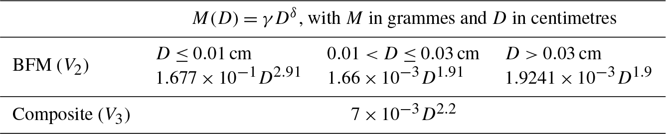
Finally, a microphysical model is needed. First of all, an equivalent diameter for ice crystals Deq has to be used. It corresponds to the diameter the particle would have if it were a spherical liquid droplet of the same mass M. It can be expressed as follows:
with ρw=1000 kg m−3 the density of water. To be able to determine Deq for any ice crystal, we introduce a relationship giving the mass of a particle as a function of its maximum diameter. This relationship is usually described as a power law of diameter: M(D)=γDδ (Brown and Francis, 1995; Mitchell, 1996; Lawson and Baker, 2006; Heymsfield et al., 2010; Erfani and Mitchell, 2016). For DARDAR-CLOUD V2, a combination of Brown and Francis (1995) and Mitchell (1996) for hexagonal columns is used. This relationship will be referred to as “BFM” in the rest of the paper. Its expression can be found in Table 3.
A particle size distribution (PSD), describing the concentration of particles as a function of diameter, N(D), is then defined as a function of Deq. To do so, following Delanoë et al. (2005), both diameter and concentration are scaled so that it is possible to find a functional form F fitting any measured PSD appropriately normalized:
The equivalent diameter is scaled by the mean volume weighted diameter, Dm, defined as the ratio of the fourth to the third moments of the PSD, in terms of Deq:
and the number concentration is scaled by (m−4), which can be written as follows:
is also linked to via the relationship , with b a coefficient determined from in situ microphysical measurements. The b values used for V2 and V3 can be found in Table 2.
Table 4Parameters of the modified gamma shape used to approximate the normalized PSD.
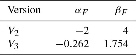
The function in Eq. (4) can be approximated by a two-parameter modified gamma shape , the two parameters being determined by a statistic of in situ measurements (see Delanoë et al., 2014, for the detailed expression of F and Table 4 for the values of αF and βF). With this normalized particle size distribution and for a given range of Dm, it is then possible to create a 1-D lookup table (LUT) linking all the cloud microphysical variables to the ratio of αv to . This LUT is used in the forward model within the iterative process, in particular to retrieve from . The reflectivity is defined following Eq. (7):
with the scattering cross section σ(D) obtained by the T-matrix method and Mishchenko et al. (2004) spheroid approximation for randomly oriented particles. Once the optimized cloud profile has been determined, this same LUT is also needed to retrieve additional features of the profile, such as the IWC and effective radius.
The general method described above has remained unchanged since the creation of the DARDAR-CLOUD V2 products. In this paper, we only show improvements that were made in the parameterizations of the microphysical model and the a priori relationships.
This article presents the upgrade of the DARDAR-CLOUD product after the DARDAR-MASK product was modified (Ceccaldi et al., 2013). In this section we describe the improvements on the lidar ratio a priori and the microphysical model used in the retrieval method, before quantifying their impacts in the next section.
3.1 A priori information for the lidar ratio
In DARDAR-CLOUD V2 the a priori relationship linking S to the temperature was , with T in degrees Celsius (∘C). This was found to produce values of S that are too large at cold temperatures (up to 120 sr) compared to the climatology. Indeed, several studies on semi-transparent cirrus clouds were performed with elastic lidars in the visible, either from airborne (Yorks et al., 2011), ground-based (Platt et al., 1987, 2002; Chen et al., 2002), or space-borne (Garnier et al., 2015) instruments. In all cases, retrieved lidar ratios were found around an average value of 25–30 sr and rarely exceeded 50 sr. In addition, more studies were done on cloud optical properties, including measurements performed in the UV by Raman ground-based lidars, showing similar values for the retrieved lidar ratios (Whiteman et al., 2004; Thorsen and Fu, 2015). In order to rectify this problem and produce more sensible retrievals, a new a priori relationship was determined for S. To do so, a linear regression is performed on the distribution of the retrieved lnS as a function of temperature, using only lidar–radar synergistic areas. In such regions, the retrieval of S is expected to be well constrained by the measurements. To be even less dependent on the a priori value, the old parameterization is kept but with an error on the slope coefficient (alnS) multiplied by 10. To produce the statistic of lidar ratio used in this study, the Varcloud algorithm was run on 10 d of CloudSat-CALIPSO observations of the year 2008. The results of the regression are presented in Fig. 1. The regression was performed on the logarithm of S. The large majority of points are located in regions where the temperature ranges from −55 to −20 ∘C, which are the temperatures for which synergistic measurements are statistically most likely to be found. In this domain of temperatures, one can see that the mean and median values of lidar ratio for the different temperature bins are almost identical and fairly close to the first mode of the distributions, which allows for a good assessment of the lidar ratio, as shown by the result of the linear fit. Conversely, except for the warmest temperatures (above −30 ∘C), the old parameterization clearly overestimates the lidar ratio. For colder and warmer temperatures (below −55 and above −20 ∘C, respectively) the slope of the mean curve changes, with the lidar ratio shifting to values <30 sr. This leads to a rather low correlation coefficient (−0.3) for the linear regression. Indeed, the fitting process is mainly constrained by the central region where most of the data are found and therefore cannot account for the different behaviour of the lidar ratio at the edges of the temperature domain. This illustrates the fact that the variation of the lidar ratio along the cloud profile cannot only be described by the temperature. The comparison of this study to the one from Garnier et al. (2015) confirms this: they are in good agreement where the temperature domains overlap. But as only cold semi-transparent cirrus measured by the lidar and the radiometer are represented in Garnier et al. (2015), the behaviour is different, and the lidar ratios retrieved at temperatures below −60 ∘C are lower (up to 50 % lower at −70 ∘C).
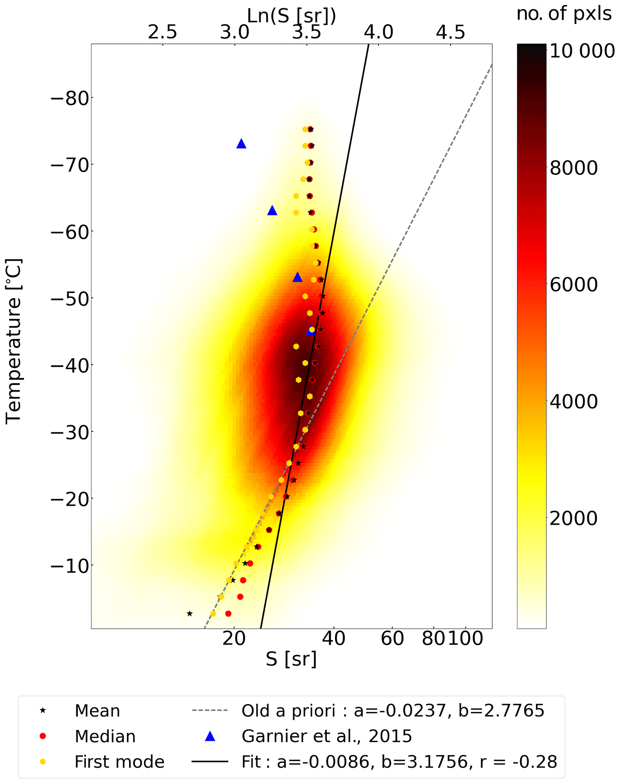
Figure 1Linear regression on the probability density distribution of ln(S) as a function of temperature. The corresponding values of S in steradian (sr) are also displayed. The result of the linear regression fit is represented by solid lines and the old a priori relationship by dashed lines. Red and yellow dots are the median and first mode (respectively). The parameterization obtained with the retrievals from Garnier et al. (2015) is also displayed for comparison (blue triangles).
Additionally, multiple scattering is not accounted for the same way. Based on the work by Platt (1973), Garnier et al. (2015) define a multiple scattering factor to correct the two-way transmittance from the contribution of multiple scattering. This correction factor equals 1 in the single-scattering limit and varies from 0.5 to 0.8 as a function of temperature for the CALIOP instrument. In the Varcloud algorithm, multiple scattering is accounted for in the lidar backscatter forward model that was developed by Hogan (2008). This forward model uses a fast, approximate analytical method based on the representation of the photon distributions by their variance and covariance to infer multiple scattering effect at each gate of the measured profile.
However, this approximation appears to be legitimate in the lidar–radar areas and is considered valid as a priori information on the entire profile, even though larger errors can be expected in lidar-only regions. The final coefficients are chosen to be and blnS=3.18, as reported in Table 1. Reducing the slope coefficient should prevent the occurrence of values for S that are too high at the coldest temperatures.
3.2 The microphysical model
The microphysical model is based on three main parameterizations: the normalized PSD, the a priori of , and the mass–diameter relationship.
For DARDAR-CLOUD V2, the parameterizations of the PSD and the a priori of were determined using the in situ dataset described by Delanoë et al. (2005). The main caveat of this study is that it did not use direct measurements of IWC, which may question the reliability of the validation of the microphysical model. The idea here is to assess and refine these parameterizations, using a more comprehensive and accurate dataset of ice cloud in situ measurements.
Delanoë et al. (2014) present a large in situ dataset collected during several ground-based and airborne campaigns between 2000 and 2007. During those campaigns, direct measurements of IWC were performed with a Counterflow Virtual Impactor or a Cloud Spectrometer and Impactor (CVI/CSI). Such instruments provide valid measurements in the range from 0.01 to 2 g m−3. For a better quality control of the measured PSD, the shattering effect was also considered in this study.
Using the same in situ dataset, a series of M(D) relationships have been derived by Heymsfield et al. (2010) for specific cloud conditions. Delanoë et al. (2014) compared the measured bulk IWC to the retrieved IWC obtained by the combination of the measured PSD and one of those power laws, which allowed the M(D) relationship giving the best match to the measured IWC to be selected for each campaign. A description of the selected M(D) is given in Delanoë et al. (2014) (Table 3). The general mass–size parameterization, specific to this dataset and made of different power laws as a function of the measurement campaign, will be referred to as the “RETRIEVED” parameterization.
The BFM mass–size relationship used in DARDAR-CLOUD V2 was validated on direct measurements of IWC, using a total water content probe combined with a fluorescence water vapour sensor. However, those measurements were restricted to a couple of flights performed in April 1992 over the North Sea and to the south-west of the UK, providing a dataset of fewer than 3000 points recorded at temperatures between −30 and −20 ∘C. Other relationships are described in the literature, for specific types of clouds, crystal habits, or temperature ranges (see Heymsfield et al., 2010, and Erfani and Mitchell, 2016). To account for the dependency of the relationship between D and M on temperature and particle size, Erfani and Mitchell (2016) propose to use a δ coefficient depending on temperature. However, temperature is not the only parameter that matters for the determination of M(D). In order to accurately fit this relationship to each and every cloud situation, we would need more information on cloud type and particle size, which are not straightforward to derive from the CloudSat-CALIPSO synergy. In addition, it is difficult to change M(D) in the retrieval scheme upon the cloud type and the meteorological conditions without risking bringing discontinuity into the retrievals. As a result, in the case of the DARDAR-CLOUD product, we decided to focus on statistical results and assume a single M(D) relationship which can work for most of the situations.
In the following, we detail how the dataset presented by Delanoë et al. (2014) was used to refine the microphysical model of the Varcloud algorithm.
3.2.1 The normalized PSD
The normalized particle size distribution is updated with the new coefficients determined by Delanoë et al. (2014) using a least squares regression on two moments of the PSD, namely the visible extinction, αv, and the radar reflectivity, Z. To do so, a mass–size relationship had to be assumed, and the RETRIEVED parameterization was chosen. Figure 2 compares the shape of the normalized PSD for the two versions of DARDAR-CLOUD, V2 and V3. The different coefficients are reported in Table 4. The new coefficients mainly impact the very small diameters and the tail of the distribution. The centre of the distribution (around ) remains almost unchanged. However, the new normalized PSD is now characterized by higher values of normalized number concentration for the largest particles. This could increase the impact of the change in the mass–diameter relationship. Additionally, it is reminded here that in a first-order approximation, the radar reflectivity is more sensitive to the size of the particles, whereas the lidar backscatter depends mainly on the concentration. As a result, if the weight on the large particles is increased, a higher sensitivity can be expected in regions detected by the radar. However, as presented by Delanoë et al. (2014), the majority of the data are concentrated in the area where . The change in M(D) is therefore expected to be of more importance than the modification of the normalized particle size distribution.

Figure 2Lookup table parameters: the normalized PSD (DARDAR-CLOUD V2 is represented by the black dashed line, and the new parameterization, V3, is represented by the red solid line).
3.2.2 The a priori value of
As mentioned previously, the a priori value for is obtained via a parameterization as a function of the temperature. Three parameters have to be determined. The first two are used to link to the temperature, and the last one, b, relates to the normalized number concentration . To do so, several linear regressions are performed between and T to identify the x and y parameters for different values of b. The values of and αv are retrieved from the measured PSDs and the RETRIEVED M(D) laws. The final set of parameters is chosen with the highest coefficient of determination R2. For this study, the “subvisible” class in the dataset presented in Delanoë et al. (2014) has been removed as it consists of very small crystals associated with very cold temperatures, and we considered that it was too far from the main common radar–lidar domain in terms of temperature conditions. The data points measured at temperatures above −15 ∘C during the MPACE campaign have also been removed.
Figure 3 shows the result of the regression, and the coefficients are reported in Table 2. The new a priori parameterization for as a function of T is very close to the old version (Fig. 3b). The main difference is for the b coefficient, which leads to an increase in the corresponding value of of almost 2 orders of magnitude.

Figure 3Determination of the a priori value of : values of the coefficient of determination R2 for different values of b and values of the coefficients for the best fit (a), result of the linear regression on for the entire dataset as a function of temperature (with b=0.67) (b) and corresponding for different values of extinction (c).
3.2.3 The mass–diameter relationship
Figure 4 shows the comparison between the measured IWC and the retrieved IWC, for different mass–diameter relationships: the RETRIEVED parameterization, for which a specific power law is selected for each campaign (panel a), the parameterization used in DARDAR-CLOUD V2, namely BFM, applied to all the campaigns (panel b), and finally the “Composite” parameterization, also applied to the entire dataset (panel c). The Composite was developed by Heymsfield et al. (2010) using the measurements of all campaigns, combining different types of clouds and situations. As we want to keep a single M(D) in our algorithm, it is interesting to compare this more recent parameterization to BFM.
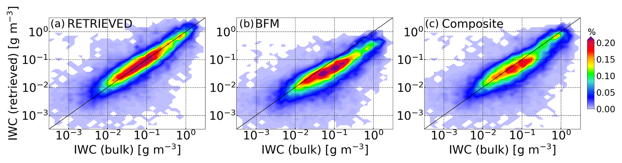
Figure 4Comparison between the measured IWC (horizontal axis) and the retrieved IWC using different mass–diameter relationships (vertical axis): RETRIEVED (Delanoë et al., 2014) (a), BFM (Brown and Francis, 1995; Mitchell, 1996) (b), and Composite (Heymsfield et al., 2010) (c).
It is clear that using dedicated parameterizations for specific atmospheric conditions and/or cloud types (that is, the RETRIEVED parameterization) gives better results when comparing the model to the measurements. However, in the framework of our retrieval scheme, we prefer to use one parameterization which gives the best fit, on average. Hence the choice of BFM for DARDAR-CLOUD V2. As presented in Fig. 4b, this parameterization critically underestimates the measured IWC, especially for values above 0.1 g m−3. With the Composite relationship, on the contrary, it is possible to improve the match with the measured IWC (panel c). It was therefore decided to modify Varcloud's microphysical model and use Composite instead of BFM. Details of these two relationships can be found in Table 3. The main difference between the expressions of BFM and Composite is the power coefficient: for particles >100 µm, this coefficient equals 1.9 for BFM, and it equals 2.2 for Composite. As a result, for a given mass, the Composite relationship provides a smaller equivalent diameter for the ice crystal than BFM. This difference increases when the mass and the size get larger. On the contrary, for small diameters (≤100 µm), BFM creates denser particles with smaller Deq. Referring to Erfani and Mitchell (2016), these δ coefficients are in the domain of optimal values for ice crystals from continental ice clouds, at temperatures between −60 and −20 ∘C and of size ranging from 100 to 1000 µm. Moreover, they showed that the Composite M(D) conformed closely to their fit performed on measurements from the SPARTICUS campaign.
DARDAR-CLOUD V2 was created using the DARDAR-MASK v1 classification to select the hydrometeors on which to perform the retrieval. Since the classification was updated by Ceccaldi et al. (2013) (DARDAR-MASK v2), we will briefly show in a first instance the impact of the change in classification on the microphysical properties. In a second instance, we will present how the modifications of the a priori value and the microphysical model presented in the previous section impact the retrieval of the lidar ratio, IWC, and effective radius.
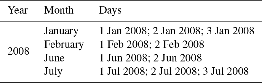
The analysis is done over the same 10 d (∼3M profiles) of CloudSat-CALIPSO observations as those used to determine the new a priori value for the lidar ratio. The details of this dataset are presented in Table 5. All the studies presented in this paper were performed using the same set of observations.
4.1 Impact of the new classification
As detailed in Ceccaldi et al. (2013) the new hydrometeor classification (DARDAR-MASK v2) reports fewer ice clouds in the upper troposphere than DARDAR-MASK v1. This is due to the fact that the new methodology is more restrictive in creating the lidar mask in order to include as few noisy pixels as possible. On the other hand, it can miss some very thin ice clouds. Also, the false cloud tops detected by the radar due to its original resolution have been removed from the radar mask; hence fewer fake ice pixels are retrieved on radar-only data on top of lidar–radar pixels.
To study the impact of the new classification on the retrieved IWC we run the algorithm with the DARDAR-CLOUD V2 configuration with both the old and the new classifications. The distribution of derived log10(IWC) as a function of temperature is then compared.
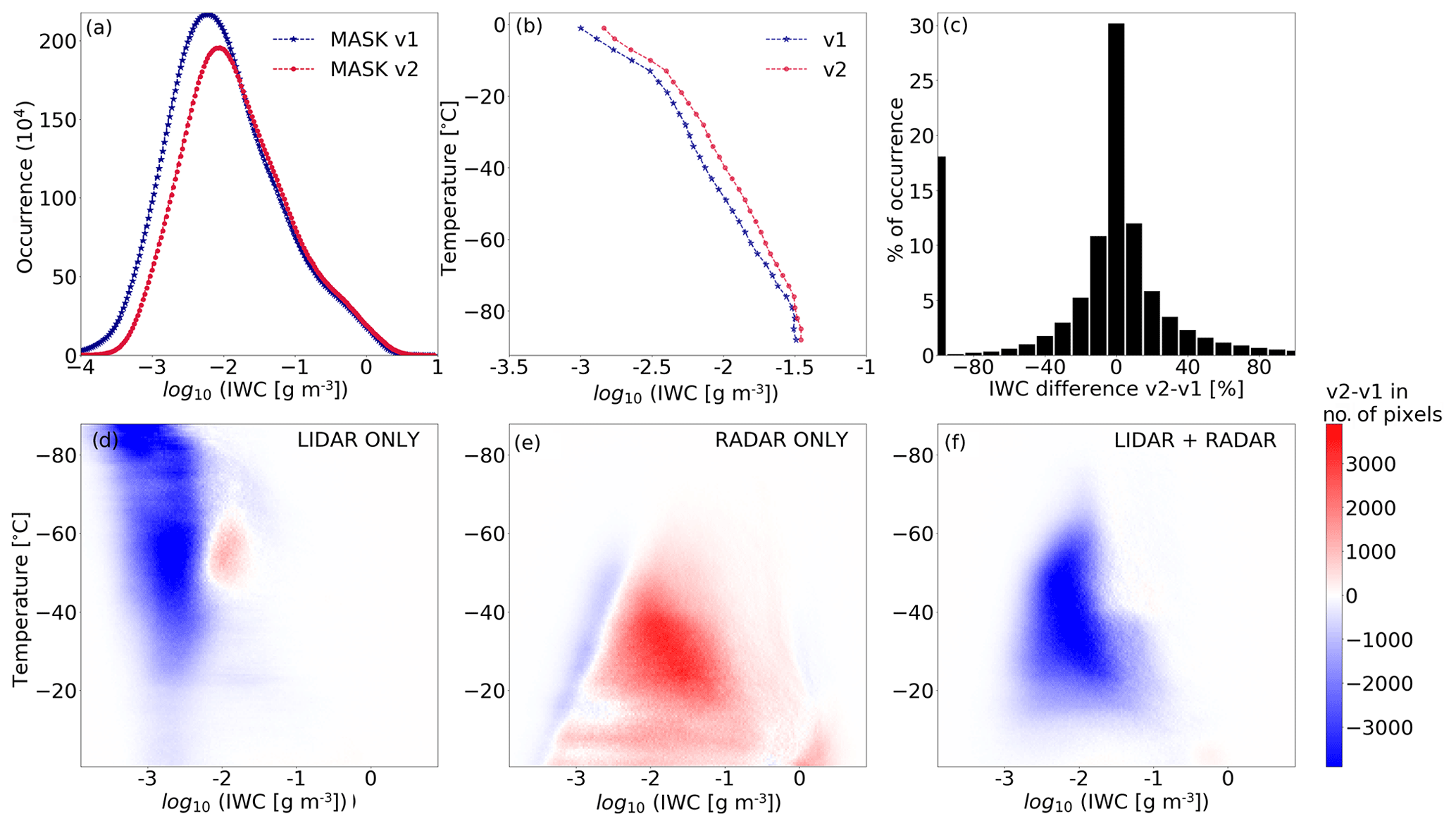
Figure 5Comparison of DARDAR-MASK v1 and DARDAR-MASK v2 in terms of IWC retrieved using Varcloud (V2): histograms of log10(IWC) (a) with the old version of DARDAR-MASK in dashed line and the new version in solid line, the mean of the distribution of log10(IWC) as a function of temperature (b) for DARDAR-MASK v1.1.4 (dashed line) and DARDAR-MASK v2.1 (solid line), the histogram of the relative difference between DARDAR-MASK v2 and DARDAR-MASK v1 (c), and the difference between the two configurations in terms of number of pixels in each [T−log10(IWC)] bin for lidar-only pixels (d), radar-only pixels (e), and pixels combining the two instruments (f).
The distributions are computed as the histogram of occurrence (as percentage of pixels included in the retrieval) of log10(IWC) in temperature bins of 0.5 ∘C in the range −88 to 0 ∘C. The comparison between the two distributions is displayed in Fig. 5. We can see that using the new classification globally leads to fewer pixels included in the retrieval, especially for IWC lower than 10−2 g m−3 (Fig. 5a). Consequently the mean log10(IWC) decreases more rapidly with decreasing temperature than when using the old classification (Fig. 5b). This observation is consistent with the fact that the new classification is more restrictive; lidar noisy pixels and very thin ice clouds pixels producing very low IWC are not included in this distribution any longer, leading to higher mean values. This is highlighted by the comparison of both distributions in the lidar-only region (Fig. 5d). It is very clear that fewer pixels are selected in the new version, especially for g m−3. There are also fewer pixels of low IWC in the radar-only regions (panel e) due to the suppression of fake cloud top detection on the radar signal.
This new selection of cloud pixels on the lidar signal also affects the synergistic areas. Indeed, if fewer lidar pixels are detected, then the number of lidar–radar pixels decreases in favour of radar-only pixels. In such regions, most of the pixels that were removed from the lidar cloud mask are suspected to be noisy measurements. Including noise in a variational retrieval can increase its instability and lead to higher errors. It is therefore safer to have fewer but more reliable pixels in common for the two instruments. On the other side, the number of higher IWC values ( g m−3) is slightly enhanced. The way the new categorization better deals with the radar's ground clutter could account for more radar and lidar–radar areas detected as ice clouds close to the ground, with temperatures between −10 and 0 ∘C.
When comparing the two configurations pixel by pixel, one can see that no bias is introduced by the new classification as the histogram of differences is centred on 0 %. As a consequence, the increase in the mean of retrieved IWC is solely due to the removal of pixels of very low IWC values. The 18 % of the data showing −100 % difference account for pixels that used to be classified as ice in the old configuration and that are not detected by the new algorithm because they are suspected of being noisy pixels. Pixels that are not affected by the new classification show on average the same values of IWC. Overall, more than 50 % of the data show less than 20 % difference. Larger differences appear in profiles where ice pixels were removed or added, which potentially changed the balance between the instruments.
For the following studies, the algorithm is applied to the new classification, and both instruments are used whenever available.
4.2 Impact of the new a priori relationship for the lidar ratio
To be more consistent with the extinction-to-backscatter ratio (S) values found in the literature and to account for the assessment done on the retrieved IWC in high troposphere (Deng et al., 2013), a new a priori value was determined using the well-constrained retrievals from the radar–lidar synergistic areas (Sect. 3.1). To assess the impact of this new configuration on the retrievals, the Varcloud algorithm was run using the two different a priori relationships for S one after the other.
4.2.1 S retrievals
With the new parameterization, one can see that the values are, on average, smaller and more centred around an average value of 35 sr (Fig. 6a). As a result, contrary to what could be found with the old configuration, the maximum values do not exceed 60 sr. Panels (b) to (j) show the distributions (in % of the total number of retrieved pixels) of S for the two different configurations as well as the distributions of their relative difference as a function of temperature. As a consequence of this new configuration, the retrieved lidar ratio tends to be closer to the a priori value. This new parameterization was determined using former Varcloud retrievals; therefore it is logical that the fit to the algorithm is better. This is particularly visible when comparing panels (c) and (f) for lidar-only areas.

Figure 6Comparison of the retrieved lidar ratios for two a priori parameterizations: histograms of S (a) with the old a priori relationship (dashed) and the new relationship (solid), probability density distributions of S as a function of temperature obtained when using the old configuration (b–d) and the same results with the new configuration (e–g), probability density distribution of the relative difference between the two lidar ratios obtained from the two different configurations at each retrieved pixel (h–j). The black line represents the a priori value.
As the algorithm only returns the two coefficients of the relation linking lnS to T, the retrieved lidar ratio depends on the measured profile as a whole. For stability reasons, the error applied to the a priori value is small. As a result, the lidar ratio mainly follows the a priori information. But it is allowed to move away from it, especially in synergistic areas where more information is provided to the state vector by the radar. This explains the two modes observed on the relative difference distributions. One mode is closer to 0 % difference (between −25 and +25 %) and corresponds to profiles where the retrieval of the lidar ratio can benefit from the synergy of radar and lidar. It is therefore less constrained by the a priori information, and the new parameterization has less impact in these regions. The second mode follows a thin line representing the difference between the two a priori slopes. This mode contains profiles for which the a priori value has the major influence in determining the lidar ratio, e.g. profiles with lidar measurements alone. The uncertainty in the retrieval of the lidar ratio as well as the influence of the a priori information in these regions could be further reduced using additional sensors such as IR or/and visible radiometers.
4.2.2 IWC retrievals
These differences in lidar ratio can impact the ice water content via the visible extinction. Differences in log10(IWC) distribution are shown in Fig. 7. As expected, changing the configuration only impacts IWC below 10−1 g m−3. Indeed, we expect IWC above this threshold to be found in the lower parts of the clouds, where only the radar can provide measurements, and therefore the impact of the lidar ratio a priori can be neglected. The global distribution of log10(IWC) is shifted towards lower values, and the lower the IWC, the more differences can be seen.
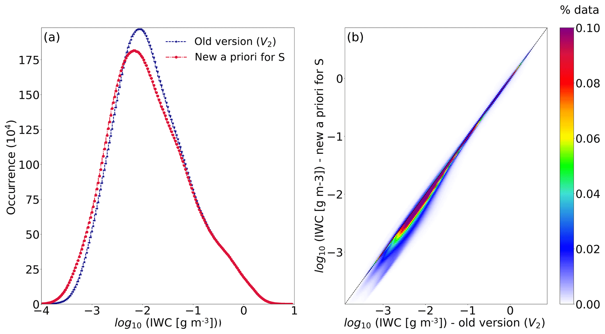
Figure 7Comparison of the retrieved IWC for two a priori parameterizations of the lidar ratio: panel (a) shows the histograms of log10(IWC) using the old (V2) a priori relationship (dashed) and the new (V3) relationship (solid). Panel (b) shows the probability density distribution of each IWC retrieval relative to the other.
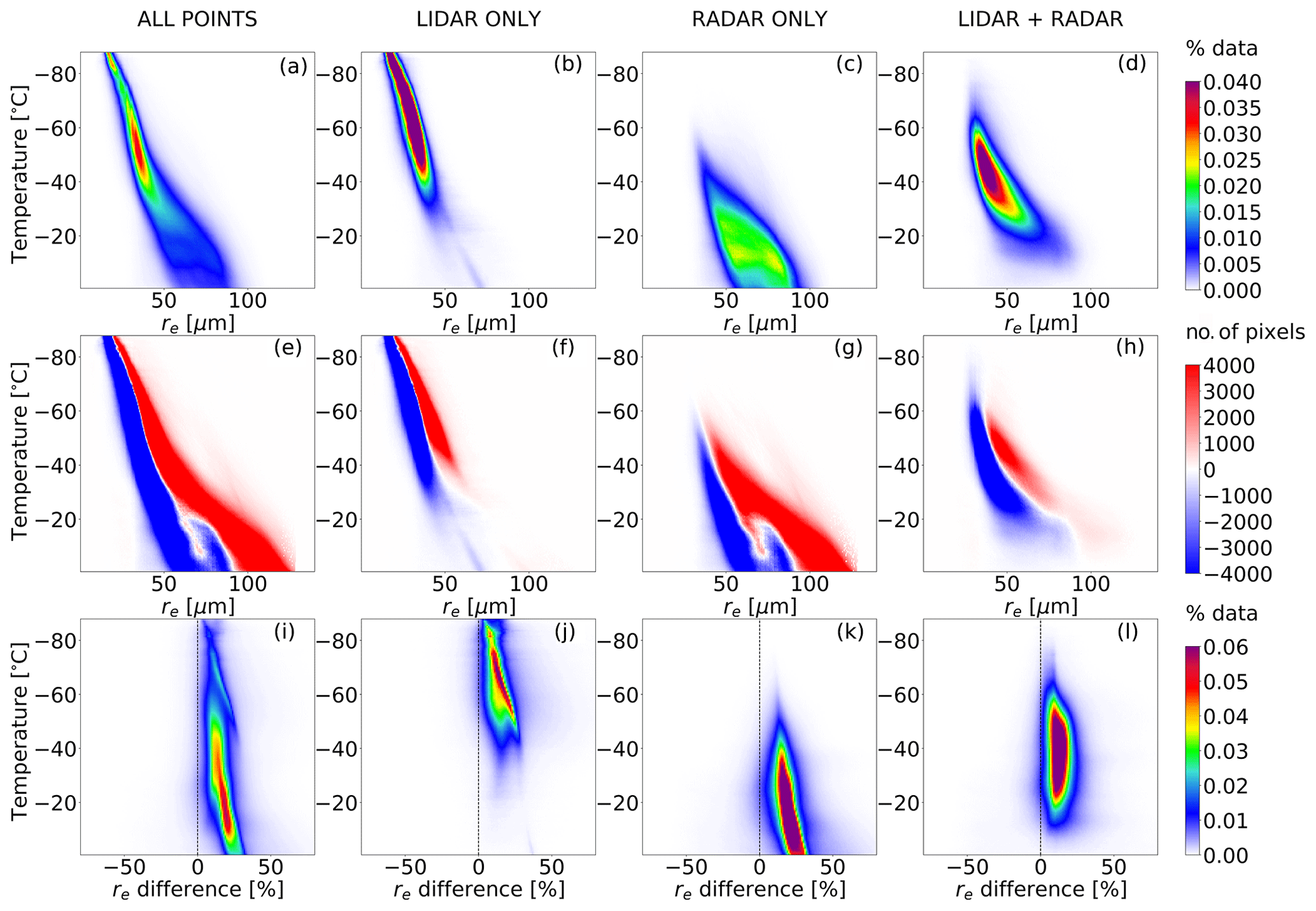
A more detailed comparison is made in Fig. 8. It is clear that IWC tends to increase with temperature as well as its variability (Fig. 8a). For lidar-only pixels, information is mainly available at temperatures below −40 ∘C (Fig. 8b). In most cases, the lidar is strongly attenuated when it penetrates deeper in the cloud to reach higher temperatures. Low-level ice clouds can be detected by the lidar but only if the attenuation is not too strong in the higher levels, which is the case for only a minority of the cloud scenes detected by the CloudSat-CALIPSO instruments. In cold regions detected by the lidar alone, IWC values range from g m−3 for temperatures below −80 ∘C to almost 10−1 g m−3 around −60 ∘C. Radar-only pixels can be found for temperatures above −50 ∘C, where IWC from 10−3 to 1 g m−3 can be observed, especially in the warmest regions where ∘C (Fig. 8c). Finally, synergetic areas are found in between those two regions (Fig. 8d). When looking at the difference between V2 and V3 (Fig. 8e–h), red areas indicate that more pixels from V3 were found to fit in the corresponding [IWC−T] range than from V2. On the contrary, in blue areas, there are fewer pixels from V3. One can see again that the distribution is shifted towards lower values of IWC no matter where in the cloud and which instrument is available. However, the difference is the strongest at the coldest temperatures ( ∘C), which is where we find most of the lidar-only pixels and where the difference between the two lidar ratio a priori relationships is the largest. At warmer temperatures, on the contrary, there is almost no change in the log10(IWC) distribution as the retrieval mainly depends on the radar measurements. Following the behaviour of the lidar ratio, two modes can be distinguished in the distribution of relative difference in IWC as a function of temperature (Fig. 8i–l). Most of the IWC retrievals present differences less than 25 %. However, for temperatures between −50 and −70 ∘C, at which most of the lidar-only pixels can be found, the discrepancies vary between −40 % and −50 % on average.
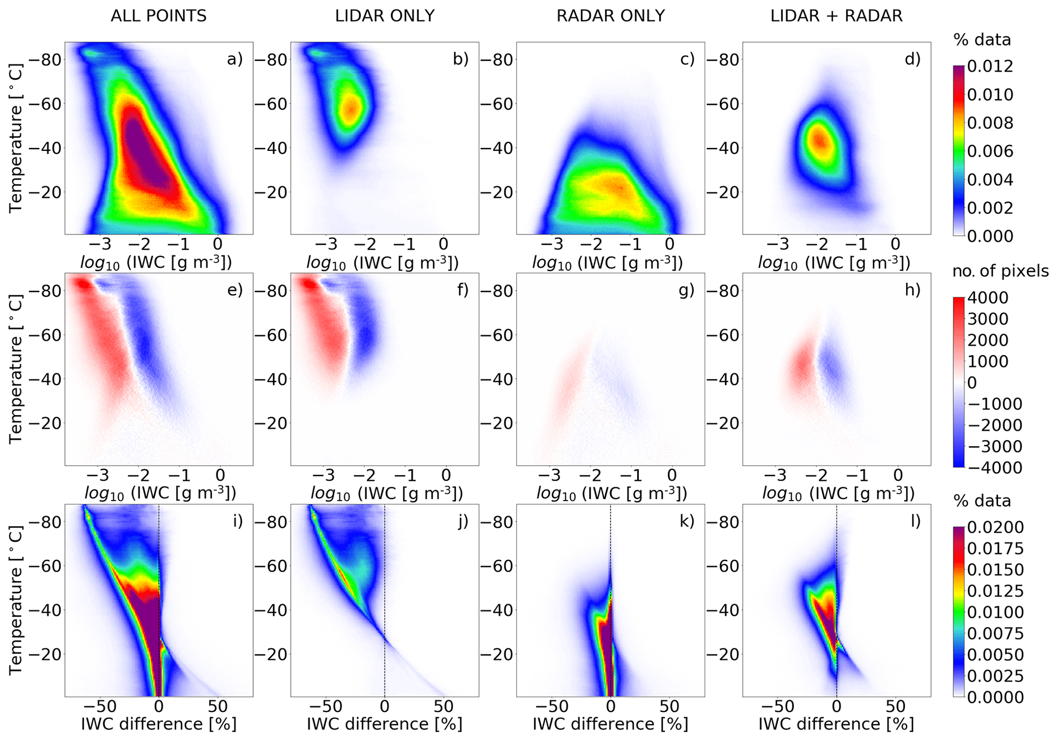
Figure 8Comparison of the retrieved IWC for the V2 and V3 a priori parameterizations of the lidar ratio: probability density distributions of log10(IWC) as a function of temperature obtained when using the new configuration (V3) (a–d), differences in the log10(IWC) distributions in terms of number of retrieved pixels for each [log10(IWC)−T] bin (e–h), and finally the distribution of the relative difference between IWC obtained with the new V3 lidar ratio a priori and IWC obtained with the old V2 configuration, , as a function of temperature (i–l). The first column shows the distributions for all retrieved pixels, the second column, for lidar-only pixels, the third column, for radar-only pixels, and the last column for lidar–radar pixels.
4.3 Impact of the new microphysical model
The analysis of a more recent and larger in situ dataset including bulk IWC measurements allowed the microphysical model to be refined as explained in Sect. 3.2. In this section, we show the consequences of this new parameterization in the IWC retrievals. To do so, the Varcloud algorithm was run using the V2 and V3 LUT and a priori value one after the other, both associated with the V3 lidar ratio a priori. In the same way as for the study on the new lidar ratio a priori, we can look at the differences in the distribution of log10(IWC) (Fig. 9). The impact of the microphysical model is more complex as its action occurs both in the radar forward model and at the end of the process when the IWC is retrieved from extinction and thanks to the 1-D lookup table. Moreover, the interactions that may exist between the parameters that were refined (the PSD, M(D), and a priori value) are likely to have different impacts on the retrieval depending on the physical and microphysical conditions of the observed cloud region. As a result, we will not try to interpret here the differences observed between the two microphysical configurations but describe how the retrieval is impacted.
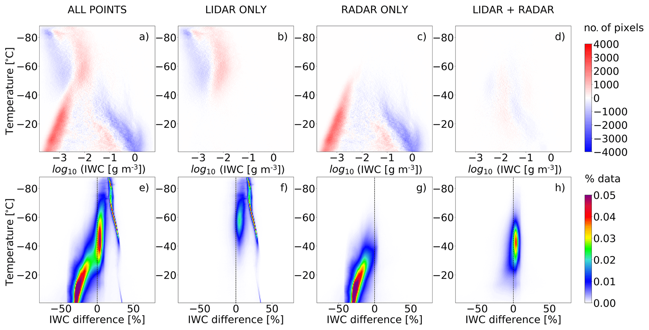
Figure 9Comparison of the retrieved IWC for the two microphysical parameterizations presented in Sect. 3.2 (but with the same lidar ratio a priori). Panels (a)–(d) and (e–h) correspond to panels (e)–(h) and (i–l) of Fig. 8, respectively.
First of all, when looking at Fig. 9a, it seems that the impact of the new microphysics strongly depends on the temperature, with an increase in the averaged retrieved IWC for temperatures below −40 ∘C and a decrease for temperatures above −40 ∘C. When pixels are separated in different regions depending on the available instruments (lidar only, radar only, or both), it is clear that the impact of the new model is also very different for the two instruments: the increase in IWC observed for the cold temperatures is associated with lidar-only pixels (panel b). On the contrary, radar-only pixels are marked by a shift of the distribution towards lower values of IWC (panel c). Where both instruments are available, the opposite effects cancel each other out, which leads to almost no difference in the distribution of log10(IWC) in such regions (panel d). The differences observed in the retrieved IWC in regions detected by the two instruments barely exceed 10 % (panel h). On the contrary, in regions where only one instrument is available, differences are observed between 0 % and 40 % for lidar-only pixels (panel f) and between −40 % and 0 % for radar-only pixels (panel g).
For pixels detected by the lidar only, two modes can be observed in the distribution of the differences between V2 and V3, which overall leads to a decrease in the retrieved ice water path. The main mode is the thin red (strong occurrence) curved line and accounts for profiles for which only the lidar was able to detect a cloud. In such conditions, the extinction is retrieved using the lidar measurement and the lidar ratio a priori. It is therefore completely independent of the microphysical model. The normalized concentration number parameter is then derived using the extinction and the a priori value of . As a result, the retrieved IWC, derived using the extinction and the LUT, depends on the microphysical model in a deterministic way. This curve is the direct translation of the difference between the two configurations into the relationship between visible extinction and IWC as it is parameterized in the LUT. It also illustrates the strong dependency of the microphysical parameterization on the temperature. The second mode presents smaller differences and accounts for the influence of radar measurements deeper in the cloud profile, which balance the increase in IWC by their opposite effect. For radar-only pixels, the influence of the microphysical parameterization is more diffuse as it also plays a role in the iteration process through the radar forward model.
4.4 Conclusions regarding DARDAR-CLOUD new version
4.4.1 IWC retrievals
As a summary of all these modifications in the retrieval code, Fig. 10 presents the difference between the new distribution (V3) of retrieved log10(IWC) and the distribution of DARDAR-CLOUD V2 (panels a to d) as well as the relative differences in IWC between the two versions (panels e to h). The new version includes all the updates presented above. Also taken into account is the update of CALIPSO Level 1 products (v4) consisting of the use of better ancillary datasets: a more accurate DEM (digital elevation model) and a new reanalysis product for the atmospheric variables (MERRA-2), which is shown to allow for more reliable CALIOP calibration coefficients. Information on this update can be found on the NASA website at the following address: https://www-calipso.larc.nasa.gov/resources/calipso_users_guide/data_summaries/l1b/CAL_LID_L1-Standard-V4-10.php (last access: 9 May 2019).
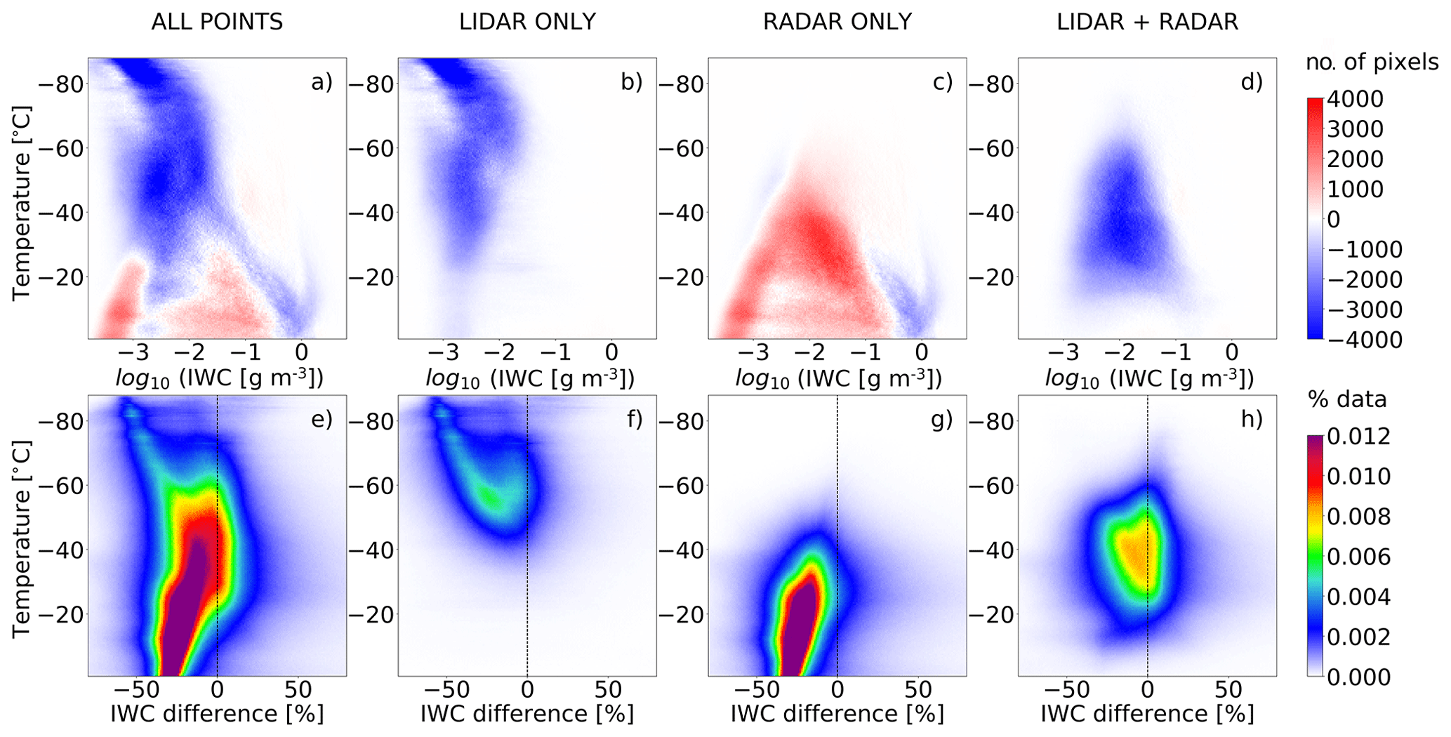
When comparing the two distributions of log10(IWC), we can see that the reduction in the number of retrieved IWC pixels due to the new classification prevails in lidar (panel b) and lidar–radar areas (panel d). On the contrary, in regions where only radar measurements are available, more pixels are retrieved (panel c). Different features can be observed in the relative difference distributions (panels e–h), which are the combination of the updates in the microphysical model that strongly modify the retrievals in the radar-only regions and the impact of the new lidar ratio a priori, mainly affecting the lidar-only and lidar–radar areas. In these areas, the influence of the new LUT is opposed to that of the lidar ratio a priori: the new normalized PSD associated with the choice of the Composite mass–size relationship produces higher values of IWC when lower values of S tend to create lower IWC. It appears, however, that the influence of the lidar ratio prevails, visible in the two modes that can be observed in panel (f), similar to the ones described in Sect. 4.2. The combination of all the modifications made to the retrieval algorithm also seems to create larger differences, positive as well as negative, regardless of the pixel location. However, the probability of occurrence for such values is much lower than for the features previously described. The relative differences shown here are calculated only where ice is detected by both configurations. It is in the synergistic areas that the highest probability is found for the smallest differences.
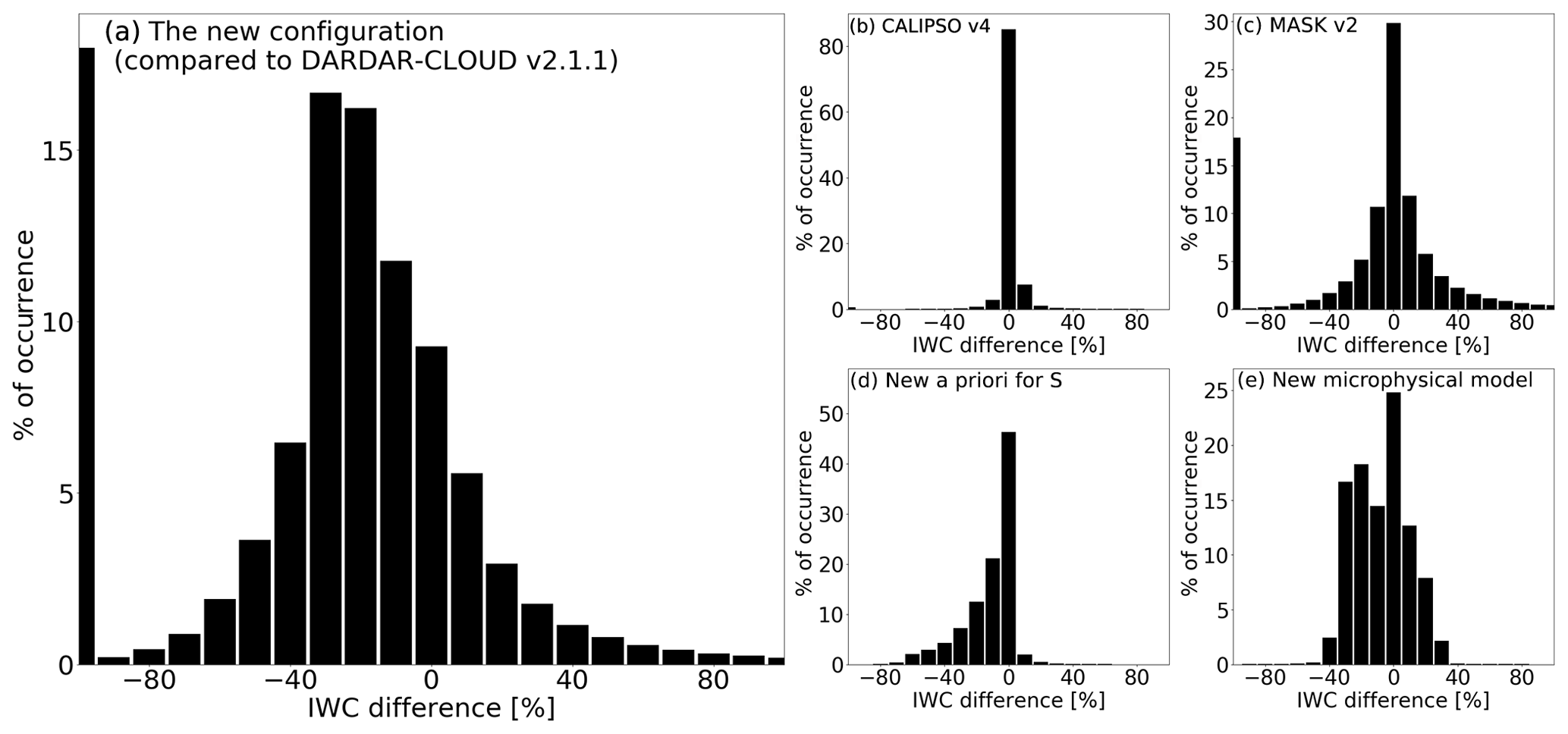
Figure 11Histograms, in percentage of occurrence, of the relative differences in IWC between V2 and V3 (a) and for every modification made in the new version: CALIPSO v4 (b), DARDAR-MASK v2 (c), the new a priori for S (d), and the new lookup table (e).
Figure 11 shows the global histogram of the relative difference in IWC between DARDAR-CLOUD V2 and the new version (a) and the contribution of the different updates. This information was obtained by running the algorithm several times with a different configuration. Each histogram is a comparison between two retrievals, processed with only one modification in the algorithm: changing the version of the CALIPSO Level 1 product (b), the DARDAR-MASK classification product (c), the parameterization of the lidar ratio a priori (d), or the microphysical model (e). When each contribution is taken separately, it can be seen that the highest percentage of occurrence is found for differences <5 %. However, the combination of the new a priori value for the lidar ratio and the new microphysical model leads to an average reduction of −16 % from DARDAR-CLOUD V2 to DARDAR-CLOUD V3. As said previously in Sect. 4.1, the 18 % of the data showing −100 % difference account for the evolution of the hydrometeor classification (Fig. 11a, c). The new updates on CALIPSO product can also modify the classification and the retrieval, although to a lesser extent. Indeed, more than 80 % remain with differences <5 % (Fig. 11b). The largest differences are due to the impact of the new classification, which accounts for the broadening of the probability density observed in Fig. 10. This analysis shows that fewer than 10 % of the data remain with differences <5 %.
4.4.2 re retrievals
Particle size information is given in DARDAR-CLOUD via the retrieved effective radii (re). re is defined as the ratio of IWC and αv:
with ρi the density of solid ice. Figure 12 shows the new distribution (V3) of retrieved re (panels a to d) and its difference with the distribution of DARDAR-CLOUD V2 (panels e to h). The relative differences in re between the two versions are also presented (panels i to l). Similarly to IWC, the effective radius tends to increase with temperature as well as its variability. The influence of temperature is however stronger as the dispersion of the retrieved re is much smaller than that of the retrieved IWC. The new parameterizations clearly impact the retrieved re: the entire distribution as a function of temperature is shifted towards larger values, reaching 140 µm in V3 for the warmest regions, when in V2, the highest value of retrieved re was around 100 µm. This effect is due to the change of microphysical model which has the strongest influence on the retrieval of re. The largest differences (between +20 % and +40 %) are found in the radar-only regions at the warmest temperatures. For pixels that benefit from the combined influence of the two instruments, the impact of the configuration change is reduced (differences are found between +5 % and +25 %).
This paper gives an overview of the main characteristics of the DARDAR-CLOUD new version, describing the modifications made to the Varcloud algorithm and their consequences on the retrieved ice water content. We have shown that the evolution of the DARDAR-CLOUD forward model configuration and the DARDAR-MASK hydrometeor classification could lead to differences in retrieved IWC of up to a factor 2 relative to the earlier release, regardless of the instruments available or the temperature range. These very large discrepancies, which are mainly the consequence of the new phase categorization, represent 5 % of the data used for this study. 90 % of the IWC values show differences less than 50 % with the old configuration. The change in the microphysical model also affects the retrieved re everywhere along the temperature profile, with differences ranging from 5 % to 40 %.
The new values in the parameterization of the lidar extinction-to-backscatter ratio a priori was shown to have little influence on the retrieved re. On the other hand, for IWC retrievals, they have more impact for temperatures below −40 ∘C and induce lower IWC (up to −50 % for the coldest temperatures) in every cloud region detected by the lidar. However, their impact is significantly reduced by the new LUT, which introduces opposite modifications in lidar-only regions. Radar-only regions are mainly influenced by the modifications of the LUT and the a priori value of , which also reduce the values of IWC up to −40 % for the warmest temperatures. In synergistic areas, the combination of the two instruments seems to mitigate the impact of the modifications made in the microphysical model. Nevertheless, differences between −20 % and 20 % are also found in this region between −60 and −20 ∘C. Overall, the new DARDAR-CLOUD version presents retrieved IWC values smaller by 20 %, leading to a reduction in the integrated ice water path (−24 % on average).
Trying to find a simple parameterization of the lidar extinction-to-backscatter ratio was shown to be rather challenging, and uncertainties remain high, particularly in regions where synergies are not available. More work could be done on the subject, adding radiometric instruments or looking at new instrumental platforms, such as the upcoming ESA/JAXA EarthCARE satellite, with a more sensitive radar, and High Spectral Resolution Lidar, which could help refine our analyses.
This sensitivity study was done to help us identify improvements to be considered in the new version that will be made available at the AERIS/ICARE Data and Services Center. Our approach here is to use information and datasets validated by the literature to determine the microphysical assumptions and study the sensitivity of our algorithm to those assumptions. Further improvements are aimed at relying on more in situ and satellite observations to make parameterizations and combination of instruments more efficient, benefiting from CALIPSO-CloudSat extension and EarthCARE advent.
DARDAR-CLOUD retrieval products v2 as well as the DARDAR-MASK v1.1.4 and v2.11 products are publicly available on the AERIS/ICARE website (http://www.icare.univ-lille1.fr/, last access: 11 January 2017). Microphysical data from the ARM program can be found on the ARM archive website (https://www.arm.gov/data, last access: 20 January 2017).
QC and MC performed investigations on possible changes in the new parameters and proposed a new version for the algorithm, with support from JD, JP, and AH. In situ data were provided by AH and satellite data by the AERIS/ICARE Data and Services Center. QC prepared the paper with contributions from all co-authors.
The authors declare that they have no conflict of interest.
Quitterie Cazenave's research is funded by CNES and the DLR/VO-R young investigator group, and we thank the AERIS/ICARE Data and Services Center (http://www.icare.univ-lille1.fr/, last access: 9 May 2019) as well as the CloudSat and CALIPSO projects for providing access to the data used in this study.
This paper was edited by Patrick Eriksson and reviewed by two anonymous referees.
Brown, P. R. A. and Francis, P. N.: Improved measurements of the ice water content in cirrus using a total–water probe, J. Atmos. Ocean. Tech., 12, 410–414, 1995. a, b, c
Ceccaldi, M., Delanoë, J., Hogan, R. J., Pounder, N., Protat, A., and Pelon, J.: From CloudSat-CALIPSO to EarthCare: Evolution of the DARDAR cloud classification and its comparison to airborne radar-lidar observations, J. Geophys. Res.-Atmos., 118, 7962–7981, https://doi.org/10.1002/jgrd.50579, 2013. a, b, c, d
Chen, W., Chiang, C., and Nee, J.: Lidar ratio and depolarization ratio for cirrus clouds, Appl. Optics, 41, 6470–6476, 2002. a
Delanoë, J. and Hogan, R. J.: A variational scheme for retrieving ice cloud properties from combined radar, lidar and infrared radiometer, J. Geophys. Res., 113, D07204, https://doi.org/10.1029/2007JD009000, 2008. a, b
Delanoë, J. and Hogan, R. J.: Combined CloudSat-CALIPSO-MODIS retrievals of the properties of ice clouds, J. Geophys. Res., 115, D4, https://doi.org/10.1029/2009JD012346, 2010. a, b
Delanoë, J., Protat, A., Testud, J., Bouniol, D., Heymsfield, A. J., Bansemer, A., Brown, P. R. A., and Forbes, R. M.: Statistical properties of the normalized ice particle size distribution, J. Geophys. Res., 110, 10201, https://doi.org/10.1029/2004JD005405, 2005. a, b, c
Delanoë, J., Protat, A., Jourdan, O., Pelon, J., Papazzoni, M., Dupuy, R., Gayet, J. F., and Jouan, C.: Comparison of airborne in situ, airborne radar-lidar, and spaceborne radar-lidar retrievals of polar ice cloud properties sampled during the POLARCAT campaign, J. Atmos. Ocean. Tech., 30, 57–73, https://doi.org/10.1175/JTECH-D-11-00200.1, 2013. a
Delanoë, J. M. E., Heymsfield, A. J., Protat, A., Bansemer, A., and Hogan, R. J.: Normalised Particle Size Distribution for remote sensing application, J. Geophys. Res.-Atmos., 119, 4204–4227, https://doi.org/10.1002/2013JD020700, 2014. a, b, c, d, e, f, g, h, i, j
Deng, M., Mace, G., Wang, Z., and Okamoto, H.: Tropical Composition, Cloud and Climate Coupling Experiment validation for cirrus cloud profiling retrieval using CloudSat radar and CALIPSO lidar, J. Geophys. Res.-Atmos., 115, D00J15, https://doi.org/10.1029/2009JD013104, 2010. a
Deng, M., Mace, G., Wang, Z., and Lawson, R. P.: Evaluation of several A-Train ice cloud retrieval products with in-situ measurements collected during the SPARTICUS campaign, J. Appl. Meteorol. Clim., 52, 1014–1030, https://doi.org/10.1175/JAMC-D-12-054.1, 2013. a, b, c
Donovan, D. P., van Lammeren, A. C. A. P., Russchenberg, H. W. J., Apituley, A., Hogan, R. J., Francis, P. N., Testud, J., Pelon, J., Quante, M., and Goddard, J. W. F.: Cloud effective particles size and water content profile retrievals using combined radar and lidar observations – 2. Comparison with IR radiometer and in-situ measurements of ice clouds, J. Geophys. Res., 106, 27449–27464, 2001. a, b
Erfani, E. and Mitchell, D. L.: Developing and bounding ice particle mass- and area-dimension expressions for use in atmospheric models and remote sensing, Atmos. Chem. Phys., 16, 4379–4400, https://doi.org/10.5194/acp-16-4379-2016, 2016. a, b, c, d
Evans, K. F., Wang, J. R., Racette, P. E., Heymsfield, G., and Li, L.: Ice Cloud Retrievals and Analysis with the Compact Scanning Submillimeter Imaging Radiometer and the Cloud Radar System during CRYSTAL FACE., J. Appl. Meteorol., 44, 839–859, https://doi.org/10.1175/JAM2250.1, 2005. a
Garnier, A., Pelon, J., Dubuisson, P., Faivre, M., Chomette, O., Pascal, N., and Kratz, D. P.: Retrieval of cloud properties using CALIPSO Imaging Infrared Radiometer. Part I: effective emissivity and optical depth, J. Appl. Meteorol. Clim., 51, 1407–1425, https://doi.org/10.1175/JAMC-D-11-0220.1, 2012. a
Garnier, A., Pelon, J., Dubuisson, P., Yang, P., Faivre, M., Chomette, O., Pascal, N., Lucker, P., and Murray, T.: Retrieval of cloud properties using CALIPSO Imaging Infrared Radiometer. Part II: effective diameter and ice water path, J. Appl. Meteorol. Clim., 52, 2582–2599, https://doi.org/10.1175/JAMC-D-12-0328.1, 2013. a
Garnier, A., Pelon, J., Vaughan, M. A., Winker, D. M., Trepte, C. R., and Dubuisson, P.: Lidar multiple scattering factors inferred from CALIPSO lidar and IIR retrievals of semi-transparent cirrus cloud optical depths over oceans, Atmos. Meas. Tech., 8, 2759–2774, https://doi.org/10.5194/amt-8-2759-2015, 2015. a, b, c, d, e
Guignard, A., Stubenrauch, C. J., Baran, A. J., and Armante, R.: Bulk microphysical properties of semi-transparent cirrus from AIRS: a six year global climatology and statistical analysis in synergy with geometrical profiling data from CloudSat-CALIPSO, Atmos. Chem. Phys., 12, 503–525, https://doi.org/10.5194/acp-12-503-2012, 2012. a
Heymsfield, A. J., Schmitt, C., Bansemer, A., and Twohy, C. H.: Improved Representation of Ice Particle Masses Based on Observations in Natural Clouds, J. Atmos. Sci., 67, 3303–3318, https://doi.org/10.1175/2010JAS3507.1, 2010. a, b, c, d, e
Heymsfield, A. J., Winker, D., Avery, M., Vaughan, M., Diskin, G., Deng, M., Mitev, V., and Matthey, R.: Relationships between Ice Water Content and Volume Extinction Coefficient from In Situ Observations for Temperatures from 0 ∘C to −86 ∘C: Implications for Spaceborne Lidar Retrievals, J. Appl. Meteorol. Clim., 53, 479–505, https://doi.org/10.1175/JAMC-D-13-087.1, 2014. a
Hogan, R., Francis, P. N., Flentje, H., Illingworth, A., Quante, M., and Pelon, J.: Characteristics of mixed-phase clouds. I: Lidar, radar and aircraft observations from CLARE'98, Q. J. Roy. Meteor. Soc., 129, 2089–2116, https://doi.org/10.1256/rj.01.208, 2003. a
Hogan, R. J.: Fast Lidar and Radar Multiple–Scattering Models. Part I: Small–Angle Scattering Using the Photon Variance–Covariance Method, J. Atmos. Sci., 65, 3621–3635, https://doi.org/10.1175/2008JAS2642.1, 2008. a
Hong, G., Minnis, P., Doelling, D., Ayers, J. K., and Sun-Mack, S.: Estimating effective particle size of tropical deep convective clouds with a look-up table method using satellite measurements of brightness temperature differences, J. Geophys. Res., 117, D06207, https://doi.org/10.1029/2011JD016652, 2012. a
Hong, Y. and Liu, G.: The characteristics of ice cloud properties derived from CloudSat and CALIPSO measurements, J. Climate, 28, 3880–3901, https://doi.org/10.1175/JCLI-D-14-00666.1, 2015. a
Lawson, R. P. and Baker, B. A.: Improvement in determination of ice water content from two-dimensional particle imagery. Part II: Applications to collected data, J. Appl. Meteorol. Clim., 45, 1291–1303, https://doi.org/10.1175/JAM2399.1, 2006. a
Liou, K. N. and Yang, P.: Light Scattering by Ice Crystals: Fundamentals and Applications, Cambridge University Press, Cambridge, UK, 2016. a
Liu, C. L. and Illingworth, A.: Toward more accurate retrievals of ice water content from radar measurements of clouds., J. Appl. Meteorol., 39, 1130–1146, 2000. a
Mishchenko, M. I., Videen, G., Babenko, V. A., Khlebtsov, N. G., and Wriedt, T.: T-matrix theory of electromagnetic scattering by particles and its applications: A comprehensive reference database, J. Quant. Spectrosc. Ra., 88, 357–406, https://doi.org/10.1016/j.jqsrt.2004.05.002, 2004. a
Mitchell, D.: Use of mass- and area-dimensional power laws for determining precipitation particle terminal velocity., J. Atmos. Sci, 53, 1710–1723, 1996. a, b, c
Okamoto, H., Iwasaki, S., Yasui, M., Horie, H., Kuroiwa, H., and Kumagai, H.: An algorithm for retrieval of cloud microphysics using 95-GHz cloud radar and lidar, J. Geophys. Res., 108, 4226–4247, https://doi.org/10.1029/2001JD001225, 2003. a, b
Okamoto, H., Sato, K., and Hagihira, Y.: Global analysis of ice microphysics from CloudSat and CALIPSO: Incorporation of specular reflection in lidar signals, J. Geophys. Res., 115, D22209, https://doi.org/10.1029/2009JD013383, 2010. a
Platt, C. M. R.: Lidar and Radiometric Observations of Cirrus Clouds, J. Atmos. Sci., 30, 1191–1204, https://doi.org/10.1175/1520-0469(1973)030<1191:LAROOC>2.0.CO;2, 1973. a
Platt, C. M. R., Scott, S., and Dilley, A.: Remote Sounding of High Clouds: IV. Optical properties of midlatitude and tropical cirrus, J. Atmos. Sci., 44, 729–747, 1987. a
Platt, C. M. R., Young, S. A., Austin, R. T., Patterson, G. R., Mitchell, D. L., and Miller, S. D.: LIRAD Observations of tropical cirrus clouds in MCTEX. Part I: Optical properties and detection of small particles in cold cirrus, J. Atmos. Sci., 59, 3145–3162, 2002. a, b
Saito, M., Iwabuchi, H., Yang, P., Tang, G., King, M. D., and Sekiguchi, M.: Ice particle morphology and microphysical properties of cirrus clouds inferred from combined CALIOP-IIR measurement, J. Geophys. Res.-Atmos., 122, 4440–4462, https://doi.org/10.1002/2016JD026080, 2017. a
Sourdeval, O., C.-Labonnote, L., Baran, A. J., and Brogniez, G.: A methodology for simultaneous retrieval of ice and liquid water cloud properties. Part 1: Information content and case study, Q. J. Roy. Meteor. Soc., 141, 870–882, https://doi.org/10.1002/qj.2405, 2014. a
Sourdeval, O., C.-Labonnote, L., Baran, A. J., Mülmenstädt, J., and Brogniez, G.: A methodology for simultaneous retrieval of ice and liquid water cloud properties. Part 2: Near-global retrievals and evaluation against A-Train products, Q. J. Roy. Meteor. Soc., 142, 3063–3081, https://doi.org/10.1002/qj.2889, 2016. a, b
Stephens, G. L., Vane, D. G., Boain, R. J., Mace, G. G., Sassen, K., Wang, Z., Illingworth, A. J., O'Connor, E. J., Rossow, W. B., Durden, S. L., Miller, S. D., Austin, R. T., Benedetti, A., Mitrescu, C., and the CloudSat Science Team: The CloudSat Mission and the A-Train, B. Am. Meteorol. Soc., 83, 1771–1790, https://doi.org/10.1175/BAMS-83-12-1771, 2002. a
Stubenrauch, C. J., Holz, R., Chédin, A., Mitchell, D. L., and Baran, A. J.: Retrieval of cirrus ice crystal sizes from 8.3 and 11.1 µm emissivities determined by the improved initialization inversion of TIROS-N Operational Vertical Sounder observations, J. Geophys. Res., 104, 793–808, 1999. a
Thorsen, T. J. and Fu, Q.: Automated Retrieval of Cloud and Aerosol Properties from the ARM Raman Lidar. Part II: Extinction, J. Atmos. Ocean. Tech., 32, 1999–2023, https://doi.org/10.1175/JTECH-D-14-00178.1, 2015. a
Tinel, C., Testud, J., Hogan, R. J., Protat, A., Delanoë, J., and Bouniol, D.: The retrieval of ice cloud properties from cloud radar and lidar synergy, J. Appl. Meteorol., 44, 860–875, 2005. a
Vaughan, M., Young, S., Winker, D., Powell, K., Omar, A., Liu, Z., Hu, Y., and Hostetler, C.: Fully automated analysis of space-based lidar data: an overview of the CALIPSO retrieval algorithms and data products., Proc. SPIE, 5575, 16–30, 2004. a
Wang, Z. and Sassen, K.: Cirrus cloud microphysical property retrieval using lidar and radar measurements – 1. Algorithm description and comparison with in situ data, J. Appl. Meteorol., 41, 218–229, 2002. a
Whiteman, D. N., Demoz, B., and Wang, Z.: Subtropical cirrus cloud extinction to backscatter ratios measured by Raman Lidar during CAMEX-3, Geophys. Res. Lett., 31, L12105, https://doi.org/10.1029/2004GL020003, 2004. a
Winker, D., Hunt, W., and McGill, M. J.: Initial performance assessment of CALIOP, Geophys. Res. Lett., 34, L19803, https://doi.org/10.1029/2007GL030135, 2007. a
Winker, D. M., Pelon, J., Coakley, J. A., Ackerman, S. A., Charlson, R. J., Colarco, P. R., Flamant, P., Fu, Q., Hoff, R. M., Kittaka, C., Kubar, T. L., Treut, H. L., McCormick, M. P., Mégie, G., Poole, L., Powell, K. A., Trepte, C., Vaughan, M. A., and Wielicki, B. A.: The CALIPSO Mission: A global 3D view of aerosols and clouds, B. Am. Meteorol. Soc., 91, 1211–1229, https://doi.org/10.1175/2010BAMS3009.1, 2010. a
Yorks, J. E., Hlavka, D. L., Hart, W. D., and McGill, M. J.: Statistics of cloud optical properties from airborne lidar measurements, J. Atmos. Ocean. Tech., 28, 869–883, https://doi.org/10.1175/2011JTECHA1507.1, 2011. a