the Creative Commons Attribution 4.0 License.
the Creative Commons Attribution 4.0 License.
 | 06 Jun 2019
Revisiting particle sizing using greyscale optical array probes: evaluation using laboratory experiments and synthetic data
Sebastian J. O'Shea
Jonathan Crosier
James Dorsey
Waldemar Schledewitz
Ian Crawford
Stephan Borrmann
Richard Cotton
Aaron Bansemer
In situ observations from research aircraft and instrumented ground sites are important contributions to developing our collective understanding of clouds and are used to inform and validate numerical weather and climate models. Unfortunately, biases in these datasets may be present, which can limit their value. In this paper, we discuss artefacts which may bias data from a widely used family of instrumentation in the field of cloud physics, optical array probes (OAPs). Using laboratory and synthetic datasets, we demonstrate how greyscale analysis can be used to filter data, constraining the sample volume of the OAP and improving data quality, particularly at small sizes where OAP data are considered unreliable. We apply the new methodology to ambient data from two contrasting case studies: one warm cloud and one cirrus cloud. In both cases the new methodology reduces the concentration of small particles (<60 µm) by approximately an order of magnitude. This significantly improves agreement with a Mie-scattering spectrometer for the liquid case and with a holographic imaging probe for the cirrus case. Based on these results, we make specific recommendations to instrument manufacturers, instrument operators and data processors about the optimal use of greyscale OAPs. The data from monoscale OAPs are unreliable and should not be used for particle diameters below approximately 100 µm.
- Article
(3090 KB) - Full-text XML
- BibTeX
- EndNote


Optical array probes (OAPs) are widely used to provide in situ measurements of cloud particle size, habit and concentration (Wendisch and Brenguier, 2013). These measurements provide insights into key cloud microphysical processes such as ice nucleation, particle growth and precipitation (Field, 1999; Lawson et al., 2015). In situ measurements are an important means to constrain remote sensing retrievals, which are routinely used to initialise operational weather forecast models (Fox et al., 2019; Mace and Benson, 2017).
OAPs consist of a laser illuminating a linear array of photodiodes. A particle crossing the laser beam is detected if the laser intensity at any of the elements of the array drops below a threshold value. A shadow image is constructed by appending consecutive slices from the detectors as the particle moves perpendicular to the laser beam.
Monoscale OAPs use a 50 % decrease in signal intensity as their threshold for detection (Knollenberg, 1970; Lawson et al., 2006), resulting in 1 bit binary images with pixels either in an active state or an inactive state. Greyscale OAPs are also available, which detect particles at multiple intensity thresholds, resulting in 2 bit images with pixels having three different active states and one inactive state. For example, a greyscale probe could be configured to record images with pixels off (inactive) or triggered at shadow intensity levels of 25 %, 50 % and 75 %. We use the abbreviations A25−50, A50−75 and A75−100 for the number of pixels associated with decreases in detector signal of 25 %–50 %, 50 %–75 % and 75 %–100 %, respectively. Similarly we use the abbreviations D25, D50 and D75 for the diameters of images with decreases in detector signal greater than 25 %, 50 % and 75 %, respectively. Korolev et al. (1991) describes a hybrid mono-grey system for the closely related 1-D type of probe: this used a similar array to an OAP to size particles using a 50 % shadow intensity but also had on-board signal processing to provide additional filtering and the requirement for at least 1 pixel in any measured image to have a shadow intensity > 67 %. This resulted in the reduction of artefacts due to poorly imaged particles near the edges of the depth of field.
Particles which are imaged by an OAP are fully in focus at the object plane, with image quality deteriorating as the particle location moves away from this object plane. The distance from the object plane at which a particle can be observed is known as the depth of field (DoF) and is used to determine the instruments sample volume (together with the airspeed and effective optical array width). Previous studies have found that the depth of field (at the 50 % intensity level) follows a relationship of the form (Knollenberg, 1970)
where D0 is the particle diameter and λ is the laser wavelength. c is a dimensionless constant, typically between 3 and 8 (Lawson et al., 2006; Gurganus and Lawson, 2018).
The size of the measured image depends on the particle's distance from the object plane. However, this dependence has been shown to be non-monotonic (Joe and List, 1987). Korolev et al. (1991) show that OAP images of transparent spheres (e.g. liquid drops) can be accurately approximated by the Fresnel diffraction from an opaque disc. The ratio of the detected image diameter to the actual physical diameter D0 is purely a function of the normalised, dimensionless distance from the object plane Zd:
where Z is the distance from the object plane. The spatial intensity distributions from transparent spheres are independent of particle size. A distinct feature of these distributions is a bright spot at the centre of the image known as the Poisson spot. Korolev et al. (2007, hereafter K07) describes a method for determining a spherical particle's distance from the object plane and size using the size of the Poisson spot.
Joe and List (1986) suggested significantly reducing the depth of field so that the image size could be assumed to be equal to the particle size. Particles outside the new depth of field were identified using the ratio ). The disadvantage of reducing the depth of field in this way is that it can lead to poor sampling statistics. Korolev et al. (1991) removes the most severely mis-sized particles, by requiring at least 1 pixel to have a > 67 % decrease in detector signal. Reuter and Bakan (1998, hereafter RB98) suggested an alternative approach by assuming a linear relationship between image size and the greyscale ratio ), which they then use to determine the particle size. This relationship was determined using laboratory experiments with a rotating disk with printed circular spots.
This paper describes tests on a Droplet Measurement Technologies Inc. (DMT) greyscale cloud imaging probe (CIP-15) using a droplet generation system. Liquid drops were injected into the probe at measured distances from the object plane to examine how this impacts the ability of the probe to accurately size particles. Results from these experiments are compared to synthetic images calculated assuming Fresnel diffraction (Korolev et al., 1991). Section 3.1 evaluates the efficacy of the K07 and RB98 size correction algorithms. Section 3.2 uses greyscale intensity ratios to determine a particle's distance from the object plane near the edge of the probe's depth of field. This allows significantly fragmented images to be removed and a revised depth of field to be used to determine particle concentrations. Section 3.4 examines how these results impact field measurements of particle size distributions using two research flights: one in a warm liquid cloud and one in cirrus.
Table 1 summarises the main instrumental and experimental characteristics of the laboratory, model and airborne measurements presented in this paper.
Table 1A summary of the main instrumental and experimental characteristics of the laboratory, model and airborne measurements.
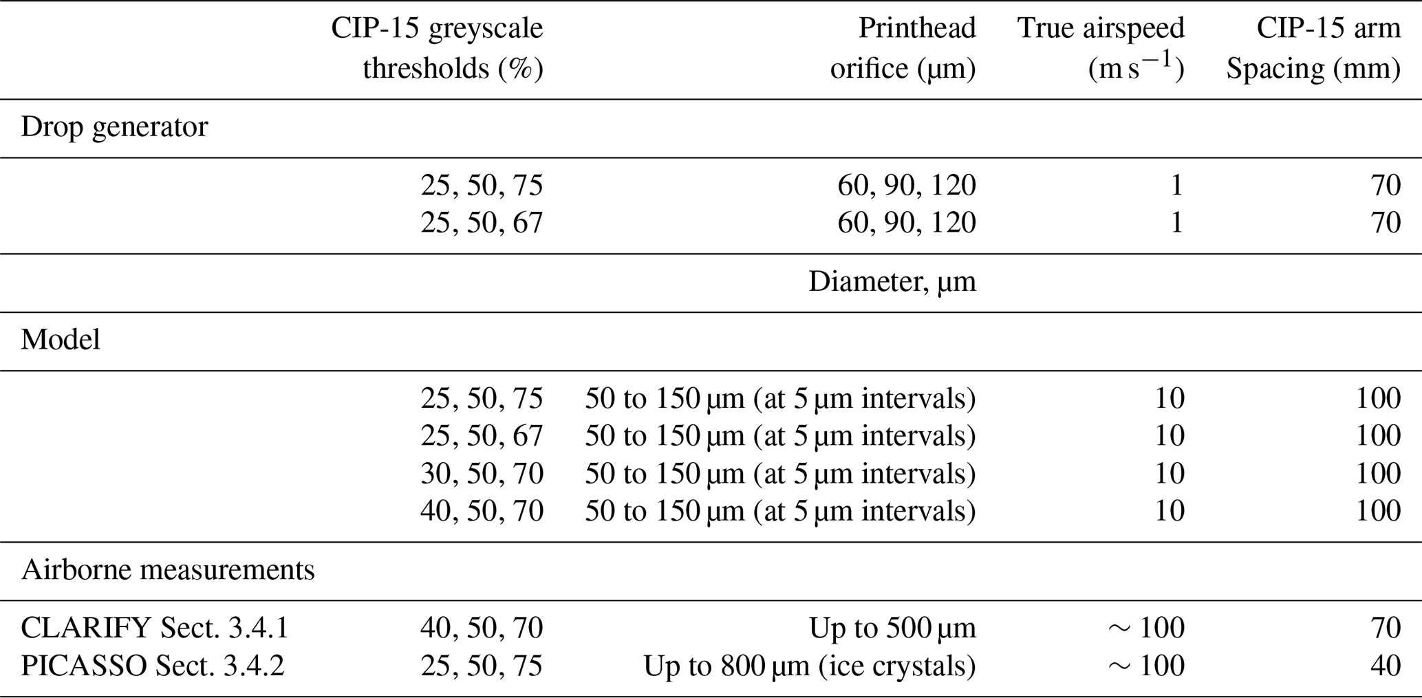
2.1 Cloud imaging probe (CIP-15)
The CIP-15 is a commercially available greyscale OAP (DMT Inc., USA; Baumgardner et al., 2001). It has a 64-element photodiode array with an effective pixel size of 15 µm, giving the probe a nominal size range of 15 to 960 µm. Images are recorded at three greyscale thresholds, which can be varied in the probe's data acquisition software. For the drop generator experiments these thresholds were set to the manufacturer default settings of 25 %, 50 % and 75 % and also 25 %, 50 % and 67 %. In Sect. 3.4.1 the thresholds were 40 %, 50 % and 70 %, and in Sect. 3.4.2 they were 25 %, 50 % and 75 %. The probe is fitted with anti-shatter tips to minimise ice shattering on the leading edge of the probe during field measurements. The measurements presented in this paper are from two CIP-15 systems. The major difference between the two probes is that one CIP-15 has an arm separation of 7 cm, and the other has an arm separation of 4 cm. The laboratory experiments and warm cloud results in Sect. 3.4.1 used the CIP with 7 cm arm separation, whereas the cirrus results in Sect. 3.4.2 use the CIP with 4 cm arm separation.
2.2 Supporting measurements
Section 3.4 compares measurements from the CIP-15 on board the FAAM Bae-146 research aircraft to those from a DMT Inc. Cloud Droplet Probe (CDP) and a holographic imaging probe. The CDP sizes particles in the range 3 to 50 µm using the scattered light intensity from particles crossing a diode laser and assuming Mie-scattering theory (Lance et al., 2010). The probe was calibrated during the campaign using glass calibration beads.
HALOHolo is a holographic imaging probe from the Institute for Atmospheric Physics at the University of Mainz and Max Planck Institute for Chemistry Mainz. It has a 6576×4384 pixel CCD detector with an effective pixel size of 2.95 µm. This equates to a sample volume of approximately mm (∼38 cm3). At 6 frames per second and an average airspeed of about 100 ms−1, this equates to a volume sample rate of ∼230 cm3 s−1. Particles between 6 µm (2 pixels) and 1 cm (half the detector width) are resolvable in the hologram reconstructions. However, the detection of small particles is limited by noise in the background image. Therefore a minimum size threshold of 35 µm is applied, above which it is estimated that the probe's detection rate is greater than 90 % (Schlenczek, 2017). Shattered particles were minimised by removing all particles with inter-particle distances of less than 10 mm (Fugal and Shaw, 2009; O'Shea et al., 2016).
2.3 Drop generator
A monodisperse stream of droplets was generated using a commercially available droplet generator. The generator is similar to that described by Lance et al. (2010) and uses piezoelectrically actuated printheads. Three MicroFab, Inc (USA) printheads with 60, 90 and 120 µm orifices were used during these experiments (part numbers MJ-ABL-01-60-8MX, MJ-ABL-01-90-8MX and MJ-ABL-01-120-8MX). Each printhead was in turn vertically mounted on two perpendicularly positioned translation stages (MTS50/M-Z8 – 50 mm, Thorlabs), and each has 50 mm travel range and a 0.05 µm minimum increment. The printheads were connected to a fluid reservoir and the fluid pressure was adjusted using a pneumatic pressure controller so that the meniscus was at the end of the printhead. The printheads were actuated using a JetDrive III electronics module (MicroFab, Inc) to give a droplet production rate of 50 Hz.
The generation of a stable stream of monodisperse droplets depends on several factors, including the drive electronics and the physical properties of the fluid used. These factors, together with the size of the printhead orifice, control the size of the generated droplets. Previous work has shown that more stable outputs can be achieved using mixtures of water and ethylene glycol compared to using pure water (Jang et al., 2009; Liu, 2016). For these experiments, with the 60 µm printhead a 50 % water and 50 % ethylene glycol solution was used, while 100 % ethylene glycol was used with the 90 and 120 µm printheads.
Figure 1 shows the setup for experiments that were performed on the CIP-15. The CIP-15 was vertically mounted below the drop generator. For each printhead the drop generator's position was stepped in 0.5 mm increments between the CIP-15's arms, dwelling for 3 s after each movement.
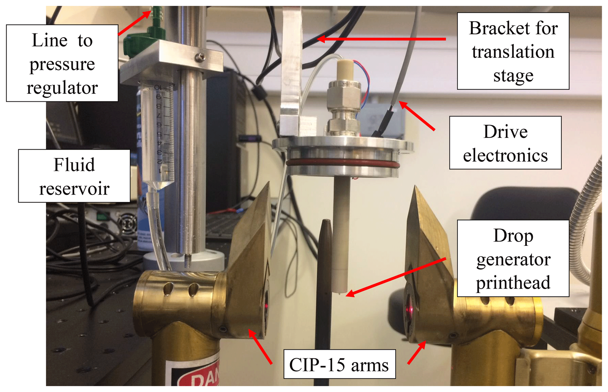
Figure 1A photograph of the droplet generator injecting droplets into the sample volume of the CIP-15.
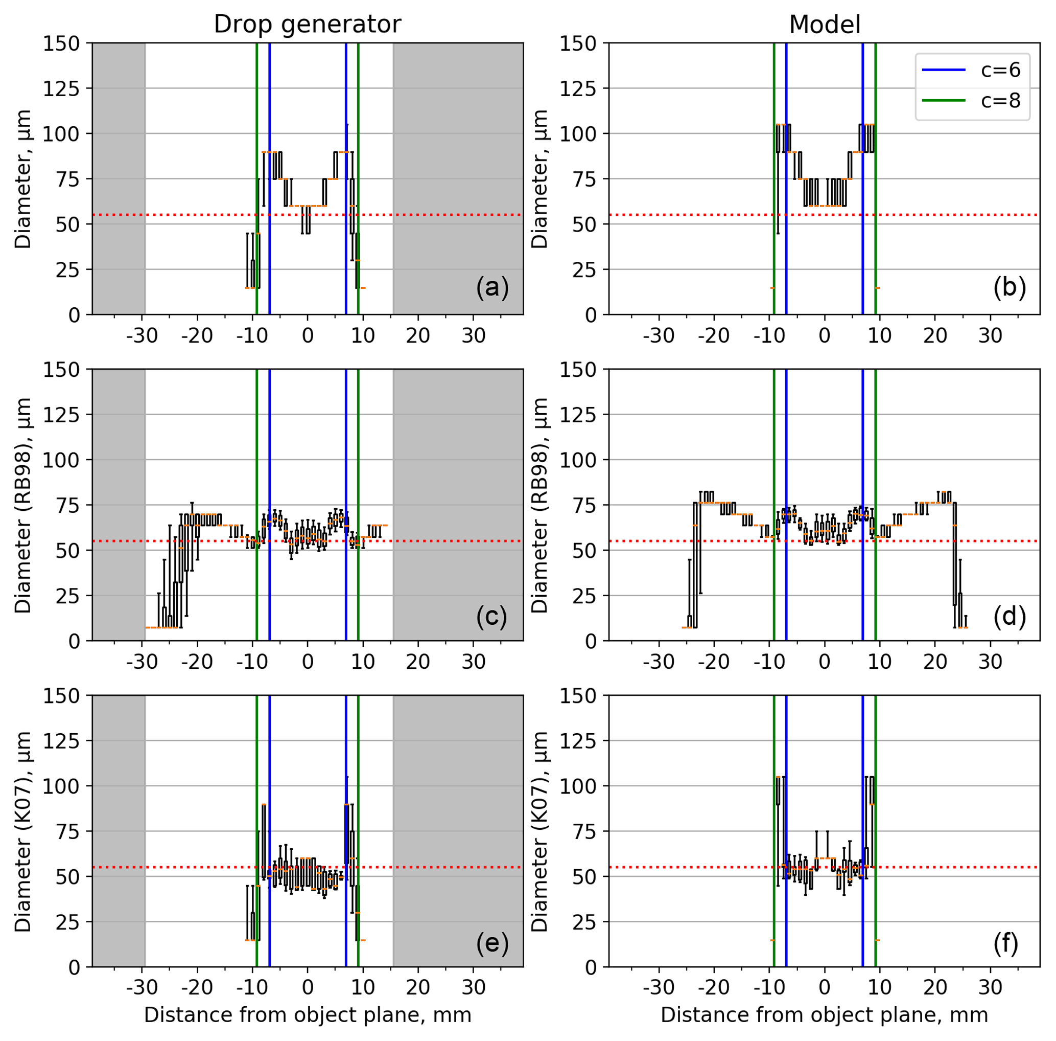
Figure 2Box and whisker plots showing image diameter as a function of distance from the object plane. Orange markers are the median diameter, boxes are the 25 and 75th percentiles and the whiskers are the 10 and 90th percentiles. Panels (a), (c) and (e) show results from the laboratory experiments using a 60 µm printhead. The grey-shaded regions were not sampled using the drop generator. Panels (b), (d) and (f) show the model image diameter from a 55 µm particle. Panels (a) and (b) show the image diameter using a 50 % decrease in intensity threshold (D50). Panels (c) and (d) show the diameter after the Reuter and Bakan (1998) size correction has been applied. Panels (e) and (f) show the diameter corrected using the Korolev et al. (2007) algorithm. Dashed red lines show the droplet diameter estimated by comparing the laboratory measurements with the synthetic data. The position of the depth of field calculated using Eq. (1) with c values of 6 (blue) and 8 (green) are shown as vertical lines.
To test the stability of the droplet generator, separate experiments were performed where the droplets were monitored using a high-speed camera (FASTCAM Mini AX, Photron, UK) with a zoom lens (Navitar, USA). The pixel size (1.4 µm per pixel) of the image for a given magnification was calibrated using a stage graticule (50×2 µm, Graticules Ltd, London, UK). The droplets were monitored for a 1 h period at a droplet production rate of both 10 and 250 droplets s−1. The interquartile ranges of the drop diameters, as measured by the camera, were 2 and 3 µm, respectively. Droplet velocity was typically of the order of 1 m s−1 (±0.5 m s−1).

Figure 3Same as Fig. 2 but panels (a), (c) and (e) show results from the laboratory experiments using a 90 µm printhead and panels (b), (d) and (f) show the modelled image diameter from an 80 µm particle.
2.4 Synthetic data
Modelled images were generated using optical, electronic and diode thresholding simulations. The optical simulation considers only Fresnel diffraction by a round object, following the methods of Korolev et al. (1991) and K07. An electronic time delay simulation was also performed (Baumgardner and Korolev, 1997), but the effects are negligible due to the fast response of the electronics (tau = 51 ns) and the slow speed of the simulation (airspeed of 10 m s−1). The photodiodes are assumed to have a rectangular shape with a 5:4 aspect ratio and a 20 % spacing between them, as in Korolev (2007). Similar to the drop generator experiments, particles were injected at known distances from the object plane and the probe's response was simulated. This was done for particles with diameters 50 to 150 µm at intervals of 5 µm. These were positioned at 1 mm intervals over the range −5 to +5 cm from the object plane. Images were simulated using four different combinations of greyscale thresholds: 25 %, 50 % and 75 %; 30 %, 50 % and 70 %; 40 %, 50 % and 70 %; and 25 %, 50 % and 67 %.

Figure 4Same as Fig. 2 but panels (a), (c) and (e) show results from the laboratory experiments using a 120 µm printhead and panels (a), (c) and (e) show the modelled image diameter from a 90 µm particle.
3.1 Particle size correction
Figures 2–4 show the image diameter as a function of distance from the object plane. Panels (a)–(b) show the image diameter using a 50 % intensity threshold for detection calculated along the axis of the optical array. Panels (a), (c) and (e) of Figs. 2–4 show results from the laboratory experiments using the 60, 90 and 120 µm drop generator printheads, respectively. Example images from the 90 µm printhead at three distances from the object plane are shown in Fig. 5. The image diameter is symmetrical about the object plane with a broad trend of increasing size with distance from the object plane (panels a–b of Figs. 2–4). This occurs until near the edge of the depth of field the image fragments and its size decreases dramatically until it is no longer visible. Theoretically the size of the image at the centre of the object plane should be the closest approximation to the drop size. The median sizes of these are 60, 90 and 90 µm for the 60, 90 and 120 µm printheads, respectively. These measurements are subject to a 15 µm uncertainty due to the pixel resolution of the CIP-15. Based on this and also by comparing them with the synthetic data we estimate the true sizes of the droplets to be 55, 80 and 90 µm (dashed red lines) for the 60, 90 and 120 µm printheads, respectively. Panels (b), (d) and (f) show similar plots for the synthetic data for these sizes. These sizes were chosen as they were the closest match to the droplet calibrations. The position of the depth of field as calculated using Eq. (1) with c values of 6 (blue) and 8 (green) are shown as vertical lines. If calculated correctly particles should not be visible outside the depth of field. If not removed, such particles would bias the measured concentrations. Figures 2–4 show that a c value of 8 effectively bounds the region where particles are visible using a 50 % intensity threshold. The drop velocity will have an impact on this due to the probe's electronic time delay (Baumgardner and Korolev, 1997). These tests were performed with relatively slow droplet velocities (< 10 m s−1), especially when compared to aircraft measurements (approximately 100 m s−1). However, this effect is minimised by the fast time response of modern probes such as the CIP-15 (tau = 51 ns).
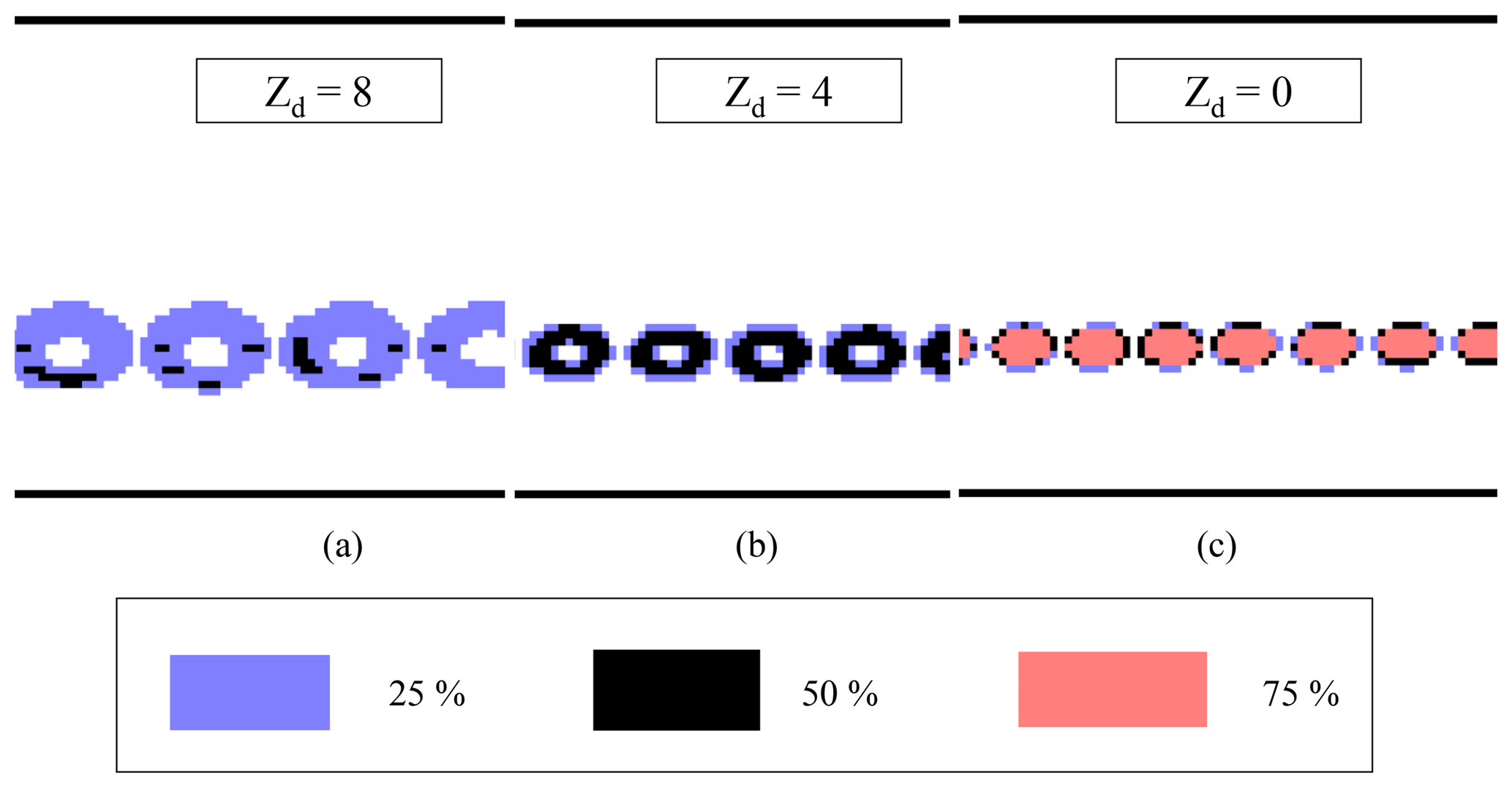
Figure 5Example images from the CIP-15 of droplets from the droplet generator using a 90 µm printhead at Zd=8 (a), Zd=4 (b) and Zd=0 (c). Decreases in detector intensity of 25 % to 50 %, 50 % to 75 % and > 75 % are shown as light blue, black and orange pixels, respectively.
Table 2Median (interquartile range) image diameter for Zd<6 from the drop generator experiments and the model images.
Panels (c)–(d) of Figs. 2–4 show the image diameter as a function of distance from the object plane once the RB98 size correction algorithm has been applied. This algorithm assumes a linear relationship between D25 and the greyscale ratio ). In reality this relationship is not completely linear: as a result the corrected diameter is not independent of position. Additionally there is a bias in the corrected size when compared to the particle model. To quantify this for the synthetic data we calculate the median of each position bin, Table 2 shows statistics for Zd < 6. It is clear that the RB98 algorithm has a bias of the order 10 µm. A similar bias is seen in RB98 when compared to K07 if both algorithms are applied to results from the drop generator (Table 2).
Panels (e)–(f) of Figs. 2–4 show the image diameter after the K07 algorithm has been applied. Across much of the depth of field this algorithm removes the image diameter's position dependence. For the synthetic data the median diameter across the depth of field is now within 1 µm of the true particle diameter and the interquartile range is reduced (Table 2). At the edge of the depth of field the Poisson spots become sufficiently large that the outer ring fragments at the 50 % threshold (Fig. 5a). Once this happens the K07 algorithm is not able to correct the size of these severely misshapen images. As shown in Figs. 2–4 these fragmented images have large variability in their size and can be either much larger or smaller than the true particle size.
3.2 Identifying fragmented images
The K07 algorithm effectively corrects the diameter of imaged spherical particles across much of the depth of field for binary images at the 50 % threshold. However for Zd greater than approximately 7 the images are too fragmented and the correction no longer works effectively. These fragmented images need to be removed from further analysis; otherwise they will bias the measured size distributions.
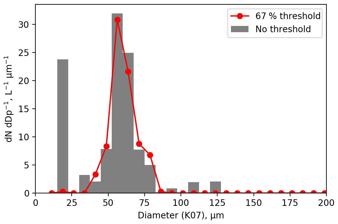
Figure 6Size distribution of the K07-corrected diameter for a drop generator scan using the 60 µm printhead. The grey bars show data from all droplets, while the red markers show only images with at least 1 pixel with a > 67 % decrease in detector intensity. This reduces the depth of field to Zd<4.8.
The 1-D probes described by Korolev et al. (1991) have an element of greyscale filtering. They do not record particle images; rather they just measure the diameter of particles using a 50 % threshold. Only particles that have at least one detector with a > 67 % drop in detector intensity are recorded. To test the efficacy of this approach to remove fragmented particles drop generator scans were performed with the CIP-15 thresholds set to 25 %, 50 % and 67 %. Figure 6 shows a size distribution of the K07-corrected diameter for a scan using the 60 µm printhead. The grey bars show data from all droplets, while the red markers show only images with at least 1 pixel above the 67 % threshold. By performing this filtering the fragmented images are minimised and the depth of field is constrained to Zd < 4.8.
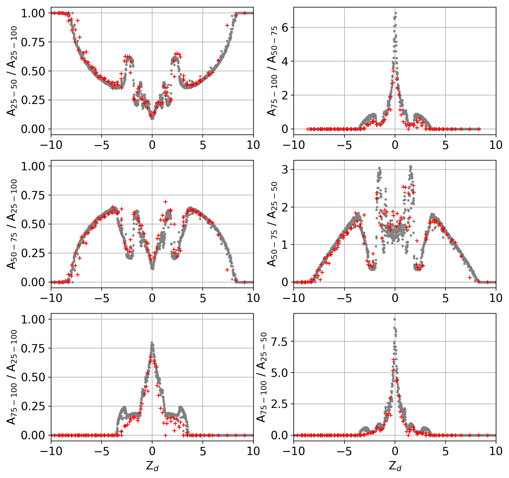
Figure 7The ratios of the number of pixels between different thresholds from the drop generator experiments (red) and model simulations of particles in the size range 50 to 150 µm (grey) as a function of normalised distance from the object plane (Zd).
Ideally greyscale information could be used to uniquely determine a particle's Zd, which could either be used to correct the image size or exclude fragmented images from further analysis. Figure 7 shows various combinations of greyscale ratios as a function of Zd. Results from the model for the particle sizes 50 to 150 µm are shown in grey, while results from the drop generator for the three printhead sizes (60, 90 and 120 µm) are shown in red. None of these ratios are monotonic and most exhibit very complex behaviour. As a consequence they cannot easily be used to determine a particle's position across the whole depth of field. However, within certain regions some of the ratios are monotonic.
The ratio (middle right panel) is near linear for the approximate range . This is an important region since it is where the images begin to fragment and the true particle size can no longer be accurately retrieved using the K07 algorithm. Before this ratio can be used to determine a particle's position, we need to check that is within the linear region. If an image has , then can be limited to less than approximately 3.5. Similarly, if A50−75 is equal to zero, then will be greater than approximately 8.5 and likely too fragmented for accurate sizing.
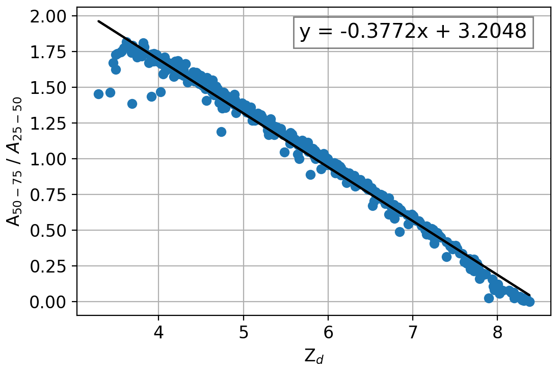
Figure 8The ratio of the number of pixels between greyscale thresholds 50 %–75 % and 25 %–50 % (positive Zd) that meet the criteria and (blue markers). These data are from model simulations of spherical particles in the size range 50 to 150 µm.
Figure 8 shows results from the model (positive Zd) that meet the criteria and (blue markers). The following equation can be fit to the data with an R2 of 0.98:
Equation (3) allows the particle position to be retrieved over the approximate range . It should be noted that the uncertainty is greater for particles in the region due to the larger number of outliers.
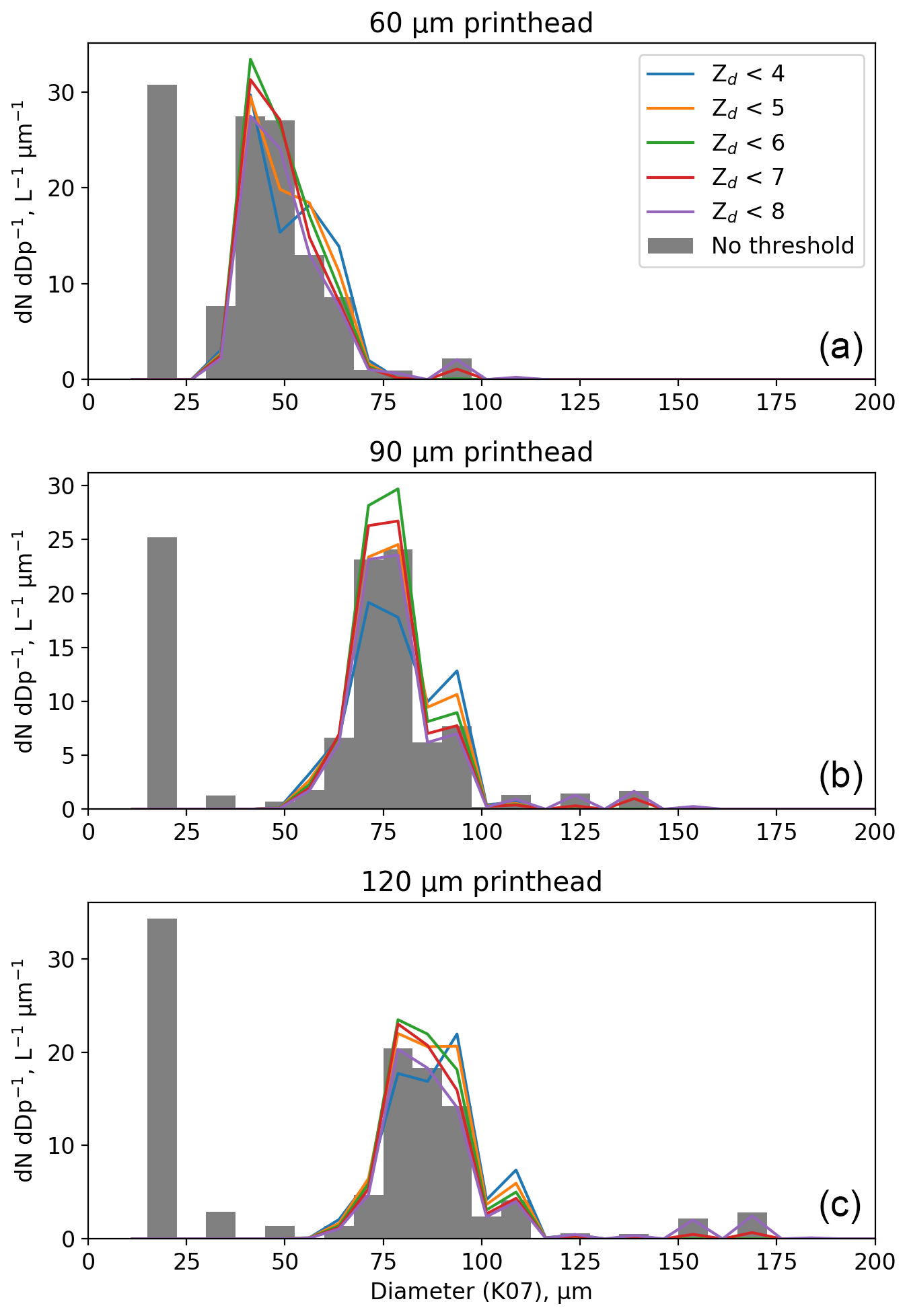
Figure 9Size distributions of the K07-corrected diameter for drop generator scans of the CIP-15 using the 60 µm (a), 90 µm (b) and 120 µm (c) printheads. The grey bars show data from all droplets, while the coloured lines show size distributions that have been filtered using different Zd thresholds. The Zd of each droplet was determined using Eq. (3).
Figure 9 shows size distributions of the K07-corrected diameter for drop generator scans using the 60 µm (Fig. 9a), 90 µm (Fig. 9b) and 120 µm (Fig. 9c) printheads. The grey bars show data from all droplets, while the coloured lines show size distributions that have been filtered using different Zd thresholds. The Zd of each droplet was determined using Eq. (3). By applying a Zd threshold, both the very large and very small outliers are removed from the size distribution.
Similar relationships to Eq. (3) can be derived using different greyscale thresholds. We tested several different combinations of thresholds that could be used: first 40 %, 50 % and 70 %; second 30 %, 50 % and 70 %; and finally 25 %, 50 % and 67 %. A similar procedure was employed of first removing particles with pixels above the highest threshold (AHigh>0) and ones without at least 1 pixel above the middle threshold (AMid=0). For each particle the number of pixels with greyscale intensity between the middle and upper threshold (AMid) was divided by the number of pixels between the lower and middle thresholds (ALow). A linear equation of the following form was then fit to this ratio vs. Zd:
Table 3 shows the fit coefficients for the four different combinations of greyscale thresholds from the model data. Also shown is the approximate Zd range where each relationship is applicable. All four combinations of thresholds were found to have comparable efficacy.
Table 3Fit coefficients i and j for Eq. (4) for different combinations of greyscale thresholds.
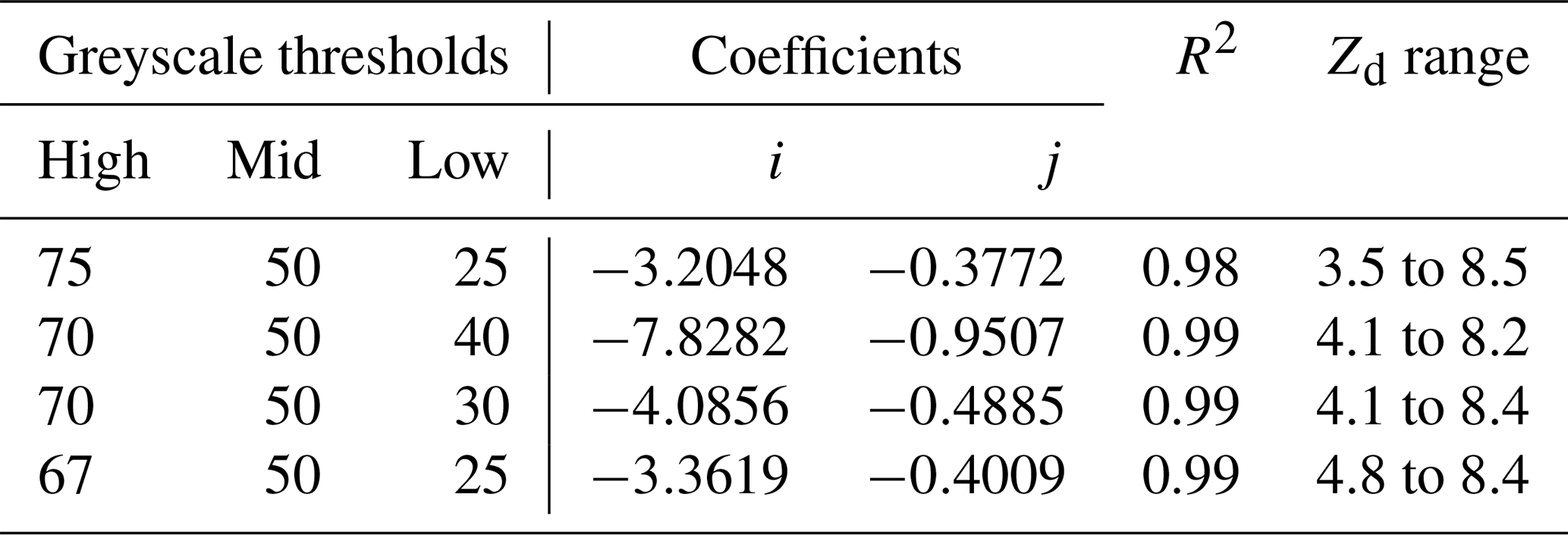

Figure 10(a) Size distributions in liquid cloud from the CIP-15 and CDP that have been averaged over a straight and level run at 14 ∘C (16:42:10 to 16:43:15, 5 September 2019). CIP-15 data have been filtered using different Zd thresholds (coloured lines). The right graph shows a subset of the full size distribution shown in the left graph. Panel (b) shows example CIP-15 images from this period. Decreases in detector intensity of 25 % to 50 %, 50 % to 75 % and > 75 % are shown as light blue, black and orange pixels, respectively.

Figure 11(a) Size distributions for a straight and level run at −42 ∘C in cirrus (16:02:00 to 16:10:00, 7 February) from a holographic imaging probe (pink markers) and the CIP-15 using different Zd thresholds. Panel (b) shows example CIP-15 images from this period. Decreases in detector intensity of 25 % to 50 %, 50 % to 75 % and > 75 % are shown as light blue, black and orange pixels, respectively. Vertical lines show the Poisson counting uncertainty, which are very small for most of the size spectrum apart from > 700 µm, where they become visible.
3.3 Sample volume
The previous section described how Zd can be determined for images as they begin to fragment. This allows a threshold Zd to be employed to remove these images from further analysis. To correctly determine the particle concentration, the sample volume needs to be adjusted to take account of the Zd threshold. The revised depth of field is calculated by setting c in Eq. (1) equal to the chosen Zd threshold. For Zd to be correctly calculated using Eq. (4) and the K07 size correction to be applicable, the entire particle needs to be imaged. Images that have pixels greater than the low greyscale threshold in contact with the edge of the optical array should not be used to calculate the concentration. The probe sample volume (SVol) for a given D0 can then be calculated using
where DLow is the image diameter using all pixels greater than the low greyscale threshold, TAS is the true airspeed, N is the number of array elements, and R is the resolution of the probe. This equation has been modified from Korolev et al. (1991) so that it uses DLow rather than D50. Across much of the probe's size range, the D25 sample area is less than 10 % smaller than the D50 sample area; however this increases for larger particles. The integration of the effective array width (NR−DLow(Z)) is performed over whichever is smaller out of the depth of field or the probe arm width.
3.4 Airborne measurements
The following section applies the results from Sect. 3.1 to 3.3 to field measurements from two research flights.
3.4.1 Liquid cloud
As part of the CLouds and Aerosol Radiative Impacts and Forcing (CLARIFY) project the FAAM Bae-146 research aircraft performed sorties out of Ascension Island. On 5 September 2017, pockets of open cells were sampled. This flight was characterised by a clean marine boundary layer and large cloud droplets/drizzle. Figure 10a shows size distributions from the CIP-15 that have been averaged over a straight and level run at 14 ∘C (16:42:10 to 16:43:15 GMT). Pink markers show the CDP size distribution averaged over the same period. The other coloured lines have been calculated using K07 using various Zd thresholds. The CDP size spectrum was relatively noisy during this period. This may be due to the very low droplet concentration (CDP total concentration = 1 cm−3) and that a significant proportion of the droplet spectrum was larger than the CDP size range. Figure 10b shows example CIP-15 images from this period. The particle diameters in this section have been calculated as the mean of the particle size along the axis of the optical array and the particle trajectory. Using a Zd threshold less than 7 significantly reduces the concentration of drops smaller than 60 µm, which is in better agreement with the CDP. The decrease is over an order of magnitude for the smallest CIP-15 bin.
3.4.2 Cirrus
A number of studies have found a persistent small ice mode in their OAP measurements of cirrus clouds (Cotton et al., 2013; Jackson et al., 2015; O'Shea et al. 2016). O'Shea et al. (2016) hypothesised that in their measurements this was largely due to out-of-focus larger crystals. Due to the size dependence of the sample volume only a relatively small proportion of mis-sized large particles are needed to cause a significant number concentration of small particles. The relationships between greyscale ratios and Zd determined in this paper have been developed using spherical droplets. Similarly, K07 is strictly only applicable to spherical droplets. However, ice crystals can be a variety of complex shapes.
To examine whether the greyscale relationships in this paper can be applied to glaciated clouds we use measurements from the PICASSO project (Parameterizing Ice Clouds using Airborne obServationS and triple-frequency dOppler radar). On 7 February 2018, the FAAM BAe-146 sampled cirrus over the south of the UK. Figure 11a shows size distributions for a straight and level run at −42 ∘C (16:02:00 to 16:10:00 GMT). Crystals were predominantly rosettes and columns, with a smaller proportion of aggregates. Example CIP-15 images from this period are shown in Fig. 11b. Particles associated with inlet shattering were minimised by filtering particles with inter-arrival times of less than s (Field et al., 2006). The particles in Fig. 11a have not been corrected using K07.
Similar to O'Shea et al. (2016), if no Zd filter is applied the CIP-15 cirrus size distribution is bimodal, with one mode at approximately 200 µm and another at the smallest measured sizes. As a more restrictive Zd threshold is applied, the small particle mode (less than 100 µm) decreases. Similar to the liquid case (Sect. 3.4.1) the concentration of small particles decreases by an order of magnitude for Zd<6 compared to when no filtering is applied. However, this algorithm does not completely remove the small particle mode. There are a number of possible explanations for this: first, the mode may be real and due to ice nucleation. However, coincident holographic measurements do not show the small particle mode (pink markers, Fig. 11a), suggesting it is an artefact associated with the OAP measurement technique. Second, it may be due to particles shattering on the inlet of the probe. However as mentioned previously, shattering events should be associated with short inter-arrival times and a stringent inter-arrival threshold has been applied to this dataset. Third, noise in the CIP-15 images will degrade the accuracy of the Zd retrieval. Finally, the non-spherical shape of ice crystals will mean that the greyscale relationships are not directly applicable. Further work is needed to examine greyscale Zd relationships for specific particle habits and whether a spherical approximation is applicable.
At large sizes the sample volume decreases with size till it is zero for particles larger than 960 µm. The Poisson counting uncertainty in the size distribution is shown as error bars in Fig. 11. As shown in Fig. 11 the number of counts becomes small and the counting uncertainty increases significantly for particles larger than approximately 700 µm.
This paper has described tests on a greyscale OAP using a droplet generator, the results of which have been compared to synthetic data. Despite recent advances in holographic instruments for cloud microphysical measurements (Fugal and Shaw, 2009) work is still needed to better characterise the uncertainties associated with this technique. Additionally holographic probes require high-performance computers to post-process the significant amounts of data they generate (e.g. HALOHolo generated several terabytes per 2–5 h flight during PICASSO). This makes it challenging to routinely deploy such instruments. Therefore, it is likely that OAPs will still be widely used in the foreseeable future. We make the following recommendations for their use:
-
K07 should be used to correct the image size of spherical particles. This algorithm is found to perform better than RB98 across much of the depth of field (Zd<6). However, K07 is not able to correct the size of the severely fragmented images of particles near the edge of the probe's depth of field (Zd>6).
-
Fragmented images from particles near the edge of the depth of field need to be removed to avoid significant bias to the derived particle size distributions, which is particularly a problem for diameters less than approximately 100 µm due to the relatively small depth of field at these sizes.
-
Greyscale information should be used to filter fragmented images and the probe's sample volume should be adjusted. The following four combinations of greyscale thresholds were tested: 25 %, 50 % and 75 %; 40 %, 50 % and 70 %; 30 %, 50 % and 70 %; and 25 %, 50 % and 67 %. Using these thresholds and the relationships presented in this paper it is possible to determine a particle's position near the edge of the depth of field. This methodology was tested on measurements from two research flights. In both cases this reduced the concentration of small particles (<60 µm) by approximately an order of magnitude, significantly improving agreement with a Mie-scattering spectrometer for the liquid case and with a holographic imaging probe for the cirrus case.
-
The data from monoscale OAPs are unreliable and should not be used for diameters below approximately 100 µm due to fragmented larger particles. A small number of monoscale probes exist that reject particles that do not have at least one detector with a > 67 % decrease in intensity. If this filtering is performed it would greatly minimise the impact of out-of-focus particles. However, this feature is not available on commonly used modern probes such as the 2DS (SPEC Inc., Lawson et al., 2006).
-
Reintroducing a 67 % intensity rejection criteria on monoscale probes should be high priority if possible. If this requires hardware modifications, it may be more appropriate to upgrade to full greyscale capability.
-
Past datasets from greyscale OAPs should be re-examined. The filtering and sample volume adjustments presented in this paper should be applied.
The data presented here can be provided on request to the contact author.
SJO, JC and JD performed laboratory experiments. SJO, JC, JD, RC, WS and IC collected and processed airborne measurements. AB performed model experiments. SB provided and supported the use of the holographic probe. SJO and JC analysed and interpreted the data. SJO wrote the paper. All authors commented on and/or edited the paper.
The authors declare that they have no conflict of interest.
The authors would like to thank Brian Derby, Andy Wallwork and Rachel Saunders for their assistance with the drop generator setup. We would like to thank Chris Westbrook and the PICASSO and CLARIFY teams for provision of the airborne data. Airborne data were obtained using the BAe-146-301 Atmospheric Research Aircraft (ARA) flown by Directflight Ltd and managed by the Facility for Airborne Atmospheric Measurements (FAAM), which is a joint entity of the Natural Environment Research Council (NERC) and the Met Office. The CIP-15s were provided by the National Centre for Atmospheric Science and FAAM. The National Centre for Atmospheric Science provided support for the droplet generator experiments.
This research has been supported by the Natural Environment Research Council (grant no. NE/P012426/1 and NE/L013584/1).
This paper was edited by Andrew Sayer and reviewed by Darrel Baumgardner, Jeff French, and David Delene.
Baumgardner, D. and Korolev, A.: Airspeed Corrections for Optical Array Probe Sample Volumes, J. Atmos. Ocean. Tech., 14, 1224–1229, https://doi.org/10.1175/1520-0426(1997)014<1224:ACFOAP>2.0.CO;2, 1997.
Baumgardner, D., Jonsson, H., Dawson, W., O'Connor, D., and Newton, R.: The cloud, aerosol and precipitation spectrometer: a new instrument for cloud investigations, Atmos. Res., 59–60, 251–264, https://doi.org/10.1016/S0169-8095(01)00119-3, 2001.
Cotton, R. J., Field, P. R., Ulanowski, Z., Kaye, P. H., Hirst, E., Greenaway, R. S., Crawford, I., Crosier, J., and Dorsey, J.: The effective density of small ice particles obtained from in situ aircraft observations of mid-latitude cirrus, Q. J. Roy. Meteor. Soc., 139, 1923–1934, 2013.
Field, P. R.: Aircraft Observations of Ice Crystal Evolution in an Altostratus Cloud, J. Atmos. Sci., 56, 1925–1941, https://doi.org/10.1175/1520-0469(1999)056<1925:AOOICE>2.0.CO;2, 1999.
Field, P. R., Heymsfield, A. J., and Bansemer, A.: Shattering and Particle Interarrival Times Measured by Optical Array Probes in Ice Clouds, J. Atmos. Ocean. Tech., 23, 1357–1371, 2006.
Fox, S., Mendrok, J., Eriksson, P., Ekelund, R., O'Shea, S. J., Bower, K. N., Baran, A. J., Harlow, R. C., and Pickering, J. C.: Airborne validation of radiative transfer modelling of ice clouds at millimetre and sub-millimetre wavelengths, Atmos. Meas. Tech., 12, 1599–1617, https://doi.org/10.5194/amt-12-1599-2019, 2019.
Fugal, J. P. and Shaw, R. A.: Cloud particle size distributions measured with an airborne digital in-line holographic instrument, Atmos. Meas. Tech., 2, 259–271, https://doi.org/10.5194/amt-2-259-2009, 2009.
Gurganus, C. and Lawson, P.: Laboratory and flight tests of 2D imaging probes: Toward a better understanding of instrument performance and the impact on archived data, J. Atmos. Ocean. Tech., 35, 7, 1533–1553, https://doi.org/10.1175/JTECH-D-17-0202.1, 2018.
Jackson, R. C., McFarquhar, G. M., Fridlind, A. M., and Atlas, R.: The dependence of cirrus gamma size distributions expressed as volumes in N0-λ-μ phase space and bulk cloud properties on environmental conditions: Results from the Small Ice Particles in Cirrus Experiment (SPARTICUS), J. Geophys. Res.-Atmos., 120, 10351–10377, https://doi.org/10.1002/2015JD023492, 2015.
Jang, D., Kim, D., and Moon, J.: Influence of fluid physical properties on ink-jet printability, Langmuir, 25, 2629–2635, 2009.
Joe, P. and List, R.: Testing and performance of two dimensional optical array spectrometers with greyscale, J. Atmos. Ocean. Tech., 4, 139–150, 1987.
Knollenberg, R. G.: The optical array: An alternative to scattering or extinction for airborne particle size determination, J. Appl. Meteorol., 9, 86–103, https://doi.org/10.1175/1520-0450(1970)009<0086:TOAAAT>2.0.CO;2, 1970.
Korolev, A.: Reconstruction of the sizes of spherical particles from their shadow images, Part I: Theoretical considerations, J. Atmos. Ocean. Tech., 24, 376–389, 2007.
Korolev, A. V., Kuznetsov, S. V., Makarov, Y. E., and Novikov, V. S.: Evaluation of measurements of particle size and sample area from optical array probes, J. Atmos. Ocean. Tech., 8, 514–522, 1991.
Lance, S., Brock, C. A., Rogers, D., and Gordon, J. A.: Water droplet calibration of the Cloud Droplet Probe (CDP) and in-flight performance in liquid, ice and mixed-phase clouds during ARCPAC, Atmos. Meas. Tech., 3, 1683–1706, https://doi.org/10.5194/amt-3-1683-2010, 2010.
Lawson, R. P., O'Connor, D., Zmarzly, P., Weaver, K., Baker, B., Mo, Q., and Jonsson, H.: The 2D-S (stereo) probe: Design and preliminary tests of a new airborne, high-speed, high-resolution particle imaging probe, J. Atmos. Ocean. Tech., 23, 1462–1477, https://doi.org/10.1175/JTECH1927.1, 2006.
Lawson, R. P., Woods, S., and Morrison, H.: The Microphysics of Ice and Precipitation Development in Tropical Cumulus Clouds, J. Atmos. Sci., 72, 2429–2445, https://doi.org/10.1175/JAS-D-14-0274.1, 2015.
Liu, Y.: Inkjet printed drops and three-dimensional ceramix structures, PhD Thesis, University of Manchester, 2016.
Mace, G. G. and Benson, S.: Diagnosing cloud microphysical process information from remote sensing measurements: A feasibility study using aircraft data, Part I: Tropical anvils measured during TC4, J. Appl. Meteor. Climatol., 56, 633–649, https://doi.org/10.1175/JAMC-D-16-0083.1, 2017.
O'Shea, S. J., Choularton, T. W., Lloyd, G., Crosier, J., Bower, K. N., Gallagher, M., Abel, S. J., Cotton, R. J., Brown, P. R. A., Fugal, J. P., Schlenczek, O., Borrmann, S., and Pickering, J. C.: Airborne observations of the microphysical structure of two contrasting cirrus clouds, J. Geophys. Res., 121, 13510–13536, https://doi.org/10.1002/2016JD025278, 2016.
Reuter, A. and Bakan, S.: Improvements of cloud particle sizing with a 2-D-grey probe, J. Atmos. Ocean. Tech., 15, 1196–1203, 1998.
Schlenczek, O.: Airborne and ground-based holographic measurement of hydrometeors in liquid-phase, mixed-phase and ice clouds, PhD Thesis, University of Mainz, 2017.
Wendisch, M. and Brenguier, J.-L. (Eds.): Airborne Measurements for Environmental Research: Methods and Instruments, vol. ISBN: 978-3-527-40996-9, Wiley-VCH Verlag GmbH and Co. KGaA, Weinheim, Germany, 2013.