Automated compact mobile Raman lidar for water vapor measurement: instrument description and validation by comparison with radiosonde, GNSS, and high-resolution objective analysis

We developed an automated compact mobile Raman lidar (MRL) system for measuring the vertical distribution of the water vapor mixing ratio (w) in the lower troposphere, which has an affordable cost and is easy to operate. The MRL was installed in a small trailer for easy deployment and can start measurement in a few hours, and it is capable of unattended operation for several months. We describe the MRL system and present validation results obtained by comparing the MRL-measured data with collocated radiosonde, Global Navigation Satellite System (GNSS), and high-resolution objective analysis data. The comparison results showed that MRL-derived w agreed within 10 % (root-mean-square difference of 1.05 g kg⁻¹) with values obtained by radiosonde at altitude ranges between 0.14 and 1.5 km in the daytime and between 0.14 and 5–6 km at night in the absence of low clouds; the vertical resolution of the MRL measurements was 75–150 m, their temporal resolution was less than 20 min, and the measurement uncertainty was less than 30 %. MRL-derived precipitable water vapor values were similar to or slightly lower than those obtained by GNSS at night, when the maximum height of MRL measurements exceeded 5 km. The MRL-derived w values were at most 1 g kg⁻¹ (25 %) larger than local analysis data. A total of 4 months of continuous operation of the MRL system demonstrated its utility for monitoring water vapor distributions in the lower troposphere.

1 Introduction

In recent years, the occurrence frequency of localized heavy rainfall capable of causing extensive damage has been increasing in urban areas of Japan (Japan Meteorological Agency (JMA), 2017). For early prediction of heavy rainfall, a numerical weather prediction (NWP) model is employed along with conventional meteorological observation data. However, the lead time (period of time between the issuance of a forecast and the occurrence of the rainfall) and accuracy of the prediction are limited, in part, because of the coarse temporal and spatial resolutions of water vapor distribution observations. To improve those observations, we developed a low-cost automated mobile Raman lidar (MRL) system that can continuously measure the vertical distribution of water vapor in the lower troposphere. The MRL can be easily deployed at a site upwind of a potential heavy rainfall area and start measurement in a few hours to monitor the vertical water vapor distribution before a rainfall event. As several studies have already demonstrated a strong and positive impact of the water vapor lidar data on the initial water vapor field of the numerical weather prediction mesoscale model by using the three- or four-dimensional variational method (Wulfmeyer et al., 2006; Grzeschik et al., 2008; Bielli et al., 2012), the MRL-measured data can be assimilated into a nonhydrostatic mesoscale model (NHM) (Saito et al., 2007) by the local ensemble transform Kalman filter (LETKF) method (Kunii, 2014) to improve the initial condition of the water vapor field and consequently the rainfall forecast. Given the temporal and vertical resolutions of the model and the assimilation window length, the required measurement resolutions are at most 30 min in time and 200 m in the vertical direction. The measurement altitude range should be at least between 0.2 and 2 km because Kato (2018) has reported that the equivalent potential temperature at a height of 500 m, which is a function of the water vapor concentration at that height, is an important parameter for forecasting heavy rainfall in the Japanese area because the inflow of moist air, which can cause heavy rain, mainly occurs at around that altitude. Wulfmeyer et al. (2015) discussed the requirements of accuracy of the lower-tropospheric water vapor measurement for data assimilation and reported that it should be smaller than 10 % in noise error and <5 % in bias error. In addition to the requirement of measurement accuracy, reducing the cost of the lidar is important because it makes it easier to distribute them around the forecasting area to increase the opportunity of detecting the inflow. We developed our MRL system to meet these requirements as much as possible within the total material cost of ∼ USD 250 000. The Raman lidar technique is a well-established technique for measuring the water vapor distribution in the troposphere (e.g., Melfi et al., 1969; Whiteman et al., 1992), and the systems have been in operation for decades at stations around the world (Turner et al., 2016; Dinoev et al., 2013; Reichardt et al., 2012; Leblanc et al., 2012). Field-deployable systems have also been developed by several institutes (Whiteman et al., 2012; Chazette et al., 2014; Engelmann et al., 2016). Our MRL system is a compact mobile system that can be deployed on a standard vehicle and operated unattended for several months by remote control. As the first step of our goal aiming to develop the heavy rainfall forecasting system, here we describe our mobile lidar system and present validation results obtained by comparing the MRL-measured data with data obtained by other humidity sensors as well as objective analysis data. Section 2 of this paper describes the MRL instrumentation and the data analysis method. Section 3 presents the validation results obtained by comparing the MRL measurements with collocated radiosonde measurements, GNSS data, and high-resolution objective analysis data provided by the JMA. Section 4 is a summary.

2 Instrumentation

2.1 Transmitter and receiver optics

The MRL system employs a Nd:YAG laser (Continuum Surelite EX) operating at 355 nm with a pulse energy of 200 mJ and a repetition rate of 10 Hz. The beam diameter is expanded fivefold to a diameter of ∼5 cm by a beam expander (CVI, USA), and the beam is emitted vertically into the atmosphere. The light backscattered by atmospheric gases and particles is collected by a custom-made Cassegrain telescope (primary mirror diameter of 0.35 m, focal length 3.1 m; Kyoei Co., Japan). The focal point of the telescope is within the tube to shorten the length of the receiving system. Light baffles placed inside the telescope tube prevent stray light from entering the detectors. The received light is separated into three spectral components, Raman water vapor (407.5 nm), nitrogen (386.7 nm), and elastic (355 nm) backscatter light, with dichroic beam splitters and interference filters (IFs) (Barr Materion, USA), shortcut filters (Isuzu Glass ITY385, Japan), and short-pass filters (SHPF-50S-440, Sigmakoki, Japan), and is detected by photomultiplier tubes (PMTs) (R8619, Hamamatsu, Japan). The interference filter angles of the Raman channels are tuned manually to maximize the transmission of the Raman backscatter signal. To avoid signal saturation of the PMTs, we inserted neutral density filters before the PMTs. The signals are acquired with a transient recorder (Licel TR-20-160) operating in analog (12 bit) and photon-counting (20 MHz) modes. The data are stored on the hard disk of a personal computer (PC). The MRL can be operated remotely by issuing commands (e.g., turn high voltage of PMTs on or off, start or stop lasing, start or stop data acquisition, and transfer data) to the PC via wireless Internet communication (Table 1, Fig. 1).

Table 1 Specifications of the mobile Raman lidar.

Figure 1 Schematic diagram of the mobile Raman lidar system.

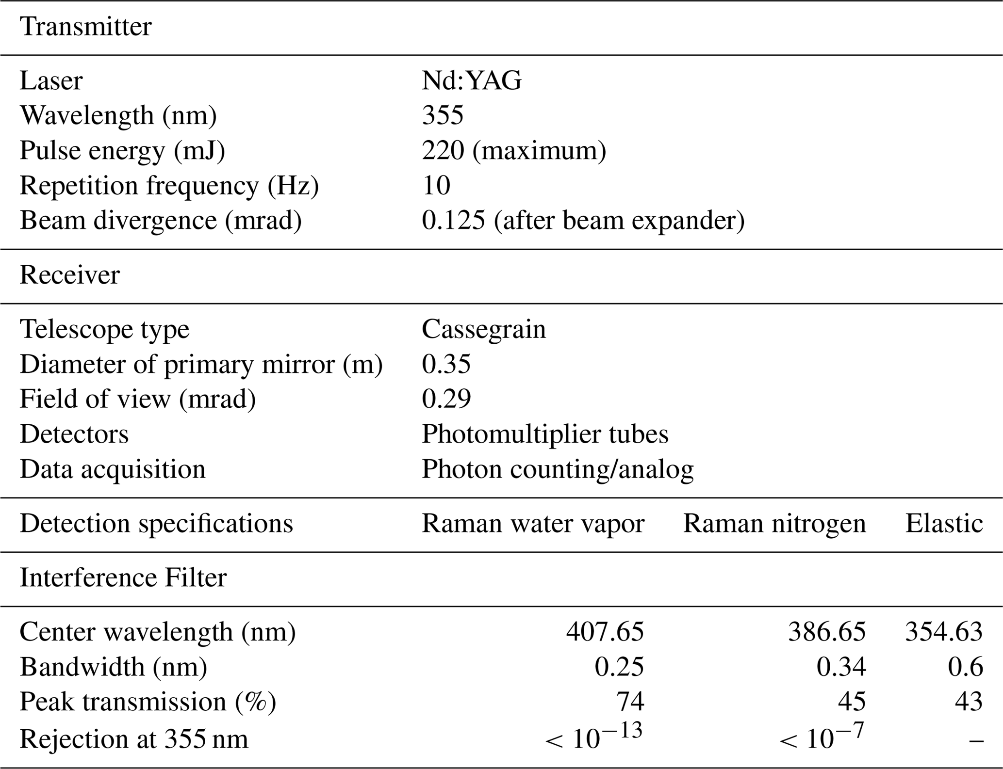
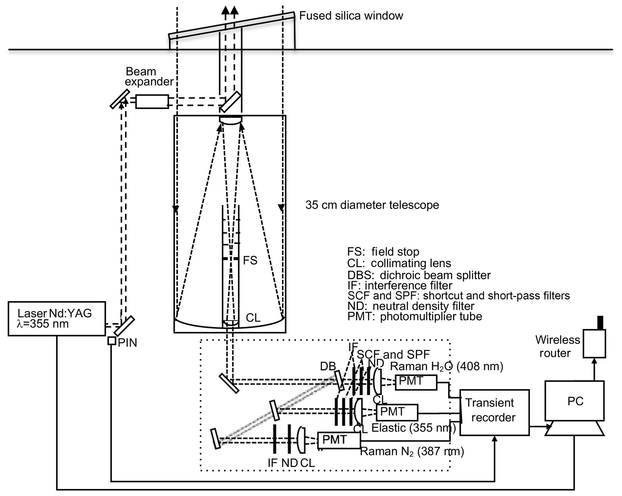
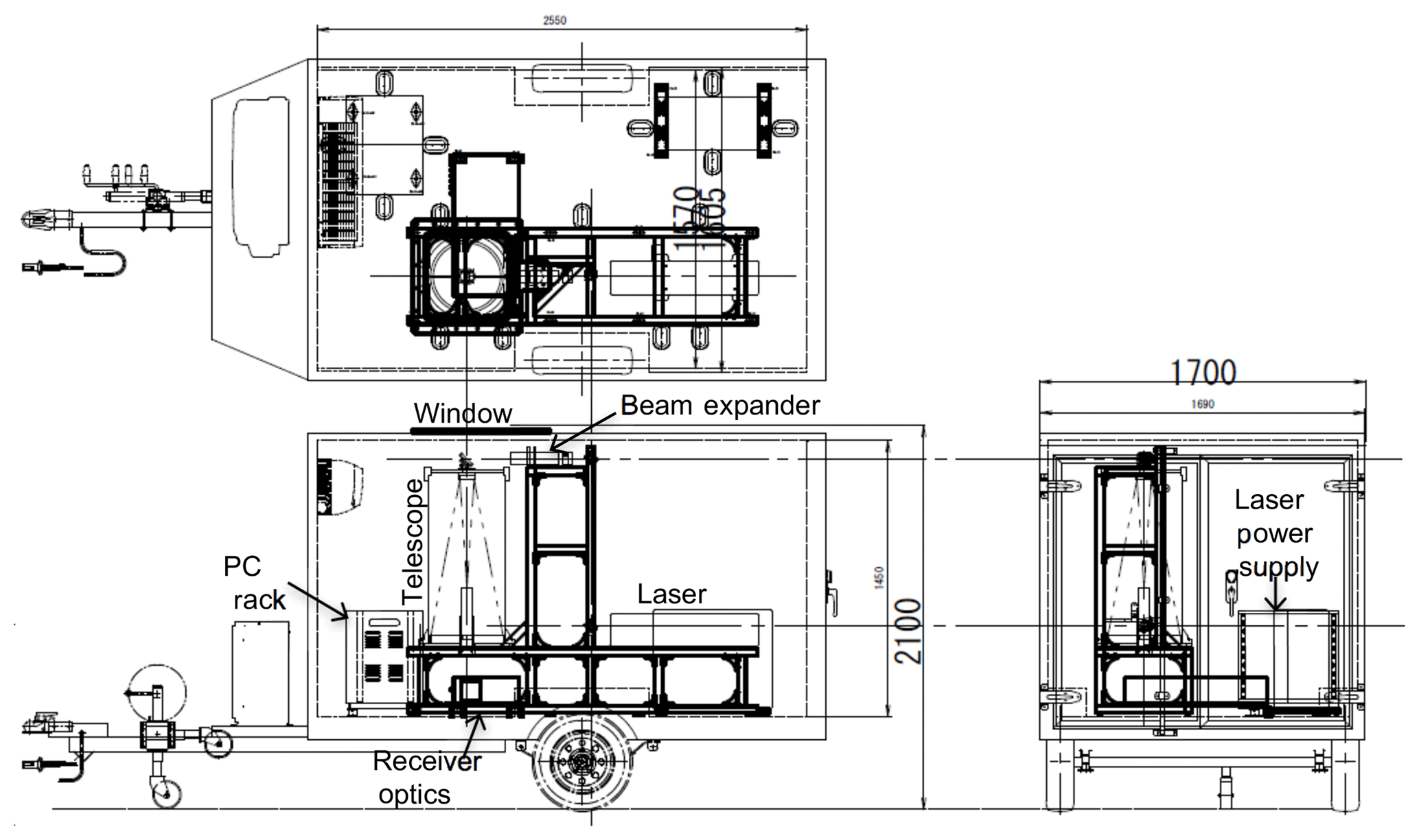
Figure 2 Layout of the mobile Raman lidar system in its trailer. Dimensions are in millimeters.

Figure 3 Photographs of the MRL trailer (a) and its interior (b).

2.2 Trailer

The MRL system is enclosed in a container with outside dimensions of 1.7 m by 4.2 m by 2.1 m high (Figs. 2 and 3). The total weight, including the lidar system and the trailer, is approximately 800 kg. The trailer can be towed behind any standard-sized vehicle; therefore, anyone who holds a basic-class driver's license can tow it in Japan. The temperature inside the trailer was maintained within a range of ±2 ^∘C between 22 and 32 ^∘C by an air conditioner during the experimental period in 2016. We did not find any change of the optical alignment of the transmitter and receiver with the change of the temperature. A fused silica window ($\mathrm{47}\mathrm{cm}\times \mathrm{42}\mathrm{cm}\times \mathrm{1}\mathrm{cm}$ thick, Kiyohara Optics, Inc.) with an antireflection coating installed at a tilt angle of 10^∘ above the receiving telescope enables the MRL to be operated regardless of the weather. To prevent direct sunlight from entering the telescope, a chimney-type light baffle with a height of 2 m is mounted on top of the trailer. The system requires a single-phase, three-wire-type 100/200 V power supply with a maximum current of 10 A (5–7 A during normal operation).

2.3 Data analysis

The water vapor mixing ratio (w) is obtained from the observed Raman backscatter signal of water vapor and nitrogen as follows:

$$w\left(z\right)=K{\displaystyle \frac{O_{{\mathrm{H}}_{\mathrm{2}}\mathrm{O}}\left(z\right)}{O_{{\mathrm{N}}_{\mathrm{2}}}\left(z\right)}}{\displaystyle \frac{P_{{\mathrm{H}}_{\mathrm{2}}\mathrm{O}}\left(z\right)}{P_{{\mathrm{N}}_{\mathrm{2}}}\left(z\right)}}\mathrm{\Delta }T\left(z_{\mathrm{0}}z\right),$$

with

$$\begin{array}{}\text{(1)}& \mathrm{\Delta }T={\displaystyle \frac{e^{{\int }_{z_{\mathrm{0}}}^z[{\mathit{\alpha }}_{{\mathrm{H}}_{\mathrm{2}}\mathrm{O}}^{\mathrm{m}}\left(z{}^{\prime }\right)+{\mathit{\alpha }}_{{\mathrm{H}}_{\mathrm{2}}\mathrm{O}}^{\mathrm{p}}\left(z{}^{\prime }\right)]\mathrm{d}z{}^{\prime }}}{e^{{\int }_{z_{\mathrm{0}}}^z[{\mathit{\alpha }}_{N_{\mathrm{2}}}^{\mathrm{m}}\left(z{}^{\prime }\right)+{\mathit{\alpha }}_{{\mathrm{N}}_{\mathrm{2}}}^{\mathrm{p}}\left(z{}^{\prime }\right)]\mathrm{d}z{}^{\prime }}}},\end{array}$$

where K is the calibration coefficient of the water vapor mixing ratio, O_X (z) is the beam overlap function of the receiver's channel, P_X (z) is the noise-subtracted Raman backscatter signal of molecular species X (H₂O or N₂) at height z from the lidar at z₀, ΔT is the transmission ratio of the Raman signals between the lidar at z₀ and z, and ${\mathit{\alpha }}_X^{\mathrm{m}}$ and ${\mathit{\alpha }}_X^{\mathrm{p}}$ are the molecular and particle extinction coefficients of X at the wavelength of the Raman scattering. The P_X (z) for each receiving channel was obtained by connecting the photon counting and analog data using a count rate range of 1–10 MHz (mostly 0.2–0.4 km for the water vapor and 0.5–0.9 km for the nitrogen channels) to gain a high dynamic range. The value of K was obtained by comparing the uncalibrated MRL-derived value of w (i.e., w computed assuming K=1 in Eq. 1) with w obtained with a radiosonde launched 80 m northeast of the MRL at 20:30 LST by a weighted least-squares method (Sakai et al., 2007) between altitudes of 1 and 5 km and taking the average over the measurement period. See Sect. 2.4 for the values of K obtained in this manner and their temporal variation. In this system, the ratio of the beam overlap functions ($\frac{O_{{\mathrm{H}}_{\mathrm{2}}\mathrm{O}}\left(z\right)}{O_{{\mathrm{N}}_{\mathrm{2}}}\left(z\right)})$ is 1 above an altitude of 0.5 km, and below that altitude it deviates slightly from 1; these values were determined by comparing the MRL-derived value of w without overlap correction (i.e., w obtained by assuming $\frac{O_{{\mathrm{H}}_{\mathrm{2}}\mathrm{O}}\left(z\right)}{O_{{\mathrm{N}}_{\mathrm{2}}}\left(z\right)}=\mathrm{1}$ in Eq. 1) with w obtained by radiosonde measurements (see Sect. 2.5). To determine ΔT, we calculated ${\mathit{\alpha }}_X^{\mathrm{m}}$ using molecular extinction cross section (Bucholz, 1995) atmospheric density obtained from the radiosonde measurement made closest to the MRL measurement period; we did not take the differential aerosol extinction for the two Raman wavelengths into account because it is usually less than 5 % below the altitude of 7 km (i.e., ΔT ranges from 1 to 0.95 from the lidar position to 7 km) under normal aerosol loading conditions (Whiteman et al., 1992). The temporal and vertical resolutions of the raw data were 1 min and 7.5 m, respectively. To reduce the statistical uncertainty of the derived w, we averaged the raw data over 20 min and reduced the vertical resolution to 75 m below 1 km in altitude and 150 m above that. The measurement uncertainty of w was estimated from the photon counts by assuming Poisson statistics (e.g., Whiteman, 2003) and the uncertainty of the calibration coefficient as follows:

$$\mathit{\delta }w\left(z\right)={\left[{\left({\displaystyle \frac{\mathit{\delta }K}{K}}\right)}^{\mathrm{2}}+{\left({\displaystyle \frac{\mathit{\delta }{P}_{{\mathrm{H}}_{\mathrm{2}}\mathrm{O}}\left(z\right)}{P_{{\mathrm{H}}_{\mathrm{2}}\mathrm{O}}\left(z\right)}}\right)}^{\mathrm{2}}+{\left({\displaystyle \frac{\mathit{\delta }{P}_{{\mathrm{N}}_{\mathrm{2}}}\left(z\right)}{P_{{\mathrm{N}}_{\mathrm{2}}}\left(z\right)}}\right)}^{\mathrm{2}}\right]}^{\frac{\mathrm{1}}{\mathrm{2}}},$$

where

$$\begin{array}{}\text{(2)}& \mathit{\delta }{P}_X={\left(P_{X,\mathrm{signal}}+\mathrm{2}{P}_{X,\mathrm{noise}}\right)}^{\frac{\mathrm{1}}{\mathrm{2}}}.\end{array}$$

The signal (P_X, signal) was obtained from the total backscatter signal by subtracting the background noise (P_X, noise), which was computed by taking the average of the total signal between the altitudes of 80 and 120 km, where atmospheric backscattering was expected to be negligible. The uncertainty of the calibration coefficient (δK) was estimated as the standard deviation of K, which was obtained from the comparison of uncalibrated MRL-derived data with the radiosonde data for the measurement period. As quality control (QC) of the derived data, we excluded data with uncertainty larger than 30 % or w>30 g kg⁻¹.

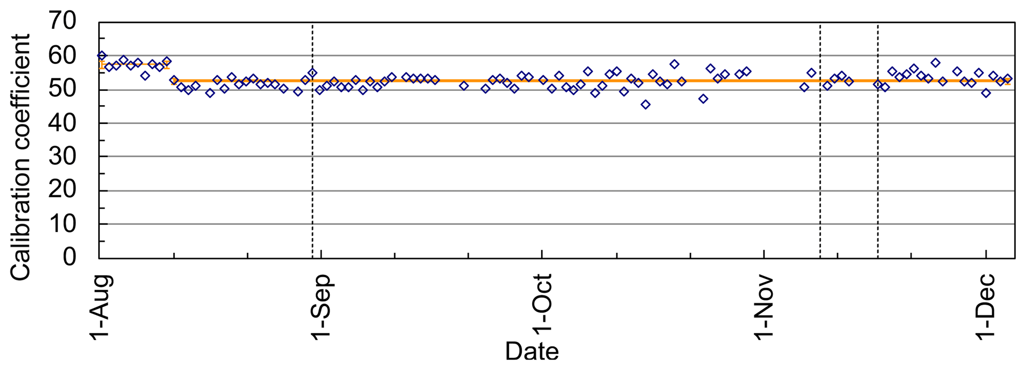
Figure 4 Temporal variation in the calibration coefficient of the water vapor mixing ratio (K) for the MRL obtained by comparison with collocated radiosonde measurements at 20:30 LST from August to December 2016. The horizontal orange lines show the averages before and after 12 August. The vertical dotted lines indicate dates on which the optical axis was adjusted.

2.4 Calibration coefficient of the water vapor mixing ratio

To obtain the absolute value of w from the lidar signals, the calibration coefficient K of Eq. (1) is necessary. To obtain the value of K, several methods have been proposed and tested; they used external reference water vapor sensor measurements (e.g., radiosonde, GNSS, microwave radiometer, or sun photometer) or external reference light sources (e.g., diffuse sunlight or a standard lamp) and the effective Raman cross sections. A comprehensive review of these methods can be found elsewhere (Dai et al., 2018; David et al., 2017). In this study, we used the most conventional and reliable method by using radiosonde as described in Sect. 2.3. However, temporal change in K is a critical problem for long-term operation of the system because if the temporal variation is large, K must be obtained frequently during the measurement period. We investigated this problem by examining the temporal variation in K values obtained by comparing uncalibrated MRL-derived w with collocated radiosonde measurements (see Sect. 3.1 for the details) obtained daily at 20:30 LST from August to December 2016 (Fig. 4). During the test period, the MRL system was operated nearly continuously at the Meteorological Research Institute in Tsukuba, except for short interruptions for flash lamp replacement (31 August and 1 November), power outages (18 August and 23 October), and trailer inspection (31 October to 6 November). We calculated K only for the nighttime (20:30 LST) data because at night the MRL measurement uncertainty was small between altitudes of 1 and 5 km (see Sect. 3.1). After 12 August, the value of K was nearly constant during the test period: $\text{mean}\pm \text{standard deviation}=\mathrm{52.4}\pm \mathrm{2.1}$ (Fig. 4). Unfortunately, the reason for the abrupt change in K on 11 August from 57.4±1.5 is unknown because we did not make any changes to the instrument at that time. Nevertheless, given the uncertainty of K (4 % in this case), we may say that the MRL can be operated for at least 4 months without calibration. The possible reason for the variation in K is the variation in temperature in the trailer that can change the sensitivity of PMTs and center wavelength of IFs. During the experimental period, the variation in temperature in the trailer was at most ±5 K, which corresponds to <6 % variation in the effective Raman backscattering cross section ratio and thus K, assuming that the temperature variation in the sensitivity of PMT is <0.4 % K⁻¹ (Hamamatsu Photonics, 2007) and that of the filter CWL is <0.0035 nm K⁻¹ (Fujitok, Japan, personal communication, 2014). To reduce the temperature variations, we need more stringent control of the temperature of the receiving system. We also examined the value of K before the system was moved from Tsukuba to the Tokyo Bay area (110 or 70 km from Tsukuba) with that obtained after the move, from 15 June to 9 November 2017 (not shown). Before the system was moved, K was 46.9±1.8, and afterward it was 43.1±2.3, a change of 8.6 % (we note also that after the telescope focus was readjusted in January 2017, the value of K changed from what it had been in 2016). These results indicate that the calibration coefficient should be determined before and after deployment of the system, and the average and standard deviation of those values should be used for K and δK.

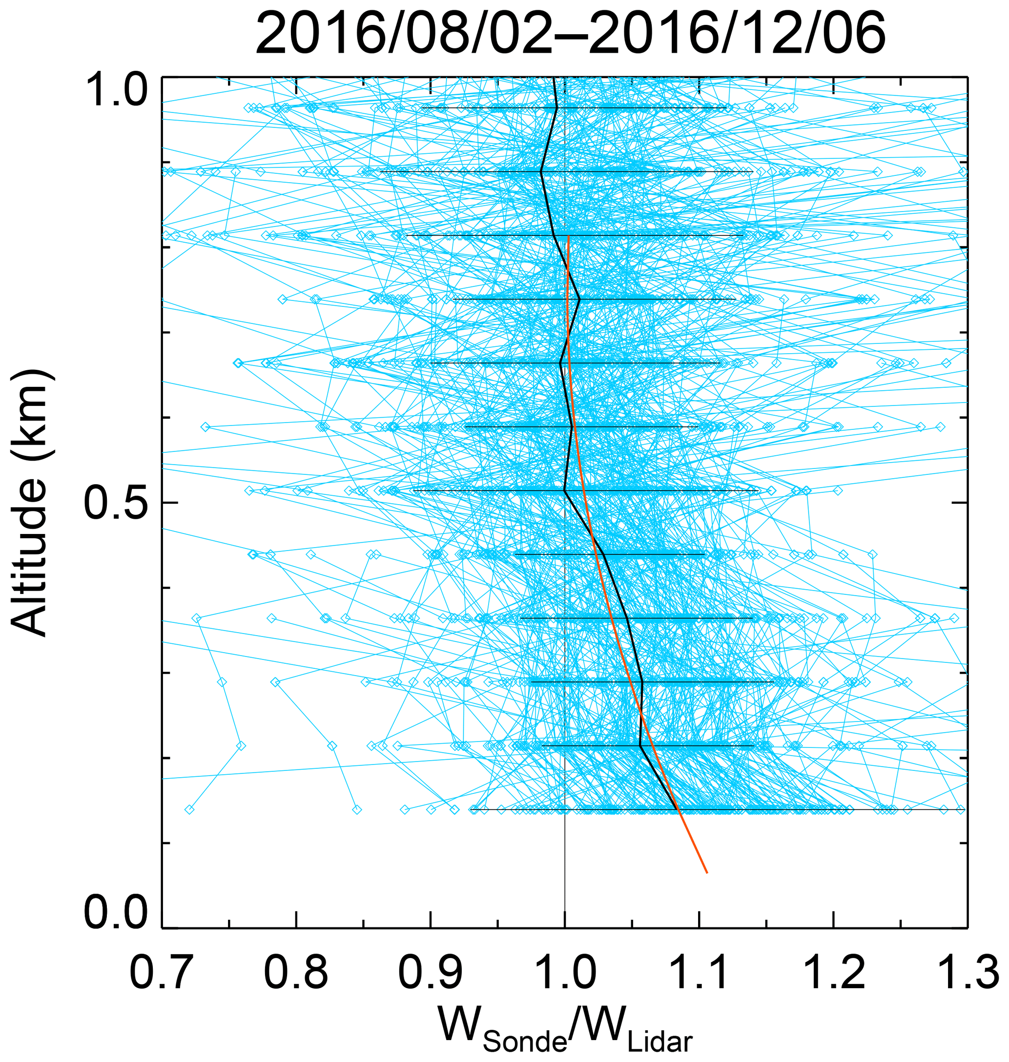
Figure 5 Vertical distribution of the ratio of w obtained by radiosonde (w_Sonde) to w obtained with the MRL system without beam overlap correction (w_Lidar) from 2 August to 6 December 2016. The individual profiles are shown by the thin blue lines with diamonds. The solid black line and the error bars are averages and standard deviations over a 75 m height interval. A quadric curve (orange line) was fitted to the averaged values.

2.5 Beam overlap correction for the Raman channels

Values of w calculated from the MRL signals for altitudes below 0.5 km were systematically lower than values obtained with the radiosonde when it was assumed that the beam overlap functions for the Raman water vapor and nitrogen channels were equal (i.e., $\frac{O_{{\mathrm{H}}_{\mathrm{2}}\mathrm{O}}\left(z\right)}{O_{{\mathrm{N}}_{\mathrm{2}}}\left(z\right)}=\mathrm{1}$). When we compared the vertical distribution of the ratio of w obtained by radiosonde to that obtained by the MRL without beam overlap correction (Fig. 5), we found considerable variation among individual profiles, but the average value of the ratio increased from 1 to 1.1 with a decrease in altitude from 0.7 to 0.1 km. Possible reasons for the difference in the overlap functions of the two Raman channels at low altitude are the difference in the optical paths (Fig. 1) and the spatial inhomogeneity of PMT sensitivity (Simeonov et al., 1999; Hamamatsu Photonics, 2007). To correct for the difference, we derived the ratio of beam overlap functions by comparing w obtained with the MRL under the assumption of $\frac{O_{{\mathrm{H}}_{\mathrm{2}}\mathrm{O}}\left(z\right)}{O_{{\mathrm{N}}_{\mathrm{2}}}\left(z\right)}=\mathrm{1}$ with w obtained by radiosonde. Then, we calculated the mean vertical profile of the ratios and fitted a quadric curve to the profile for use in Eq. (1) to calculate w. The magnitude of the correction increased from 1 % at 0.5 km altitude to 8 % at 0.1 km. The uncertainty of the correction was estimated to be 8 % from the standard deviation of the profiles. The possible reasons for the variation among the profiles are difference of the measurement period and temporal resolution (i.e., 20 min average for the lidar and approximately 1 s for the radiosonde), difference of the vertical resolution (i.e., 75 m for the lidar and 20–300 m that depends on the significant pressure level interval for the radiosonde), and lidar noise. The variation should be reduced if using the data measured above the lidar by using a kite (Totems and Chazette, 2016) or unmanned aerial vehicles.

3 Validation results

To provide error estimates for the MRL system and characterize its performance, measurements for validation of the MRL system measurements were made on 120 days, from 2 August to 6 December 2016, over Tsukuba, Japan (36.06^∘ N, 140.12^∘ E). There have been many studies for the validation of the Raman lidar systems using robust approaches (e.g., Behrendt, et al., 2007; Bhawar et al., 2011; Herold et al., 2011). We validated MRL-derived w values by comparing them with collocated and coincident radiosonde, GNSS, and high-resolution local analysis (LA) data, which are described below.

3.1 Comparison with radiosonde measurements

Radiosondes (RS-11G, Meisei Electric, Co., Japan) were launched twice daily (08:30 and 20:30 LST) from an aerological observatory located 80 m northeast of the MRL, and, according to the manufacturer, the measurement uncertainty of relative humidity by the RS-11G radiosonde is 5 % in the lower troposphere and 7 % in the upper troposphere (http://www.meisei.co.jp/english/products/RS-11G_E.pdf, last access: 14 January 2019).

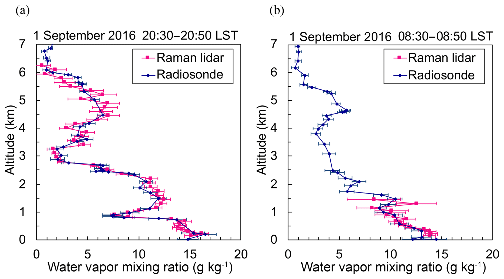
Figure 6 Vertical distributions of the water vapor mixing ratio obtained with the MRL (magenta) and radiosonde (dark blue) on 1 September 2016 over Tsukuba. The measurement periods for the MRL were (a) 08:30–08:50 and (b) 20:30–20:50 LST, and the radiosondes were launched at (a) 08:30 LST and (b) 20:30 LST. MRL data with uncertainty of less than 30 % are plotted.

3.1.1 Vertical distribution

We compared the vertical distribution of w obtained with the MRL with w obtained by radiosondes launched at 08:30 and 20:30 LST on 1 September 2016 over Tsukuba (Fig. 6). The ascent speed of the radiosondes was 5–6 m s⁻¹, so they reached a height of about 7 km after 20 min. The MRL data were accumulated over the 20 min following the radiosonde launch. The vertical resolution is reduced to 75 m below an altitude of 1 km and to 150 m above that to increase the signal-to-noise ratio (SNR) of the Raman backscatter signals. The values of w obtained with the MRL agreed well for the altitude range of 0.14–1.7 km with w obtained by radiosonde during 08:30–08:50 LST (Fig. 6a), and they agreed well for altitudes up to 6.2 km with radiosonde measurements made during 20:30–20:50 LST (Fig. 6b). Mean differences were 0.8 g kg⁻¹ (7 %) for the 08:30 LST radiosonde launch and 0.7 g kg⁻¹ (15 %) for the 20:30 LST launch. The maximum height of MRL measurements with an uncertainty of less than 30 % was only 1.5 km in the daytime because solar light reduces the SNR of the Raman backscatter signals; for example, at 08:30 LST on 1 September 2016, the solar zenith angle was 50^∘ (Fig. 6a).

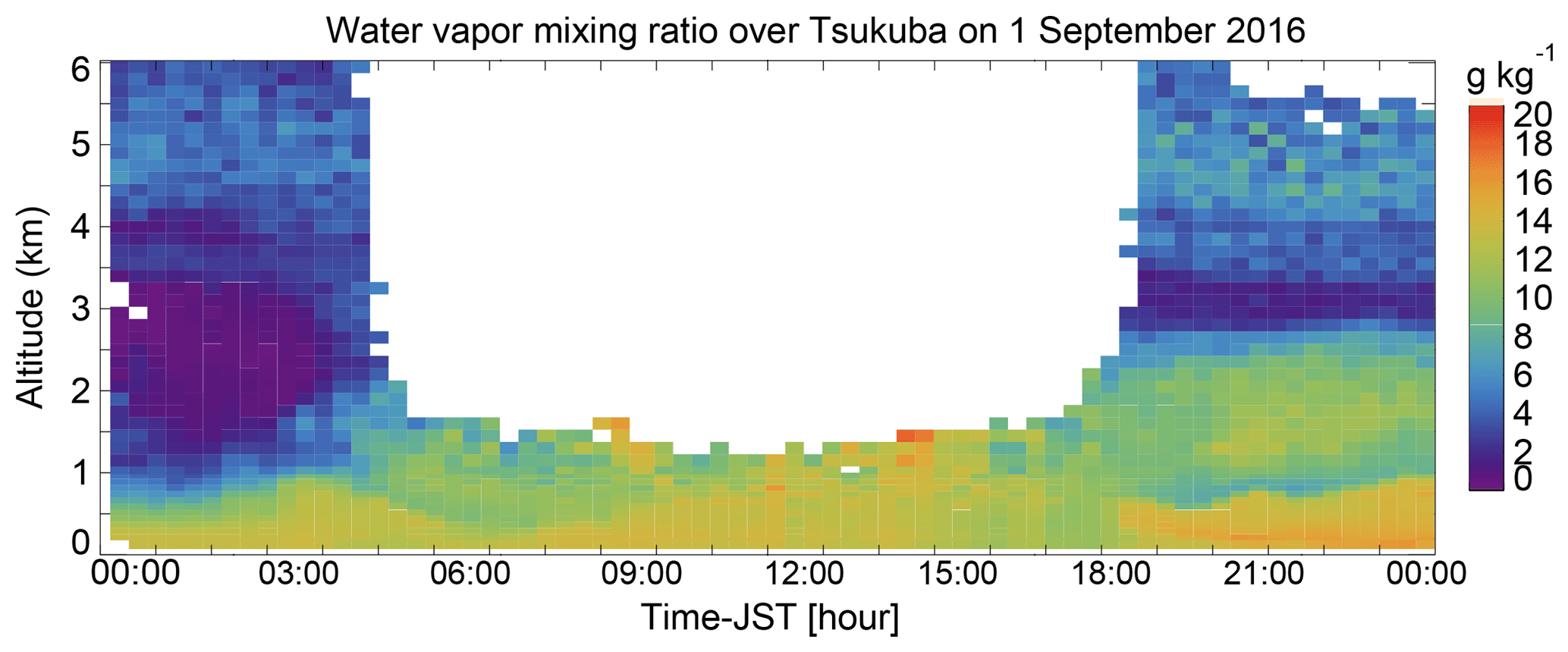
Figure 7 Altitude–time cross section of water vapor mixing ratios obtained with the MRL on 1 September 2016. Data with uncertainty of less than 30 % are plotted. Arrows at the bottom show the start of the measurement periods for the data shown in Fig. 6.

The altitude–time cross section of w obtained with the MRL on 1 September 2016 (Fig. 7) showed considerable diurnal moisture variation below an altitude of 3 km. The top height of a moist region (w>12 g kg⁻¹) present below an altitude of 1 km during 00:00–03:00 LST increased to above 2 km as the sun rose during 03:00–06:00 LST. At midday, the top height of the moist region was probably above 1.5 km (although it cannot be seen because of the low SNR in strong sunlight). After sunset, it remained at an altitude of 2.5 km, which probably corresponded to the top of a residual layer. The top of another moist region with w of 15 g kg⁻¹ that emerged below an altitude of 1 km after 18:00 LST undulated with a vertical amplitude of a few hundred meters and a period of ∼3 h. This result demonstrates the utility of the MRL system for monitoring the diurnal variation in water vapor in the lower troposphere, which is not captured by routine radiosonde measurements.

Figure 8 Altitude–time cross section of water vapor mixing ratios obtained with the MRL from 2 August to 6 December 2016. Data with uncertainty of less than 30 % are plotted. Arrows at the bottom show the dates for which vertical profiles are shown in Fig. 9.

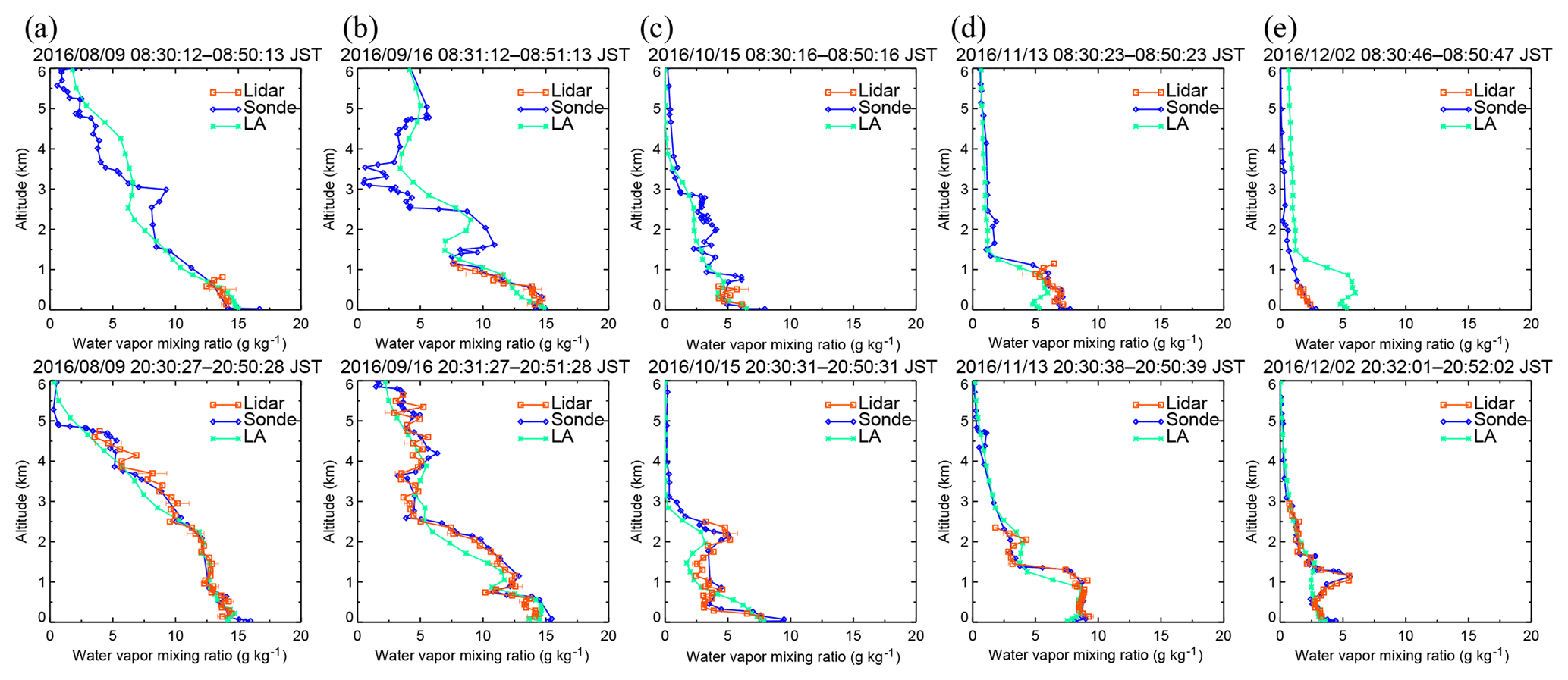
Figure 9 Vertical distributions of water vapor mixing ratios obtained with the MRL (orange) and radiosondes (blue) compared with local analysis data (green) for 08:30 LST (upper panel) and 20:30 LST (bottom panels) on (a) 9 August, (b) 16 September, (c) 15 October, (d) 13 November, and (e) 2 December 2016.

To test the long-term stability of the MRL system, we operated it for 4 months, from 2 August to 6 December 2016. After QC of the MRL data, the maximum measurement height was mostly ∼1 km during the day throughout the measurement period, whereas at night when low, thick clouds were absent, it decreased from 6 to 2.5 km over the measurement period (Fig. 8). We attribute this nighttime decrease to (1) a drop by almost half in the power of the laser transmitter during its continuous operation for 3 months, which caused the SNR of the signals to decrease, and (2) decreases in the water vapor concentration from summer to winter in the lower troposphere, which caused a decrease in the strength of Raman backscatter water vapor signals. As for the laser power, it increased from 110 to 220 mJ pulse⁻¹ after replacing the flash lamp and adjusting the angles of the second and third harmonic crystals on 8 December 2017. As for the water vapor concentration, the monthly mean w values decreased from 17 to 4 g kg⁻¹ at 1000 hPa and from 8 to 1 g kg⁻¹ at 700 hPa between August and December in 2016.

In general, vertical distributions of w obtained with the MRL system agreed well with radiosonde measurements (Fig. 9). However, the MRL- and radiosonde-derived values sometimes differed considerably from LA data for the same dates (e.g., between 2.5 and 3.5 km at 20:30 LST on 9 August, between 1.5 and 2.5 km at 20:30 LST on 16 September, and between 0.5 and 1.2 km at 20:30 LST on 2 December 2016). More detailed analysis will be given in Sect. 3.3.

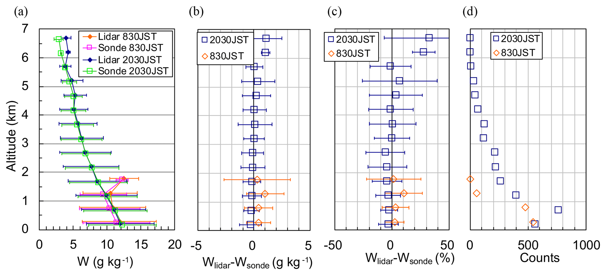
Figure 10 Vertical variations in (a) mean w_Lidar values (diamonds) and w_Sonde (open squares) values at intervals of 500 m for 20:30 and 08:30 LST from 2 August to 6 December 2016, and their (b) absolute and (c) relative differences. Symbols and error bars in (a)–(c) show means and standard deviations. (d) The number of data points at each altitude.

To study the height dependence of the difference (w_Lidar−w_Sonde), we examined the vertical variation in the mean difference at intervals of 500 m (Fig. 10). The mean difference was less than 1 g kg⁻¹ (10 %) below an altitude of 6 km at night and below 1 km in the daytime. Above these altitudes, the MRL values were higher than the radiosonde-derived values. Possible reasons for the larger differences at higher altitudes are (1) the small number of data points in those regions (Fig. 10d), which caused the statistical significance to be low, (2) the difference in the air parcel measured by the two instruments, because as they ascended the radiosondes were sometimes blown several kilometers or more from the MRL position by horizontal winds, particularly above an altitude of 6 km at night, and (3) the generation of spurious Raman signals above 1 km by high solar background radiation in the daytime, as will be discussed in Sect. 3.1.2. The influence of the temperature dependence of the Raman cross section (e.g., Whiteman, 2003) is negligible for the MRL because the variation is estimated to be 0.5 % for the temperature range of 253–303 K.

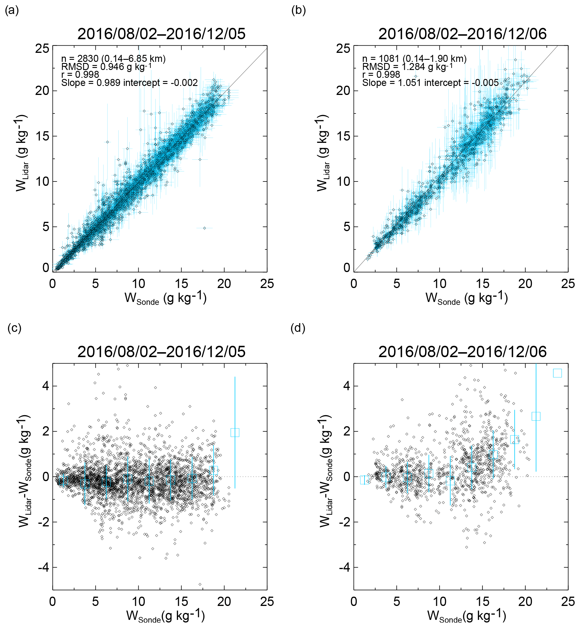
Figure 11 (a, b) Scatter plots of w obtained with the MRL (w_Lidar) versus w obtained with radiosondes (w_Sonde) at (a) 20:30 LST and (b) 08:30 LST from 2 August to 6 December 2016. (c, d) Scatter plots of the difference (w_Lidar−w_Sonde) as a function of w_Sonde at (c) 20:30 LST and (d) 08:30 LST. Blue symbols show the means, and the blue lines show the standard deviations of the difference at intervals of 2.5 g kg⁻¹. Data points with an MRL measurement uncertainty of less than 30 % are plotted.

3.1.2 Scatter plot comparison

After the data were screened for QC, we compared w values obtained with the MRL and by radiosonde from 2 August to 6 December 2016 in 110 vertical profiles for 20:30 LST and 113 for 08:30 LST (Fig. 11). For this comparison, the radiosonde data were linearly interpolated to the heights of the MRL data. Note that the maximum altitude of the comparison for 08:30 LST (1.9 km) was lower than that for 20:30 LST (6.85 km) because, owing to their large uncertainty, daytime data at higher altitudes were excluded by the QC screening. The MRL-derived w (w_Lidar) values agreed with the radiosonde-derived values (w_Sonde) over the range from 0 to 20 g kg⁻¹ (Fig. 11). A geometric mean regression analysis conducted by assuming that $w_{\mathrm{Sonde}}=\text{slope}\times w_{\mathrm{Lidar}}+\text{bias}$ yielded a slope of 0.989 with the statistical uncertainty of ±0.002 and an intercept of $-\mathrm{0.002}\pm \mathrm{0.018}$ for the 20:30 LST (Fig. 11a) and a slope of 1.051±0.004 and an intercept of $-\mathrm{0.005}\pm \mathrm{0.053}$ g kg⁻¹ for 08:30 LST (Fig. 11b). To examine the dependence of the difference in w (w_Lidar−w_Sonde) on the magnitude of w_Sonde, we plotted (w_Lidar−w_Sonde) as a function of w_Sonde, as well as the means and standard deviations of (w_Lidar−w_Sonde), at intervals of 2.5 g kg⁻¹ (Fig. 11c and d). As a result, we found no significant bias in the difference for w_Sonde ranging from less than 20 g kg⁻¹ at night to less than 15 g kg⁻¹ in the daytime (i.e., mean differences were smaller than 0.3 g kg⁻¹). In contrast, we found positive biases for larger w_Sonde value ranges; the bias was 1.7 g kg⁻¹ at 08:30 LST for w ranging from 17.5 to 20 g kg⁻¹. A possible reason for the daytime bias at high values of w_Sonde is that high solar background radiation generated spurious noise spikes and high photon counts in Raman water vapor signals above an altitude of 1 km that were not rejected by QC. We are investigating the method to reject such data by QC, although they have small impacts on the water vapor fields analyzed from the data assimilation because their measurement errors are large.

3.2 Comparison with GNSS PWV data

To validate the MRL measurement data for times when coincident radiosonde data were unavailable, we compared the MRL-derived precipitable water vapor (PWV) with PWV values obtained from GNSS data. The GNSS receiver was located 80 m west of the MRL. It observed the carrier phase transmitted by GNSS satellites from which the PWV was estimated with a temporal resolution of 5 min during the validation period. The PWV value represents the vertically integrated water vapor content averaged over a horizontal distance of approximately 20 km around the antenna. See Shoji et al. (2004) for more details of the derivation method. To obtain PWV from the MRL data, we computed the vertical profile of the water vapor density from MRL-derived w and atmospheric density obtained by the radiosonde closest in time to the MRL measurement period, and we vertically integrated the water vapor density from an altitude of 0.1 km to the maximum height with a measurement uncertainty of less than 30 %. Below 0.1 km, we interpolated the w data to the ground level in situ measurement. Then we compared the temporal variations in PWV obtained with the MRL with those obtained from GNSS data from August to December 2016 (Fig. 12). So that this comparison would be meaningful, we excluded MRL data obtained when the maximum measurement height was lower than 5 km; as a result, mostly nighttime lidar values obtained when low, thick clouds were absent were used in the comparison. The temporal resolution of the GNSS data was reduced by averaging from 5 min (original GNSS resolution) to 20 min to match the resolution of the MRL data.

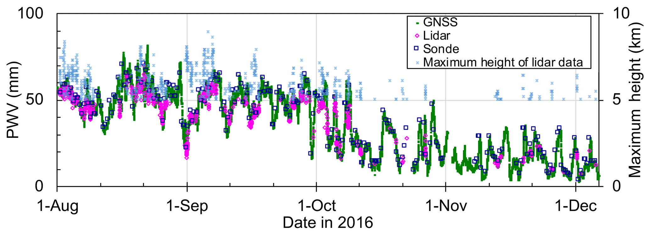
Figure 12 Temporal variations in PWV obtained with lidar (magenta diamonds), GNSS (green dots), and radiosonde (blue squares) from 2 August to 6 December 2016 over Tsukuba. Data with measurement uncertainties of less than 10 % that were obtained when the maximum MRL measurement height exceeded 5 km (light blue asterisks) are plotted.

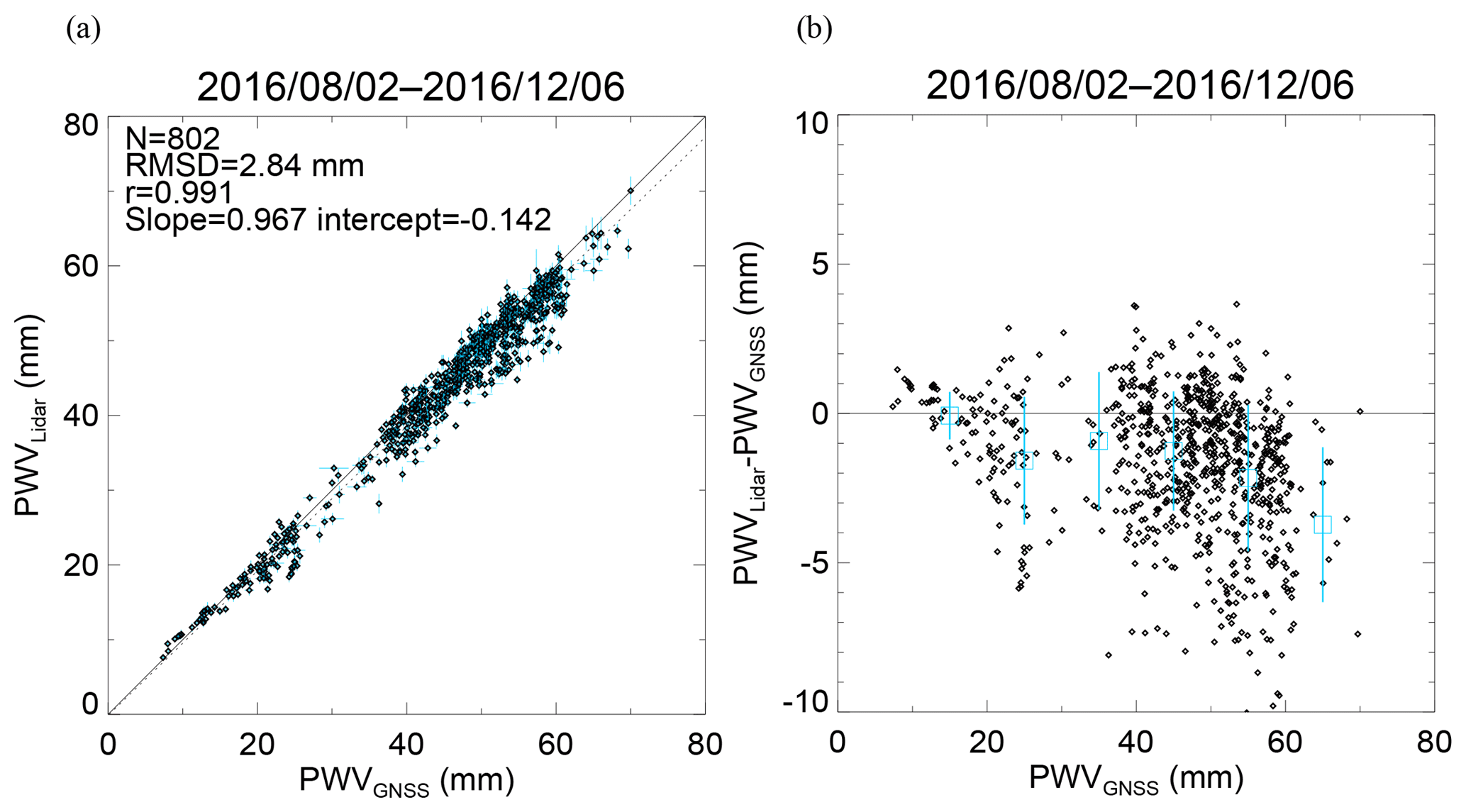
Figure 13 Scatter plots (a) of PWV obtained with the MRL system against PWV obtained from GNSS data from 2 August to 6 December 2016 and (b) their difference (PWV_Lidar−PWV_GNSS) versus PWV_GNSS. In (b), the open squares and vertical lines show the means and standard deviations of the difference at intervals of 10 mm.

The temporal variation in MRL-derived PWV was similar to that of the GNSS-derived PWV (Fig. 12). In summer (August–September), when a moist air mass from the Pacific Ocean covered the observation area, the PWV values were mostly higher than 30 mm. In autumn and winter (October–December), when a dry air mass from the Asian continent prevailed, the PWV values were mostly lower than 20 mm. We note that the number of available lidar PWV data was smaller in autumn and winter than in summer because the decrease in the laser power as mentioned before (Sect. 3.1.1) and because in autumn and winter the Raman backscatter signal tends to be weakened by the low water vapor concentration in the middle troposphere. The regression analysis of PWV derived from MRL data against GNSS-derived PWV showed a strong positive correlation (correlation coefficient 0.991; Fig. 13a) between them, but many of the MRL-derived PWV values were lower, most by up to 5 mm, than the GNSS-derived values (Fig. 13b). The most plausible reason for the lower MRL-derived PWV values is that the MRL did not always measure the entire water vapor column. In addition, both positive and negative differences could be caused by the measured air masses being different (see Sect. 3). The difference in PWV would be large if large horizontal inhomogeneity of the water vapor concentration existed in the observation area. Shoji et al. (2015) utilized the slant path delay of the GNSS signal to estimate the horizontal inhomogeneity of water vapor on a scale of several kilometers around the measurement site. The use of a technique that combines MRL and GNSS observations for monitoring the vertical and horizontal distributions of water vapor holds promise, and the development of such a technique is our future task.

3.3 Comparison with local analysis data

We compared hourly MRL values of w with LA data because the primary purpose of our MRL measurement was to improve the initial condition of the water vapor field of the NWP model. The LA consists of hourly meteorological data with a horizontal resolution of 2 km over Japan provided by the JMA. These data are obtained by a three-dimensional variational (3D-var) data assimilation technique from hourly observation data from multiple sources, including surface measurements, satellites, and GNSS-derived PWV data. LA data provide initial conditions to local-scale NWP models used for 9 h forecasts for aviation, weather warnings and advisories, and very short-range precipitation in and around Japan, provided every hour. The vertical resolution of the LA data is 45–868 m with 48 layers. See JMA (2017) for more details about the LA data.

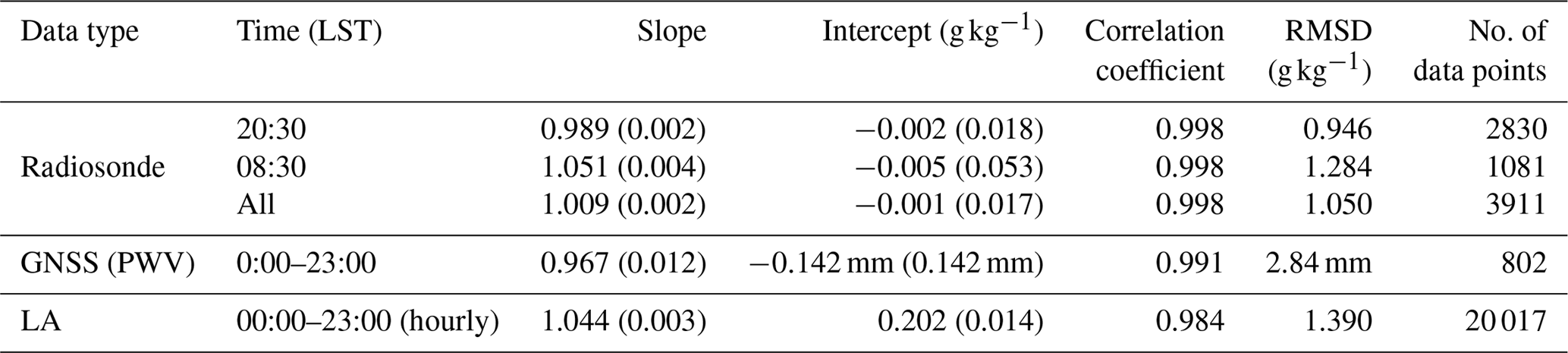
Table 2 Results of water vapor measurements by the MRL compared with data obtained by other instruments or from local analyses. Values in the parentheses of slope and intercept are the statistical uncertainties.

3.3.1 Vertical distributions

Our comparison of vertical variations in w obtained with the MRL system with w derived from the LA (Fig. 9) showed higher values of the MRL than the LA data. The statistics of the comparison showed that the MRL values were higher by up to 1.1 g kg⁻¹ (25 %) over the entire altitude range (Fig. 15). In addition, the magnitude of the difference (w_Lidar−w_LA) was larger than the difference with radiosonde values (w_Lidar−w_Sonde) (Fig. 10). This result suggests that the assimilation of MRL data has the potential to improve the initial conditions provided to the NWP model.

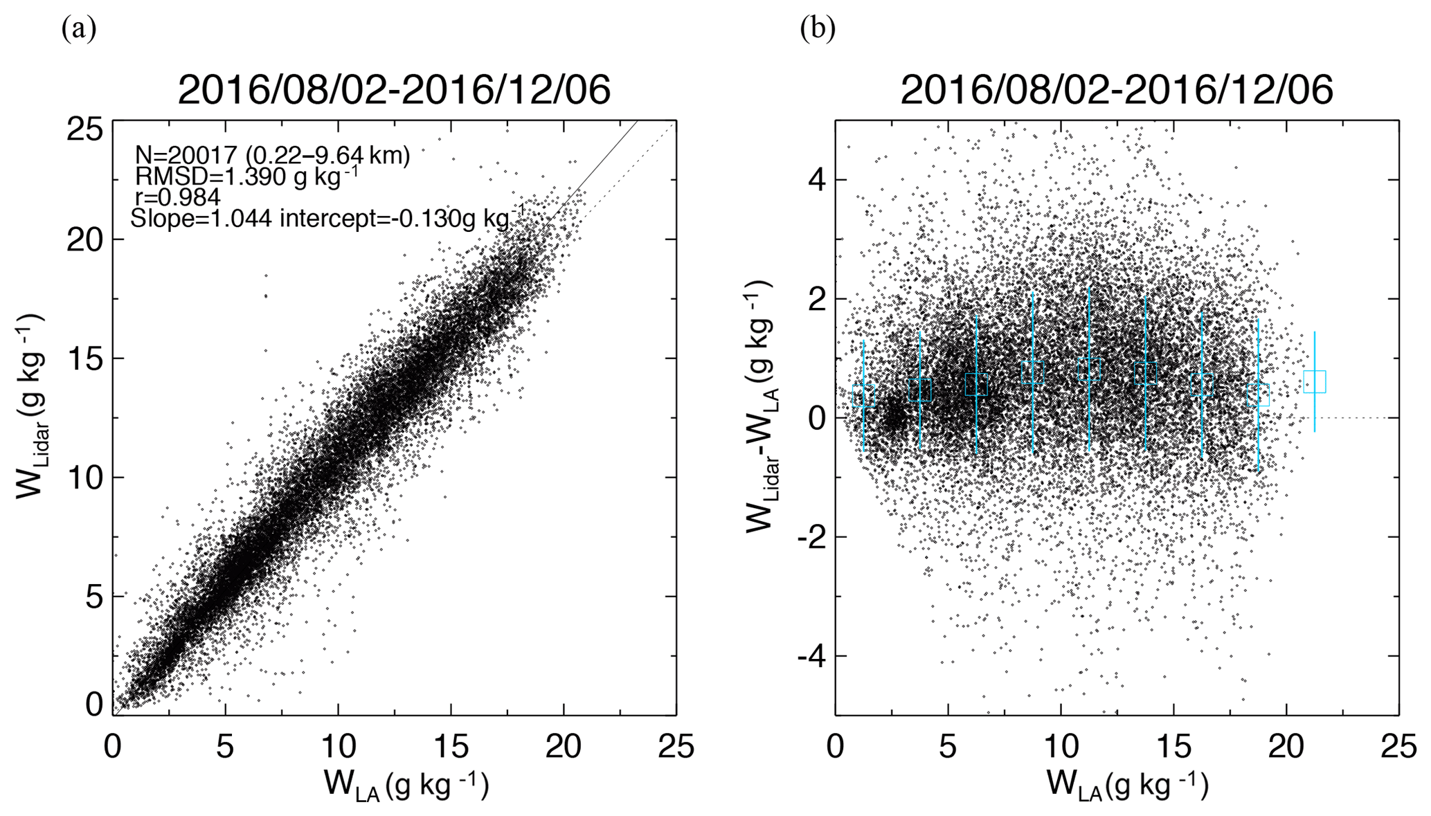
Figure 14 Scatter plots of (a) w obtained with the MRL (w_Lidar) versus w obtained from the local analysis (w_LA) and (b) their difference (w_Lidar−w_LA) as a function of w_LA from 2 August to 6 December 2016. In (b), the blue open squares and vertical lines show means and standard deviations of the difference at intervals of 2.5 g kg⁻¹.

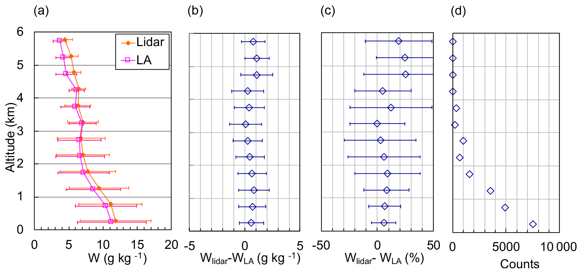
Figure 15 Vertical variations in (a) mean values and standard deviations of w obtained with the MRL (w_Lidar) and from the local analysis (w_LA) at 500 m intervals and their (b) absolute and (c) relative differences from 2 August to 6 December 2016. Symbols and error bars in (b) and (c) show the means and standard deviations of the difference. (d) The number of data points at each altitude.

3.3.2 Scatter plot comparison

Figure 14 shows the scatter plot of w obtained with MRL. For this comparison, the MRL data were linearly interpolated to the heights of the LA data. The result revealed that the root-mean-square difference (RMSD) (1.390 g kg⁻¹) was larger than that obtained when we compared MRL values with nighttime radiosonde values (0.989 g kg⁻¹; Fig. 11a). Moreover, the MRL-derived w values were consistently higher, by 0.2–0.8 g kg⁻¹ (1 %–11 %) than those derived by LA for w in the range of 0–22.5 g kg⁻¹ (Fig. 14b). We also compared LA data with the radiosonde data for the same period (not shown) and found that the mean LA data at intervals of 2.5 g kg⁻¹ differed from the radiosonde data by −0.2 to 0.9 g kg⁻¹ (3 %–11 %). We infer that the LA data used in this comparison had a negative bias because the accuracy of the radiosonde relative humidity measurements was 5 %–7 %. The differences with the LA data can be related to local effects and thus to the representativeness of the measurement site at the mesoscale. They can also be due to a problem in the assimilation process if it does not integrate the error matrices well.

3.4 Summary of the validation results and outlook

Table 2 summarizes the results of our comparisons of water vapor measurements obtained by the MRL and other instruments or local analyses. The correlation was highest and the RMSD was smallest when MRL-derived w was compared with w obtained by radiosonde at night. This result was probably because (1) the MRL system was calibrated by using radiosonde data, (2) the instruments measured the same quantity (w), and (3) the measurement performance of the MRL was best at night. The agreement with radiosonde data was not as good in the daytime as it was at night because the measurement uncertainty of w was larger in the daytime, even though the slope and intercept of the regression analysis did not differ significantly between daytime and nighttime measurements. The MRL-derived PWVs at night were slightly lower than those derived from GNSS data because of the measurement range limitation of the MRL system. The regression analysis of MRL-derived w versus LA data showed that the magnitudes of the deviation of the slope from 1 and the deviation of the intercept from zero were larger than those obtained in the analysis with radiosonde data, and the correlation coefficient was the lowest among the comparisons. From these results, we can expect that assimilation of MRL-derived w after QC can improve the initial conditions of the NWP model for heavy rain forecasting. In fact, a first data assimilation experiment of the MRL-derived vertical profiles of w into the JMA NHM using the three-dimensional LETKF for the heavy rainfall forecasting has been reported by Yoshida et al. (2018), who showed a positive impact on the analyzed and forecasted humidity fields on the Kantō Plain on 17 August 2016. More detailed description of the assimilation experiments will follow soon (Yoshida et al., 2019).

Despite the potential usefulness of the MRL-measured data for weather forecasting, the MRL cannot measure the water vapor inside and above optically thick clouds. To overcome this disadvantage, it is important to use synergistic approaches with different instruments such as GNSS, microwave radiometer, and radiosonde to measure the water vapor distribution even under cloudy conditions (e.g., Foth and Pospichal, 2017).

4 Conclusion

We developed a low-cost automated compact mobile Raman lidar system for measuring the vertical distribution of the water vapor mixing ratio w in the lower troposphere that is easy to be deployed to remote sites and is capable of unattended operation for several months. Our comparison of the MRL-derived w values with those obtained with collocated radiosondes showed that they agreed within 10 % and RMSD with 1.05 g kg⁻¹ between altitudes of 0.14 and 5–6 km at night and between altitudes of 0.14 and 1.5 km in the daytime. The calibration coefficient of the MRL showed no significant temporal variation during 4 months of continuous operation in 2016. A small correction for beam overlap was necessary below 0.5 km. The MRL-derived precipitable water vapor values obtained at night when low clouds were absent and the maximum heights of the MRL measurement exceeded 5 km were slightly lower than those obtained from GNSS data. The fact that the MRL-derived w values were at most 1 g kg⁻¹ (25 %) larger than those in the local analysis data suggests that assimilation of the MRL data can improve the initial condition of the water vapor distribution in the lower troposphere of the NWP model. Although the MRL system was originally developed for heavy rain forecasting, it can also be utilized for the study of water vapor in the lower troposphere such as boundary layer structure and cloud formation.

The measurement altitude of the current Raman lidar system is limited to 1.5 km in the daytime. Although this limitation might not preclude the use of data from the system for heavy rain forecasting and the other applications, it would be better to expand the measurement height. To detect water vapor in the middle troposphere in the daytime, a diode laser-based differential absorption lidar might be useful because it can continuously measure the water vapor concentration up to an altitude of 3 km both in the daytime and at night (Repasky et al., 2013; Spuler et al., 2015; Phong Pham Le Hoai et al., 2016).