the Creative Commons Attribution 4.0 License.
the Creative Commons Attribution 4.0 License.
 | 21 Jun 2019
Relationship analysis of PM2.5 and boundary layer height using an aerosol and turbulence detection lidar
Chong Wang
Mingjiao Jia
Yunbin Wu
Tianwen Wei
Xiang Shang
Chengyun Yang
Xianghui Xue
Xiankang Dou
The atmospheric boundary layer height (BLH) is a key parameter in weather forecasting and air quality prediction. To investigate the relationship between BLH and air pollution under different conditions, a compact micro-pulse lidar integrating both direct-detection lidar (DDL) and coherent Doppler wind lidar (CDWL) has been built. This hybrid lidar is operated at 1.5 µm, which is eye-safe and made of all-fibre components. The BLH can be determined from aerosol density and vertical wind independently. During a 45 h continuous observation in June 2018, the stable boundary layer, residual layer and convective boundary layer are identified. The fine structure of the aerosol layers, drizzles and vertical wind near the cloud base are also detected. In comparison, the standard deviation between BLH values derived from DDL and CDWL is 0.06 km, indicating the accuracy of this work. The retrieved convective BLH is a little higher than that from ERA5 reanalysis due to different retrieval methods. Correlation between different BLH and PM2.5 is strongly negative before a precipitation event and becomes much weaker after the precipitation. Different relationships between PM2.5 and BLH may result from different BLH retrieval methods, pollutant sources and meteorological conditions.
- Article
(8298 KB) - Full-text XML
- BibTeX
- EndNote


In recent decades, with rapid urbanisation, air pollution has become a severe environmental problem in China (Chan and Yao, 2008; Li et al., 2016; Song et al., 2017; Zhang et al., 2012). Particulate matter (PM) with an aerodynamic diameter less than 2.5 µm (PM2.5) attracts public attention due to its adverse effects on human health and the environment (Brunekreef and Holgate, 2002; Cohen et al., 2017; Huang et al., 2014; Kampa and Castanas, 2008). In addition to pollutant emissions and topographic conditions, the spatial and temporal distribution of PM is mainly affected by meteorological conditions in the troposphere, especially in the atmospheric boundary layer (ABL) (Chen et al., 2018; Z. Li et al., 2017; Song et al., 2017; Su et al., 2018; Wei et al., 2018).
The ABL, also called the PBL (planetary boundary layer), plays an important role in the lower troposphere. The ABL is directly influenced by and responds to the Earth's surface activities, such as frictional drag, evaporation, transpiration and heat transfer, on a timescale of an hour or less (Stull, 1988). The ABL consists of three major parts during the diurnal evolution: the convective boundary layer (CBL), stable boundary layer (SBL) and residual layer (RL) (Stull, 1988). The ABL is a key factor in the control and management of air quality, numerical weather prediction, urban and agricultural meteorology, aeronautical meteorology, hydrology, and so on (Large et al., 1994). Pollutants or any constituents within this layer are fully mixed and vertically dispersed due to convection or mechanical turbulence (Seibert, 2000). The boundary layer height (BLH) determines the volume available for pollution dispersion and transport in the atmosphere. Low BLH and weak turbulence strengthen the accumulation of air pollutants (Miao et al., 2018; Petaja et al., 2016). Hence, the BLH is one of the fundamental parameters in dispersion models. A roughly anti-correlated relationship between PM2.5 and BLH has been found in recent years (Du et al., 2013; Miao et al., 2018; Petaja et al., 2016; Su et al., 2018). However, the relationship analysis of PM2.5 and BLH in the ABL derived by aerosol (static) and by turbulence (dynamical), respectively, is still rare. Therefore, continuous observation of the BLH with high temporal and spatial resolution and the relationship between pollution and BLH is desirable for air quality prediction.
There are always significant changes in vertical profiles of aerosol concentration, specific humidity, potential temperature or turbulence around the top layer of the ABL, making it possible to derive the BLH. There are several instruments used for the determination of BLH based on the sharp gradient in the vertical profiles mentioned above (Baars et al., 2008; Bonin et al., 2018; H. Li et al., 2017a; Seibert, 2000; Yang et al., 2017): for example, in situ instruments, such as radiosondes, balloons, masts, and aircraft, and remote sensing instruments, such as sodar, wind profilers, lidar, and ceilometers. All of these instruments have advantages and shortcomings regarding accuracy, detection range, and spatial and temporal resolution, as summarised by Seibert (2000). Among these instruments, the lidar system provides backscattering signal with a sufficient spatial and temporal resolution, a long enough detection range and high enough accuracy for determining the BLH. These qualities make lidar a powerful tool for BLH assessment.
In recent decades, lidar are widely used in the lower atmosphere via Mie scattering, Raman scattering and differential absorption (Campbell et al., 2002; Godin et al., 1989; Murray and van der Laan, 1978; Reitebuch, 2012; Renaut et al., 1980; Xia et al., 2007). Aerosol, trace gas concentration, atmospheric density, temperature and wind can be detected by these lidar. Recently, a micro-pulse direct-detection lidar (DDL) based on up-conversion technology was developed to make continuous measurements of aerosol in the troposphere (Xia et al., 2015). A coherent detection Doppler wind lidar (CDWL) was developed to measure wind field in the ABL (Wang et al., 2017). Different from traditional micro-pulse lidar operated at or near 532 nm (He et al., 2008; H. Li et al., 2017b; Sawyer and Li, 2013), these two lidar are operated at 1.5 µm, are eye-safe and can be made with all-fibre components. The 1.5 µm laser shows the highest maximum permissible exposure in the wavelength range from 0.3 to 10 µm (Xia et al., 2015). The invisible infrared eye-safe laser makes these two lidar able to horizontally operate in a densely populated city . The all-fibre structure makes these lidar robust and immune to external environment changes such as vibration and temperature. Based on these two lidar, BLH values can be derived from both aerosol density and turbulence. The simultaneous implementation of DDL and CDWL will improve the precision of BLH assessment and enrich the meteorological data in the ABL.
Generally, DDL and CDWL belong to different lidar categories. In this work, a hybrid lidar integrating both systems is developed for simultaneous measurements of aerosol and vertical wind. The integrated lidar is utilised to further understand the relationship between PM2.5 and BLH. The integrated lidar system, meteorology and PM data are described in Sect. 2. The retrieval methods of BLH are briefly introduced in Sect. 3. In Sect. 4, the results of and discussions about lidar data, the retrieved BLH and the relationship between PM2.5 and BLH are presented. Finally, the conclusion and summary are drawn in Sect. 5.
2.1 The integrated lidar system
A compact and integrated micro-pulse lidar system is developed. Benefiting from all-fibre configuration and up-conversion technology, the lidar inherits advantages from both DDL and CDWL. The DDL is based on up-conversion technology and is used for long-range aerosol measurement (Xia et al., 2015). The CDWL is used for wind field measurement (Wang et al., 2017). Two lidar systems use only one set of instruments comprised of a laser source, optical collimator and control system. The unique optical telescope guarantees that the measured signal in both systems is from the same backscattering volume and that the radial wind profile and aerosol concentration are measured simultaneously.
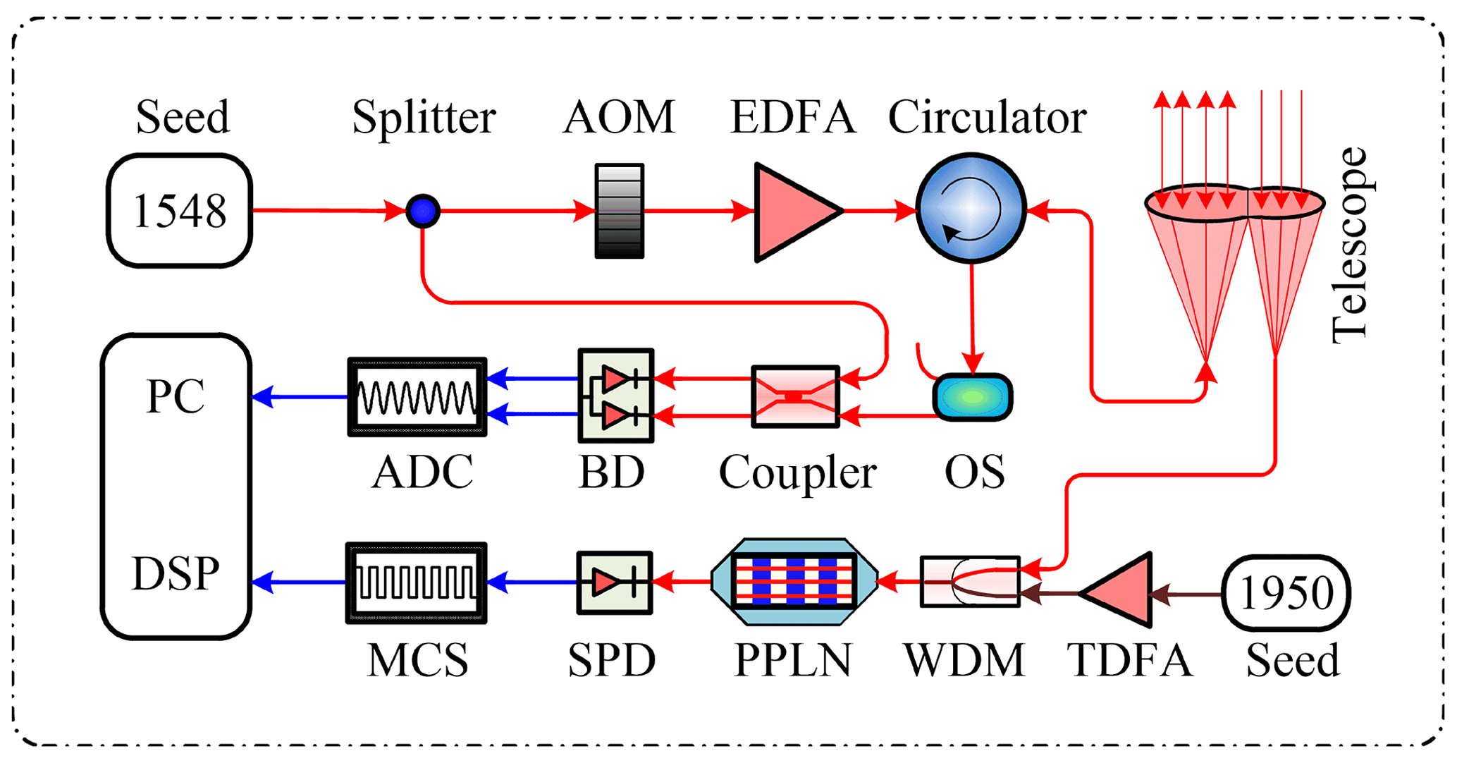
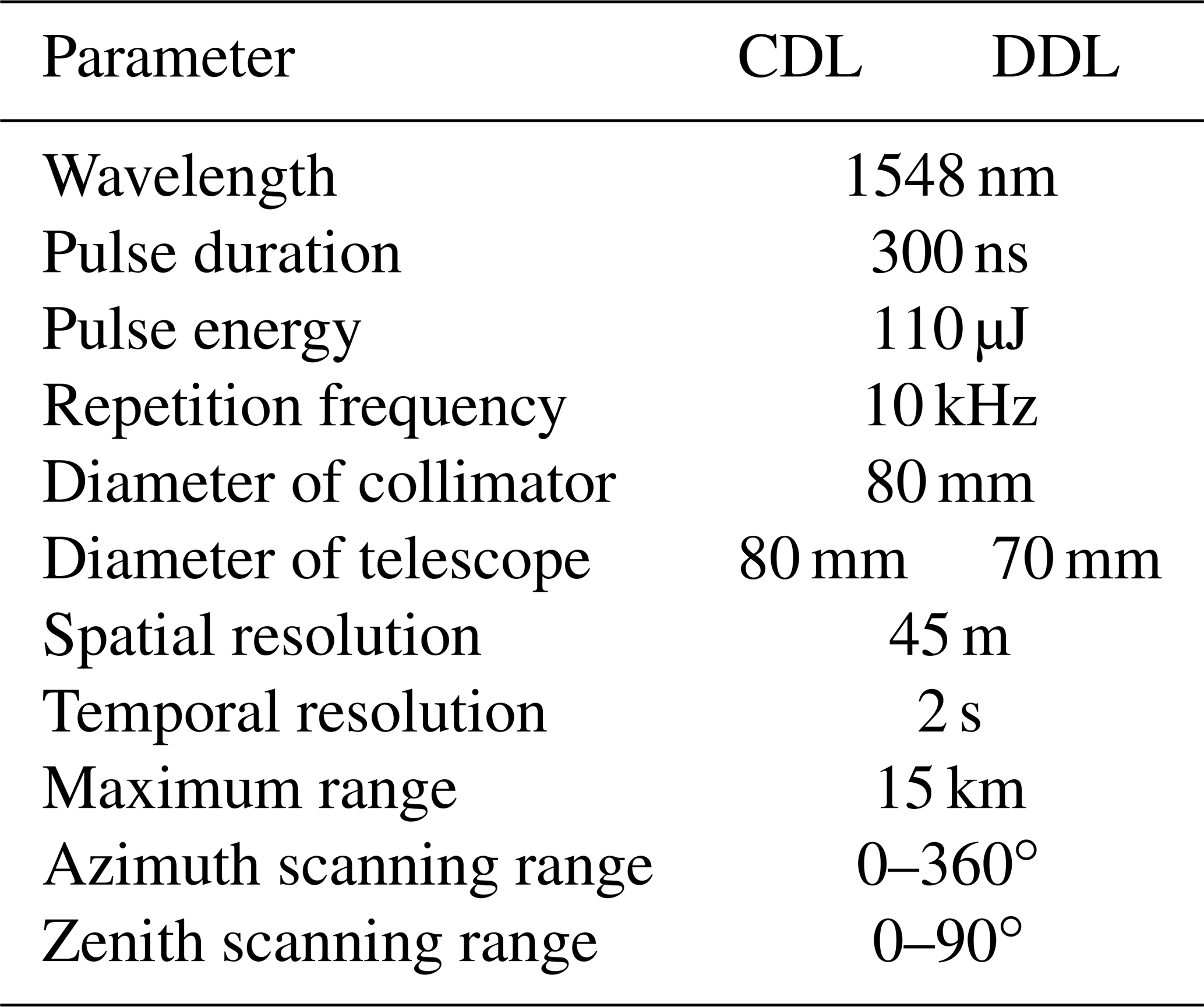
The diagram of the system is shown in Fig. 1. The seed laser emits a continuous wave (CW) at 1548 nm, then the CW is split into the local oscillator and transmitted seed laser by a beam splitter (BS). The transmitted seed laser is chopped and frequency-shifted 80 MHz by an acousto-optical modulator (AOM). After the AOM, the transmitted laser is amplified by an erbium-doped fibre amplifier (EDFA) and transmitted into the atmosphere via a collimator. The pulse duration is 300 ns and the pulse energy is 110 µJ. The atmospheric backscattering is collected by two telescopes, adopting a double “D” configuration. As shown in Fig. 1, the two aspheric lenses are glued together with parallel optical axes for easy alignment and to avoid a blind zone. The absolute overlap distance is 1 km. On the CDWL channel, the backscattering pass through a circulator is chopped by an optical switch (OS), which cuts off the reflection light from the circulator and lens. The reflection light is much higher than the atmospheric backscattering and will cause saturation and even breakdown in the balanced detector (BD). After the OS, the backscattering is mixed with a local oscillator and measured on the BD. The analogue signal is converted to digital signal by an ADC and then processed by a PC. On the DDL channel, the backscattering is collected and mixed with a pump laser at 1950 nm in a wavelength division multiplexer (WDM). The mixed laser then passes through the periodically poled lithium niobate waveguide (PPLN). The backscattering at 1548 nm is converted to 863 nm by the PPLN and detected by a silicon single-photon detector (SPD). A filter is used to filter out the noise. A multi-channel scaler (MCS) records the digital signal. Benefiting from coherent detection and the narrow passband of the PPLN, this integrated lidar can perform all-day detection of the atmosphere. The detailed parameters of the integrated lidar are listed in the Table 1.
During the experiment, the integrated lidar is pointed vertically. Then the vertical wind and backscattering intensity are measured simultaneously. The raw DDL data are recorded with a spatial and temporal interval of 45 m and 2 s, respectively, while CDWL data are 60 m and 2 s, respectively. The integrated lidar is deployed 5 m above ground on the campus of the University of Science and Technology of China (USTC, 31.84∘ N, 117.26∘ E), an urban area in Hefei, China.
2.2 Meteorology and PM2.5 data
A weather transmitter (Vaisala WXT520) is used to measure meteorological parameters, including temperature, relative humidity, liquid precipitation, barometric pressure, wind velocity and direction. A visibility sensor (Vaisala PWD50) is used to measure the atmospheric visibility. A wide-range aerosol spectrometer (Grimm Mini WRAS 1371) measures aerosol volume size distribution ranging from 10 nm to 35 µm over 41 channels (Shang et al., 2018). Then PM2.5 and PM10 values are calculated. All of these instruments were deployed 60 m above ground and 250 m east of the integrated lidar on the top of a research building in USTC. During the experiment, all of these meteorological data are recorded with an interval of 1 min.
The BLH is retrieved from both aerosol concentration and vertical wind in this experiment. For the DDL data, the range-corrected lidar signal (RCS), N(R)R2, has a sharp decrease at BLH, where N(R) is the backscattering photon number from an altitude of R. As for the CDWL, the temporal vertical velocity variation in the ABL is much stronger than that in the free atmosphere. The carrier-to-noise ratio (CNR) of the CDWL also represents the aerosol concentration, which can also be used to determine the BLH.
The Haar wavelet covariance transform (HWCT) method is used to retrieve BLH from aerosol concentration. The HWCT Wf(a,b) is defined as follows (Brooks, 2003):
with the Haar function:
where f(z) is the normalised RCS or CNR, zb and zt are the bottom and top height of a selected range, a is the dilation of the Haar wavelet, and b is the centre position of the Haar function. For a given dilation, the height where maximum Wf(a,b) appears is considered to be the BLH. Considering different vertical spatial resolutions and having tested multiple values of dilation, a dilation of 150 and 250 m is applied for RCS and CNR, respectively, for these 45 h observations. Compared with the gradient method, the HWCT method has greater adjustability and robustness (Korhonen et al., 2014). The interference by multiple aerosol layers in the ABL is negligible for an appropriate dilation. In order to reduce the interference from unexpected noise, the signal is averaged to a temporal resolution of 1 min in BLH determination. It should be noted that the cloud layer could affect the BLH results. An upper limit is set to the HWCT method for higher clouds. For the scattered stratocumulus that may exist in the capping layer, the differences between cloud top and BLH are relatively small. In addition, the duration time of stratocumulus is also short in the field of view of the lidar. Thus, the influence of scattered stratocumulus is negligible. The low-level cloud in the ABL can be identified by where the paired minimum Wf(a,b) and maximum Wf(a,b) occur at heights close to each other. The BLH cannot be retrieved under these conditions. As described in Sect. 2.1, RCS should be corrected with an overlap factor before the analysis. As an example, the measured RCS and CNR after a 1 min average (after overlap correction and background noise deduction) at 10:40 LT, 1 June 2018 is shown in Fig. 2a. The corresponding HWCT results are shown in Fig. 2b, from which the BLH can be determined.
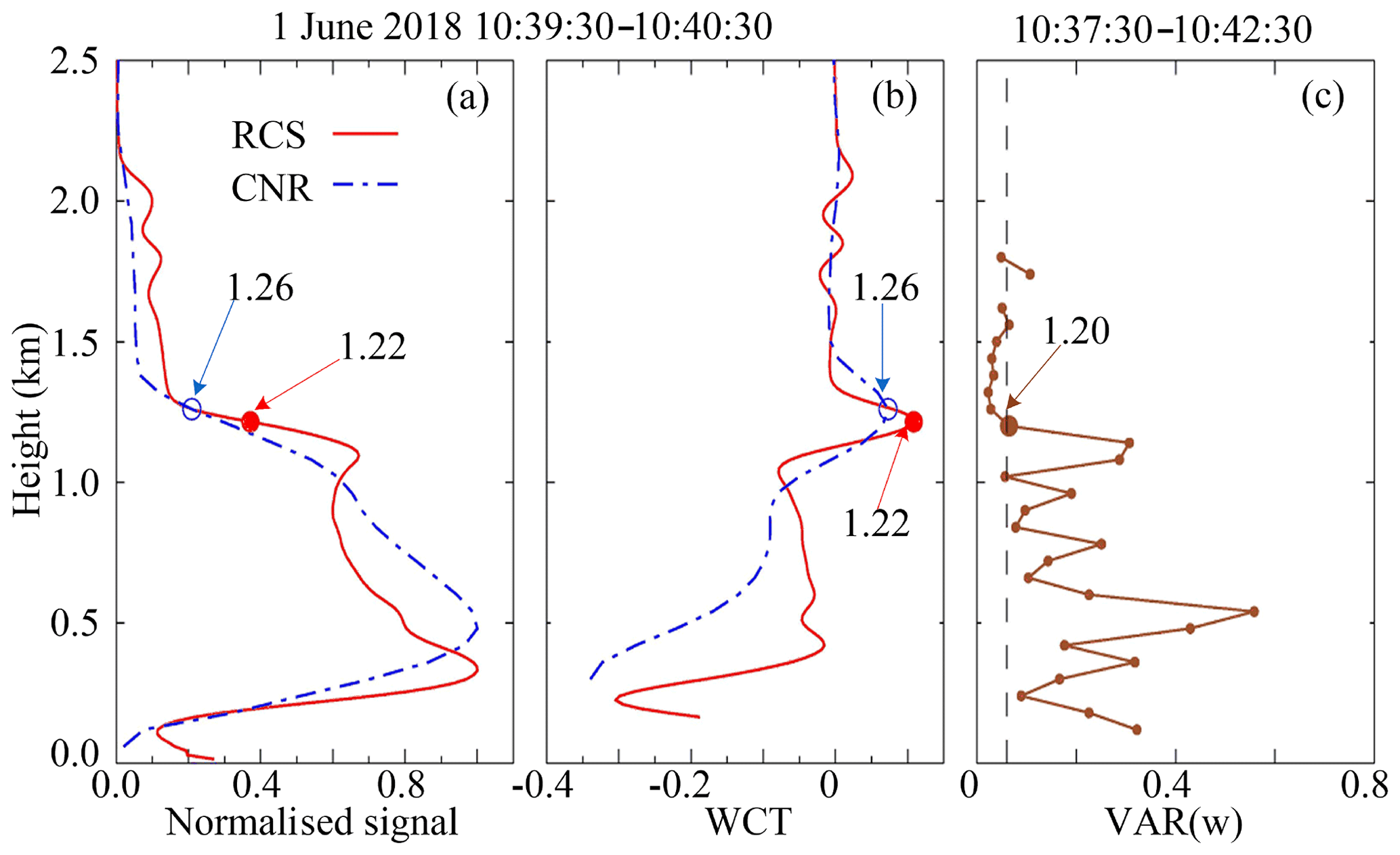
Figure 2(a) The 1 min mean normalised RCS and CNR profiles. (b) The corresponding HWCT results of the RCS and CNR profiles in (a). (c) The vertical velocity variance profile. The dashed black line indicates the threshold of 0.06 m2s−2. The red solid circle, blue circle and brown solid circle denoted by the arrows indicate the retrieved BLH, with the values at the end of the arrows.
The BLH can also be determined from the variance of vertical velocity , which represents the vertical component of the turbulence kinetic energy. For a given time window and a reliable threshold, below the BLH, the is larger than the threshold and vice versa. The threshold varies from different locations (Huang et al., 2016). In this study, the threshold is set to be 0.06 m2 s−2, which is suitable, as shown in Fig. 2c. A median algorithm is used to mitigate the interference and fluctuation from unexpected turbulence and noise in the free atmosphere. The process is completed as follows: (1) select all the height with less than the threshold; (2) find the median height zm selected in (1); and (3) find the BLH, which is the maximum height below zm that larger than the threshold. An example of employing this threshold and algorithm is shown in Fig. 2c. Some confusing points, such as that at ∼1.0 and ∼1.6 km in Fig. 2c, can be distinguished.
Reanalysis data are always used in climatological and regional analysis of BLH (Collaud Coen et al., 2014; Guo et al., 2016; Seidel et al., 2012). ERA5 is the newest generation of ECMWF (European Centre for Medium-Range Weather Forecasts) atmospheric reanalysis of the global climate. ERA5 reanalysis assimilates a variety of observations and models in 4-D. The data have 137 levels from the surface up to 80 km altitude, the horizontal resolution is 0.3∘ for both longitude and latitude (Hersbach and Dee, 2016). The hourly BLH from high-resolution-realisation sub-daily deterministic forecasts of ERA5 is used to cross-check the BLH retrieved from lidar since there is no sounding data in Hefei. The BLH in ERA5 is determined by the bulk Richardson number (Rib) method (ECMWF, 2017; Seidel et al., 2012; Vogelezang and Holtslag, 1996). The bulk Richardson number Rib is defined as follows (Vogelezang and Holtslag, 1996):
Here g is the acceleration of gravity; h is height; θv0 and θvh are the virtual potential temperature at the surface; and h, uh, and vh are component wind speeds at h, respectively. The BLH is then defined as the lowest height where the Rib reaches a critical value of 0.25 (ECMWF, 2017).
Compared to the BLH retrieval, RL top can be identified through a simple rough threshold, which is described in the Appendix.
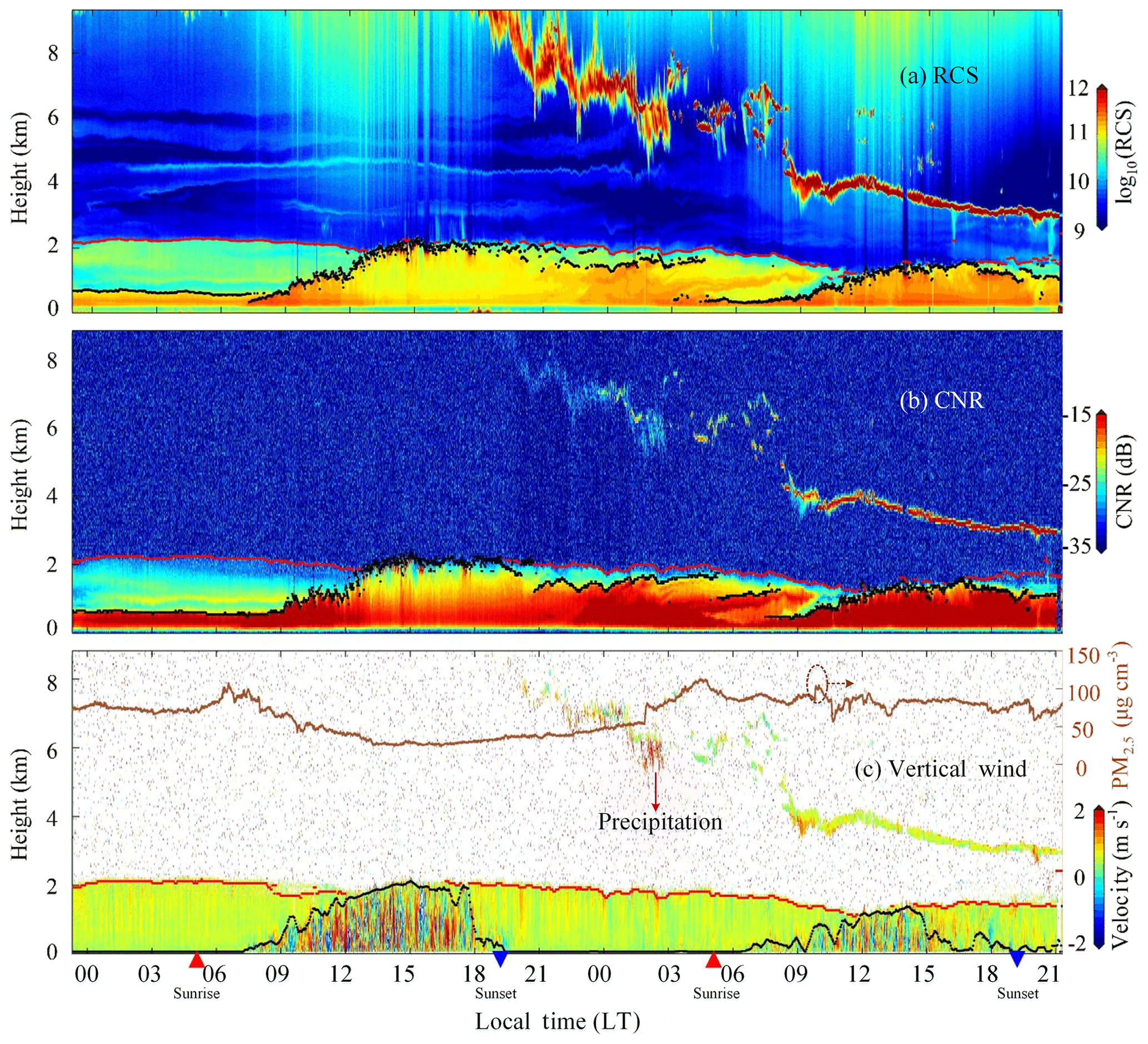
Figure 3Lidar observational results from 1 June 2018 to 2 June 2018. (a) The 1 min mean time series of logarithmic RCS profiles measured by DDL. The height time cross section of (b) CNR and (c) vertical wind measured by CDWL with 20 s temporal interval. The downward (upward) vertical wind is positive (negative). The dotted brown line indicates the PM2.5 concentration near the ground. The dotted black (red) lines in each panel indicate the BLH (RL tops) retrieved from RCS, CNR and vertical wind, respectively.
4.1 Observational results
Figure 3 shows a continuous observation over 45 h from 1 June to 2 June 2018. The RCS with 1 min temporal resolution and CNR and vertical wind with 20 s temporal resolution are shown. The dotted black line in each panel indicates the BLH derived from RCS, CNR and vertical wind, called BLHRCS, BLHCNR and BLHVAR in this study. Meanwhile, the dotted red lines in each panel indicate the RL tops. Sunrise and sunset times at 05:06 and 19:12 LT (local time) are marked by red triangles and blue inverted triangles. The experimental observation ends with rainfall on the ground on ∼2 June, 21:00 LT.
As shown in Fig. 3a, aerosol layer experiences a significant diurnal cycle within a height of 2 km. Before 09:00 LT on 1 June, an aerosol-derived SBL caused by radiative cooling from the ground can be easily found below ∼0.7 km with higher aerosol concentration than that in the RL. Subsequently, the ABL starts to grow due to solar heating after sunrise and deepens to a maximum height of about 2 km in the mid-afternoon. Sporadic stratocumulus appears at the top of the ABL with strong backscattering signal. During the night from 22:00 LT, 1 June to 06:00 LT, 2 June, the backscattering increases in the RL, which is related to the increase in aerosol concentration. After the sunrise on 2 June, the ABL grows as it did of 1 June, but the BLH is lower than that of 1 June.
The CNR measured by CDWL is shown in Fig. 3b. The evolution of the ABL is similar to that of RCS. The phenomena that are observed in RCS and described above can be also found in CNR. Figure 3c shows the height–time cross section of vertical wind. To guarantee the precision of the wind measurements, the data with CNR below −35 dB are abandoned (Wang et al., 2017). The downward vertical wind is positive and vice versa. Obviously, the convective ABL is well mixed with strong turbulence during the daytime between sunrise and sunset. Wave-like motions also exist in the nocturnal ABL associated with stratified atmosphere.
Cloud with strong backscattering can be detected between ∼3 and ∼9 km height by both DDL and CDWL. Corresponding vertical velocity of cloud is measured by the CDWL. Fine cloud structures above the ABL are shown in RCS with high spatial and temporal resolution due to higher detection efficiency. In addition, in the height ranging from ∼3 to ∼6 km on 1 June, several transport aerosol layers can be detected in RCS despite accompanying sunshine-induced noise. Interestingly, the transport aerosol layers meet the cloud base during the night on 1 June. The fine structures around the cloud base suggest the existence of drizzle. Moreover, precipitation in cloud can be identified by assuming that precipitation has a fall velocity greater than 1 m s−1 (Manninen et al., 2018). A precipitation case is indicated by the red arrow in Fig. 3c at approximately 02:00 LT, 2 June. The PM2.5 value measured simultaneously is illustrated as the dotted brown line in Fig. 3c. A sharp increase in PM2.5 occurs during the precipitation. These results hint at the potential applications of this integrated lidar in the investigations of aerosol–cloud–precipitation interactions.

Figure 4The simultaneous measured surface meteorological parameters during the experiment from 1 June 2018 to 2 June 2018. From (a) to (d) the parameters are (a) temperature and pressure; (b) wind velocity and wind direction; (c) visibility and relative humidity; and (d) logarithmic aerosol volume size, PM2.5, and PM10 concentration. The dashed vertical lines in (a)–(c) indicate the time when there is a sudden enhancement of PM2.5 in (d).
The simultaneous measurements of meteorological parameters including temperature, pressure, wind velocity, wind direction, visibility and relative humidity near the ground are shown in Fig. 4a–c. It should be noted that the building where the instrument is deployed would have an impact on these meteorological parameters. There is no precipitation event recorded on the ground by the weather transmitter, even during the precipitation in the cloud, as shown in Fig. 3c. Weak wind conditions (velocity less than 4 m s−1) during the whole experiment are not conducive to aerosol diffusion near the ground. The wind direction is always northerly despite the easterly wind before sunrise on 1 June. Two haze events occurred during this experiment, with visibility less than 10 km and relative humidity less than 80 %, (China Meteorological Administration, 2010). As mentioned before, there is a sudden increase in PM2.5 at approximately 02:00 LT, 2 June, during the precipitation. There are also sudden changes in relative humidity and visibility at the same time, indicated by the vertical dash-dotted lines. Simultaneous measurements of aerosol size volume distribution during this experiment are shown in Fig. 4d. The amount of aerosol rises in all size channels at LT, 2 June. Concentrations of PM2.5 and PM10 have almost the same evolution processes. It reveals that there is no specified single anthropogenic emission. The wet growth of the existing small particles caused by the precipitation above the ground may be responsible for the sudden increase in aerosols. Therefore, the experiment is chopped into two sections by the precipitation event, as the vertical dash-dotted lines show in Fig. 4.
4.2 BLH retrieval results
As shown in Fig. 3, the BLH results are well retrieved, indicating that the HWCT and variance methods are appropriate for BLH determination. An upper limit of 2.5 km of BLH is applied during the BLH retrieval. A comparison is performed, as shown in Fig. 5a, with retrieved BLHRCS, BLHCNR, BLHVAR and BLH from ERA5 (BLHERA5). The BLHRCS and BLHCNR are smoothed with median value by a 5 min temporal window while the BLHVAR is smoothed by a 20 min temporal window. In general, there is a significant diurnal variation in BLH, as expected. All three retrieved BLH from lidar measurements are comparable when the ABL is fully mixed. While in nocturnal ABL, the aerosol-derived BLHRCS and BLHCNR are much higher than turbulence-derived BLHVAR showing the different categories of SBL. A criterion is proposed to classify the ABL as CBL and RL (or SBL) by the values of BLHVAR and BLHRCS in this study. A parameter is defined as . The sign of Δ is positive at nighttime in most cases. In the evening, a SBL is capped by a RL as shown in Fig. 5a. In the morning, when BLHVAR meets the value of BLHRCS, i.e. the sign of Δ becomes negative or the value of Δ is less than a specified value for the first time after midnight, the type of ABL changes from RL (or SBL) into CBL. In the afternoon, when BLHVAR departs from BLHRCS, i.e. the sign of Δ become positive or the value of Δ is greater than a specified value for the last time before midnight, the ABL turns into RL (or SBL) again. This diurnal evolution of the ABL is similar to that described in Stull (1988) and Collaud Coen et al. (2014). During the RL (or SBL), two kinds of SBL top (RL bottom) are classified by the BLHRCS and BLHVAR. For the CBL, the BLH from lidar is a little higher than BLHERA5, especially during the afternoon. This is in agreement with earlier analysis that climatological BLH based on Richardson's method is substantially lower than BLH derived from other methods (Seidel et al., 2010). While for the turbulence-derived SBL, the BLHVAR is comparable with BLHERA5.
For a quantitative analysis, statistical comparisons of BLHRCS with BLHVAR and BLHCNR are visualised in Fig. 5b and c. The BLHVAR and BLHCNR are plotted versus the corresponding BLHRCS. Scatter diagrams of data points almost lie on the dashed blue and dashed red lines that represent BLHVAR=BLHRCS and BLHCNR=BLHRCS, respectively. Note that the BLHRCS is interpolated to the same time series of BLHVAR in Fig. 5b and only BLH in CBL is plotted. The BLHCNR agrees well with BLHRCS, despite a difference in RL due to the elevated aerosol layer in the early morning on 2 June. The differences between the two results show a standard deviation of 0.06 km of the Gauss fitting. For the CBL, the BLHVAR also agrees well with BLHRCS, with a standard deviation of 0.17 km through Gauss fitting.
4.3 Relationship between PM2.5 and BLH
Recently, Su et al. (2018) and Miao et al. (2018) investigated the relationships between the BLH and surface pollutants in China. The influences of topography, seasonal variation, emissions and meteorological conditions on the BLH-PM2.5 relationships were discussed. Nevertheless, due to the relatively low temporal resolution from space-borne lidar and radiosonde measurements, the influence of different ABL types on the BLH-PM2.5 relationships is rarely studied.
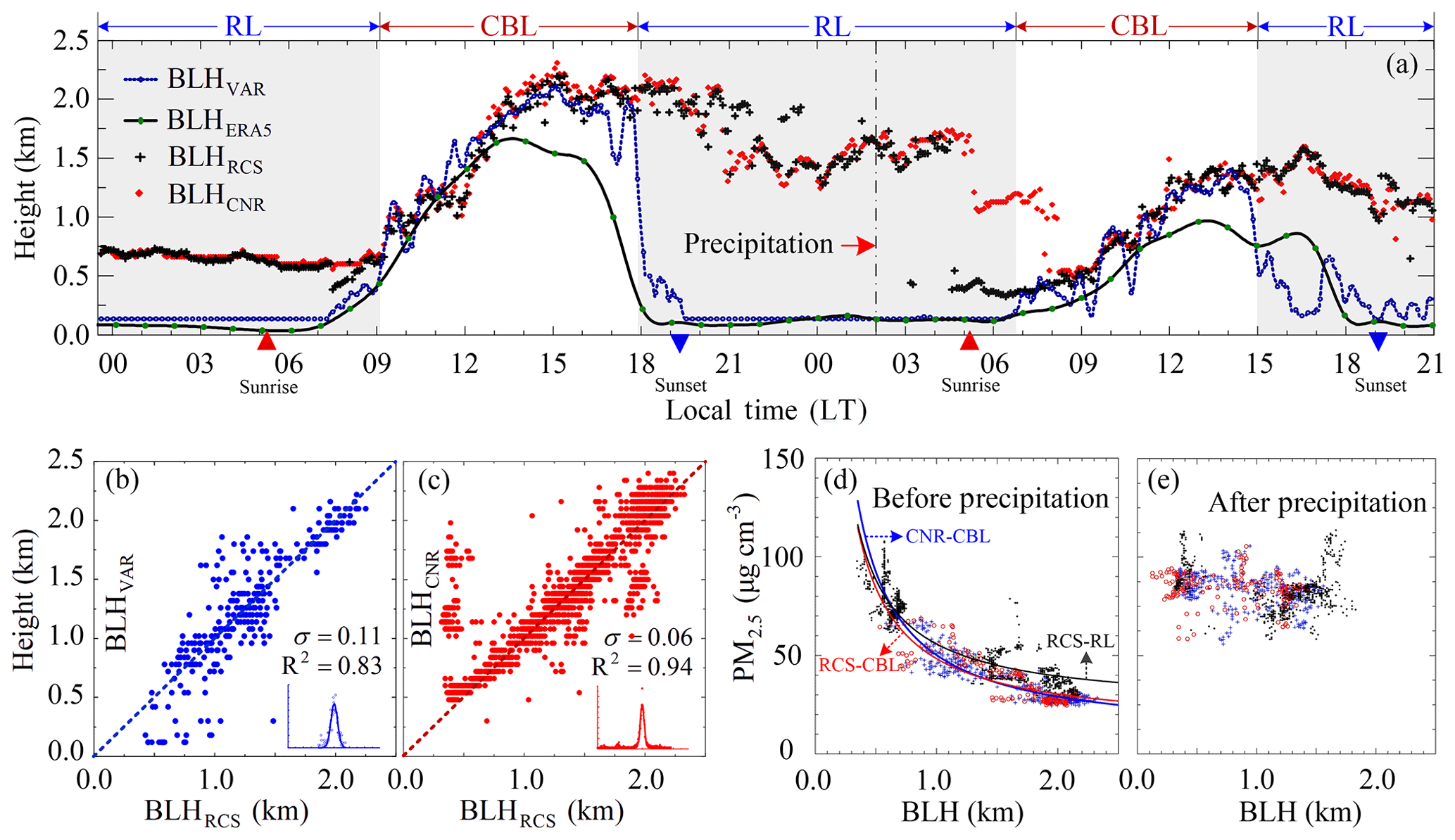
Figure 5(a) The BLH retrieval results from different methods. Scatter plots of (b) BLHVAR in CBL and (c) BLHCNR in CBL and RL versus BLHRCS for comparison. The dashed blue and dashed red lines indicate x=y. The BLH differences are plotted in right bottom in (b) and (c). The blue and red solid lines represent the corresponding Gauss fitting. R2 represents the coefficient of determination and σ represents the standard deviation of Gauss fitting. (d) The scatter plot of BLH and PM2.5 before precipitation. Red circles indicate BLHVAR in CBL, while blue plus signs indicate BLHRCS in CBL and black dots indicate BLHRCS in RL. The solid lines represent the corresponding inverse fit. (e) Same as (d) but without inverse fitting after precipitation.
Table 2The correlations between BLH and PM2.5 and the inverse fitting results.
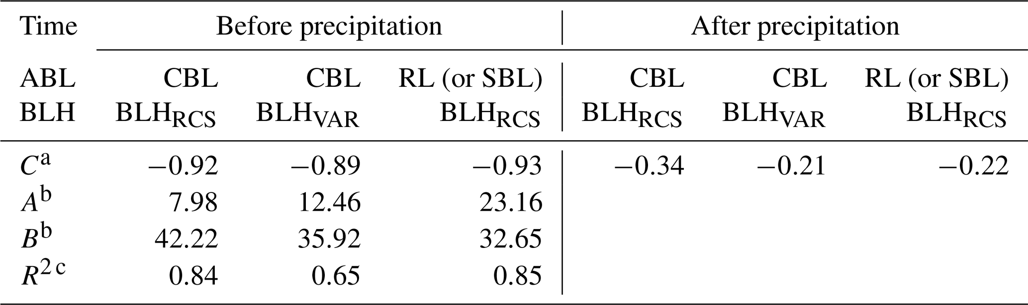
a C: correlation coefficients.
b A∕B: the parameters of the inverse fitting formula
PM.
c R2: coefficient of determination of the inverse fitting.
Figure 5d and e show the relationships between PM2.5 concentration and BLH. The correlation coefficients between BLH (BLHRCS in CBL and RL (or SBL) and BLHVAR in CBL) and PM2.5 before and after precipitation in Fig. 5d and e are listed in Table 2. An obvious anti-correlation is shown before precipitation between BLH and PM2.5 concentrations in both CBL and RL (or SBL) with a correlation coefficient of . An inverse fitting formula PM is used to describe the PM2.5–BLH relationships in Fig. 5d. The resulting parameters of A, B are listed in Table 2. The nonlinear inverse function shows good performance with a coefficient of determination R2=0.84, 0.65 and 0.85. In general, these results show good responses of PM2.5 to aerosol-derived BLH (BLHRCS) evolution with larger R2 and stronger correlation than turbulence-derived BLH (BLHVAR) both before and after precipitation. In addition, as shown in Fig. 5d, the inverse function of PM2.5 to the BLHRCS and BLHVAR show good consistency in CBL. While in RL (or SBL), the inverse function of PM2.5 to the BLHRCS is quite different from that in CBL. The parameter A in the inverse fitting formula of the PM2.5–BLH relationship for BLHRCS in RL (SL) is triple (twice) as large as that for BLHRCS (BLHVAR) in CBL, as listed in Table 2, while the parameter B has similar values. This difference of parameter A represents a higher PM2.5 concentration in RL (or SBL). After precipitation, as shown in Fig. 5e and Table 2, there are relatively weak anti-correlations of −0.34, −0.21 and −0.22, respectively. The relationships between BLH and PM2.5 are changed after precipitation. Recently, Geiß et al. (2017) investigated correlations between BLH and concentrations of pollutants (PM10, O3, NOx). They found that the correlations of BLH with PM10 were quite different for different sites without showing a clear pattern. In addition, the reflection and absorption of the incoming solar radiation by the clouds on 2 June 2018 could also affect the diffusion of aerosols. Therefore, BLH with different retrieval methods, pollutant sources and meteorological conditions should be considered in air quality prediction models.
4.4 Aerosol–cloud–ABL interaction
Moreover, the ABL in the cloudy conditions on 2 June grows slower with lower BLH than that in the fair weather conditions on 1 June, as shown in Fig. 5a. The maximum BLH on 2 June is about 1.7 km high while the maximum BLH on 1 June is about 2.3 km high. In addition, the RL tops become lower when the cloud layer occurs around 4 km altitude on 2 June. These phenomena may be in relation to the aerosol–cloud–ABL interaction. There are several transport aerosol layers above ABL, as shown in Fig. 3a. These transport aerosol layers may act as the cloud condensation nuclei during the cloud formation between ∼3 and ∼5 km on 2 June. The clouds play important roles in the Earth's energy budget. As more incoming solar radiation is reflected and absorbed by clouds, less energy enters the ABL, resulting in weaker CBL development and lower BLH on 2 June than on 1 June. In addition, the weaker convection may lead to the higher aerosol concentration in the ABL on 2 June, as shown in Fig. 3a and b. These results hinted at a strong aerosol–cloud–ABL interaction during the ABL evolution.
A compact integrated lidar system that integrates both DDL and CDWL is demonstrated. The DDL incorporated a fibre laser at 1.5 µm and an up-conversion detector. The design of this lidar makes it more eye-safe than traditional lidar using lasers of 355, 532 and 1064 nm. All-fibre configuration is realised to guarantee the high optical coupling efficiency and robust stability. Two lidar systems use only one set of instruments comprised of a laser source, optical collimator and control system. Thus, this integrated lidar can make simultaneous measurements of aerosol density, vertical wind and clouds with high spatial and temporal resolution.
The BLH values derived from aerosol and turbulence are determined from 45 h of continuous measurements. Two methods of HWCT and variance are employed in BLH determination, respectively. The BLH retrieved from different methods are comparable to each other and the RL tops are comparable as well. The standard deviation between aerosol-derived BLH from DDL and CDWL is 0.06 km. The BLH derived from vertical wind is comparable with BLH from ERA5 reanalysis data and also has a larger BLH than ERA5 due to different retrieval methods to those in other studies (Seidel et al., 2010). During the evolution of the ABL, the clouds suppress the growth of the ABL, leading to aerosol increase in the ABL. The variations in PM2.5 and BLH before and after a precipitation event in clouds are analysed in different ABL categories by adopting different methods. There is a strong inverse relation between BLH and PM2.5 in both CBL and RL∕SBL before a precipitation. However, the relationship is relatively weak after the precipitation. In addition, there is a good response of PM2.5 to aerosol-derived BLH evolution with larger R2 and stronger correlation than turbulence-derived BLH both before and after the precipitation.
The reasons for the differences in the relationships between BLH and PM2.5 may result from both cloud effect and pollutant sources and not just from the precipitation. This required more data based on different instruments, such as horizontal wind field (Shangguan et al., 2017), temperature profiles (Mattis et al., 2002), and the depolarisation ratio of aerosol (Qiu et al., 2017) and pollutant components in the ABL. To probe the mechanism of the BLH–PM2.5 relations under different conditions, such as before and after the precipitation, not only these observations but also model simulations are needed in further studies. The application of such an integrated lidar in this research will contribute to our understanding of the ABL and aerosol–cloud–precipitation interactions, and thus improve our ability to make weather forecasts and air quality predictions in future.
The ERA5 data sets are publicly available from ECMWF website at https://www.ecmwf.int/en/forecasts/datasets/reanalysis-datasets/era5 (last access: 20 May 2019). Lidar and meteorological data can be downloaded from http://www.lidar.cn/datashare/Wang_et_al_2018c.rar (last access: 20 May 2019).
Besides BLH, RL top is also important in model validation and parameterisation development. A simple method to retrieve RL top from RCS, CNR and variance of vertical velocity profiles is proposed. In order to reduce the interference from noise, the RL top is determined with a temporal resolution of 5 min. Dominant aerosol layer tops are easy to identify at around 2 km altitude, as shown in Fig. 3. Thus, the aerosol layer tops are limited between 1 and 2.5 km altitude range. A threshold method is suitable for RCS and CNR profiles. For this observation, the threshold is set to be 5×10¹⁰ for the RCS profile (1×10¹⁰ for resolution of 1 min as shown in Fig. 3a) and −30 dB for the CNR profile. For profiles of variance of vertical velocity, the aerosol layer is identified as the altitudes under the minimum altitude where invalid data exist, e.g. ∼1.6 km in Fig. 2c. If the difference between aerosol layer top and BLH is larger than a given threshold, e.g. 0.3 km in current study, the aerosol layer top is identified as RL top. It should be noted that all the values of threshold used here may vary at different places for different lidar. These values may be only suitable for during this observation.
CW and MJ contributed equally to this work. HX and XD conceived of and designed the study. CW, YW and TW performed the lidar experiment observations. XS performed the meteorological and particulate matter observations. CY downloaded and analysed the ERA5 data. MJ and CW carried out the data analysis and prepared the figures, with comments from the other co-authors. CW, MJ, HX and XX interpreted the data. CW, MJ and HX wrote the manuscript. All authors contributed to discussion and interpretation.
The authors declare that they have no conflict of interest.
We acknowledge the use of ERA5 data sets from ECMWF website at https://www.ecmwf.int/en/forecasts/datasets/reanalysis-datasets/era5 (last access: 20 May 2019). We would like to thank Matthias Wiegner for his helpful suggestions. We are grateful to Shengfu Lin, Mingjia Shangguan and Jiawei Qiu for their valuable discussions.
This paper was edited by Laura Bianco and reviewed by three anonymous referees.
Baars, H., Ansmann, A., Engelmann, R., and Althausen, D.: Continuous monitoring of the boundary-layer top with lidar, Atmos. Chem. Phys., 8, 7281–7296, https://doi.org/10.5194/acp-8-7281-2008, 2008.
Bonin, T. A., Carroll, B. J., Hardesty, R. M., Brewer, W. A., Hajny, K., Salmon, O. E., and Shepson, P. B.: Doppler Lidar Observations of the Mixing Height in Indianapolis Using an Automated Composite Fuzzy Logic Approach, J. Atmos. Ocean. Tech., 35, 473–490, https://doi.org/10.1175/jtech-d-17-0159.1, 2018.
Brooks, I. M.: Finding Boundary Layer Top: Application of a Wavelet Covariance Transform to Lidar Backscatter Profiles, J. Atmos. Ocean. Tech., 20, 1092–1105, https://doi.org/10.1175/1520-0426(2003)020<1092:fbltao>2.0.co;2, 2003.
Brunekreef, B. and Holgate, S. T.: Air pollution and health, The Lancet, 360, 1233–1242, https://doi.org/10.1016/s0140-6736(02)11274-8, 2002.
Campbell, J. R., Hlavka, D. L., Welton, E. J., Flynn, C. J., Turner, D. D., Spinhirne, J. D., Scott, V. S., and Hwang, I. H.: Full-time, eye-safe cloud and aerosol lidar observation at atmospheric radiation measurement program sites: Instruments and data processing, J. Atmos. Ocean. Tech., 19, 431–442, https://doi.org/10.1175/1520-0426(2002)019<0431:Ftesca>2.0.Co;2, 2002.
Chan, C. K. and Yao, X.: Air pollution in mega cities in China, Atmos. Environ., 42, 1–42, https://doi.org/10.1016/j.atmosenv.2007.09.003, 2008.
Chen, Y., An, J. L., Sun, Y. L., Wang, X. Q., Qu, Y., Zhang, J. W., Wang, Z. F., and Duan, J.: Nocturnal Low-level Winds and Their Impacts on Particulate Matter over the Beijing Area, Adv. Atmos. Sci., 35, 1455–1468, https://doi.org/10.1007/s00376-018-8022-9, 2018.
China Meteorological Administration: Observation and forecasting levels of haze, QX/T 113–2010, China Meteorological Press, Beijing, China, 8, available at: http://www.cma.gov.cn/root7/auto13139/201612/t20161213_350244.html, 2010.
Cohen, A. J., Brauer, M., Burnett, R., Anderson, H. R., Frostad, J., Estep, K., Balakrishnan, K., Brunekreef, B., Dandona, L., Dandona, R., Feigin, V., Freedman, G., Hubbell, B., Jobling, A., Kan, H., Knibbs, L., Liu, Y., Martin, R., Morawska, L., Pope, C. A., Shin, H., Straif, K., Shaddick, G., Thomas, M., van Dingenen, R., van Donkelaar, A., Vos, T., Murray, C. J. L., and Forouzanfar, M. H.: Estimates and 25-year trends of the global burden of disease attributable to ambient air pollution: an analysis of data from the Global Burden of Diseases Study 2015, The Lancet, 389, 1907–1918, https://doi.org/10.1016/s0140-6736(17)30505-6, 2017.
Collaud Coen, M., Praz, C., Haefele, A., Ruffieux, D., Kaufmann, P., and Calpini, B.: Determination and climatology of the planetary boundary layer height above the Swiss plateau by in situ and remote sensing measurements as well as by the COSMO-2 model, Atmos. Chem. Phys., 14, 13205–13221, https://doi.org/10.5194/acp-14-13205-2014, 2014.
Du, C., Liu, S., Yu, X., Li, X., Chen, C., Peng, Y., Dong, Y., Dong, Z., and Wang, F.: Urban Boundary Layer Height Characteristics and Relationship with Particulate Matter Mass Concentrations in Xi'an, Central China, Aerosol Air Qual. Res., 13, 1598–1607, https://doi.org/10.4209/aaqr.2012.10.0274, 2013.
ECMWF: PART IV: PHYSICAL PROCESSES, in: IFS Documentation CY43R3, IFS Documentation, ECMWF, Shinfield Park, Reading, RG2 9AX, England, 221, 2017.
Geiß, A., Wiegner, M., Bonn, B., Schäfer, K., Forkel, R., von Schneidemesser, E., Münkel, C., Chan, K. L., and Nothard, R.: Mixing layer height as an indicator for urban air quality?, Atmos. Meas. Tech., 10, 2969–2988, https://doi.org/10.5194/amt-10-2969-2017, 2017.
Godin, S., Mégie, G., and Pelon, J.: Systematic lidar measurements of the stratospheric ozone vertical distribution, Geophys. Res. Lett., 16, 547–550, https://doi.org/10.1029/GL016i006p00547, 1989.
Guo, J., Miao, Y., Zhang, Y., Liu, H., Li, Z., Zhang, W., He, J., Lou, M., Yan, Y., Bian, L., and Zhai, P.: The climatology of planetary boundary layer height in China derived from radiosonde and reanalysis data, Atmos. Chem. Phys., 16, 13309–13319, https://doi.org/10.5194/acp-16-13309-2016, 2016.
He, Q. S., Li, C. C., Mao, J. T., Lau, A. K. H., and Chu, D. A.: Analysis of aerosol vertical distribution and variability in Hong Kong, J. Geophys. Res.-Atmos., 113, D14211, https://doi.org/10.1029/2008jd009778, 2008.
Hersbach, H. and Dee, D.: ERA5 reanalysis is in production, Shinfield Park, Reading, Berkshire RG2 9AX, UK, 7, 2016.
Huang, M., Gao, Z., Miao, S., Chen, F., LeMone, M. A., Li, J., Hu, F., and Wang, L.: Estimate of Boundary-Layer Depth Over Beijing, China, Using Doppler Lidar Data During SURF-2015, Bound.-Lay. Meteorol., 162, 503–522, https://doi.org/10.1007/s10546-016-0205-2, 2016.
Huang, R. J., Zhang, Y., Bozzetti, C., Ho, K. F., Cao, J. J., Han, Y., Daellenbach, K. R., Slowik, J. G., Platt, S. M., Canonaco, F., Zotter, P., Wolf, R., Pieber, S. M., Bruns, E. A., Crippa, M., Ciarelli, G., Piazzalunga, A., Schwikowski, M., Abbaszade, G., Schnelle-Kreis, J., Zimmermann, R., An, Z., Szidat, S., Baltensperger, U., El Haddad, I., and Prevot, A. S.: High secondary aerosol contribution to particulate pollution during haze events in China, Nature, 514, 218–222, https://doi.org/10.1038/nature13774, 2014.
Kampa, M. and Castanas, E.: Human health effects of air pollution, Environ. Pollut., 151, 362–367, https://doi.org/10.1016/j.envpol.2007.06.012, 2008.
Korhonen, K., Giannakaki, E., Mielonen, T., Pfüller, A., Laakso, L., Vakkari, V., Baars, H., Engelmann, R., Beukes, J. P., Van Zyl, P. G., Ramandh, A., Ntsangwane, L., Josipovic, M., Tiitta, P., Fourie, G., Ngwana, I., Chiloane, K., and Komppula, M.: Atmospheric boundary layer top height in South Africa: measurements with lidar and radiosonde compared to three atmospheric models, Atmos. Chem. Phys., 14, 4263–4278, https://doi.org/10.5194/acp-14-4263-2014, 2014.
Large, W. G., Mcwilliams, J. C., and Doney, S. C.: Oceanic Vertical Mixing - a Review and a Model with a Nonlocal Boundary-Layer Parameterization, Rev. Geophys., 32, 363–403, https://doi.org/10.1029/94rg01872, 1994.
Li, H., Yang, Y., Hu, X.-M., Huang, Z., Wang, G., Zhang, B., and Zhang, T.: Evaluation of retrieval methods of daytime convective boundary layer height based on lidar data, J. Geophys. Res.-Atmos., 122, 4578–4593, https://doi.org/10.1002/2016jd025620, 2017a.
Li, H., Yang, Y., Hu, X. M., Huang, Z. W., Wang, G. Y., and Zhang, B. D.: Application of Convective Condensation Level Limiter in Convective Boundary Layer Height Retrieval Based on Lidar Data, Atmosphere-Basel, 8, 79, https://doi.org/10.3390/Atmos8040079, 2017b.
Li, J., Li, C., Zhao, C., and Su, T.: Changes in surface aerosol extinction trends over China during 1980–2013 inferred from quality-controlled visibility data, Geophys. Res. Lett., 43, 8713–8719, https://doi.org/10.1002/2016gl070201, 2016.
Li, Z., Guo, J., Ding, A., Liao, H., Liu, J., Sun, Y., Wang, T., Xue, H., Zhang, H., and Zhu, B.: Aerosol and boundary-layer interactions and impact on air quality, Natl. Sci. Rev., 4, 810–833, https://doi.org/10.1093/nsr/nwx117, 2017.
Manninen, A. J., Marke, T., Tuononen, M., and O'Connor, E. J.: Atmospheric Boundary Layer Classification With Doppler Lidar, J. Geophys. Res.-Atmos., 123, 8172–8189, https://doi.org/10.1029/2017JD028169, 2018.
Mattis, I., Ansmann, A., Althausen, D., Jaenisch, V., Wandinger, U., Müller, D., Arshinov, Y. F., Bobrovnikov, S. M., and Serikov, I. B.: Relative-humidity profiling in the troposphere with a Raman lidar, Appl. Optics, 41, 6451, https://doi.org/10.1364/ao.41.006451, 2002.
Miao, Y., Liu, S., Guo, J., Huang, S., Yan, Y., and Lou, M.: Unraveling the relationships between boundary layer height and PM2.5 pollution in China based on four-year radiosonde measurements, Environ. Pollut., 243, 1186–1195, https://doi.org/10.1016/j.envpol.2018.09.070, 2018.
Murray, E. R. and van der Laan, J. E.: Remote measurement of ethylene using a CO2 differential-absorption lidar, Appl. Optics, 17, 814–817, https://doi.org/10.1364/AO.17.000814, 1978.
Petaja, T., Jarvi, L., Kerminen, V. M., Ding, A. J., Sun, J. N., Nie, W., Kujansuu, J., Virkkula, A., Yang, X. Q., Fu, C. B., Zilitinkevich, S., and Kulmala, M.: Enhanced air pollution via aerosol-boundary layer feedback in China, Sci. Rep.-UK, 6, 6, https://doi.org/10.1038/srep18998, 2016.
Qiu, J., Xia, H., Shangguan, M., Dou, X., Li, M., Wang, C., Shang, X., Lin, S., and Liu, J.: Micro-pulse polarization lidar at 1.5 µm using a single superconducting nanowire single-photon detector, Opt. Lett., 42, 4454–4457, https://doi.org/10.1364/OL.42.004454, 2017.
Reitebuch, O.: Wind Lidar for Atmospheric Research, in: Atmospheric Physics, edited by: Schumann, U., Research Topics in Aerospace, Springer, Berlin, Heidelberg, 487–507, 2012.
Renaut, D., Pourny, J. C., and Capitini, R.: Daytime Raman-lidar measurements of water vapor, Opt. Lett., 5, 233–235, https://doi.org/10.1364/ol.5.000233, 1980.
Sawyer, V. and Li, Z.: Detection, variations and intercomparison of the planetary boundary layer depth from radiosonde, lidar and infrared spectrometer, Atmos. Environ., 79, 518–528, https://doi.org/10.1016/j.atmosenv.2013.07.019, 2013.
Seibert, P.: Review and intercomparison of operational methods for the determination of the mixing height, Atmos. Environ., 34, 1001–1027, https://doi.org/10.1016/s1352-2310(99)00349-0, 2000.
Seidel, D. J., Ao, C. O., and Li, K.: Estimating climatological planetary boundary layer heights from radiosonde observations: Comparison of methods and uncertainty analysis, J. Geophys. Res.-Atmos., 115, D16113, https://doi.org/10.1029/2009jd013680, 2010.
Seidel, D. J., Zhang, Y. H., Beljaars, A., Golaz, J. C., Jacobson, A. R., and Medeiros, B.: Climatology of the planetary boundary layer over the continental United States and Europe, J. Geophys. Res.-Atmos., 117, D17106, https://doi.org/10.1029/2012jd018143, 2012.
Shang, X., Xia, H., Dou, X., Shangguan, M., Li, M., and Wang, C.: Adaptive inversion algorithm for 1.5 µm visibility lidar incorporating in situ Angstrom wavelength exponent, Opt. Commun., 418, 129–134, https://doi.org/10.1016/j.optcom.2018.03.009, 2018.
Shangguan, M., Xia, H., Wang, C., Qiu, J., Lin, S., Dou, X., Zhang, Q., and Pan, J. W.: Dual-frequency Doppler lidar for wind detection with a superconducting nanowire single-photon detector, Opt. Lett., 42, 3541–3544, https://doi.org/10.1364/OL.42.003541, 2017.
Song, C., Wu, L., Xie, Y., He, J., Chen, X., Wang, T., Lin, Y., Jin, T., Wang, A., Liu, Y., Dai, Q., Liu, B., Wang, Y. N., and Mao, H.: Air pollution in China: Status and spatiotemporal variations, Environ. Pollut., 227, 334–347, https://doi.org/10.1016/j.envpol.2017.04.075, 2017.
Stull, R. B.: An Introduction to Boundary Layer Meteorology, Kluwer Academic Publishers, Dordrecht, the Netherlands, 1988.
Su, T., Li, Z., and Kahn, R.: Relationships between the planetary boundary layer height and surface pollutants derived from lidar observations over China: regional pattern and influencing factors, Atmos. Chem. Phys., 18, 15921–15935, https://doi.org/10.5194/acp-18-15921-2018, 2018.
Vogelezang, D. H. P. and Holtslag, A. A. M.: Evaluation and model impacts of alternative boundary-layer height formulations, Bound.-Lay. Meteorol., 81, 245–269, https://doi.org/10.1007/bf02430331, 1996.
Wang, C., Xia, H., Shangguan, M., Wu, Y., Wang, L., Zhao, L., Qiu, J., and Zhang, R.: 1.5 µm polarization coherent lidar incorporating time-division multiplexing, Opt. Express, 25, 20663–20674, https://doi.org/10.1364/OE.25.020663, 2017.
Wei, W., Zhang, H., Wu, B., Huang, Y., Cai, X., Song, Y., and Li, J.: Intermittent turbulence contributes to vertical dispersion of PM2.5 in the North China Plain: cases from Tianjin, Atmos. Chem. Phys., 18, 12953–12967, https://doi.org/10.5194/acp-18-12953-2018, 2018.
Xia, H., Sun, D., Yang, Y., Shen, F., Dong, J., and Kobayashi, T.: Fabry-Perot interferometer based Mie Doppler lidar for low tropospheric wind observation, Appl. Optics, 46, 7120, https://doi.org/10.1364/ao.46.007120, 2007.
Xia, H., Shentu, G., Shangguan, M., Xia, X., Jia, X., Wang, C., Zhang, J., Pelc, J. S., Fejer, M. M., Zhang, Q., Dou, X., and Pan, J. W.: Long-range micro-pulse aerosol lidar at 1.5 µm with an upconversion single-photon detector, Opt. Lett., 40, 1579–1582, https://doi.org/10.1364/OL.40.001579, 2015.
Yang, T., Wang, Z., Zhang, W., Gbaguidi, A., Sugimoto, N., Wang, X., Matsui, I., and Sun, Y.: Technical note: Boundary layer height determination from lidar for improving air pollution episode modeling: development of new algorithm and evaluation, Atmos. Chem. Phys., 17, 6215–6225, https://doi.org/10.5194/acp-17-6215-2017, 2017.
Zhang, Q., He, K., and Huo, H.: Policy: Cleaning China's air, Nature, 484, 161–162, https://doi.org/10.1038/484161a, 2012.