the Creative Commons Attribution 4.0 License.
the Creative Commons Attribution 4.0 License.
 | 21 Jan 2019
Assessing the impact of different liquid water permittivity models on the fit between model and observations
Katrin Lonitz
Alan J. Geer
Permittivity models for microwave frequencies of liquid water below 0 ∘C (supercooled liquid water) are poorly constrained due to limited laboratory experiments and observations, especially for high microwave frequencies. This uncertainty translates directly into errors in retrieved liquid water paths of up to 80 %. This study investigates the effect of different liquid water permittivity models on simulated brightness temperatures by using the all-sky assimilation framework of the Integrated Forecast System. Here, a model configuration with an improved representation of supercooled liquid water has been used. The comparison of five different permittivity models with the current one shows a small mean reduction in simulated brightness temperatures of at most 0.15 K at 92 GHz on a global monthly scale. During austral winter, differences occur more prominently in the storm tracks of the Southern Hemisphere and in the intertropical convergence zone with values of around 0.5 to 1.5 K. Compared to the default Liebe (1989) approach, the permittivity models of Stogryn et al. (1995), Rosenkranz (2015) and Turner et al. (2016) all improve fits between observations and all-sky brightness temperatures simulated by the Integrated Forecast System. In cycling data assimilation these newer models also give small improvements in short-range humidity forecasts when measured against independent observations. Of the three best-performing models, the Stogryn et al. (1995) model is not quite as beneficial as the other two, except at 183 GHz. At this frequency, Rosenkranz (2015) and Turner et al. (2016) look worse because they expose a scattering-related forward model bias in frontal regions. Overall, Rosenkranz (2015) is favoured due to its validity up to 1 THz, which will support future submillimetre missions.
- Article
(15584 KB) - Full-text XML
- BibTeX
- EndNote


The occurrence of liquid water for temperatures below 0 ∘C (supercooled liquid water) is typical for clouds in the higher latitudes (e.g. in frontal systems and cold-air outbreak regions). Inside clouds, liquid water can exist down to −40 ∘C (Heymsfield et al., 1991). Due to a lack of laboratory experiments and observations the constraint on absorption properties of supercooled liquid water is poor. More precisely, the permittivity (or dielectric constant) of liquid water, which is one of the key factors determining the absorption in the microwave band, is poorly known for these low temperatures and, hence, existing liquid water permittivity models differ substantially. Recently, two new liquid water permittivity models by Rosenkranz (2015) and Turner et al. (2016) have been published. Both models are based partly on findings by Kneifel et al. (2014), who compared existing permittivity models (Ellison, 2007; Stogryn et al., 1995) with new observations from ground-based microwave radiometers between 31 and 225 GHz for clouds from 0 to −33 ∘C. Kneifel et al. (2014) found that the different liquid water permittivity models agree fairly well with each other between 0 and −15 ∘C, but differ by 25 % and more at lower temperatures (i.e. for supercooled liquid water), especially for frequencies higher than 35 GHz.
Liquid water permittivity models are usually compared with observations undertaken at certain locations or with laboratory results. In this study we quantify the global and local impacts of the different permittivity models for pure liquid water in the context of the assimilation of microwave imager observations that are sensitive to clouds, humidity and precipitation using the Integrated Forecast System (IFS) of the ECMWF. Since 2009, ECMWF has used an all-sky framework for the assimilation of microwave radiances (Bauer et al., 2010), which means that these observations are assimilated under clear, cloudy and precipitating conditions.
To allow a thorough study of the impact of different liquid water permittivity models for the simulation of microwave imager observations, the assimilation system and the forecast model have to have some special characteristics. First, the assimilation has to allow the simulation of observations under cloudy conditions, which is the case for microwave imager observations inside the IFS. Second, the forecast model should have skill in representing areas which are of most interest when it comes to studying the effect of absorption properties of liquid water. As shown by Kneifel et al. (2014), these are areas containing supercooled liquid water. A recent study by Forbes et al. (2016) showed, however, that one of the long-standing model biases in the shortwave radiation in the IFS is related to a lack of supercooled liquid water in cold-air outbreak regions. This bias is also well known for other numerical weather prediction (NWP) and climate models (Bodas-Salcedo et al., 2016). For this reason, a special model configuration of the IFS has been used, incorporating improvements which allow the generation of more supercooled liquid water (see Sect. 2.3).
Accurate absorption properties of cloud liquid water are needed for the construction of a reliable observation operator for microwave observations. Uncertainties, e.g. in absorption properties of cloud liquid water inside the observation operator, have, therefore, the potential to introduce systematic situation-dependent errors. For the all-sky assimilation of microwave radiances inside the IFS, the observation operator RTTOV-SCATT (Sect. 2.1) is used. It converts physical variables, e.g. humidity and temperature, from the model into observed variables, e.g. brightness temperatures. At the moment the liquid water permittivity model by Liebe (1989) is used inside RTTOV-SCATT. However, as Kneifel et al. (2014) have shown that newer permittivity models might be more suitable, especially in areas with supercooled liquid water (e.g. cold-air outbreaks), where a high uncertainty among the different permittivity models exists.
There is a great need to conduct such a “closure” study about the best choice of permittivity model for liquid water. We examine this issue using a high-quality NWP model for the first time. This approach enables the quantification of the impact of the different permittivity models globally and the comparison of the effect with other independent observations. In detail, this closure study examines the effect of six different formulations of permittivity on simulated brightness temperatures and departures, especially for areas in which clouds with supercooled liquid water prevail. First, the observation operator, the usage of data and the set-up of this study are explained. Next, the impacts on absorption and simulated brightness temperatures are shown for the different permittivity models. Eventually, the best model based on monitoring and assimilation experiments is chosen.
2.1 Observation operator RTTOV-SCATT
RTTOV-SCATT is the observation operator for the microwave radiative transfer in cloudy, precipitating and clear skies (Bauer et al., 2006) and is a component of the RTTOV package (Saunders et al., 1999). The radiative transfer equation is solved using the delta-Eddington approximation, which produces mean errors of less than 0.5 K at the targeted microwave frequencies between 10 and 200 GHz (Bauer et al., 2006). The final all-sky brightness temperature is a weighted average of the brightness temperature from a cloudy and a clear sub-column, where the weighting is done using an effective cloud fraction (Geer et al., 2009).
Generally speaking, radiation in the atmosphere can be absorbed or scattered by atmospheric particles like aerosols, atmospheric gases and hydrometeors. Which one of these processes dominates depends on the frequency, the size and shape of the particles and in the case of conducting materials like hydrometeors on the relative permittivity. We use Mie theory to compute scattering and absorption properties of cloud liquid hydrometeors which are assumed to be homogeneous.
In order to solve the radiative transfer equation the bulk optical properties of the atmosphere have to be known at each model level. Given the optical properties of a single particle, the bulk optical properties, i.e. extinction coefficient, scattering coefficient and average asymmetry parameter, can be computed by integration across a size distribution. Bulk optical properties are stored in look-up tables for different frequencies, temperatures and liquid/ice water contents for each hydrometeor type: in the IFS these are rain, snow, cloud water and cloud ice (Bauer, 2001; Geer and Baordo, 2014). For cloud droplets, scattering in the microwave regime is generally negligible and, hence, their extinction is equal to the absorption. However, for raindrops or snow, Mie scattering occurs given that the ratio between their size and the wavelength can be much larger than for cloud droplets.
The absorption of liquid clouds depends among other things on the relative permittivity of water. Permittivity is a measure of the collective motion of the molecular dipole moments under the influence of an electric field and consists of a real component and an imaginary component. How strong the permittivity is depends on frequency, pressure and temperature (and salinity, which is 0 for pure water), as illustrated later in Sect. 3. In this study, different permittivity formulations of liquid hydrometeors (e.g. cloud droplets and raindrops) are examined. The permittivity formulation inside the ocean surface emissivity model FASTEM 6 (Kazumori and English, 2015) remains unchanged.
2.2 Specifications of microwave observations
To investigate the effect of the different liquid water permittivity models, this study mainly analyses changes in simulated brightness temperature from SSMIS-F17 (Kunkee et al., 2008). As already mentioned, microwave imagers and microwave humidity sounders are assimilated under cloudy, precipitating and clear-sky (all-sky) conditions using the IFS. Currently, this includes instruments like GMI (GPM Microwave Imager), AMSR2 (Advanced Microwave Scanning Radiometer 2), MHS (Microwave Humidity Sounding), SAPHIR (Sondeur Atmospherique du Profil d'Humidite Intertropicale par Radiometrie), MWHS-2 (Micro-Wave Humidity Sounder-2) and of course SSMIS. Other microwave sensors, like AMSU-A (Advanced Microwave Sounding Unit – A) and ATMS (Advanced Technology Microwave Sounder) are still assimilated in clear-sky conditions. Alongside this, a suite of other data are assimilated, e.g. radiance from hyperspectral infrared sounders, atmospheric motion vectors, radiosondes and aircraft data.
In the all-sky system, microwave imager observations are only assimilated over ocean, whereas microwave humidity sounder observations at 183 GHz are assimilated over ocean and land. For frequencies 186 ± 6 GHz and below, data are restricted to 60∘ S and 60∘ N and exclude ocean areas with sea ice. Higher peaking microwave humidity sounding channels are assimilated over ocean and land globally, but also above sea ice. Areas with high orography are also excluded for microwave humidity sounder observations. Furthermore, microwave imager data are averaged (or “superobbed”) to about 80 km×80 km boxes in order to match the effective resolution of cloudy and precipitating systems inside the forecast model. Additionally, microwave imager data are screened in some areas because of systematic model biases, e.g. in cold-air outbreak regions (Lonitz and Geer, 2015). The data are also thinned to about 100 km. Further details of the all-sky microwave imager assimilation at ECMWF can be found in Bauer et al. (2010) and Geer et al. (2018).
A specific observation error model was designed for the assimilation of microwave observation in all-sky conditions. Here, the observation error is based on the “symmetric” cloud amount (C37), which is an average of the observed and simulated cloud amount, represented in a cloud proxy variable from 0 to 1. For SSMIS-F17, an observation error of 1.8 K is used in clear-sky conditions (C37 < 0.02), which increases linearly up to 18 K for very cloudy locations with C37 > 0.42. The higher the observation error, the less impact the observation has on the analysis. More details can be found in Geer and Bauer (2011).
2.3 Set-up of models and experiments
2.3.1 Liquid water permittivity models
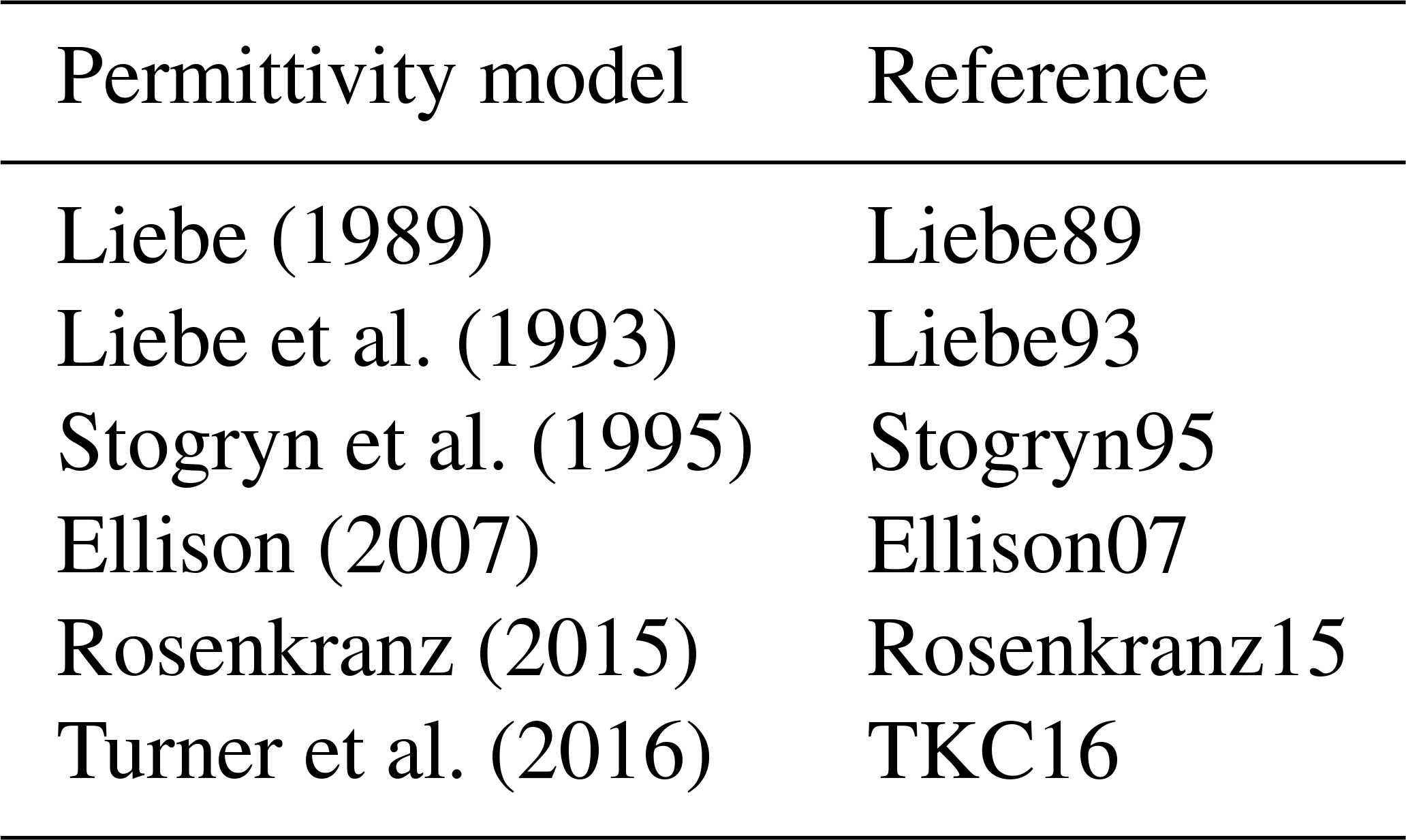
Six different permittivity models incorporated into the observation operator RTTOV-SCATT (version 11.2) have been tested in the all-sky assimilation of microwave radiances. As stated above, only the formulation of permittivity of pure liquid water clouds and rain has been altered. Table 1 lists the acronyms for the different permittivity models used in the remainder of this paper.
All liquid water permittivity models are based on laboratory data, as well as field experiments when available. These observations have been used to construct a model using a multiple Debye formulation (Debye, 1929) to describe the different forms of motion of the molecular dipole moments; e.g. reorientation and bending, also referred to as relaxation terms. The current permittivity model for liquid water, Liebe (1989), along with Liebe et al. (1993), Stogryn et al. (1995) and Turner et al. (2016), utilises a double Debye formulation, whereas Rosenkranz (2015) and Ellison (2007) apply three relaxation terms to be able to describe two modes of bending instead of just one. However, only Liebe (1989) and Liebe et al. (1993) are constructed explicitly for suspended water droplets, whereas the other models do not make special considerations or are constructed based on laboratory experiments with bulk water, for example Ellison (2007).
Liebe (1989), Liebe et al. (1993) and Rosenkranz (2015) have been constructed to be valid up to 1 THz, whereas Stogryn et al. (1995) and Turner et al. (2016) are only valid up to 500 GHz. Ellison (2007) constructed a permittivity model to be valid up to 25 THz. Therefore, his permittivity model takes two resonance terms into account, additionally to the three relaxation terms, due to the stretching of intramolecular hydrogen bonds around 4 THz and librational motions of water molecules around 11 THz. Most of the models also claim validity below 0 ∘C (Ellison, 2007), even though observations for supercooled liquid water are rare. Only the two most recent permittivity models for microwave frequencies Rosenkranz (2015) and Turner et al. (2016), incorporated a new observational data set by Kneifel et al. (2014) that measured at temperatures well below 0 ∘C. Hence, Rosenkranz (2015) and Turner et al. (2016) are believed to be more accurate at temperatures below 0 ∘C than earlier models from Liebe (1989), Liebe et al. (1993), Stogryn et al. (1995) and Ellison (2007). For more information about the basis and settings of the different liquid water permittivity models, the reader is advised to read through the literature listed in Table 1.
Liebe (1989)Liebe et al. (1993)Stogryn et al. (1995)Ellison (2007)Rosenkranz (2015)Turner et al. (2016)Table 1List of different liquid water permittivity models and how they are referenced within this paper.
2.3.2 Forecast model
In order to evaluate the quality of the different liquid water permittivity models, the simulated brightness temperatures are compared with the observed brightness temperatures from SSMIS-F17. Nevertheless, to make a fair comparison it is essential to use a suitable atmospheric model for which the liquid water in cloud and rain is realistically represented compared to the real world.
Until IFS cycle 43R1, convective mixed-phase clouds have been represented by a fixed global diagnostic temperature-dependent function. That means, for temperatures above 0 ∘C, cloud water was considered liquid, and below −23 ∘C cloud water was considered ice. Between 0 and −23 ∘C there existed a decreasing proportion of liquid water and ice. In reality, however, a cloud can consist completely of (supercooled) liquid water below 0 ∘C, depending on the evolution of the cloud and its environment. In IFS cycle 43R3 the lower threshold for the convective mixed phase was lowered to −38 ∘C to meet findings by Heymsfield et al. (1991) while allowing additional detrainment of rain and snow (ECMWF, 2017). In the most current IFS cycle 45R1 the model physics have been altered to allow the generation of purely supercooled liquid water for surface-driven shallow convection, whereas the mixed-phase formulation still applies for deep and congestus clouds.
In this study, a model configuration uses a modified version of the IFS cycle 43R3 with a horizontal resolution of approximately 16 km (T639 in spectral terms) and 137 vertical levels. This model configuration is based on IFS cycle 43R3 but utilises the 45R1 model physics, which allow the generation of more supercooled liquid water inside surface-driven shallow convection clouds down to −38 ∘C. This set-up allows us to study the sensitivity of the different liquid water permittivity models for temperatures well below 0 ∘C inside a NWP model, which would have not been possible before due to a lack of supercooled liquid water (Forbes et al., 2016). However, we know that not allowing the generation of purely supercooled liquid water congestus clouds or deep convection is one limitation of this formulation, which has to be addressed in the future. This model configuration is used for all monitoring and assimilation experiments. Using other set-ups of the IFS or other forecast systems may yield different results than what is seen in this study.
2.3.3 Experiments
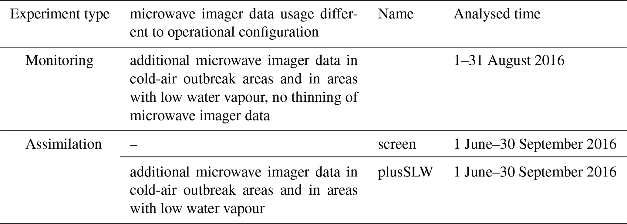
The first set of experiments are monitoring experiments, which monitor a change in first-guess departure without generating a new analysis and forecast. These experiments are used in Sects. 3 and 4. They enable the examination of the change in the simulated brightness temperature (or first guess, FG) due to a change in the observation operator only and not through subsequent changes in the analysis field that would result from a full-cycling data assimilation system. All monitoring experiments use the same parent 43R3 experiment with 45R1 model physics additionally assimilating microwave imager data in cold-air outbreak areas and in areas with a total water vapour content below 8 kg m−2 (Lonitz and Geer, 2015). Furthermore, to allow for a greater sample, no thinning of the microwave imager data has been applied as done operationally. The experiments have run from 25 July to 31 August 2016, covering times where clouds with supercooled liquid water prevail in the midlatitudes to high latitudes of the Southern Hemisphere. The analysed time frame covers 1 to 31 August 2016.
The second set of experiments allows fully cycled data assimilation and is used to evaluate the impact of the choice in liquid water permittivity model on forecast scores and fits to observations (Sect. 5). All experiments use the same set-up run using IFS cycle 43R3 with 45R1 model physics. Two assimilation experiments are carried out, one which screens cold-air outbreak areas (screen) and one which assimilates data in these regions (plusSLW). The experiments ran from 1 June to 30 September 2016. A summary of all experiment types is given in Table 2.
Table 2List of different experiment set-ups and their details, which have been run using different liquid water permittivity models.
As mentioned in Sect. 1 the largest changes from using different liquid water permittivity models are expected for high microwave frequencies (larger than 35 GHz) and in areas of supercooled liquid water clouds, as shown, for example, by Cadeddu and Turner (2011). Little impact is expected for precipitation with supercooled liquid water in these experiments. This is because supercooled drizzle does not yet exist inside the model and supercooled raindrops exist only for very few cases just below 0 ∘C (Richard Forbes, personal communication, ECMWF, 2018). Here, we investigate how the different permittivity formulations modulate absorption properties of liquid water and simulated brightness temperatures at different frequencies.
3.1 Absorption properties
Figure 1 shows how absorption varies with temperature for a liquid-water cloud with 0.1 g m−3 water content. As expected, the largest variations in absorption occur for high microwave frequencies: 92 GHz and higher (Fig. 1). The higher the frequency, the more the spread between the models can be seen for higher temperatures. Here, the largest spread can be seen for temperature below 0 ∘C (273 K). Most of the models show slightly smaller values in absorption compared to Liebe89 with two exceptions in Ellison07 for temperatures between 255 and 290 K and in Liebe93 for temperatures below 255 K, both for frequencies of 92 GHz and higher.
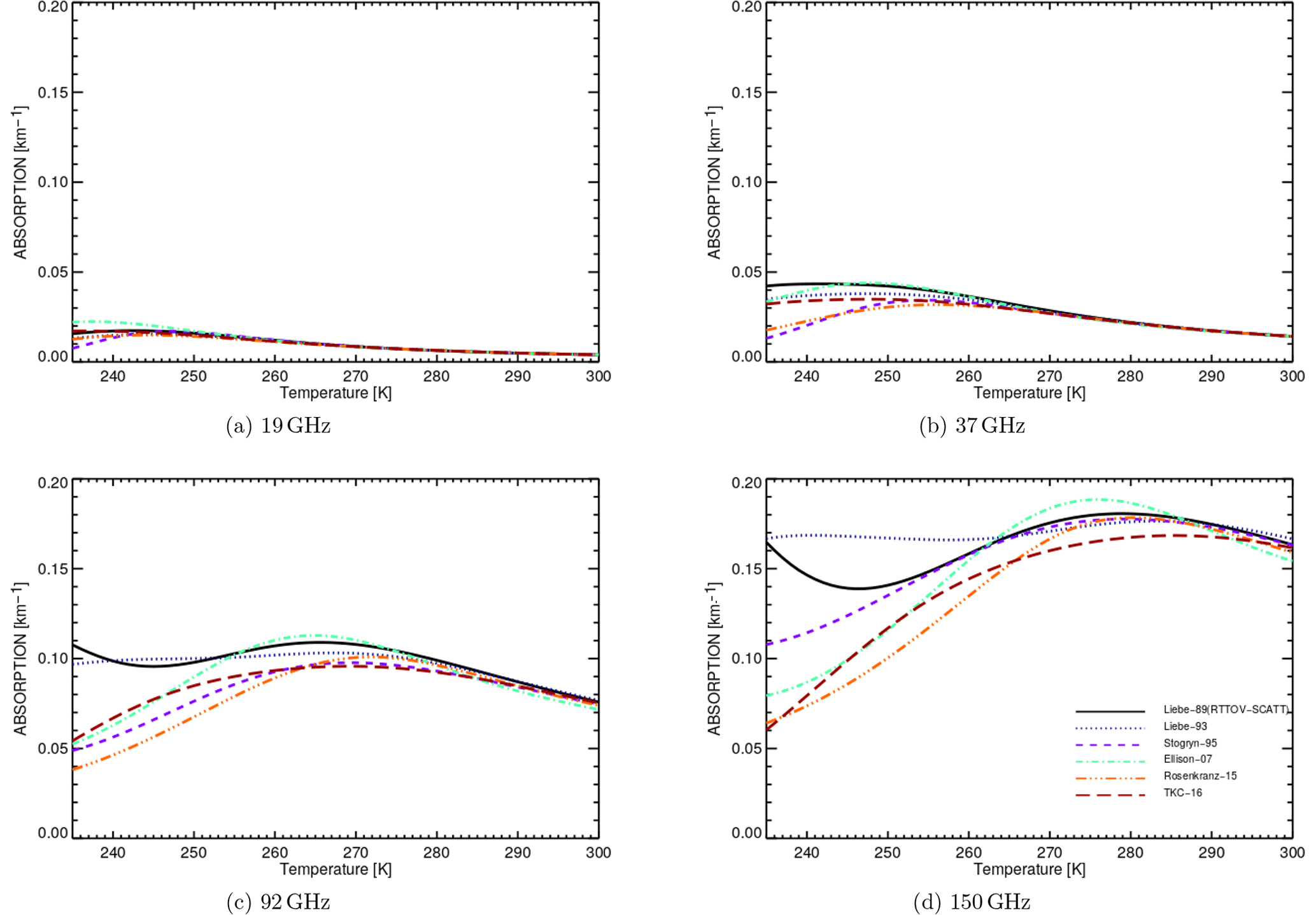
Figure 1Absorption as a function of temperature for liquid water clouds with 0.1 g m−3 water content for different microwave frequencies.
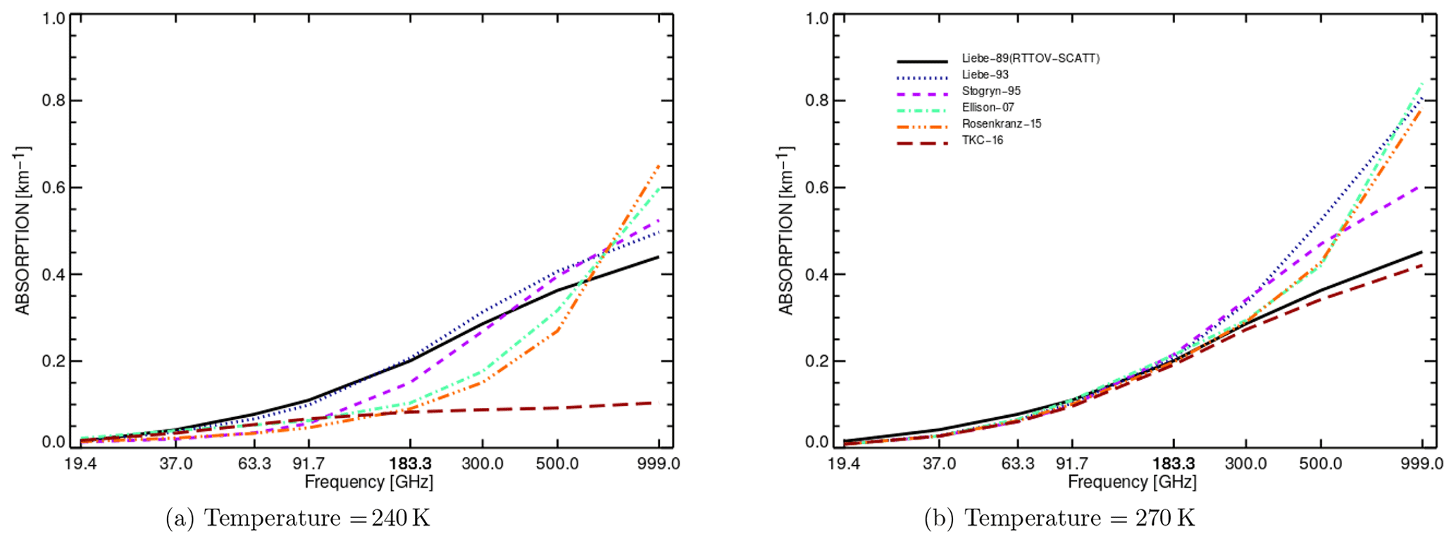
Figure 2Absorption as a function of different microwave frequencies for liquid water clouds with 0.1 g m−3 water content at temperatures of (a) T=240 K and (b) T=270 K. For the construction of these figures, absorption values have been computed at 19.4, 37, 63.3, 91.7, 183, 300, 500 and 999 GHz. Values of absorption between these frequencies are linearly interpolated.
Figure 2 shows variation with frequency for up to 1 THz. For temperatures around 0 ∘C (Fig. 2b), the absorption increases with frequency for all permittivity formulations. At 270 K all permittivity models show larger absorption values at 1 THz compared to 200 GHz, e.g. with values twice as high for TKC16 and almost 4 times higher for Rosenkranz15 (Fig. 2b). At 240 K the discrepancy between the models is even higher (Fig. 2a). Here, the two most recent permittivity models, Rosenkranz15 and TKC16, give about 50 % of the absorption compared to Liebe89 for frequencies around the 183 GHz water vapour absorption line. Quite large differences can be seen for higher frequencies above 200 GHz. The absorption given by TKC16 seems to saturate for frequencies above 92 GHz, whereas for all the other permittivity models absorption increases with frequency throughout the whole frequency spectrum. Here, Rosenkranz15 shows the largest increase with frequency, having an absorption value of about 0.65 km−1 at 1 THz (Fig. 2a). These main differences between Rosenkranz15 and TKC16 may be due to the subset of observations used to build the models, the differences in the Debye formulations or the method used to fit the absorption model coefficients. We think that the combination of a third relaxation term and fitting observations for frequencies up to 1 THz for Rosenkranz15 explains most of the differences in the higher-frequency spectrum compared to TKC16, which only uses two relaxation terms and is constructed to be valid up to 500 GHz.
3.2 Effect of liquid water permittivity models on simulated brightness temperature
Results from the monitoring experiments show that reduced absorption decreases the simulated brightness temperatures for some frequencies. This can be seen in the mean difference in simulated brightness temperatures from various monitoring experiments using permittivity models at 37 GHz, V polarised (37 v), 92 GHz, V polarised (92 v) and 150 GHz, H polarised (150 h) co-located to SSMIS-F17 observations. Table 3 gives an overview of mean differences in the Northern Hemisphere, in the tropics and in the Southern Hemisphere. Most permittivity models show a small mean reduction in brightness temperature compared to Liebe89 in all regions, but especially in the Southern Hemisphere during austral winter. The largest (but still quite small) mean deviation from Liebe89 is found in the Southern Hemisphere for TKC16 at 92 v with a mean reduction of 0.288 K in simulated brightness temperature. The smallest difference is found for Liebe93 of about 0.003 K at 150 h in the Southern Hemisphere.
Table 3Mean difference in simulated brightness temperature [K] between the newer liquid water permittivity models and the current Liebe89 for 37 v, 92 v and 150 h at locations of all selected SSMIS-F17 observations over the time period 1 to 31 August 2016 for the Northern Hemisphere (NH: 20 to 90∘ N), tropics (20∘ N to 20∘ S) and Southern Hemisphere (SH: 20 to 90∘ S).
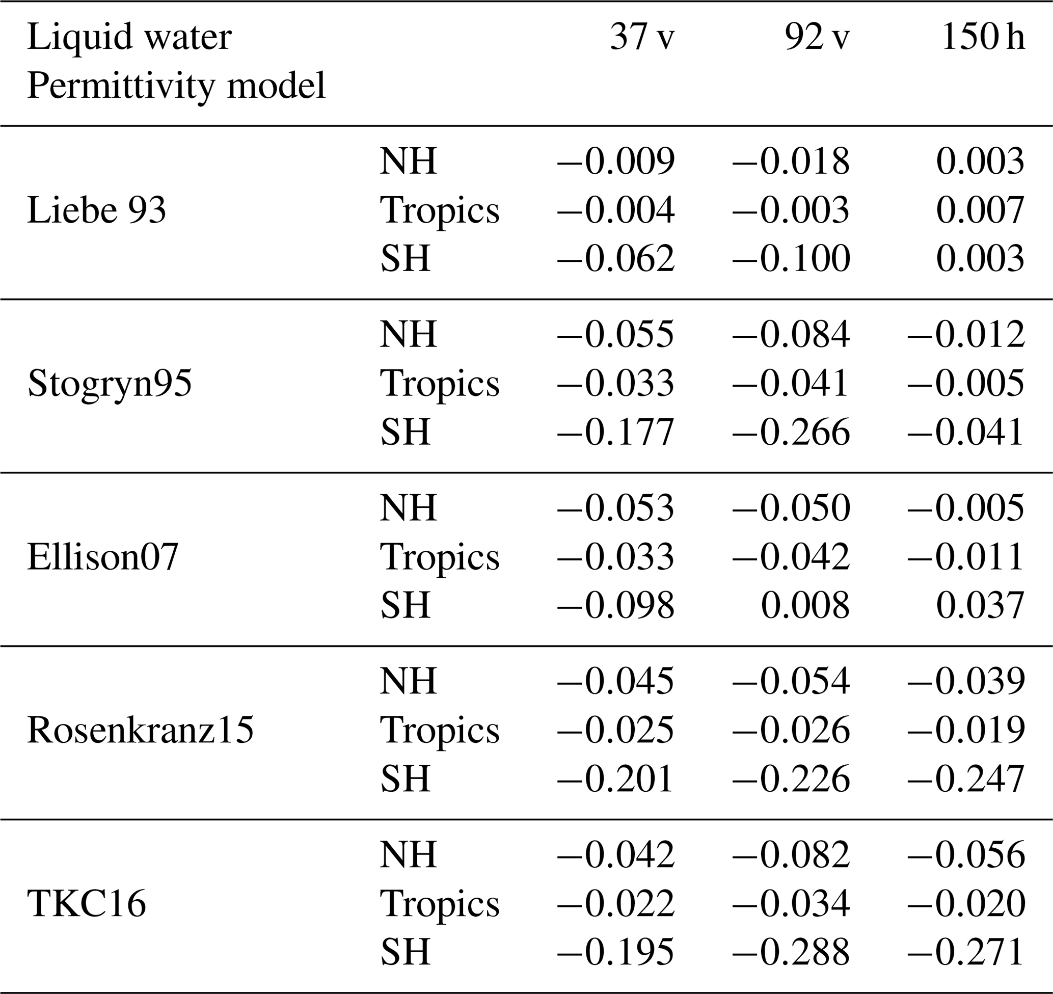
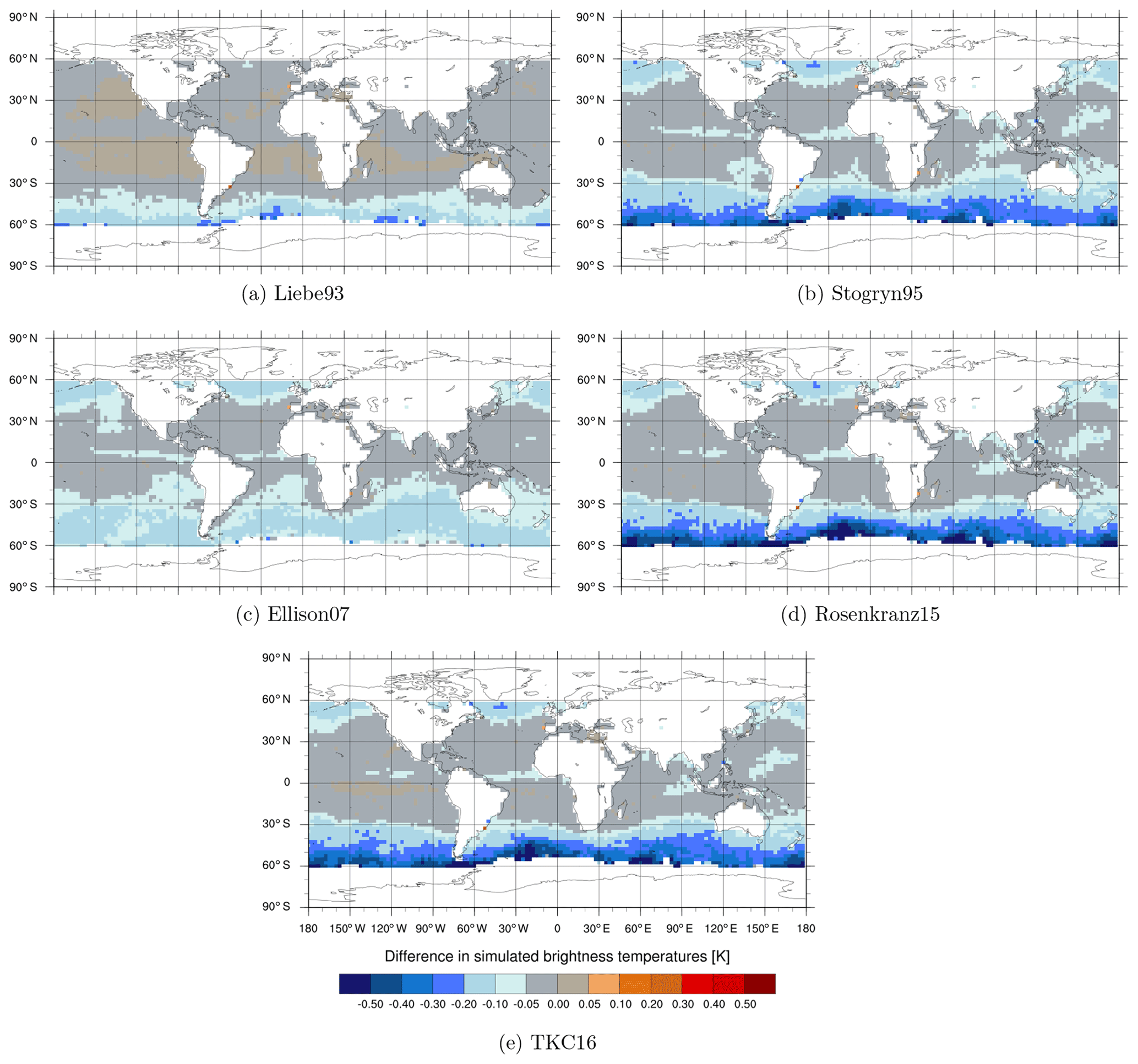
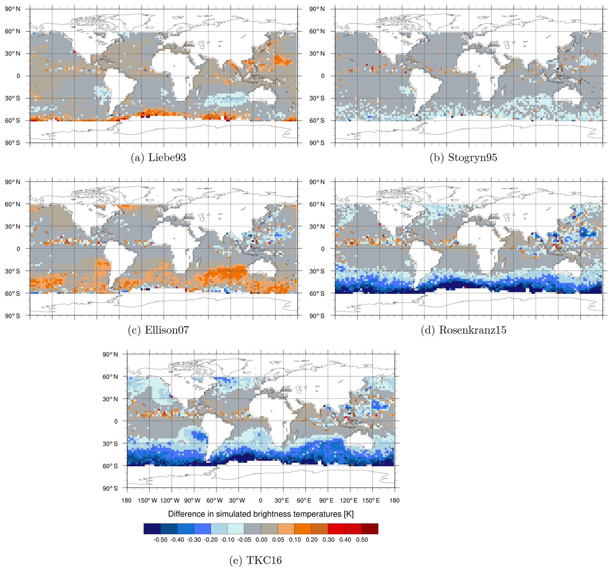
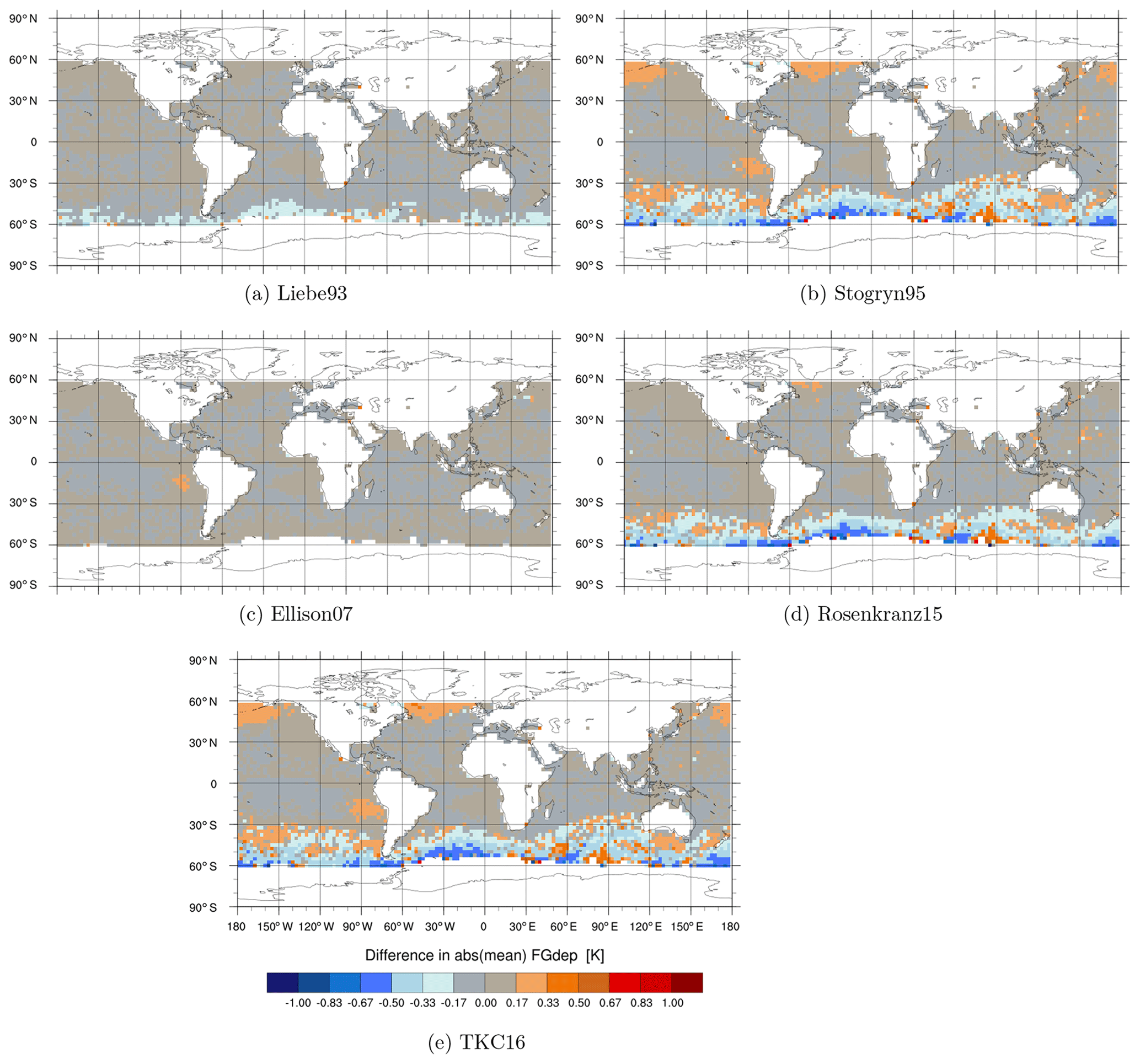
Figure 3Maps of differences in simulated brightness temperatures [K] between the newer liquid water permittivity models and the current Liebe89 for 37 v brightness temperatures co-located to corresponding SSMIS-F17 observations. Means are computed in each 2.5∘lat × 2.5∘long bin and over the time period 1 to 31 August 2016. White areas correspond to areas in which data are not assimilated, as mentioned in Sect. 2.2.
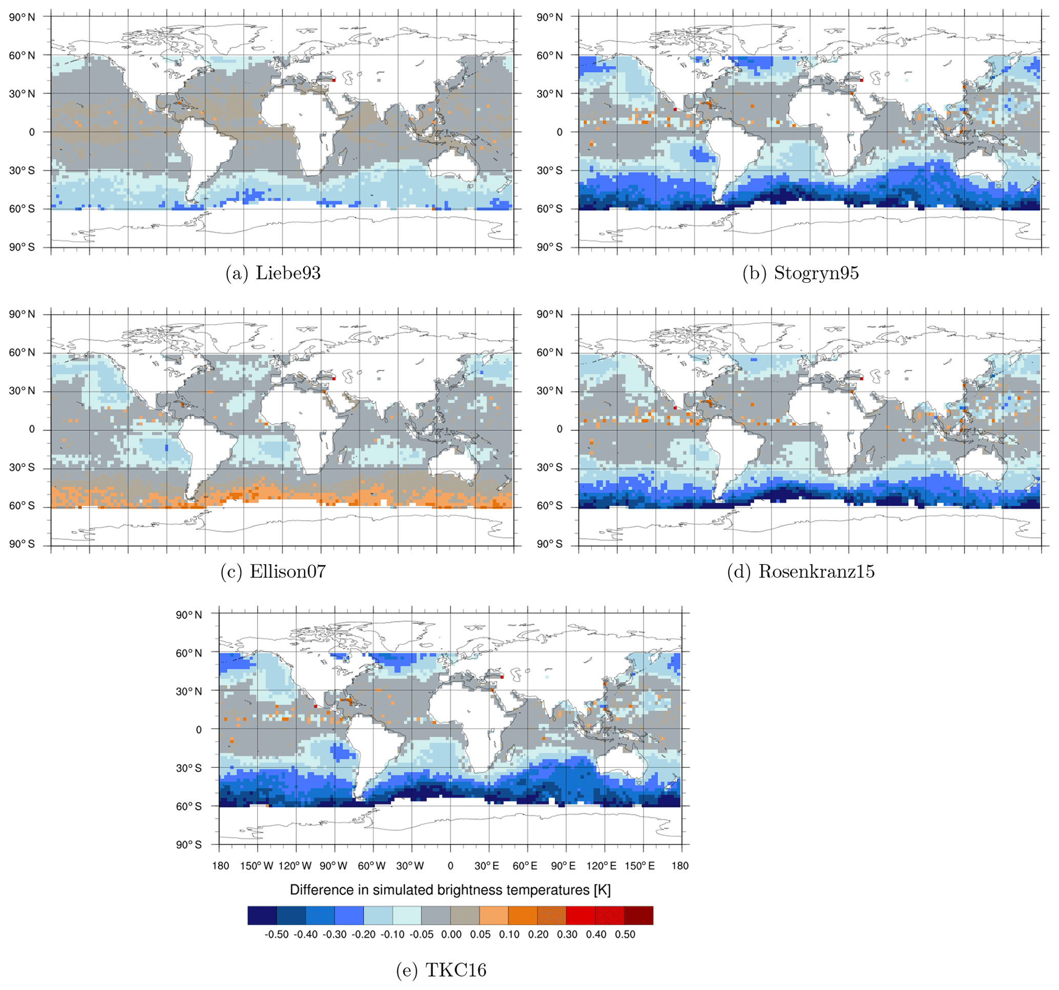
Figures 3, 4 and 5 show the geographical distribution of mean differences between the different permittivity models in simulated brightness temperature compared to Liebe89 at 37 v, 92 v and 150 h. The largest differences occur predominately in the midlatitudes and to a minor extent around the intertropical convergence zone (ITCZ), which is linked to the higher occurrence of supercooled liquid water in these regions. In the ITCZ, deep convective clouds prevail, which contain some supercooled liquid water. However, supercooled liquid water is clearly more frequent and influential on the simulated brightness temperatures at higher latitudes. Here, supercooled liquid water is found in fronts and in cold-air outbreak areas, which are areas with the largest changes (as shown in Sect. 3.3). In the higher latitudes, Stogryn95, Rosenkranz15 and TKC16 show a reduction in simulated brightness temperature at frequencies up to 150 GHz compared to Liebe89. Only Liebe93 shows an increase at 150 h despite a decrease at lower frequencies, and Ellison07 shows an increase at 92 v and 150 h despite a decrease at 37 v. This increase in brightness temperatures at high frequencies is due to higher absorption for temperatures below 260 K in the case of Liebe93 and due to higher absorption for temperatures around 270 K in the case of Ellison07 compared to Liebe89 (see Fig. 1c and d).
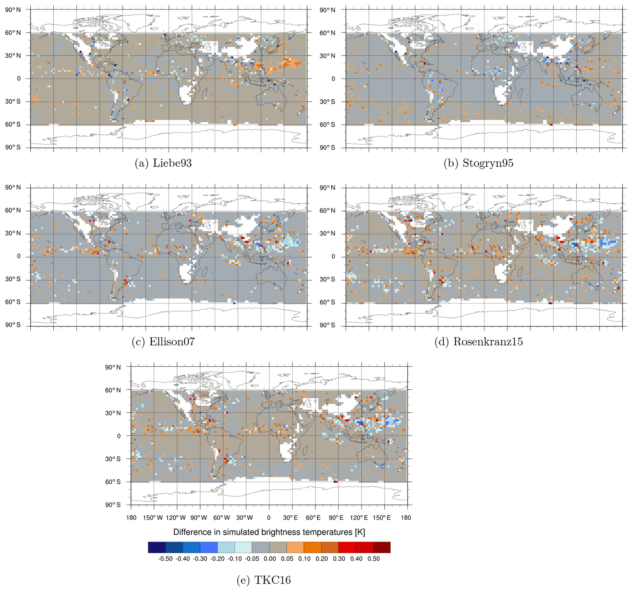
The sensitivity of absorption to the liquid water permittivity formulations is largest for high frequencies, as would be expected from Fig. 2. However, simulated brightness temperatures change only little for most regions at these frequencies, as can be seen for 183 ± 6 GHz, H polarised (183 ± 6 h) in Fig. 6. The reason for this behaviour is based in the weighting function at 183 ± 6 h peaking around 700 hPa, which makes it less sensitive to lower-lying supercooled liquid water clouds and more susceptible to the occurrence of snow or higher-level clouds, which are predominately composed of ice. In other words, the radiative transfer effects at 183 GHz are dominated by scattering from frozen hydrometeors. At 183 ± 6 h the only large differences in simulated brightness temperature are found in a few areas along the ITCZ or the western Pacific Ocean, associated with a higher occurrence of deep tropical convection, which must contain some supercooled liquid water.
In general, larger mean differences between the permittivity models can be seen for frequencies up to 150 GHz. The larger differences in absorption at frequencies up to 150 h GHz go in hand with the shift to higher temperatures in the spread among the different permittivity models if the frequency increases (as mentioned in Sect. 3.1). That means at 92 v changes in the absorption (and, hence, brightness temperature) can be seen for warmer clouds in the subtropics. For a discussion of the change in the difference between observed and simulated brightness temperatures (FG departures) see Appendix A.
3.3 Cold-air outbreaks
Despite small monthly mean differences in the simulated brightness temperature (or first guess, FG) among the six liquid water permittivity models, much larger differences in simulated brightness temperature can be seen if we focus specifically on supercooled liquid water clouds. An example is the high latitudes of the Southern Hemisphere during austral winter, which are marked by the occurrence of supercooled liquid water as illustrated for a 12 h assimilation window centred around 03:00 UTC on 30 August 2016 in Fig. 7. Here, the differences in FG between TKC16 and Liebe89 are shown at 92 v and at 183 ± 6 h, with the corresponding model cloud liquid water path, model snow water path and observation errors.
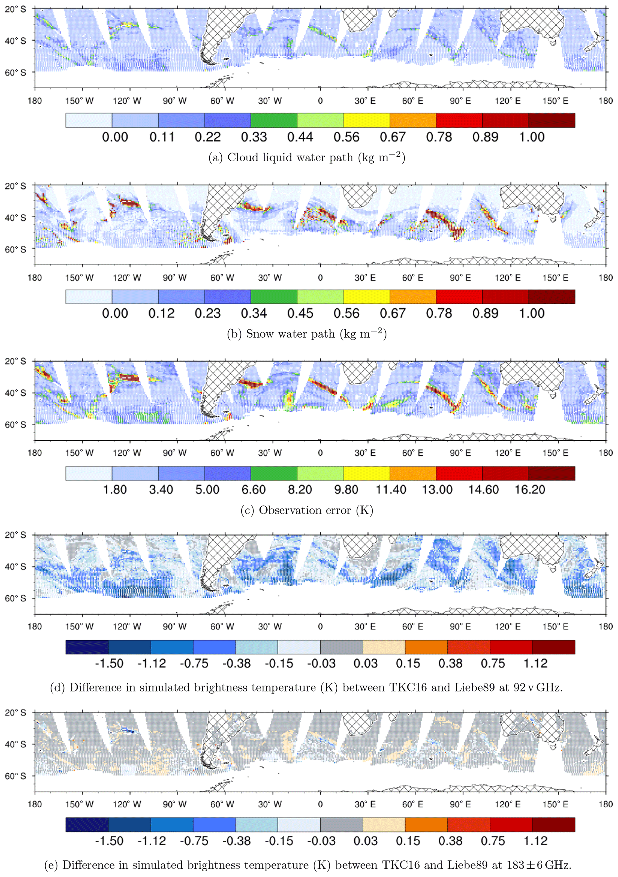
Figure 7Maps for (a) cloud liquid water path from the corresponding FG field, (b) snow water path from the corresponding FG field, (c) observation error with Liebe89, (d) difference in FG at 92 v between TKC16 and Liebe89 and (e) difference in FG at 183 ± 6 GHz between TKC16 and Liebe89 for areas of the southern midlatitudes to high latitudes excluding land and sea ice for a 12 h window centred at 03:00 UTC on 30 August 2016, co-located to SSMIS-F17 observations. Cross-hatched areas represent land and white areas have no data, e.g. due to screening or quality control (see Sect. 2.2)
The FG at 92 v simulated at SSMIS-F17 locations for TKC16 is reduced compared to Liebe89 by 0.5 to 1.5 K (Fig. 4d). Cadeddu and Turner (2011) show in their Fig. 2 that changes in brightness temperatures of this order happen for temperatures higher than −9 ∘C and for clouds with smaller liquid water amounts, of around 0.1 kg m−2. If temperatures were colder ( ∘C) or if the clouds were slightly thicker (around 0.25 kg m−2), the change in brightness temperature would already be 2 to 3 K. Their finding is consistent with the fact that the largest differences in simulated brightness temperatures at 92 v GHz occur in non-frontal cloud systems at higher latitudes characterised by liquid water of about 0.2 to 0.4 kg m−2. In contrast, the largest changes at 183 ± 6 h occur in specific conditions, e.g. at 30∘ S, 120∘ W. This could be related to cases of supercooled liquid water inside frontal systems.
The observed change in FG at 92 v of about 1 K is much smaller than the typical observation error of about 4 to 10 K in these regions (see Fig. 7c). Thus, using a different permittivity formulation than Liebe89 might only have a small impact on the analysis in a NWP system. The differences in simulated brightness temperatures seem small in comparison to the large differences among the permittivity models seen for supercooled liquid water clouds. However, in this case study, clouds with supercooled liquid water between 40 and 60∘ S are usually located at around 1 to 2 km in height inside the forecast model, where temperatures reach between approximately 260 to 270 K. That means observed changes in absorption are consistent with Fig. 2b, which shows small differences between models. However, it could be seen that clouds are located in much cooler locations south of 60∘ S, where microwave imager observations are currently not assimilated. Including these observations in the future, one might expect to see larger differences in simulated brightness temperature through the use of a new permittivity model.
As shown before, most permittivity models slightly reduce the simulated brightness temperature compared to Liebe89 with two exceptions, Ellison07 and Liebe93, which both increase the simulated brightness temperature at higher frequencies in the higher latitudes of the Southern Hemisphere. In order to find the best choice for the RTTOV-SCATT permittivity model used inside the IFS, we look at different measures to quantify the fit between model and observations and see whether it has improved. Here, results are based on the monitoring experiments.
4.1 Different measures of fit
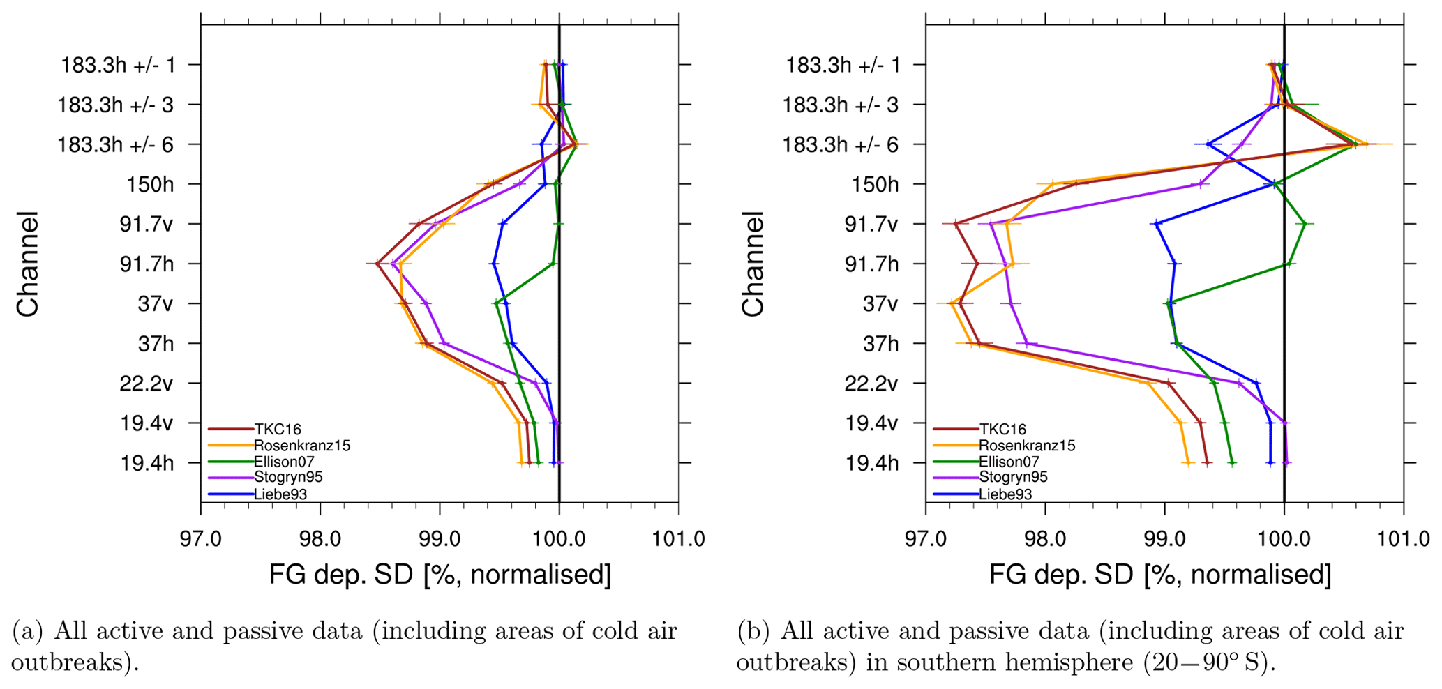
Figure 8Standard deviation in FG departure from SSMIS-F17 for different channels normalised by the standard deviation of results from Liebe89. The horizontal bars indicate a 95 % confidence range. Results cover the time period from 1 to 31 August 2016. Different colours refer to different permittivity models, as shown in the figure.
One measure of fit is the comparison of the standard deviation of FG departure using Liebe89 as a reference for observations from SSMIS-F17, as shown in Fig. 8. For most permittivity models the standard deviation in FG departure is reduced compared to Liebe89, as shown in Fig. 8a. The largest reduction occurs at 92 h for TKC16 of about 1.5 %. This signal is more pronounced in the Southern Hemisphere (Fig. 8b), where TKC16 shows a reduction of about 2.6 % at 92 h due to the stronger presence of supercooled liquid water clouds during austral winter. In the Southern Hemisphere, Ellison07 shows a significant increase in FG departure standard deviation at 92 v GHz and at 183 ± 6 h, whereas Rosenkranz15 and TKC16 show an increase at 183 ± 6 h, only. To study the effect introduced by different permittivity models in more detail, focus is put on the results from the Southern Hemisphere (20–90∘ S) for the remainder of this study. As discussed in Sect. 3.3, there is a higher occurrence of supercooled liquid water clouds during austral winter in the Southern Hemisphere and, hence, the effects through a change in permittivity model are more pronounced. Results would be similar for other regions with supercooled liquid water.
Typically, a reduction in the standard deviation in FG departure can be interpreted as a better fit between observations and first guess. However, for all-sky observations this measure is affected by the “double penalty” effect. That means better scores could be achieved if no clouds or precipitation are forecasted than if they are forecasted at the wrong location or wrong time (Geer and Baordo, 2014). Additionally, compensating biases could yield a reduction in standard deviation in FG departure even if the physical realism of the absorption model is getting worse; e.g. too much scattering could be compensated by too much absorption. An alternative measure which is resistant to the double-penalty effect (but unfortunately not to competing biases) is to evaluate fits between the model and observations looking at histograms of FG departure, as done in Fig. 9.
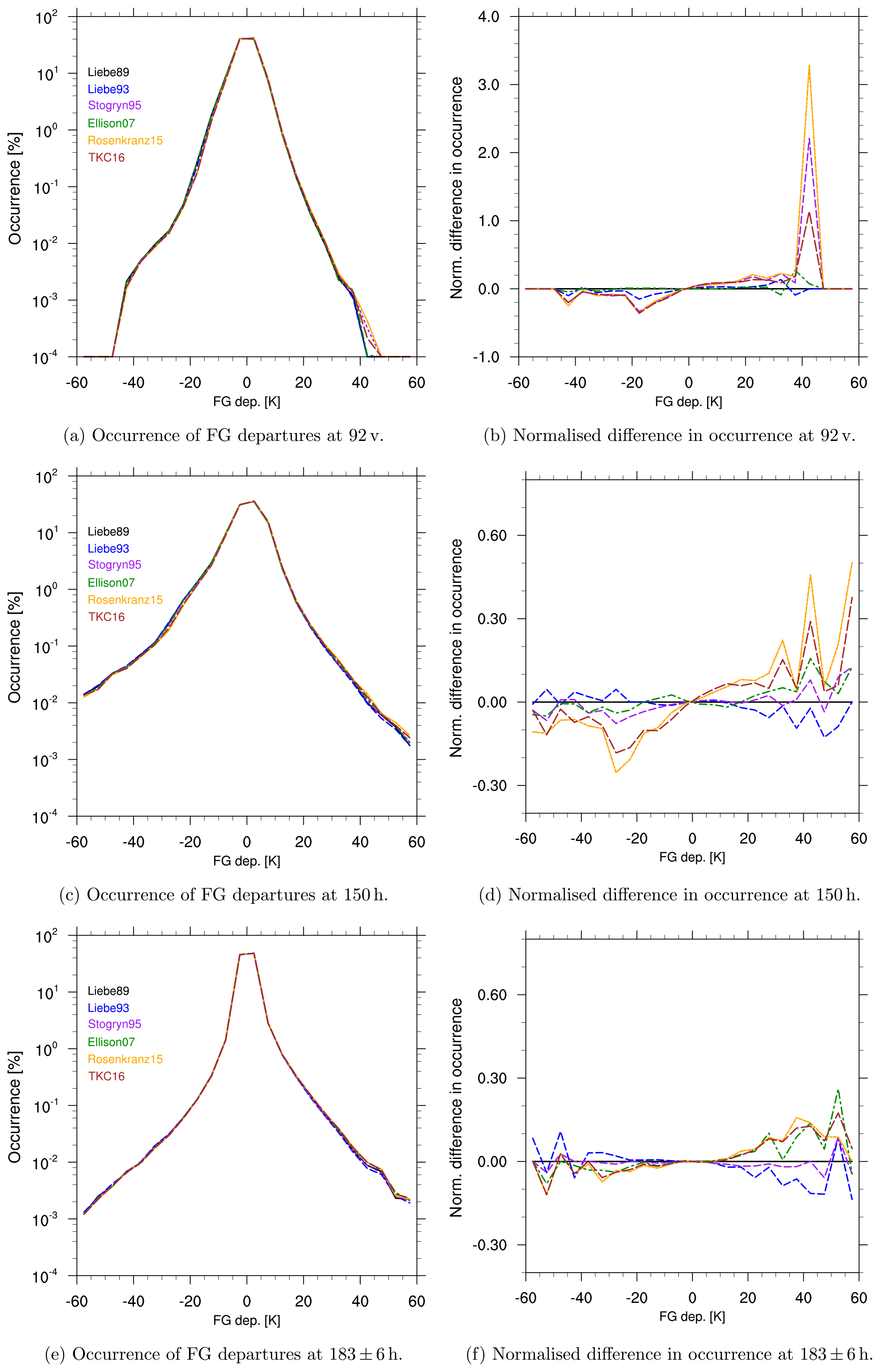
Figure 9Histograms of FG departure [K] using different liquid water permittivity models with the right panel showing the normalised difference for the newer permittivity models relative to Liebe89. Bin size is 5 K. Results cover the time period from 1 to 31 August 2016 for the Southern Hemisphere (20 to 90∘ S). Different colours refer to different permittivity models, as shown in the figure.
It can be seen that Liebe93, Stogryn95, Rosenkranz15 and TKC16 slightly reduce the number of occurrences of large negative FG departures and increase the number of occurrences of large positive departures compared to Liebe89 at 92 v (Fig. 9a and b), at 150 h (Fig. 9c and d) and at 37 v (not shown). At these channels Rosenkranz15 and TKC16 show the largest changes in numbers. This is not surprising as Rosenkranz15 and TKC16 reduce the simulated brightness temperature the most compared to the other permittivity models (see Table 3). At 183 ± 6 h only a small increase in the numbers at large positive FG departures can be seen for Ellison07, Rosenkranz15 and TKC16 (Fig. 9e and f) compared to Liebe89, which probably explains the degraded fits in FG departure standard deviation (Fig. 8). This increase can be explained by low absorption values of TKC16, Rosenkranz15 and Ellison07 compared to Liebe89 at low temperatures (supercooled liquid water), as shown in Fig. 2a. The low absorption causes smaller simulated brightness temperatures leading to an even larger difference between FG and the observations (more positive FG departures). From Figs. 6 and 7e it seems that these reduced brightness temperatures occur mostly in frontal systems in the Southern Hemisphere, where large FG departures are found more regularly, e.g. due to displacement errors between observations and the simulation.
To characterise large FG departures, the skewness can be used as done by Geer and Baordo (2014). If the skewness is positive the histogram of FG departures has a large tail to the right (more large negative FG departures than large positive FG departures). The larger the skewness the more large positive FG departures exist. Rosenkranz15 and TKC16 show the largest values in skewness in FG departure (see Fig. 10) at 37 v, larger than Liebe89. However, their standard deviation (and mean, not shown) in FG departure is significantly smaller, as shown before in Fig. 8b. At 92 v and 150 h the skewness is smaller than Liebe89, which is consistent with a reduced standard deviation. Only at 183 ± 6 h skewness and standard deviation are increased compared to Liebe89. In other words, the change in skewness is associated with the change in FG departure standard deviation for frequencies higher than 37 GHz.
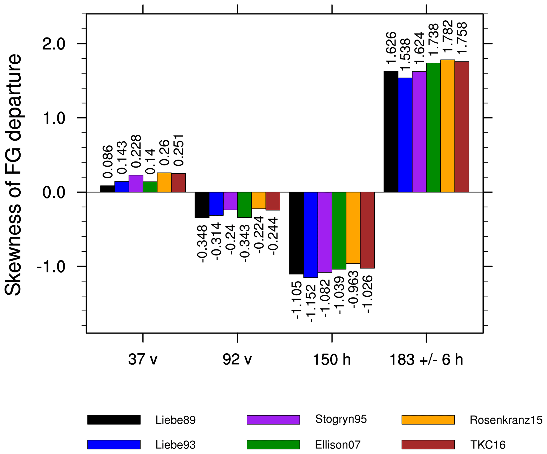
Figure 10Skewness in FG departure distribution for the different liquid water permittivity models at 37 v, 92 v, 150 h and 183 ± 6 h co-located to SSMIS-F17 observations over the time period 1 to 31 August 2016 for the Southern Hemisphere (SH: 20 to 90∘ S).
Nevertheless, the use of different permittivity models does not fundamentally change the shape of histograms of FG departure. If the spread among the permittivity models is interpreted as an indication of their likely uncertainty levels, permittivity errors are a minor factor and do not explain the bigger picture of the differences between observations and forecast model. The degradation in FG departure standard deviation at 183 ± 6 h is, however, genuine and is investigated in the next section.
4.2 Degradation at 183 ± 6 h
The degradation at 183 ± 6 h can be seen in a larger standard deviation in FG departure for TKC16, Rosenkranz15 and Ellison07 compared to Liebe89. The reduction in absorption and, hence, simulated brightness temperature causes larger differences compared to the observations, which has mostly been associated with cases of midlatitude frontal systems (not shown). Here, the compensating effect of absorption by liquid cloud droplets and scattering by ice and snow may play a key role. Figure 11a shows the normalised standard deviation of FG departure from SSMIS-F17 for samples with only liquid hydrometeors and a large cloud amount. Hereby, we use a symmetric measure of cloud amount C37 as defined in Geer and Bauer (2010), which is based on the polarisation difference at 37 GHz and is an average of the models and the observed cloud amount. Note that only the most intense convection shows 1 for C37. That means the chosen value of C37 > 0.05 should capture scenes with enough clouds, which allows us to avoid studying the effects of the non-cloudy condition.
Here, the degradation at 183 ± 6 h for Ellison07, Rosenkranz15 and TKC16 reduces to the same level as for the other permittivity models, with most of the other improvements remaining. Even though the sample size is reduced in Fig. 11a, results prove that scattering by frozen hydrometeors is related to the degradation at 183 ± 6 h. Figure 11b shows how the FG departure standard deviation at 183 ± 6 h changes with the ratio of frozen hydrometeor amount to total hydrometeor amount for the same sample. The higher this ratio, the more Ellison07, Rosenkranz15 and TKC16 become degraded, and Liebe93 and Stogryn95 become less degraded or are improved compared to Liebe89. If we plot the change in FG departure standard deviation at 183 ± 6 h as a function of integrated cloud liquid water (CWP) for only liquid clouds, we see that for Rosenkranz15, TKC16 and Liebe93 the FG departure standard deviation is comparable to that in Liebe89 or improves with an increase in CWP. For Ellison07 and Stogryn95 the fit degrades as CWP increases (not shown). This shows that the degradation only occurs in areas with frozen hydrometeors and strong scattering.

Figure 11Standard deviation in FG departure from SSMIS-F17 normalised by Liebe89 for (a) different channels for samples with no frozen hydrometeors containing some cloud (about 16.8 % of the full sample size from the Southern Hemisphere) and for (b) different ratios of the frozen hydrometeor amount versus total hydrometeor amount at 183 ± 6 h. The horizontal bars indicate a 95 % confidence range. Results cover all active and passive data (including areas of cold-air outbreaks) in the Southern Hemisphere (20–90∘ S) from 1 to 31 August 2016. Different colours refer to different permittivity models, as shown in the figure.
In general, absorption increases the brightness temperature at 183 ± 6 GHz, whereas scattering decreases for situations in which the (radiometrically cold) surface is partly visible. In these cases, any biases in the representation of absorption have the potential to be compensated by biases in the representation of scattering. If scattering is already excessive at 183 ± 6 h, then a reduction in absorption by using TKC16, Rosenkranz15 or Ellison07 would decrease the brightness temperature even more. In other words, the compensation effect of too much absorption and too much scattering would mean that TKC16, Rosenkranz15 and Ellison07 could erroneously appear worse compared to the other permittivity models, which show higher absorption values at 183 GHz. Here, two things could cause excessive scattering. Firstly, the frozen hydrometeor water content generated by the forecast model is too high and, secondly, the amount of scattering by the scattering model, e.g. in frontal systems, is too great. The latter case seems more likely when looking at the results by Geer and Baordo (2014). They show in their Fig. 8b that the sector snowflake shape used for snow in the scattering model inside RTTOV-SCATT produces positive FG departures around 1 K at 183 ± 6 GHz in midlatitudes to high latitudes. That suggests the scattering model causes brightness temperatures that are too low due to excessive scattering. This excessive scattering should explain the degradations seen for Ellison07, Rosenkranz15 and TKC16 at 183 ± 6 h in frontal systems at higher latitudes.
To properly assess the impact of the different liquid water permittivity models on the assimilation system, targeted assimilation experiments are performed, as described in Sect. 2.3. Two sets of experiments are conducted. The first set of assimilation experiments (plusSLW) uses the same configuration as the monitoring experiments, which uses supplementary observations containing cold-air outbreak areas and low water vapour areas, and allows the generation of additional supercooled liquid water clouds inside the forecast model. The second set of experiments (screen) simply uses the default set-up, which does not use observations containing cold-air outbreak areas and low water vapour areas but generates additional supercooled liquid water clouds inside the forecast model. In order to assess the impact the forecast scores and fits to the observations have been analysed. Results are only shown for Stogryn95 and Rosenkranz15, because Liebe93 and Ellison07 have been identified to show the smallest improvements (see Sect. 4), and TKC16 is very similar to Rosenkranz15.

Figure 12Standard deviation in FG departure in the Southern Hemisphere of ATMS, MHS and SSMIS for Rosenkranz15 and Stogryn95 normalised by Liebe89 for plusSLW and for screen. Different colours refer to different liquid water permittivity models, as shown in the figure. The horizontal bars indicate 95 % confidence range. Results cover the time period from 1 June to 30 September 2016.
It is found that using different formulations of permittivity shows a neutral impact on forecast scores in terms of a change in root-mean-square error in humidity, temperature and wind in the long- and short-term for plusSLW and screen (not shown). This is likely related to the fact that the introduced change in simulated brightness temperatures is small, both relative to the observation error (e.g. Fig. 7c) and relative to differences between observations and forecast model (Fig. 9). However, fits of the first-guess forecast (T+12 h forecast) to humidity sensitive observations are altered through a change in the liquid water permittivity model. For example, Rosenkranz15 and Stogryn95 improve fits to the humidity sensitive channels of the Advanced Technology Microwave Sounder (ATMS; channels 18–22) in the Southern Hemisphere for plusSLW compared to Liebe89 (Fig. 12a). An improvement seen for ATMS is the result of an improved first-guess humidity field because ATMS is only assimilated in clear-sky conditions (Sect. 2.2) and, hence, cannot be affected directly by a change in liquid water permittivity model inside the RTTOV-SCATT. It is notable that improvements have not been detected in the humidity field in the analysis-based verification mentioned earlier. However, analysis-based verification can be unreliable at short ranges due to correlations between the forecast and the reference, so we would place more reliance on verification against observations here.
In contrast to ATMS, the Microwave Humidity Sounding (MHS) instrument is assimilated under all-sky conditions. Here, using Rosenkranz15 degrades the fit to channel 5 (183 ± 7 GHz, V polarised), whereas Stogryn95 improves it to a similar extent in plusSLW and in screen (Fig. 12b and d, respectively). The degradation for Rosenkranz15 is most likely caused by the excess scattering in midlatitude frontal systems, which is not compensated as much by an excess in absorption as in Liebe89 (discussed in Sect. 4). A similar change is found for most 183 GHz channels of the Sondeur Atmospherique du Profil d'Humidite Intertropicale par Radiometrie (SAPHIR) for both permittivity models in plusSLW (not shown).
As expected, improved fits to microwave imagers are found, e.g. in fits to SSMIS (Fig. 12c), similarly to the GPM Microwave Imager (GMI) and the Advanced Microwave Scanning Radiometer 2 (AMSR2, not shown). Here, Rosenkranz15 shows larger improvements than Stogryn95, even for screen. Interestingly, only when cold-air outbreak areas and low water vapour areas are included (plusSLW) is a degradation found at 183 ± 6 h (channel 9 SSMIS) for Rosenkranz15. A likely explanation could be that the screening also removes some of those midlatitude frontal areas with the moderate brightness temperature changes (as seen in Fig. 7e), not just cold-air outbreaks. The reason is that 80 % of cold-air outbreaks occur in association with a cyclonic flow (Papritz et al., 2015).
Additionally, mean changes in the bias in FG departure at 37 and at 92 v have been analysed for microwave imagers in the Southern Hemisphere (not shown). For SSMIS the bias changed by about 0.2 K, which led to a reduction in the bias in plusSLW to 0 K and a slight increase to 0.3 K for screen. For GMI and AMSR2 the bias between −0.25 and −0.5 K has been reduced by about 0.2 K for both screen and plusSLW. Fits to temperature-sensitive observations (e.g. the Advanced Microwave Sounding Unit – A, AMSU-A) and wind (e.g. atmospheric motion vectors) are neutrally affected by the different choices of permittivity models for screen and plusSLW (not shown).
We have studied the effect of six different permittivity formulations on simulated brightness temperatures (first guess, FG) and the impact on the assimilation system using the Integrated Forecast System (IFS). As shown already, e.g. by Kneifel et al. (2014), newer liquid water permittivity models are known to give significant lower values of absorption for supercooled liquid water at microwave frequencies above 19 GHz.
A model configuration is used which allows the generation of more and colder supercooled liquid water than available in earlier IFS versions. Firstly, the limit of the existence of supercooled liquid water has been changed from −23 to −38 ∘C for convective mixed-phase clouds and, secondly, the model physics upgrade in IFS cycle 45R1 allows the generation of purely supercooled liquid water inside surface-driven shallow clouds. This change was motivated by findings showing a lack of supercooled liquid water in cold-air outbreak regions inside the forecast model (Forbes et al., 2016). Even though this configuration misses the generation of some supercooled liquid water in congestus clouds and deep convection clouds, it seems good enough to study the impact of different liquid water permittivity models including clouds with supercooled liquid water. Additionally, microwave imager observations in these regions have been included in the assimilation, which are usually screened due to a systematic model bias.
Most of the permittivity formulations reduce the simulated brightness temperatures slightly compared to Liebe89 due to their smaller values in absorption. The largest reduction in simulated brightness temperatures is observed in areas with supercooled liquid water, such as cold-air outbreaks. There are just two exceptions: Liebe93 and Ellison07. Due to slightly larger values in absorption for higher microwave frequencies, Liebe93 and Ellison07 increase the simulated brightness temperature in areas of supercooled liquid water. The newer permittivity formulations by Rosenkranz15 and TKC16 show the largest reductions together with Stogryn95. Using TKC16 reduces the simulated brightness temperature by about 0.5 to 1.5 K at 92 v for regions with supercooled liquid water. A forecast model allowing the generation of purely supercooled liquid water congestus clouds or deep convection might be able to reduce the brightness temperatures even further. However, this cannot be concluded from the set of experiments presented in this study, and more targeted studies are necessary to confirm this hypothesis.
On a global scale, the differences between the permittivity models are small and cannot explain the main discrepancy between the model and observations. However, the biggest improvements in terms of observational fits to microwave imagers could be seen for the new permittivity models TKC16 and Rosenkranz15 for frequencies below 183 GHz. Some degradation at 183 ± 6 GHz from SSMIS and MHS has been seen for Ellison07, Rosenkranz15 and TKC16. This degradation seems to occur in clouds containing some supercooled liquid water in midlatitude frontal systems. Here, the compensating biases in the scattering model and in the absorption model most likely play a major part. Geer and Baordo (2014) have shown that the current choice of sector snowflake shape and the choice in particle size distribution in the scattering model inside RTTOV-SCATT introduces excessive scattering in the higher latitudes. This excessive scattering seems to be less compensated through liquid water absorption when using Ellison07, Rosenkranz15 or TKC16. To address this apparent degradation, studies are planned to re-examine how the forecast model represents clouds and precipitation, how the data assimilation framework handles cloud- and precipitation-affected observations, how we can improve the construction of the observation operator and how observation errors are treated in the all-sky assimilation at ECMWF (Geer et al., 2017).
To properly test the impact of the different permittivity models on the assimilation system, targeted assimilation experiments have been conducted. It could be shown that the forecast is only neutrally affected by a change in permittivity model, which is probably due to the large observation errors relative to changes in brightness temperatures caused by different liquid water permittivity models. Nevertheless, improved fits to independent observations, like the humidity channels of ATMS, are found for the Southern Hemisphere. In the future, when forecast models are capable of generating enough supercooled liquid water clouds and the assimilation system uses microwave observations in these regions, the impact of the permittivity formulation will be even more crucial. But most of the observational fits to humidity and cloud sensitive observations are already improved and forecast scores are not degraded by using the liquid water permittivity formulation by Stogryn et al. (1995), Rosenkranz (2015) or Turner et al. (2016).
In light of those results – (i) a small impact on simulated brightness temperatures in regions with a relatively large systematic error, (ii) a neutral impact on forecast scores and (iii) difficulty in balancing good and bad changes because of the compensating biases in scattering and absorption – one has to ask whether this sort of NWP closure study is actually able to find the “best” liquid water permittivity model. We would argue that it is possible, at least, to reject the worst models. Such a closure study has the unique ability to quantify the global effect of supercooled liquid water permittivity changes in a high-quality model atmosphere and not just locally as done through comparisons with observations from ground or under idealised conditions in laboratory experiments. Additionally, it is found that using different liquid water permittivity models has an effect on independent data sets (e.g. for ATMS). Lastly, it is reassuring that the newest permittivity models, Rosenkranz15 and TKC16, which are based among other things on the most up-to-date observations, also have the best fits to the microwave imagers SSMIS, GMI and AMSR2, being slightly better than Stogryn95. Our results indicate that either Rosenkranz15 or TKC16 should be used inside RTTOV-SCATT, with both showing a similar level of improvement. For now that would encompass microwave frequencies, which are less prone to compensating biases in the scattering and absorption model, i.e. below 183 GHz. Looking into the future, where we want to assimilate microwave frequencies up to 1 THz, we favour the use of the Rosenkranz15 permittivity model inside RTTOV-SCATT, as it has been constructed for higher microwave frequencies, whereas TKC16 is only valid up to 500 GHz.
The RTTOV observation operator is copyrighted by EUMETSAT but is available free of charge to registered users via https://www.nwpsaf.eu/site/software/rttov/ (last access: 16 January 2019). The ECMWF data assimilation system is copyrighted by ECMWF and access to these systems (and the data provided by them) is possible through agreement with its member state national hydrometeorological organisations.
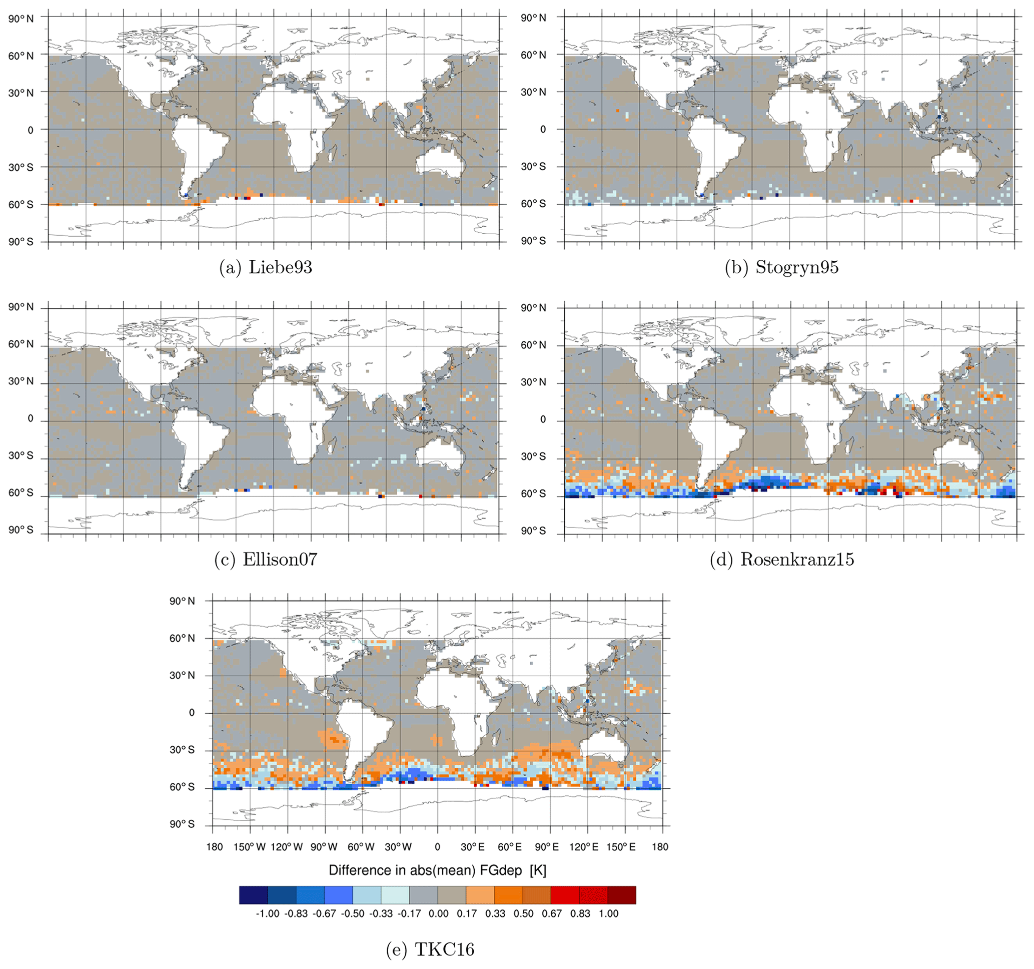
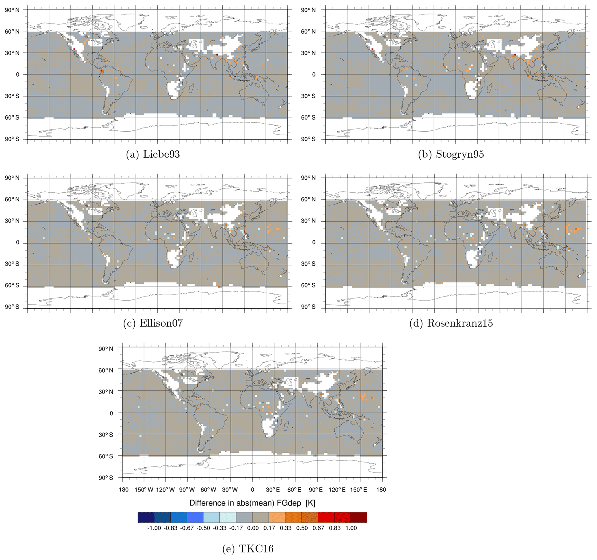
Figures A1, A2, A3 and A4 show the geographical distribution of mean differences between the different permittivity models in absolute values of observed minus simulated brightness temperatures (FG departures) compared to Liebe89 at 37 v, 92 v, 150 h and 183 ± 6 h respectively. Here, absolute values are calculated using the resulting binned means. The largest changes in FG departure can be seen for Stogryn95, Rosenkranz15 and TKC16 in the southern midlatitudes to high latitudes for frequencies up to 150 GHz. Hereby, the absolute value in FG departure is reduced by about 0.3 and 0.6 K at 37 v and at 92 v, respectively, with an additional increase in FG departure of about 0.3 K in the northern midlatitudes to high latitudes at 92 v. At 150 h a slight increase in FG departure is shown for the southern midlatitudes and a decrease is shown for the southern higher latitudes of about 0.6 K for Rosenkranz15 and TKC16, only. No large changes can be seen for 183 ± 6 h. The mean changes in FG departure are plotted for the monitoring experiments which include SSMIS-F17 observations from areas, which are usually screened in the default set-up as described in Sect. 2.3.3. That means that in these plots only changes in FG departure due to a change in the observation operator are highlighted.
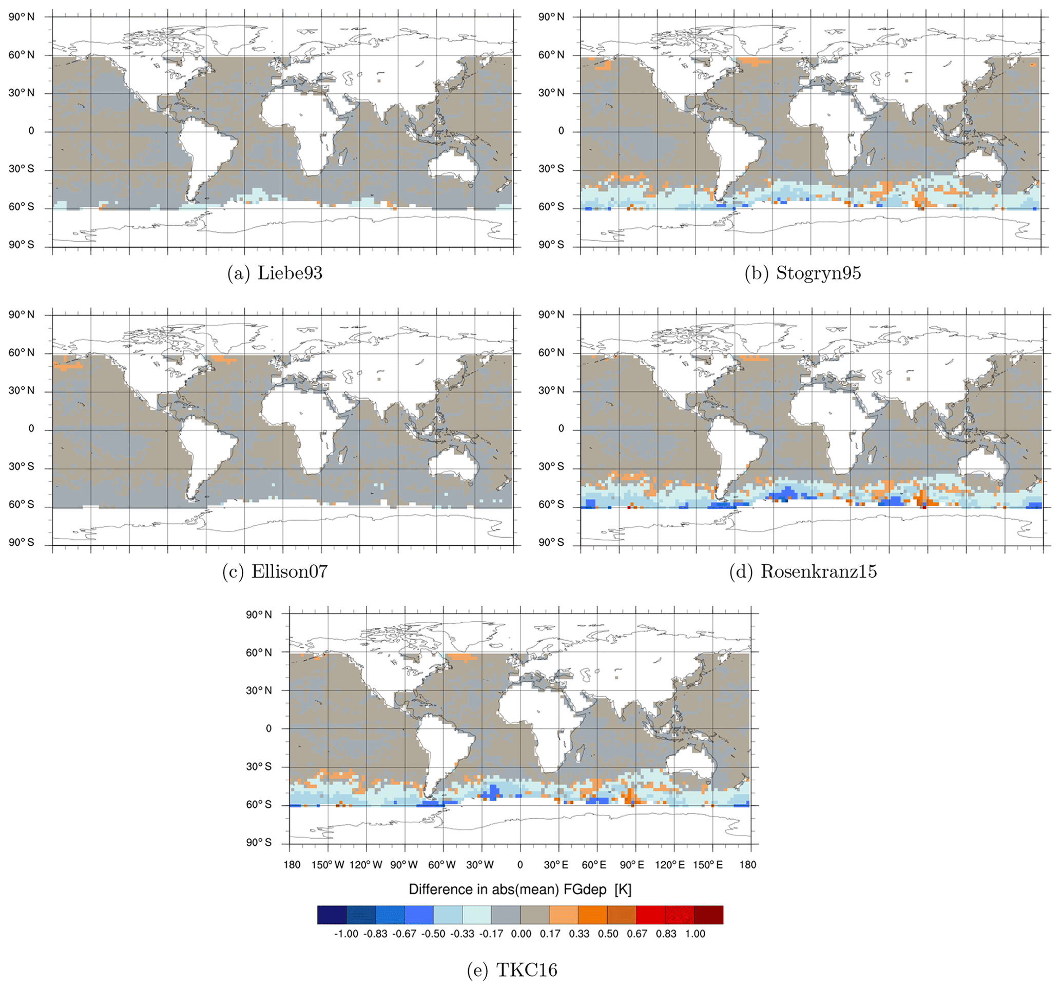
Figure A1Maps of differences in absolute values of observed minus simulated brightness temperatures [K] between the newer liquid water permittivity models and the current Liebe89 for 37 v brightness temperatures co-located to corresponding SSMIS-F17 observations. Means are computed in each 2.5∘lat × 2.5∘long bin and over the time period 1 to 31 August 2016. White areas correspond to areas in which data are not assimilated, as mentioned in Sect. 2.2.
KL contributed to the conceptualisation, investigation, methodology, software, visualisation and writing. AG contributed to the conceptualisation, methodology, writing and software.
The authors declare that they have no conflict of interest.
The work of Katrin Lonitz at ECMWF is funded by the EUMETSAT fellowship
programme. Stefan Kneifel is thanked for making his code available for the Liebe93,
Stogryn95 and Ellison07 permittivity models. Robin Hogan is
acknowledged for encouraging the authors to undertake this study. The authors
also thank two anonymous reviewers for their thorough reviews.
Edited by: Domenico Cimini
Reviewed by: two anonymous referees
Bauer, P.: Including a melting layer in microwave radiative transfer simulation for cloud, Atmos. Res., 57, 9–30, 2001. a
Bauer, P., Moreau, E., Chevallier, F., and O'Keeffe, U.: Multiple-scattering microwave radiative transfer for data assimilation applications, Q. J. Roy. Meteorol. Soc., 132, 1259–1281, 2006. a, b
Bauer, P., Geer, A. J., Lopez, P., and Salmond, D.: Direct 4D-Var assimilation of all-sky radiances, Part I: Implementation, Q. J. Roy. Meteorol. Soc., 136, 1868–1885, 2010. a, b
Bodas-Salcedo, A., Andrews, T., Karmalkar, A. V., and Ringer, M. A.: Cloud liquid water path and radiative feedbacks over the Southern Ocean, Geophys. Res. Lett., 43, 10938–10946, https://doi.org/10.1002/2016GL070770, 2016. a
Cadeddu, M. P. and Turner, D. D.: Evaluation of Water Permittivity Models From Ground-Based Observations of Cold Clouds at Frequencies Between 23 and 170 GHz, IEEE T. Geosci. Remote, 49, 2999–3008, 2011. a, b
Debye, P.: Polare Molekeln, S. Hirzel, Leipzig, 1929. a
ECMWF: PART IV: PHYSICAL PROCESSES, in: IFS Documentation CY43R3, ECMWF, 2017. a
Ellison, W.: Permittivity of Pure Water at Standard Atmospheric Pressure over the Frequency Range 0–25 THz and the Temperature Range 0–100 ∘C, J. Phys. Chem. Ref. Data, 36, 1–18, 2007. a, b, c, d, e, f, g
Forbes, R., Geer, A. J., Lonitz, K., and Ahlgrimm, M.: Reducing systematic errors in cold-air outbreaks, ECMWF newsletter, 146, 17–22, 2016. a, b, c
Geer, A. J. and Bauer, P.: Enhanced use of all-sky microwave observations sensitive to water vapour, cloud and precipitation, ECMWF Tech. Memo., 620, 2010. a
Geer, A. J. and Bauer, P.: Observation errors in all-sky data assimilation, Q. J. Roy. Meteorol. Soc., 137, 2024–2037, https://doi.org/10.1002/qj.830, 2011. a
Geer, A. J. and Baordo, F.: Improved scattering radiative transfer for frozen hydrometeors at microwave frequencies, Atmos. Meas. Tech., 7, 1839–1860, https://doi.org/10.5194/amt-7-1839-2014, 2014. a, b, c, d, e
Geer, A. J., Bauer, P., and O'Dell, C.: A Revised Cloud Overlap Scheme for Fast Microwave Radiative Transfer in Rain and Cloud, J. App. Meteor. Clim., 48, 2257–2270, 2009. a
Geer, A. J., Ahlgrimm, M., Bechtold, P., Bonavita, M., Bormann, N., English, S., Fielding, M., Forbes, R., Hogan, R., Hólm, E., Janiskova, M., Lonitz, K., Lopez, P., Matricardi, M., Sandu, I., and Weston, P.: Assimilating observations sensitive to cloud and precipitation, ECMWF, Tech. Memo 815, 2017. a
Geer, A. J., Lonitz, K., Weston, P., Kazumori, M., Okamoto, K., Zhu, Y., Liu, E. H., Collard, A., Bell, W., Migliorini, S., Chambon, P., Fourrié, N., Kim, M.-J., Köpken-Watts, C., and Schraff, C.: All-sky satellite data assimilation at operational weather forecasting centres, Q. J. Roy. Meteorol. Soc., 144, 1191–1217, https://doi.org/10.1002/qj.3202, 2018. a
Heymsfield, A. J., Miloshevich, L. M., Slingo, A., Sassen, K., and Starr, D. O.: An Observational and Theoretical Study of Highly Supercooled Altocumulus, J. Atmos. Sci., 48, 923–945, https://doi.org/10.1175/1520-0469(1991)048<0923:AOATSO>2.0.CO;2, 1991. a, b
Kazumori, M. and English, S.: Use of the ocean surface wind direction signal in microwave radiance assimilation, Q. J. Roy. Meteorol. Soc., 141, 1354–1375, https://doi.org/10.1002/qj.2445, 2015. a
Kneifel, S., Redl, S., Orlandi, E., Löhnert, U., Cadeddu, M. P., Turner, D. D., and Chen, M.-T.: Absorption Properties of Supercooled Liquid Water between 31 and 225 GHz: Evaluation of Absorption Models Using Ground-Based Observations, J. Appl. Meteor. Climatol., 53, 1028–1045, https://doi.org/10.1175/JAMC-D-13-0214.1, 2014. a, b, c, d, e, f
Kunkee, D. B., Poe, G. A., Boucher, D. J., Swadley, S. D., Hong, Y., Wessel, J. E., and Uliana, E. A.: Design and Evaluation of the First Special Sensor Microwave Imager/Sounder, IEEE T. Geosci. Remote, 46, 863–883, 2008. a
Liebe, H. J., Hufford, G. A., and Cotton, M. G.: Propagation modeling of moist air and suspended water/ice particles at frequencies below 1000 GHz, in: AGARD, Atmospheric Propagation Effects Through Natural and Man-Made Obscurants for Visible to MM-Wave Radiation, 11 pp., (SEE N94-30495 08-32), 1993. a, b, c, d, e
Liebe, H. J.: MPM – An atmospheric millimeter-wave propagation model, Int. J. Infrared. Milli., 10, 631–650, https://doi.org/10.1007/BF01009565, 1989. a, b, c, d, e, f, g
Lonitz, K. and Geer, A.: EUMETSAT/ECMWF Fellowship Programme Research Report: New screening of cold-air outbreak regions used in 4D-Var all-sky assimilation, Tech. Rep. 35, 2015. a, b
Papritz, L., Pfahl, S., Sodemann, H., and Wernli, H.: A Climatology of Cold Air Outbreaks and Their Impact on Air–Sea Heat Fluxes in the High-Latitude South Pacific, J. Climate, 28, 342–364, https://doi.org/10.1175/JCLI-D-14-00482.1, 2015. a
Rosenkranz, P. W.: A Model for the Complex Dielectric Constant of Supercooled Liquid Water at Microwave Frequencies, IEEE T. Geosci. Remote, 53, 1387–1393, https://doi.org/10.1109/TGRS.2014.2339015, 2015. a, b, c, d, e, f, g, h, i, j
Saunders, R., Matricardi, M., and Brunel, P.: An improved fast radiative transfer model for assimilation of satellite radiance observations, Q. J. Roy. Meteorol. Soc., 125, 1407–1425, 1999. a
Stogryn, A., Bull, H., Rubayi, K., and Iravanchy, S.: The microwave permittivity of sea and fresh water, Aerojet Internal Report, GenCorp Aerojet, Azusa, CA, 24 pp., 1995. a, b, c, d, e, f, g, h
Turner, D. D., Kneifel, S., and Cadeddu, M. P.: An Improved Liquid Water Absorption Model at Microwave Frequencies for Supercooled Liquid Water Clouds, J. Atmos. Ocean. Tech., 33, 33–44, https://doi.org/10.1175/JTECH-D-15-0074.1, 2016. a, b, c, d, e, f, g, h, i