the Creative Commons Attribution 4.0 License.
the Creative Commons Attribution 4.0 License.
 | 22 Aug 2019
UK greenhouse gas measurements at two new tall towers for aiding emissions verification
Ann R. Stavert
Simon O'Doherty
Kieran Stanley
Dickon Young
Alistair J. Manning
Mark F. Lunt
Christopher Rennick
Tim Arnold
Under the UK-focused Greenhouse gAs and Uk and Global Emissions (GAUGE) project, two new tall tower greenhouse gas (GHG) observation sites were established in the 2013/2014 Northern Hemispheric winter. These sites, located at existing telecommunications towers, utilized a combination of cavity ring-down spectroscopy (CRDS) and gas chromatography (GC) to measure key GHGs (CO2, CH4, CO, N2O and SF6). Measurements were made at multiple intake heights on each tower. CO2 and CH4 dry mole fractions were calculated from either CRDS measurements of wet air, which were post-corrected with an instrument-specific empirical correction, or samples dried to between 0.05 % H2O and 0.3 % H2O using a Nafion® dryer, with a smaller correction applied for the residual H2O. The impact of these two drying strategies was examined. Drying with a Nafion® dryer was not found to have a significant effect on the observed CH4 mole fraction; however, Nafion® drying did cause a 0.02 µmol mol−1 CO2 bias. This bias was stable for sample CO2 mole fractions between 373 and 514 µmol mol−1 and for sample H2O up to 3.5 %. As the calibration and standard gases are treated in the same manner, the 0.02 µmol mol−1 CO2 bias is mostly calibrated out with the residual error (≪0.01 µmol mol−1 CO2) well below the World Meteorological Organization (WMO) reproducibility requirements. Of more concern was the error associated with the empirical instrument-specific water correction algorithms. These corrections are relatively stable and reproducible for samples with H2O between 0.2 % and 2.5 %, CO2 between 345 and 449 µmol mol−1, and CH4 between 1743 and 2145 nmol mol−1. However, the residual errors in these corrections increase to > 0.05 µmol mol−1 for CO2 and > 1 nmol mol−1 for CH4 (greater than the WMO internal reproducibility guidelines) at higher humidities and for samples with very low (< 0.5 %) water content. These errors also scale with the absolute magnitude of the CO2 and CH4 mole fractions. As such, water corrections calculated in this manner are not suitable for samples with low (< 0.5 %) or high (> 2.5 %) water contents and either alternative correction methods should be used or partial drying or humidification considered prior to sample analysis.
- Article
(3833 KB) - Full-text XML
-
Supplement
(4668 KB) - BibTeX
- EndNote


The adverse effects of anthropogenically driven increases in greenhouse gas concentrations on global temperatures and climate have been well established (IPCC, 2013). Governmental efforts to curb these emissions include the UK 2008 Climate Change Act, which will soon be amended to require the UK to produce net-zero emissions by 2050 (Parliament of the United Kingdom, 2008, Chapter 27). This in turn motivated the Greenhouse gAs Uk and Global Emissions (GAUGE) project, which aimed to better quantify the UK carbon dioxide (CO2), methane (CH4) and nitrous oxide (N2O) emissions. These new emission estimates would then be used to assess the impact of emission abatement and reduction strategies. Key to the GAUGE project was combining new and existing GHG data streams, including high-density regional observation studies, tall tower sites, moving platforms (ferry and aircraft) and satellite observations, with innovative modelling approaches.
This paper describes the establishment of two new UK GHG tall tower (TT) sites funded under the GAUGE project. Here we provide an analysis of the observations made at the sites and investigate the error associated with empirical instrument-specific water correction algorithms and the Nafion®-based sample drying approach used at these TT sites. A further paper, currently in preparation, will discuss the integration of these new sites with the existing UK Deriving Emissions linked to Climate Change (DECC) network (Stanley et al., 2018) funded by the UK Department of Business, Energy and Industrial Strategy (BEIS) and provide a full uncertainty analysis for data collected at all the DECC–GAUGE sites. A second companion paper, also in preparation, will discuss the integration and inter-calibration of all the CO2, CH4, CO, N2O and SF6 data streams including near surface, tall tower, ferry and aircraft measurements along with an analysis of the impact of identified site biases on UK GHG emission estimates.
Like the UK DECC network, the new sites, Bilsdale (BSD) and Heathfield (HFD), are equipped with a combination of cavity ring-down spectrometer (CRDS) and gas chromatograph (GC) instrumentation (Stanley et al., 2018). These instruments, along with the associated calibration gases (linked to WMO calibration scales) and automated sampling systems are located at the base of telecommunication towers within the UK. Further details of the sites and instruments used along with a description of the data collected to date are provided in the subsequent sections.
The precision, stability, relative autonomy and robustness of CRDS instrumentation has led to a rapid increase in it's deployment in global, continental and regional GHG monitoring networks including the GAUGE network, the European Integrated Carbon Observing System (ICOS) (Yver Kwok et al., 2015) and the Indianapolis Flux Experiment (INFLUX) (Turnbull et al., 2015). These instruments also claim the advantage of being able to measure undried (“wet”) air samples, which are then post-corrected to “dry” values using an inbuilt algorithm (Rella, 2010).
Initially, it was hoped that the inbuilt water correction would remove the need for sample drying, inherent in most other methods (e.g. FTIR or NDIR) but subsequent studies questioned its stability over time and between instruments (Yver Kwok et al., 2015; Chen et al., 2010; Winderlich et al., 2010). In response to this, researchers have typically developed their own water corrections or have returned to sample drying in order to minimize the effect (Welp et al., 2013; Winderlich et al., 2010; Schibig et al., 2015; Rella et al., 2013). As such the examination of any errors or biases induced by drying and water correction methods is essential for fully quantifying the uncertainty of CRDS measurements.
For ease of servicing, the CRDS instrumentation at GAUGE and UK DECC Network sites was initially deployed using an identical drying method to that of the co-located GC instrumentation. This method relied on drying the sample with a Nafion® water-permeable membrane in combination with dry zero air as a counter purge gas. Here, due to the moisture gradient between the sample and the counter purge, the water passed from the wet sample through the membrane to the dry counter purge. Drying in this manner has a history of successful application for the measurements of halocarbons (Foulger and Simmonds, 1979), N2O (Prinn et al., 1990) and SF6 (Fraser et al., 2004). However, studies have found that CO2 and CH4 can also pass across a dry Nafion® membrane (Chiou and Paul, 1988) and that this transport increases with the water saturation of the membrane (Naudy et al., 2014). As the transport process is driven by a partial pressure difference between the sample and counter purge gas, it is possible that changes in the sample CO2 and CH4 mole fraction relative to the counter purge gas, along with the water (H2O) content of the sample, may alter the magnitude of any cross-membrane leakage.
A study by Welp et al. (2013) examined this issue and concluded that the leakage was small and well within the WMO compatibility guidelines. However, the drying approach used by Welp et al. (2013) is not directly comparable to that of the GAUGE sites as they used dry sample gas as the counter purge rather than zero air. That study also only examined two water contents (0 % or 2 % H2O) and conducted only dry (0 % H2O) experiments on samples with CO2 and CH4 mole fractions above ambient concentrations. Considering the importance of water in gas transport across the membrane (Chiou and Paul, 1988) and the range of water contents observed in undried air samples measured within the DECC–GAUGE network (up to 3.5 % H2O), further investigation of this issue was required.
As such, this paper also aims to quantify the magnitude of Nafion® CO2 and CH4 transport using the drying method used at the DECC–GAUGE TT sites along with errors associated with instrument-specific water corrections. It also examines how these might change within the range of H2O, CO2 and CH4 mole fractions typically observed at these sites. The importance of these errors is assessed in comparison to the WMO internal reproducibility guidelines (WMO, 2018), which incorporate not only the instrumental precision but also uncertainties related to other components such as sample collection and measurement including drying. These internal reproducibility guidelines are typically half the WMO recommended compatibility goals, which, unlike the reproducibility guidelines, are driven by the need for compatibility between data sets.
2.1 Site descriptions
Two new tall tower sites, Heathfield (HFD; 50.977∘ N, 0.231∘ E) and Bilsdale (BSD; 54.359∘ N, 1.150∘ W), were established at existing telecommunication towers in December 2013 and January 2014 respectively. The general set-up of these sites is similar to that described for the DECC sites in Stanley et al. (2018) and the locations of these two new sites relative to the sites described in Stanley et al. (2018) are shown in Fig. 1.
The Heathfield tower is located in rural East Sussex, 20 km from the coast and 157.3 m above sea level. The closest large conurbation (Royal Tunbridge Wells) is located 17 km NNE from the tower. The area surrounding the tower is > 90 % woodland and agricultural area with some residential (0.7 %) and light industrial areas (0.3 %) (East Sussex in figures, 2006). Notable local industry includes a large horticultural nursery located only 200 m north of the tower.
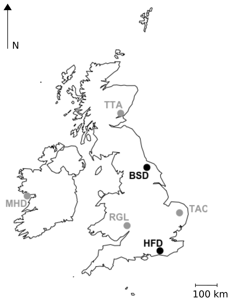
Figure 1Locations of the GAUGE Bilsdale (BSD) and Heathfield (HFD) sites, shown in black, and the UK DECC Mace Head (MHD), Ridge Hill (RGL), Tacolneston (TAC) and Angus (TTA) sites, shown in grey.
Bilsdale is a remote moorland plateau site within the North York Moors National Park. The base of the tower is located 379.1 m a.s.l. It is 25 km NNW of Middlesbrough (the closest large urban area) and 30 km from the coast. The tower is situated in a predominantly rural area, including moorland, woodland, forest and farmland (North York Moors National Park Authority, 2012; Chris Blandford Associates, 2011).
Inverted stainless steel intake cups were mounted at 42, 108 and 248 m a.g.l. (metres above ground level) on the BSD tower and 50 and 100 m a.g.l. at HFD. Air was pulled through the intake cups via 1∕2 in. Synflex Dekabon metal–plastic composite tubing (Eaton, USA) and a 40 µm filter (SS-8TF-40, Swagelok, UK) using a line pump (DBM20-801 linear pump, Gast Manufacturing, USA) operating at > 15 L min−1. The instruments located at the sites subsampled from the tower intakes via a T-piece prior to the line pump. Further details can be found in Stanley et al. (2018).
2.2 Instrumentation
Both sites are equipped with a CRDS (G2401 Picarro Inc., USA, CFKADS2094 and CFKADS2075 deployed at Bilsdale and Heathfield respectively) taking high-frequency (0.4 Hz) CO2, CH4, CO and H2O measurements. A GC coupled to a micro-electron capture detector (GC–ECD, Agilent GC-7890) is used to measure N2O and SF6 every 10 min. For further instrumental details, including flow diagrams and column details, see Stanley et al. (2018).
The sample lines and calibration and standard gas cylinders are linked to two multiport valves (EUTA-CSD10MWEPH, VICI AG International, Valco Instruments Co. Inc., Switzerland), one for the CRDS and a second for the GC–ECD; the output of each valve is connected to the intakes of the instruments. Filters (7 µm, SS-4F-7, Swagelok, UK) are located on the intake lines prior to the valve while a 2 µm filter (SS-4F-2, Swagelok, UK) is located between the valve and the CRDS. The GC–ECD flow path, instrumentation and part numbers are described in detail in Stanley et al. (2018). However, in brief, air entering the GC–ECD system is first dried (Sect. 2.3.1) before flushing an 8 mL sample loop. The contents of the loop are transferred onto a combination of pre-, main and post-chromatographic columns using P-5 carrier gas (a mixture of 5 % CH4 in 95 % Ar; Air Products, UK).
The automated switching of valves and control of GC–ECD temperatures and flows, as well as logging the data and a range of other key parameters (flows, pressures, temperatures), are achieved using custom Linux-based software (GCWerks, http://www.gcwerks.com, last access: 20 March 2019). The CRDS instrument makes measurements at each intake height, switching between heights every 20 min at BSD and 30 min at HFD. The GC–ECD measures only a single intake, initially the 108 m a.g.l. intake at BSD (switched to the 248 m a.g.l. intake on 17 March 2017) and the 100 m a.g.l. intake at HFD. Other than the tower sample lines, all tubing within the system is 1∕16 in., 1∕8 in. or 1∕4 in. (O.D.) stainless steel (Supelco, Sigma-Aldrich, UK). A generalized diagram of the original sampling scheme for the two sites is shown in Fig. 2.
2.3 Sample drying and CRDS water correction
2.3.1 GC–ECD
All samples measured on the GC–ECD (air, standards and calibration) are dried using a Nafion® permeation dryer (MD-050-72S-1, Perma Pure, USA) prior to analysis. The counter purge gas for the dryer is generated from compressed room air. The counter purge is dried to < 0.005 % H2O by the compressor (50 PLUS M, EKOM, Slovak Republic) and a gas generator designed for total organic carbon instruments (TOC-1250, Parker Balston, USA). Previous examinations of this drying method using a Xentuar portable dew point meter have found that samples are dried to dew points of around −40 ∘C when using a counter purge at approximately −70 ∘C (Young, 2007).
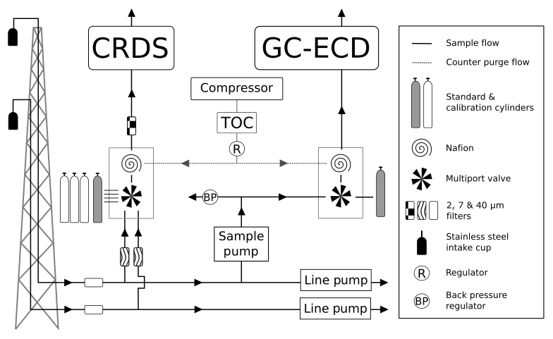
Figure 2A generalized schematic showing the initial Bilsdale and Heathfield site set-up of the cavity ring-down spectrometer (CRDS) and the gas chromatograph–electron capture detector (GC–ECD) including the dry gas generator (TOC) and back pressure regulator (BP). Note that Bilsdale has three inlets, while Heathfield has only two as shown here. The Nafion® drying system located downstream of the CRDS multiport valve was removed at both sites in 2015. Black arrows and lines show the direction of sample, standard and calibration gas flow. Grey dashed lines and arrows show the flow path of the Nafion® counter purge gas.
2.3.2 CRDS
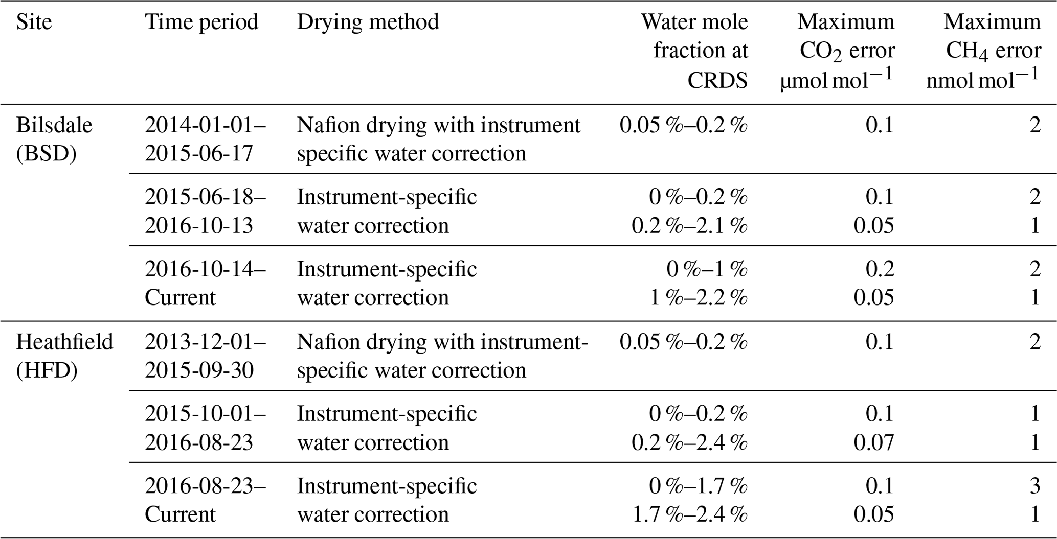
In an attempt to minimize the water correction required for dry mole fraction CRDS measurements, CRDS samples were initially dried using a Nafion® dryer in an identical manner to those of the GC–ECD. When functioning correctly this drying method resulted in air samples with water mole fractions between 0.05 % and 0.2 % H2O depending on the original moisture content of the air and temperature. However, at Bilsdale, due to problems with the TOC gas generator and the tubing initially installed at the site, the Nafion® was not drying optimally and significant periods of 2014 had far higher moisture contents (Fig. S1).
Due to concerns that the mole fraction gradient between the sample and the Nafion® counter purge might lead to CO2 transport across the Nafion® membrane and difficulties associated with maintaining a complex drying system at remote locations, this drying approach was discontinued. The CRDS Nafion® drying systems were removed on 30 September and 17 June 2015 at BSD and HFD respectively. Following this, undried air was analysed and the data post-corrected with an instrument-specific water correction. Plots of the water content of all air samples along with the comparisons of the diurnal and seasonal cycles in sample moisture content can be found in the Supplement (Figs. S1 and S2).
2.3.3 Composition of the counter purge dry air stream
The drying technique implemented in this study uses a Nafion® dryer which relies on a dry counter purge air stream. Measurements of these air streams were made at BSD, HFD and the University of Bristol (UoB) laboratory using the respective sites' CRDS instrumentation. All counter purge streams showed mole fractions of CO2 < 0.3 µmol mol−1, CH4 < 2 nmol mol−1 CO < 12 nmol mol−1 and H2O < 0.01 % (Fig. S3). All these zero-air streams have CO2 and CH4 mole fractions far lower than the 2015 mean global concentrations, 400.99 µmol mol−1 CO2 and 1840 nmol mol−1 CH4 (Dlugokencky and Tans, 2015; Dlugokencky, 2015). Similarly, the zero-air CO mole fraction is significantly lower than the minimum CO mole fractions typically observed at the HFD and BSD sites (∼60 nmol mol−1). As such there is a clear and sizable partial pressure difference across the Nafion® membrane for all three species.
2.3.4 Calculating instrument-specific water corrections
Motivated by the possibility of CO2 transport across the Nafion® membrane, the decision was made to measure wet samples and correct using an instrument-specific water correction. These corrections were determined in the field by conducting a droplet test, similar to those described in Rella et al. (2013). In this test, air from a cylinder of dry (< 0.002 % H2O) natural air was humidified and the change in CO2 and CH4 mole fractions with water content examined. In brief, a 1.5 m length of 3∕8 in. Synflex Dekabon metal–plastic composite tubing (Eaton, USA) was introduced between the standard cylinder outlet and the CRDS intake. Distilled water (0.7 mL) was injected through a septum located on a T-piece fixed on the “cylinder end” of the Dekabon tubing (see Fig. S4 for flow diagram). This water evaporated into the sample stream, with the H2O mole fraction typically peaking at up to 4.5 % (dependent on room temperature) before decreasing to pre-injection concentrations. The effect of this changing H2O concentration on the raw (without the inbuilt H2O correction) CO2 and CH4 concentrations was then observed. The experiment was repeated in at least triplicate annually.
Data collected in the first 5 min immediately following the injection, the typical line equilibration period, were excluded from the fit. This avoids using data adversely affected by the effect of rapid changes in H2O content on the cell pressure sensor, as identified by Reum et al. (2019) and the erroneous post-injection CO2 enhancement identified by Rella et al. (2013). Again, due to cell pressure sensor concerns, data points with minute-mean H2O standard deviations > 0.5 % H2O were excluded. This 5 min cut-off reduced the maximum H2O value included in the fit to 4 % H2O.
A water correction was then determined from a fit between the mean wet ∕ dry ratio and the H2O of the droplet test data and the equation given by Rella (2010). Here we defined dry data as any data with H2O < 0.003 %, as measured by the CRDS, and the remaining data as wet. We use minute-mean uncorrected CRDS CO2 and CH4 data for this analysis, that is, minute-averaged data from the “co2_wet” and “ch4_wet” columns of the raw Picarro data files along with data from the “h2o” column. These H2O data, unlike the “h2o_reported” data, have been corrected for spectral self-broadening as detailed in Rella (2010). A similar analysis was conducted for CO. However, this used the “co” data, which have water vapour and line interference corrections applied to it. The raw co values (i.e. “co_wet”) are not provided in the CRDS output files.
Table 1Instrument-specific water corrections for the Bilsdale (BSD), Heathfield (HFD) and University of Bristol (UoB) CRDS instruments. The parameters shown are the mean ± the 95 % confidence interval of tests repeated in triplicate. Water corrections labelled high and low were determined using an above-ambient and below-ambient mole fraction cylinder respectively, while the rest were determined using an ambient mole fraction cylinder. The mean residual along with the interquartile range of the residuals are included.

* The fitted parameter and 1σ2 of a single test due to a leak in the septum.
The fit was conducted using orthogonal distance regression weighted by both the minute-mean standard deviation of the H2O and gas of interest (CO2 or CH4). The resulting correction parameters are shown in Table 1. These corrections were then applied to minute-mean observational data through the GCWerks software completely bypassing the built-in CO2 and CH4 water corrections.
As Picarro analysers are not calibrated for H2O measurements when measuring dry air, they often show different positive or negative values close to zero. These “zero-water” values were 0.00001 %, −0.0003 % and −0.002 % for the Bilsdale, Heathfield and University of Bristol laboratory instruments respectively. These values were determined using measurements of cylinders of dry air where the first 120 min was ignored and the zero-water value calculated as the mean H2O of the subsequent data (> 60 min).
2.3.5 Temporal stability and mole fraction dependence of instrument-specific water corrections
The typical temporal stability and mole fraction dependence of the CRDS water correction were examined using a laboratory-based CRDS (G2301, Picarro Inc., USA; CO2, CH4 and H2O series). Here the water correction was determined using the droplet experiment, as described in Sect. 2.3.4. The mid-term and short-term stabilities were examined by repeating the experiment approximately weekly over a 3-month period and daily for a 5 d period using a cylinder of dried ambient mole fraction air. A set of instrument-specific water corrections was also determined in triplicate, using dried sub- and above-ambient CO2 and CH4 mole fraction cylinders. As this instrument was not able to measure CO, the effect of CO mole fraction on the CRDS instrument-specific water correction is not addressed in this paper.
2.3.6 Assessing the CRDS water correction
The accuracy of the CRDS water correction determined through the water droplet test, as described in Sect. 2.3.4, was assessed through a series of simple dew point generator (DPG; Li-cor LI-610 portable dew point generator, USA) experiments. Here, dry air from four cylinders with varying CO2 and CH4 mole fractions (Table 2) was humidified to a range of set dew points between 2.5 and 30 ∘C (0.6 % to 3.5 % H2O) and measured, with and without cryogenic drying, at the University of Bristol (UoB) laboratory using the same Picarro G2301 CRDS used in Sect. 2.3.5 and 2.3.7. Cylinder delivery pressure was controlled using single-stage high-purity stainless steel Parker Veriflo regulators (95930S4PV3304, Parker Balston, USA) or TESCOM regulators (64-2640KA411, Tescom Europe).
In brief, the output of the cylinder regulator was plumbed to the input of the DPG. A T-piece connected prior to the DPG input vented any excess gas via a flowmeter (F1, Fig. 3a) ensuring that the DPG input remained at close to ambient atmospheric pressure throughout the experiment. The output of the DPG passed through a second T-piece with the overflow outlet also connected to a flowmeter (F2) to ensure that the CRDS input pressure remained near ambient. A third flowmeter (F3) was placed on the outflow of the Nafion counter purge. Flowmeters F1 and F2 had a range of 0.1–1 L min−1 (VAF-G1-05M-1, Swagelok, UK) while F3 had a smaller flow range 0.1–0.5 L min−1 (FR2A12BVBN-CP, Cole-Palmer, USA). Typical output flows were 0.1, 0.3 and 0.3 L min−1 for F1, F2 and F3 respectively. After F2 the sample flow was further split using a T-piece, with half the flow passing through a cryogenic water trap before reaching a four-port two-position valve, V1 (EUDA-2C6UWEPH, VICI AG International, Valco Instruments Co. Inc., Switzerland, actually a six-port valve configured as a four-port valve). The other half bypassed the water trap and connected directly to V1. One of the outputs of V1 went via the Nafion to a second identical valve, V2, while the second output went directly to V2. The first output of V2 connected directly to the input of the CRDS while the second connected to a pump (Picarro vacuum pump S/N PB2K966-A) set to a flow rate matching that of the CRDS (0.3 L min−1) to ensure uniform flow through both branches of the system. These valves were controlled manually using a Valco electronic controller and universal actuator.
The cryogenic water trap consisted of a coil of 1∕4 in. diameter (I.D. 3.36 mm) stainless steel tubing immersed in a Dewar of silicone oil (Thermo Haake SIL 100, Thermo Fisher Scientific, USA). The silicone oil was cooled using an immersion probe (CC-65, NESLAB) to less than −50 ∘C. Other than the water trap and two short sections (< 10 cm) of 1∕4 in. (O.D.) plastic tubing immediately prior to and post the DPG, 1∕16 in. stainless steel tubing was used throughout the system. Due to the air output and input connections of the DPG, the use of the plastic tubing was unavoidable.
Table 2The cylinders used during the dew point generator CRDS water correction, Nafion® counter purge and UoB instrument-specific water tests. Most measurements were made in-house and only corrected for linear drift against a standard calibrated at WCC-EMPA, Dübendorf, Switzerland, and hence are simply indicative of the expected mole fractions. Those marked * were calibrated at GasLab MPI-BGC, Jena, Germany, and linked to the WMO x2007 CO2 and x2004A CH4 scales.
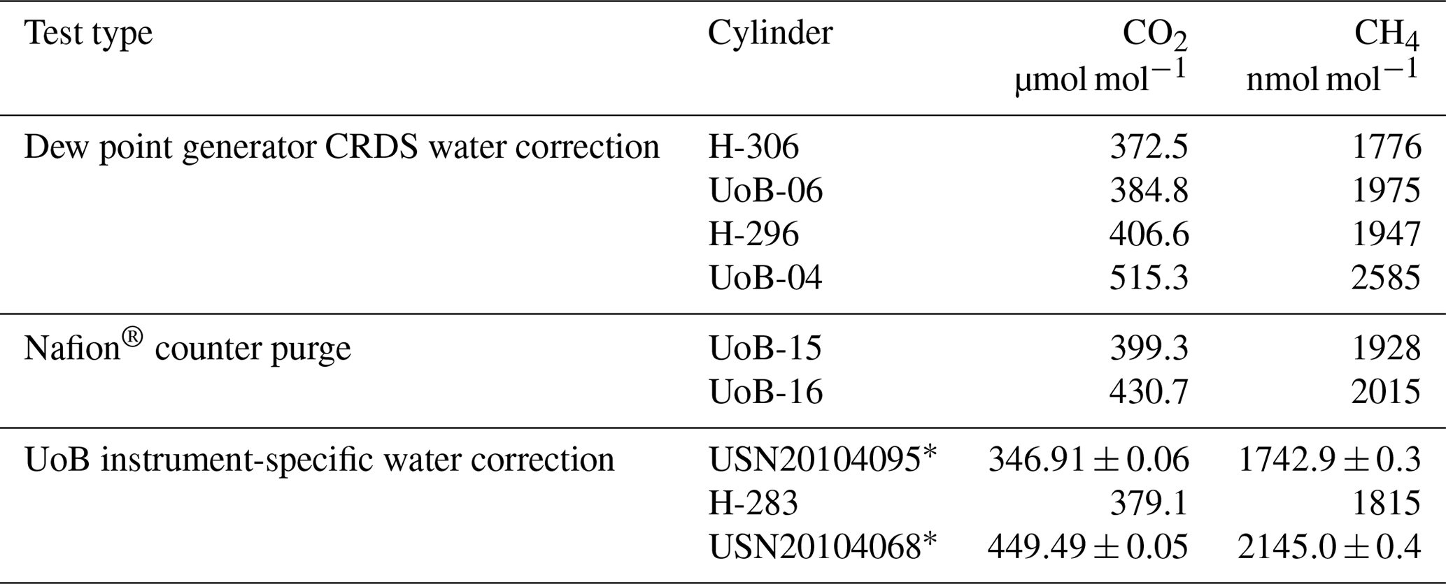
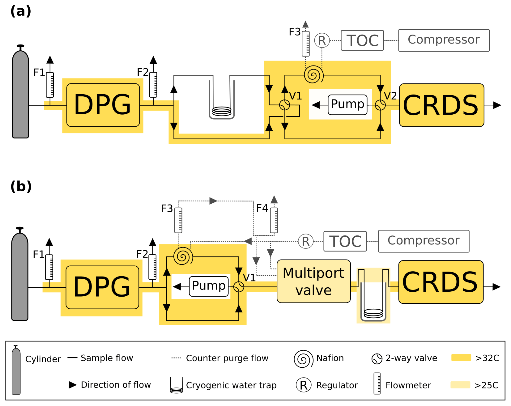
Figure 3A schematic of the humidification system used in the (a) CRDS water correction assessment and (b) Nafion® counter purge experiment including the dew point generator (DPG). Here the TOC is the dry gas generator. The black arrows and lines show the direction of sample gas flow. Grey dashed lines and arrows show the flow path of the Nafion® counter purge gas. Heated zones are shown in yellow.
The experiment was conducted in a temperature-controlled laboratory at 19 ∘C, and thus at temperatures lower than a number of the dew points used within the experiment. Hence, in order to avoid condensation forming on the walls of the tubing all components of the system between the cylinder, excluding the water trap, and the outputs of V2 were contained within a chamber heated to > 32 ∘C. Tubing between the heated chamber and the input of the CRDS was also heated with heating tape to > 32 ∘C while the internal temperature of the CRDS was > 32 ∘C throughout the experiment.
Multiple measurement blocks of each sample treatment were conducted after a lengthy initial stabilization period. This period allowed for the establishment of equilibrium between the water in the condenser block of the DPG and the sample gas and lasted at least 2 h (sometimes up to 5 h). The treatment blocks varied in length depending on the time required for the concentration to stabilize. At least 15 min of data was collected after the concentration stabilized.
It is important to note that the DPG was not calibrated but the H2O concentration was measured directly by the CRDS during the undried experiments. These values were used as the reference H2O concentration in all calculations and plots.
Flow rates, cylinder pressure, chamber temperature and H2O trap temperature were manually logged after each valve position change and when the water trap was inserted into the silicone oil bath.
2.3.7 Quantifying CO2 and CH4 cross-membrane transport using measurements of the counter purge gas
Experimental details
An experiment was designed to observe gas exchange across the Nafion® membrane by measuring the counter purge gas before (CPin) and after (CPout) the Nafion® while varying the water and CO2 and CH4 content of the sample gas stream.
In this experiment, a system (Fig. 3b) was constructed allowing the controlled humidification, using a DPG, of two high-pressure cylinders, one of dry near-ambient and one above-ambient CO2 and CH4 mole fractions (Table 2; UoB-15 and UoB-16). These humidified air samples were measured using the UoB laboratory Picarro CRDS as used in Sect. 2.3.5 and 2.3.6. This experimental set-up is very similar to that described in Sect. 2.3.6. However, the range of dew points examined was slightly smaller (between 5 and 25 ∘C) equating to water contents of between 0.786±0.001 and 2.883±0.003 % H2O. This limitation was introduced as the multiport valve was heated to only > 25 ∘C.
Other differences include the placement of the Nafion®, water trap and the addition of a multiport valve. In this experiment the humidified cylinder air exiting the third T-piece is split with half passing through the Nafion® before reaching a four-port two-position valve, V1 (EUDA-2C6UWEPH, VICI AG International, Valco Instruments Co. Inc., Switzerland, actually a six-port valve configured as a four-port valve). The other half bypassed the Nafion® and connected directly to V1. The first output of V1 connected to a multiport valve (EUTA-CSD10MWEPH, VICI AG International, Valco Instruments Co. Inc., Switzerland) while the second connected to a pump (Picarro vacuum pump S/N PB2K966-A) set to a flow rate matching that of the CRDS (0.3 L min−1) to ensure uniform flow through both branches of the system. The V1 valve was controlled manually using a Valco electronic controller and universal actuator while the multiport valve was controlled by the GCWerks software. The output of the multiport valve was connected to the CRDS via the cryogenic water trap (See Sect. 2.3.6).
Counter purge air, both before (CPin) and after (CPout) the Nafion®, was also sampled using the multiport valve. To do this a T-piece was placed on the counter purge tubing prior to the Nafion® connecting to the multiport valve while a second T-piece located after the Nafion® was again connected to the multiport valve. Two flowmeters, F3 and F4, were used to monitor the counter purge flow. Flowmeter F3 was placed on the outflow of the Nafion® counter purge prior to the T-piece while a second F4 was connected to one output branch of the T-piece. These flowmeters had a flow range of 0.1–0.5 L min−1 (FR2A12BVBN-CP, Cole-Palmer, USA). When not sampling the counter purge, F3 and F4 had flow rates of 0.4 L min−1; when sampling CPout the F4 flow rate dropped to 0.2 L min−1.
As the reliability of CRDS water correction was also under investigation, it was important to isolate the effect of the Nafion® from that of the CRDS water correction. To do this the experiment was conducted in three stages (see Fig. S5). Firstly, the H2O content of the DPG humidified sample stream was allowed to stabilize (Fig. S5 purple). A stable water content was defined as one where the standard deviation of the minute-mean values was < 0.003 % H2O for a 15 min period. During this period the H2O trap remained out of the Dewar of silicone oil and the CRDS measured an undried, Nafion®-bypassed sample, while the secondary pump maintained the flow of DPG sample through the Nafion®. After this criterion was reached the second stage was commenced. Here the H2O trap was inserted into the silicone oil and the water content monitored until 10 min of dry air (defined as < 0.002 % H2O) was obtained (Fig. S5 grey). Together these two stages took typically 2 to 3 h to complete – allowing the Nafion® time to equilibrate while ensuring that the H2O trap was drying the sample and the DPG had reached the required set point. At the start of the third stage, the multiport valve was used to switch between the CPin or CPout flows, measuring each for repeated 20 min blocks (n > 3) at each dew point (see Fig. S5 red and blue). The H2O trap remained inserted in the silicone oil throughout the third stage. The experiment was also repeated with the DPG excluded and the cylinder of dried air measured directly, with a water content of < 0.0001 % equating to a dew point of < −70 ∘C.
Data processing
All CO2 and CH4 data were corrected using the instrument-specific water correction (Sect. 2.3.4). Minute-mean values of all data were calculated from the raw 0.4 Hz data and exported from the GCWerks software. Data processing was completed using code written using the Anaconda distribution of the Python programming language (Python Software Foundation, 2017; van Rossum, 1995) and a variety of standard packages including NumPy1.11.1 (van der Walt et al., 2011), SciPy 0.18.1 (Jones et al., 2001) and Matplotlib 2.0.2 (Hunter, 2007).
The counter purge measurements made during the humidification experiments represent a combination of effects.
Here, Truecp is the true mole fraction of the counter purge gas, NX% is the effect of the Nafion® at X % H2O in the sample stream, and X % is the water content of the sample gas before the Nafion®.
Hence the difference between the mean of CPin and the mean of CPout represents both any transport of CO2 (or CH4) through the Nafion® membrane and the effect of the water correction at low humidities.
In order to remove any valve switching or line equilibration effects the first 5 min of data of each sample period was discarded and the mean of the final 15 min period of each sample type at each dew point was calculated. The uncertainty of this mean was determined as the 95 % confidence interval based on the larger of either the standard deviation of the minute means or average of the standard deviations of the minute means. Examples of the raw data collected during the experiment are given in Fig. S5. As the experiment was subject to a small temporal drift, the mean CPin values were linearly interpolated and the CPout–CPin difference calculated as the difference between the CPout and time-adjusted CPin values and the uncertainty estimated as the combined uncertainty of the CPin and CPout values.
2.3.8 Key experimental assumptions
While experiments 2.3.5, 2.3.6 and 2.3.7 were designed to isolate key processes, other possible sources of error or bias may exist. These include adsorption and desorption effects within the regulator and walls of the tubing, gas solubility within the condenser of the dew point generator, and instrumental drift.
Regulator and tubing adsorption and desorption effects have been previously examined by Christoph Zellweger and Martin Steinbacher (2017, personal communication). They found that for Parker Veriflo regulators, as used in this experiment, the effects can be quite large, up to 0.5 µmol mol−1 CO2 or 2 nmol mol−1 CH4, but that these effects were only evident at flow rates < 250 mL min−1 and after significant periods of stagnation (15 h). Considering the high flow rates (> 1 L min−1) and long flushing times (2 to 3 h) used in our experiment, it is highly unlikely that regulator effects would make a significant impact on the results.
As discussed earlier, a lengthy equilibration period was used at the start of each DPG run and following any change in DPG set point. This was to account for the dissolution of sample gas, in particular CO2, in the DPG water chamber. After this initial equilibrium period there were no rapid changes in the CO2 mole fraction with only a slow drift, apparent in the data. CRDS instrumental drift is also typically very small and slow. For the UoB CRDS instrument, long-term measurements of target-style standard cylinders have shown the drift to be < 0.001 µmol mol−1 d−1 CO2 and < 0.03 nmol mol−1 d−1 CH4. These drift rates are at least an order of magnitude smaller than the mole fraction differences observed in this study.
Although small, any time-dependent drifts were accounted for by temporally interpolating between each block of data. Also key to the design of this experiment is the examination of differences between two very similar mole fractions rather than absolute mole fractions. As such, any systematic errors that might drive a systematic offset cancel out and any mole-fraction-dependent biases are minimized.
Table 3CRDS calibration and standard cylinder mole fractions and usage start dates for the Heathfield (HFD) and Bilsdale (BDS) sites. Where available the mole fractions measured prior to and after deployment are given. Reported mole fractions from the WCC-EMPA, Dübendorf, Switzerland, are given as mean ± uncertainty. * Mole fraction measurements from GasLab MPI-BGC, Jena, Germany, are given as mean ±1σ.
2.3.9 Calibration and traceability
Calibration procedures for both the CRDS and GC–ECD are as described in detail in Stanley et al. (2018). In brief, CRDS measurements are calibrated using a close-to-ambient standard (“working tank”) and a set of three calibration cylinders, which span the typical ambient range (Table 3). Only a small number of elevated observations, < 0.4 % of the CO2 and < 1.5 % of the CH4 minute-mean observations, were outside the range of the calibration cylinders. However, a much higher proportion of the CO observations were outside the range of the calibration suites used at the sites, 28 % at BSD and 43 % at HFD, with the majority of these data points (> 98 %) below the lowest calibration cylinder.
Assigning mole fractions to values outside the range of the calibration suite will increase the error. The magnitude of this error will depend on the magnitude of the mole fraction difference between the closest calibration cylinder and the sample. This error has been estimated using measurements made at the Heathfield site of cylinders of known CO mole fractions, 6 and 57 nmol mol−1 CO below the lowest calibration cylinder. These show a percentage error of 2.41 % and 3.09 % respectively. A similar assessment of the error associated with samples above the highest calibration standard was made using cylinders 87 and 686 nmol mol−1 CO above the highest calibration standard. These correspond to percentage errors of 2.98 % and 2.56 % respectively. As all the minute-mean CO measurements below the calibration range are within 57 nmol mol−1 of the lowest calibration cylinder and the vast majority of minute-mean CO measurements above the calibration range are within 686 nmol mol−1 of the highest calibration cylinder (99 %), we expect that this error would typically be < 3 %.
Daily 20 min long measurements of the ambient standard are used to account for any linear drift, while monthly measurements of the calibration suite are used to characterize the nonlinear instrumental response. This calibration procedure is controlled by the GCWerks software and allows near-real-time examination of calibrated data. During the period that the Nafion® drying system was used these standards were partially humidified as they passed through the wet Nafion® dryer. The level of humidification is dependent on that of the air samples measured prior to the standard. The moisture content of the standard closely tracks that of the air samples with variations in the humidity of the samples clearly reproduced in the standard (Fig. S1). However, the moisture content of the standard is generally slightly lower. On average the standard has a mean moisture content 88 % that of the average of the 30 min of air sample either side of the standard (on average 0.02 % H2O lower). The moisture content of the standard also decreases slightly during the 20 min measurement period as the dry standard air dries out the Nafion® membrane. The size of this decrease is dependent on the moisture content of the prior air samples with larger decreases during the more humid times of the year. As a worst-case example, the change in the water content of the Heathfield standard during each run of August 2014 is shown in Fig. S6. This shows a maximum drift of 0.07 % H2O equating to 30 % of the mean moisture content of air observations collected 30 min either side of the standard
In contrast, due to the time taken to take replicate measurements of the calibration cylinders (at least 240 min) only the first 20 min measurement block of each calibration cylinder is significantly humidified. with the water content of the calibration measurement dropping rapidly to < 0.02 % H2O (10 % to 20 % of the typical ambient air measurements). However, the exact level of humidification varies with ambient humidity and temperature. As such, in an effort to maintain consistency between calibration runs all runs with > 0.02 % H2O were excluded from analysis.
All CRDS standards and calibration gases are composed of natural air, some spiked or diluted with scrubbed natural air (TOC gas generator, model no. 78-40-220, Parker Balston, USA), to achieve the required concentrations of CO2, CH4 and CO. All standard cylinders were filled at Mace Head with well-mixed Northern Hemisphere air. The cylinder spiking and filling techniques of the calibration cylinders varied. The Heathfield calibration suite and the second Bilsdale calibration suite were filled at GasLab MPI-BGC Jena and consisted of natural air spiked using a combination of pure CO2 and a commercial mixture of 2.5 % CH4 and 0.5 % CO in synthetic air. The “high” calibration cylinder of the first calibration suite used at the Bilsdale site was filled with peak-hour ambient air at EMPA, Dübendorf, Switzerland, while the “low” and “mid” cylinders were based on Mace Head air. In the case of the low cylinder this was diluted with scrubbed natural air. Using natural-air-based calibration and standard gases removes any pressure broadening effects inherent in the use of non-matrix-matched artificial standards (Nara et al., 2012). As the CRDS is an isotopologue-specific method filling the cylinders in such a manner ensures that the isotopic composition was as close to those of the sampled air as possible. The effect of an isotopic mismatch between the calibration standards and the sample has been examined in detail by Flores et al. (2017), Griffith (2018) and Tans et al. (2017). With Griffith (2018) showing that, for a sample of 400 µmol mol−1 CO2 and 2000 nmol mol−1 CH4, the error will range between 0.001 and 0.155 µmol mol−1 CO2 and 0.1–0.7 nmol mol−1 CH4 depending on the magnitude of the sample-to-standard mismatch. Based on this we expect a worst-case scenario estimate of the error associated with our typical ambient measurements to be < 0.04 % for both CO2 and CH4.
GC–ECD measurements are made relative to a natural air standard of known N2O and SF6 concentration. This standard is measured hourly and used to linearly correct the samples (Table 4). The instrumental nonlinearity response was characterized prior to deployment by dynamically diluting a high concentration standard with zero air and was repeated in the field at the BSD site on 30 September 2015. This approach, dynamic dilution, has a history of use in similar field locations (Hammer et al., 2008) and is able to generate multiple calibration points using just two cylinders. This greatly reduces the number of cylinders needed, a key concern for space-limited locations like BSD and HFD. An assessment of the uncertainty associated with this nonlinearity approach will be included in a future paper currently in preparation. However, previous studies (Hall et al., 2011; van der Laan et al., 2009; Hammer et al., 2008) have found the ECD response to be extremely stable over time and very linear for both SF6 and N2O in the mole fraction range typical of the HFD and BSD stations. As such, we expect the uncertainty of the nonlinearity correction to be very small.
Table 4GC–ECD standard cylinder mole fractions and usage start dates.
GC–ECD and CRDS standards and calibration cylinders were, where possible, calibrated both before and after deployment at the sites. If these two measurements agreed then a mean mole fraction was used, otherwise a linearly drift-corrected mole fraction was used. The CRDS cylinders were calibrated through WMO linked calibration centres (either WCC-EMPA, Dübendorf, Switzerland, or GasLab MPI-BGC, MPI, Jena, Germany). This ties the ambient measurements to the WMO CO2 x2007 (Zhao and Tans, 2006), CH4 x2004A (Dlugokencky et al., 2005) and CO x2014A (Novelli et al., 1991) scales. The calibration of the GC–ECD standards was conducted at either the AGAGE Mace Head laboratory or the University of Bristol laboratory and is reported here on the recently released SIO-16 N2O scale and the SIO SF6 scale. Most cylinders were or will be calibrated before and after deployment and the mean of the two values used. Some cylinders, due to logistical constraints were only calibrated once (Table 4).
2.3.10 Instrument short-term precision and long-term repeatability
The short-term (1 min) precision of the CRDS data was determined as the mean of the standard deviations of the 1 min mean data. This was calculated from measurements of the standard cylinder and the calibration suite allowing the relationship between CO2, CH4 and CO mole fractions and short-term precision to be examined. This analysis included 18 cylinders covering a wide range of mole fractions (Table 3).
The mean absolute short-term precision for all cylinders was consistent between the two sites across all three gases. At BSD the short-term precision was 0.024 µmol mol−1 CO2, 0.18 nmol mol−1 CH4 and 4.2 nmol mol−1 CO while at HFD it was 0.021 µmol mol−1 CO2, 0.22 nmol mol−1 CH4 and 6 nmol mol−1 CO. Both sites showed a small trend with the mean absolute precision worsening with increasing CO2 and CH4 mole fractions. However, this was not observed in the relative precision, which remained unchanged at ∼0.005 % for CO2 and ∼0.01 % for CH4. This was not the case for CO, where the relative precision improved with increasing mole fraction from ∼4 % at CO < 100 nmol mol−1 to < 1.5 % at CO > 250 nmol mol−1. We suspect that this tendency is inherent in the spectroscopic approach as the CO peak measured by the Picarro CRDS is much smaller than those of CO2 and CH4 (Chen et al., 2013) and hence more susceptible to noise in the baseline, particularly at low mole fractions.
The long-term reproducibility of a 20 min mean was estimated as the mean standard deviation of the daily 20 min measurements of the standard cylinders used at each site. A total of eight standard cylinders have been used in succession at the two sites with the usage periods and CO2, CH4 and CO mole fractions listed in Table 3. Like short-term precision, mean long-term reproducibility (calculated over a period of approximately a year) is consistent between the two sites, 0.018 and 0.013 µmol mol−1 CO2, 0.20 and 0.20 nmol mol−1 CH4, and 1.1 and 1.7 nmol mol−1 CO at BSD and HFD respectively.
Repeatability of individual injections on the GC instruments was calculated as the standard deviation of the hourly standard injection. These were found to be < 0.3 nmol mol−1 and < 0.05 pmol mol−1 for N2O and SF6 respectively, and did not differ between the two sites.
2.4 Data analysis
2.4.1 Data quality control
A three-stage data flagging and quality control system was used for the HFD and BSD data. Initially, automated flags based on the stability of key parameters including cell temperature and pressure and instrument cycle time (the time taken to collect and process each measurement) were applied. Here, data with a cycle time > 8 s were filtered out along with any data with cell temperature outside the range of 45±0.02 ∘C or cell pressure outside 18.67±0.01 kPa. Secondly, a daily manual examination of the GC chromatograms and key GC–CRDS parameter values of each site was performed. Data points were flagged if instrument parameters varied beyond thresholds determined to reduce their accuracy and a reason for the removal was logged. Finally, all sites were reviewed simultaneously and the mixing ratio of the same gas from each site is overlaid to look for differences between sites. Any significant differences between the background values at each site were investigated by examining key instrumental parameters, calibration pathways and 4-hourly air mass history maps to ensure that these differences represent true signals rather than instrumental or calibration-driven artefacts. The hourly air mass history maps were produced using the Numerical Atmospheric dispersion Modelling Environment (NAME) Lagrangian dispersion model (Manning et al., 2011).
2.4.2 Statistical processing, baseline fitting and seasonal cycles
The long-term trend in mole fraction at each site was estimated as the mean linear trend in the minute-mean data over the period 2014–2017, inclusive. Seasonal and diurnal trends in the data were assessed using monthly and hour-of-day means of trimmed detrended minute-mean data developed using the Python numpy package. Here the long-term trend was removed by using a least-squares fit between a quadratic and the minute-mean data. The data for each hour (or month for the seasonal plots) were trimmed following the approach of Satar et al. (2016), who removed the highest and lowest 5 % of all data points.
3.1 CO2, CH4 and CO key features
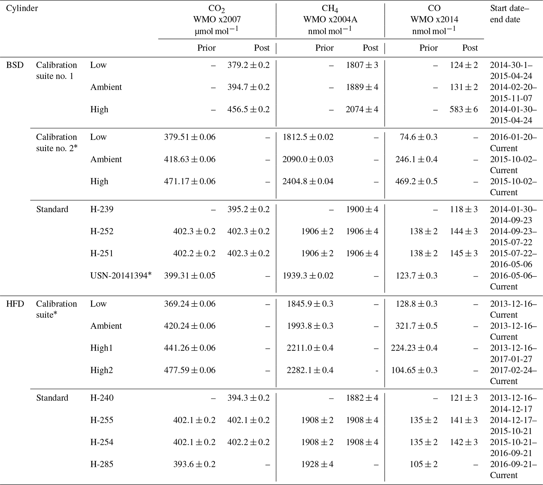
The minute-mean CO2 observations range between a low of 379.50 and a high of 497.48 µmol mol−1 CO2 at Heathfield and 379.77 and 587.17 µmol mol−1 CO2 at Bilsdale. High CO2 mole fractions observed at BSD are generally higher than those of the HFD site (Figs. 4a and 5a). The high-mole-fraction events observed at BSD are generally sporadic – lasting only a couple of hours – and appear as a brief pulse relative to the normal diurnal cycle, a pattern indicative of a nearby point source. Considering BSD is remote from large conurbations, measured signals are expected to be dominated by biogenic sources. In this instance, we suspect high-mole-fraction events at BSD are due to local heather (Calluna vulgaris) burning. These CO2 events also typically coincide with periods of elevated CH4 and CO, again suggesting a biomass burning source. In contrast, events that do not show corresponding high CO and CH4 mole fractions tend to occur in the higher two intakes. As such, they are likely to be driven by more remote CO2 sources, for example power plants.
Figure 4Minute-mean (a) CO2, (b) CH4 and (c) CO and 10 min discrete (d) N2O and (e) SF6 observations at the Bilsdale site for the 42 m (blue), 108 m (green) and 248 m (purple) intake heights.
HFD is located in southern England, just south of London (Fig. 1). Here, high CO2 events are typically longer – 2 to 3 d – and coincide with elevated CH4, CO, N2O and SF6. Rather than appearing as peaks superimposed on a background value, these periods have a positive shift in the entire diurnal cycle. Air histories, based on the output of the NAME Lagrangian dispersion model, outlined in Manning et al. (2011), for these periods of elevated CO2 typically show the source of the air to be from over London or Europe.
Both sites show a clear relationship between CO2 mole fraction and intake height with the lowest height generally having the most elevated mole fractions, followed by the higher heights (Figs. 4a and 5a). This trend, also apparent for CH4 and CO (Figs. 4b and c and 5b and c), is typical of tall tower measurements and is driven by proximity to surface sources (Bakwin et al., 1998; Winderlich et al., 2010; Satar et al., 2016). This gradient in CO2 and CH4 mole fraction is most apparent in the warmer seasons and during the early hours of the morning (Fig. 6a, b, c and d) when the boundary layer is the lowest, a trend observed previously by Winderlich et al. (2010). A reversal of this gradient, with lower heights having lower CO2 mole fractions, occurs in the middle of the day (Fig. 6a and b). As described in Satar et al. (2016) this decrease in near-surface CO2 is most likely driven by local photosynthetic activity. Interestingly, this trend is also apparent in spring, summer and autumn CH4 mole fractions at BSD (Fig. 6c) but not HFD (Fig. 6d). This suggests a midday sink of CH4 local to BSD but not HFD. Considering that BSD is located high in the Yorkshire moors (379.1 m a.s.l) while HFD is located in a lower agricultural region (157.3 m a.s.l), a large difference in soil moisture, and therefore methanotrophic activity (Topp and Pattey, 1997), between the two sites is possible.
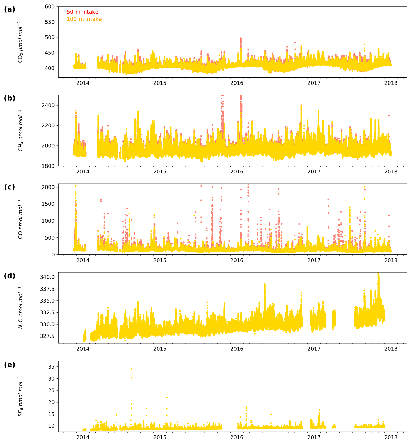
Figure 5Minute-mean (a) CO2, (b) CH4 and (e) CO and 10 min discrete (d) N2O and (e) SF6 observations at the Heathfield site for the 50 m (red) and 100 m (yellow) intake heights.
Interestingly, Winderlich et al. (2010) suggest that their ability to observe gradients on an hourly timeframe is only revealed due to their use of buffer volumes and fast switching (every 3 min). In contrast, the measurements presented here, made without buffer volumes and at a much lower switching rate, were also able to identify gradients between the heights (Fig. S7). This suggests that the use of buffer volumes and fast switching is not required in order to observe these trends.
The timings and magnitude of the HFD and BSD seasonal cycles are similar, with CO2 mole fractions highest in the colder months and lowest during the Northern Hemisphere summer (Fig. 7a and b). Although both sites are located in areas consisting of predominantly agricultural space or native vegetation, the HFD site is more urbanized. This appears to be reflected in more elevated CO2 and CO events in October, November and December relative to the BSD site (Fig. 6a and b and e and f), suggesting that the HFD site is more sensitive to fossil fuel emissions.
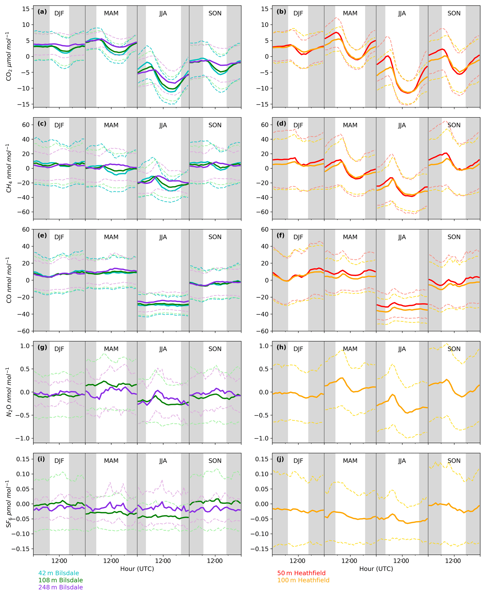
Figure 6Mean diurnal cycle by season of detrended hourly mean values for (a, b) CO2, (c, d) CH4, (e, f) CO, (g, h) N2O and (i, j) SF6 of the Bilsdale 42 m (blue), 108 m (green) and 248 m (purple) and Heathfield 50 m (red) and 100 m (yellow) intake heights. Dashed lines are the standard deviation.
As with the seasonal cycle, the shape of the CO2 diurnal cycle is similar at both sites, with mole fractions peaking near sunrise and the lowest CO2 mole fractions observed in the late afternoon (Fig. 6a and b). Again, the amplitude of these cycles varies between the sites, with HFD, the more anthropogenically influenced site, typically showing a higher maximum in the early morning than BSD.
Although there is a very large range in the minute-mean CH4 observations, 1841 to 3065 nmol mol−1 at BSD and 1843 to 3877 nmol mol−1 at HFD, > 99.99 % of measurements are less than 2400 nmol mol−1 CH4, with only six events in the combined record exceeding this threshold. These events have been clipped from the data shown in Figs. 4b and 5b for ease of viewing. Like CO2, the CH4 observations show seasonal cycles with mole fractions being the highest in the winter months and the lowest in midsummer (Fig. 7c and d). A small CH4 diurnal cycle peak occurs in the morning usually 1 to 2 h after sunrise (this is after the CO2 maximum) and then dips in the mid-afternoon (Fig. 6c and d). The CH4 diurnal cycle is also more pronounced and smoother in the HFD data and evident throughout the year, whereas the BSD cycle is only strongly apparent in the summer months. This could be linked to differences in the relative magnitude of key local sources and sinks of CH4 between the two sites.
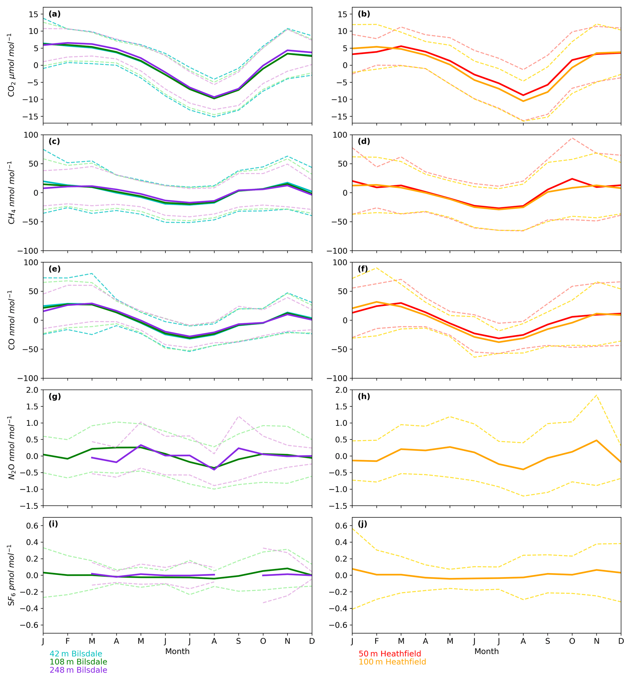
Figure 7Mean seasonal cycle of detrended hourly mean values for (a, b) CO2, (c, d) CH4, (e, f) CO, (g, h) N2O and (i, j) SF6 of the Bilsdale 42 m (blue), 108 m (green) and 248 m (purple) and Heathfield 50 m (red) and 100 m (yellow) intake heights. Dashed lines are the standard deviation.
Of the five gases measured at HFD and BSD, CO is the only gas to show a decrease in mole fraction between 2013 and 2017, roughly −7 nmol mol−1 yr−1. In contrast, the CO2 and CH4 data increase by 2–3 µmol mol−1 yr−1 and 5–9 nmol mol−1 yr−1 respectively, varying with the intake height. These agree well with the ∼2 µmol CO2 mol−1 yr−1 and ∼8 nmol CH4 mol−1 yr−1 trends observed at Mace Head (MHD, 53.327∘ N, 9.904∘ W, Fig. 1), a remote site within the UK DECC network located on the west coast of Ireland. However, the CO data collected at MHD are not on the NOAA x2014 CO calibration scale, making direct comparisons between growth rates difficult to interpret.
While the range of minute-mean CO mole fractions was significantly larger at BSD, 63 to 9500 nmol mol−1 than HFD, 60 to 4850 nmol mol−1, the high CO values observed at BSD were relatively rare. This is reflected in the smaller spread of the BSD data compared with the HFD data (Fig. 7e and f).
3.2 N2O and SF6 key features
The range of N2O mole fractions observed from the two intakes of comparable height, 108 m at BSD and 100 m at HFD, were very similar, 326.6 to 340.0 and 326.4 to 338.5 nmol mol−1 for BSD and HFD respectively (Figs. 4d and 5d). The N2O data from the higher (248 m) intake at BSD have a narrower range, especially in the cooler months of the year, than the lower 108 m data (Fig. 6g). As described earlier the smaller range in the 248 m data is typical of tall tower measurements and driven by increased mixing with increasing altitude, which reduces the influence of local sources.
The N2O mole fraction seasonal cycle of both sites shows an unusual pattern with two maxima per year, one in early spring and a second in autumn (Fig. 7g and h). Both the timings and amplitudes of these cycles are similar at both sites. The long-term trend, ∼0.8 nmol N2O mol−1 yr−1 (calculated using data from the 108 and 100 m intakes at BSD and HFD over the period of coincident data collection, 2014 to mid-2016), also agrees well between the two sites and with MHD, also ∼0.8 nmol N2O mol−1 yr−1.
A previous study, Nevison et al. (2011) examined the monthly mean N2O seasonality of baseline mole fraction data at Mace Head (MHD, Fig. 1), a remote site within the UK DECC network located on the west coast of Ireland. They found that although biogeochemical cycles predict a single thermally driven summertime maximum in N2O flux (and hence mole fraction) (Bouwman and Taylor, 1996), they actually observed a late summer minimum, with a single N2O concentration peak in spring. This was attributed to the winter intrusion of N2O-depleted stratospheric air and its delayed mixing into the lower troposphere. In contrast, in a UK-focused inversion study, Ganesan et al. (2015) found that N2O flux seasonality is driven not just by seasonal changes in temperature but by agricultural fertilizer application and post-rainfall emissions. They predict the largest net N2O fluxes will occur between May and August while agricultural fluxes will peak during spring for eastern England and summertime for central England. However, the exact timings of these fluxes can vary year to year as they depend not only on the scheduling of agricultural fertilizer application but also on rainfall and temperature. Like MHD, BSD and HFD are expected to experience a decrease in N2O driven by stratospheric intrusion, which would account for the springtime maximum and summer minimum. However, both BSD and HFD are located much closer to significant agricultural sources of N2O than MHD. Hence, it is likely that they are much more influenced by agricultural N2O fluxes. As such, it is possible that although a summertime maximum in N2O flux is completely offset by stratospheric intrusion, this summertime maximum may be so large that the residual autumn tail of this event appears as a second maximum at BSD and HFD.
Clear diurnal cycles in N2O were observed at the HFD for the spring, summer and autumn months with the maximum N2O mole fraction occurring 2 h after sunrise and the minimum in the mid-afternoon (Fig. 6h). These cycles were not as apparent at BSD (Fig. 6g).
The long-term trend in the SF6 mole fraction at BSD and HFD shows a gradual increase of 0.3 pmol mol−1 yr−1, again agreeing well with MHD, which showed an identical growth rate. Although the predominant sources of SF6 are electrical switchgear, which is not expected to have significant seasonality, there was a small seasonal cycle observed (Fig. 7i and j). This cycle is more apparent in the 108 m BSD data and appears as a slight (0.1 to 0.15 pmol mol−1) enhancement in SF6 in the winter months. This seasonal shift occurs across the wider DECC–GAUGE network and air history maps suggest that it is not associated with an obvious UK or continental region. As such, instead of an atmospheric-transport-driven shift we believe this to be a true change in emissions and hypothesize that this may be due to increased load on, and hence increased failure of the electrical switchgear during the colder months. SF6 mole fractions averaged 8.9 pmol mol−1 at both BSD and HFD. However, HFD, located closer to large conurbations than BSD, typically saw higher SF6 pollution events. This was reflected in its larger range of 8.1 to 34.2 pmol mol−1 compared with 8.1 to 22.9 pmol mol−1 at BSD (Figs. 4e and 5e).
3.3 Site-specific water corrections
The annual instrument-specific water corrections, determined through regular droplet tests, are typically very similar at each site, often within the 95 % confidence interval of the triplicate runs (Table 1), suggesting that the corrections are fairly stable between years and instruments. The residuals of the corrections are generally quite small, with 25th and 75th quartiles of −0.03 and 0.05 µmol mol−1 CO2 and −0.4 and 0.3 nmol mol−1 CH4 (Table 1). The mean absolute residuals are, on average, smaller than those of the inbuilt correction and are notably smaller at higher H2O content (see Fig. S8). For example, the mean absolute residuals for 2015 data from HFD with H2O > 2 % are 0.04 and 0.09 µmol mol−1 CO2 and 0.4 and 1.2 nmol mol−1 CH4 for the new and inbuilt correction respectively.
While instrument-specific CO water corrections were calculated, the large minute-mean variability inherent in the G2401 CO measurements (> 4 nmol mol−1) meant that the difference between data corrected using the instrument-specific and inbuilt correction was not statistically significant. As such, these corrections were not presented in the body of the paper; however, further information can be found in Fig. S8.
Plots of the residuals typically show a common pattern, with the residual of zero at 0 % H2O, before dipping below zero and then returning to zero at H2O between 0.2 and 0.5 % (Fig. S8). Unlike other tests, the depth and width of this dip are more pronounced for BSD 2017. However, the BSD 2017 data span a wider range of H2O contents than the earlier BSD tests (0 % to 3.5 % vs. 0 % to 2.2 %) and have far fewer data points in the 0.1 % to 1 % H2O range (0.9 % of all data points vs. 34 % and 27 % for BSD 2015 and 2016 respectively). The BSD 2017 0.1 % to 1.0 % minute-mean data also have an average standard deviation an order of magnitude larger than those of 2015 and 2016 (Fig. S8a, b and c). Refitting the BSD 2017 correction using only with data H2O < 2.2 % decreases the depth of the deviation by 0.05 µmol mol−1 CO2 and 0.3 nmol mol−1 CH4 as well as decreasing its width slightly but the deviation remains. This suggests that the presence of the dip is robust but the change in its shape between 2017 and 2016 may well be a fitting artefact.
Reum et al. (2019) previously identified this pattern in water correction residuals and linked it to a sensitivity of the cavity pressure sensor at low water vapour mole fractions. They proposed an alternative fitting function incorporating the “pressure bend”, although they do not recommend using this fit for data collected during the droplet test due to the paucity of stable data typically obtained between 0.02 % H2O and 0.5 % H2O and the effect of rapidly changing H2O on the cell pressure sensor. Implementing a more controlled water test at the sites would allow the use of the new fitting function. But due to the complexity of such a test this would be logistically difficult at remote field sites.
It is also important to note that the magnitude of the dip observed by Reum et al. (2019) in their controlled water tests, ∼0.04 µmol mol−1 CO2 and 1 nmol mol−1 CH4, is roughly half that observed for the HFD, BDS and UoB droplet tests. As such the increased residuals observed for our water corrections between 0.02 % H2O and 0.5 % H2O are likely to be primarily driven by the rapidly changing H2O content inherent in the droplet test rather than represent a true error in the water correction.
The poor performance of the CRDS pressure sensor at low H2O mole fractions, 0.02 % H2O to 0.5 % H2O, is not expected to be a large source of error for undried samples as the majority of these, 92 % of the BSD and HFD data, contain > 0.5 % H2O. But this could be a source of error for Nafion® dried samples where low moisture contents are typically obtained. However, for this study, where 95 % of HFD and 92 % of BSD Nafion® dried samples contain < 0.5 % H2O, this effect is expected to be substantially mitigated by the humidification of the daily standard. As described earlier (Sect. 2.3.9 and Fig. S1) the moisture content of the daily standard closely tracks that of the ambient air with the standard mean moisture content almost 90 % that of the ambient air. Hence the bulk of the error in the H2O correction at lower water contents should be accounted for during the drift correction process.
In contrast, without the humidification of the standard the error when sampling with Nafion® drying may well be significant. It is difficult to quantify this error, as it will vary with sample water content and the sensitivity of the individual instrument's pressure sensor to low H2O mole fractions. However, assuming that the residuals of the droplet water tests are an accurate reflection of the likely error (Fig. S8), we expect there to be a systematic offset of the order of −0.05 to −0.1 µmol mol−1 CO2 and −1 to −2 nmol mol−1 CH4. Assuming that a 90 % match in sample and standard moisture content equates to a 90 % reduction in offset then we can estimate the offset in the BDS and HFD data as between 0.005 and 0.01 µmol mol−1 CO2 and −0.1 and −0.2 nmol mol−1 CH4, negligible in comparison to the WMO reproducibility guidelines.
The sample mole fraction dependence of the CRDS water correction was examined by conducting water droplet tests using dry cylinders of above- and below-ambient mole fractions (Sect. 2.3.5). Specific above- and below-ambient water corrections were calculated based on these data sets (Table 1 and Fig. S9). If the water correction was independent of sample mole fraction, then the residuals should be identical for both correction types. Although the above- and below-ambient residual plots are similar, they do differ slightly with the residual of the above mole fraction sample, becoming more positive at higher H2O mole fractions while the below-ambient mole fraction residuals become more negative. This is reflected in the difference in mean residuals and the shift in the interquartile ranges as seen for both CO2 and CH4 in Table 1.
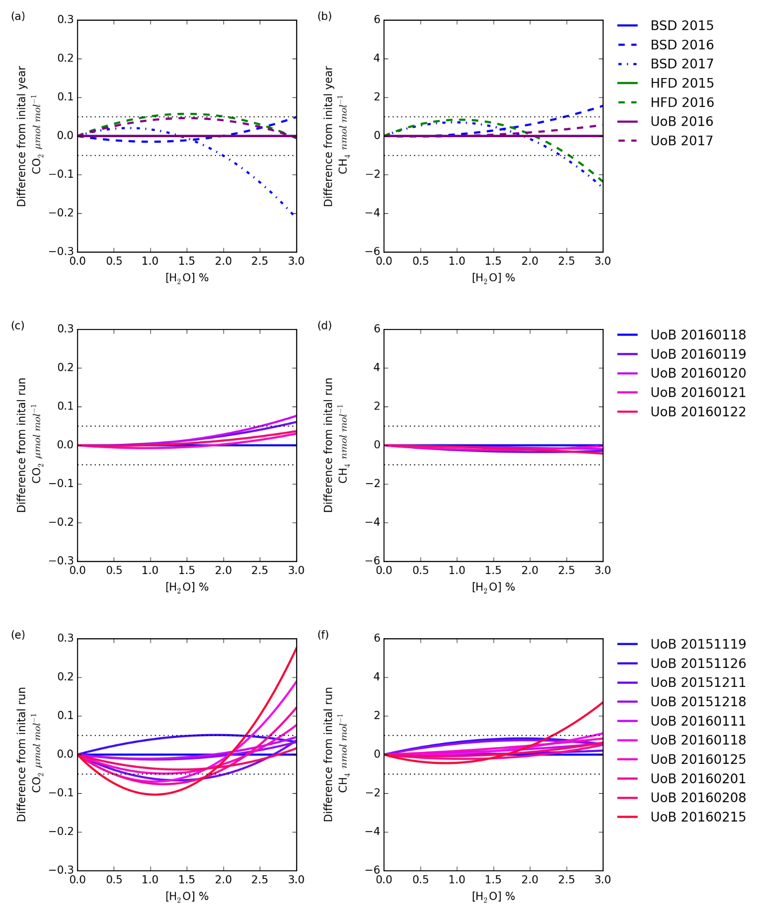
Figure 8The change with water in the difference in CO2 and CH4 dry mole fraction between the first annual mean instrument-specific water correction and subsequent annual corrections (a, b), the first individual water correction and subsequent daily corrections (c, d), and the first individual water correction and subsequent weekly tests (e, f). The daily and weekly tests were conducted using only the UoB instrument while the annual tests were conducted using all three instruments.
The change in the difference between dry mole fractions calculated using the earliest instrument-specific water correction and subsequent water corrections for each instrument with water concentration is shown in Fig. 8a and b. For a typical air sample (1.5 % H2O, 400 µmol mol−1 CO2 and 2000 nmol mol−1 CH4) shifting between the annual water corrections drives CO2 and CH4 changes of < 0.05 µmol mol−1 and < 1 nmol mol−1. However, this difference does change with water content and can increase outside the WMO reproducibility bounds at higher (> 2.5 %) H2O contents. For example, the difference between CO2 dry mole fractions calculated using the Bilsdale 2015 and 2017 H2O correction increases to 0.12 µmol mol−1 at 2.5 % H2O. It is also important to note that these differences will scale with CO2 and CH4 mole fraction. Nevertheless, at the range of ambient water contents observed at BSD and HFD (0.1 % to 2.5 %) these differences remain below the WMO comparability guidelines (WMO, 2018) for CO2 and CH4 mole fractions < 750 µmol mol−1 and < 4000 nmol mol−1 respectively, as observed in BSD and HFD air samples. In light of the temporal variability of the water correction over time at higher water contents for sites with high humidity (> 2 % H2O), using a Nafion® dryer or alternative drying method to obtain a relatively low and stable sample water content would be an advantage.
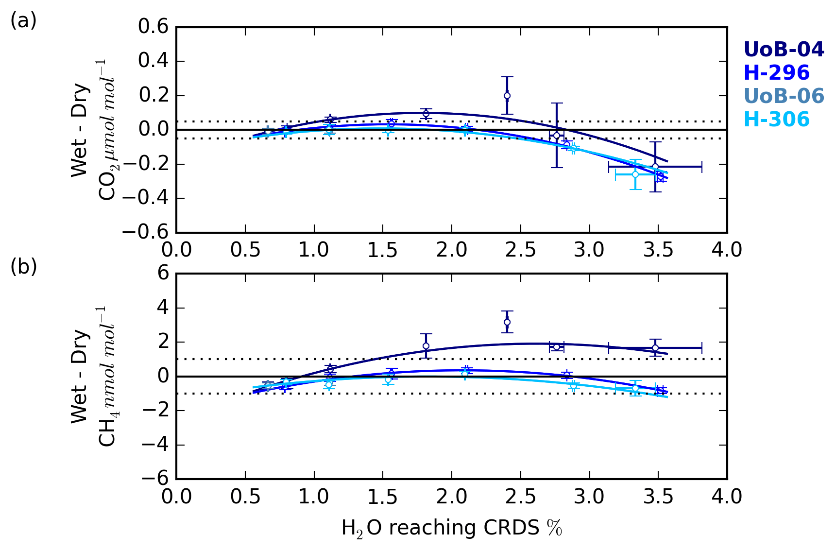
Figure 9The (a) CO2 and (b) CH4 change in the wet–dry sample treatment difference with sample water content for cylinders UoB-04 (515.3 µmol mol−1 CO2 and 2585 nmol mol−1 CH4), H-296 (406.6 µmol mol−1 CO2 and 1947 nmol mol−1 CH4), UoB-06 (384.8 µmol mol−1 CO2 and 1975 nmol mol−1 CH4) and H-306 (372.5 µmol mol−1 CO2 and 1776 nmol mol−1 CH4). Error bars are the larger of either the standard deviation of the mean difference or the uncertainties of the two sample types added together in quadrature.
A comparison of the individual daily and weekly tests, Figs. 8c and d and 10e and f, conducted using the UoB instrument, show the daily tests to be far more similar than the weekly tests. That is, the variability over the 3-month period of the weekly test is much larger than that of the 5 d period of the daily test. However, the variability of the weekly tests is similar to that of the annual tests, Fig. 8a and b, suggesting that, within the bounds of the data typically observed at the BSD and HFD sites, the use of annually derived instrument-specific water corrections is sufficient. This may not be the case at sites with higher levels of humidity and CO2 and CH4 mole fractions where water corrections may need to be determined more frequently, perhaps even weekly. The impracticality of such a frequent testing regime along with the apparent unreliability of the droplet test at H2O > 2.5 % (for example Fig. S8g) mean that an alternative method, possibly partial drying, or a higher level of uncertainty may need to be applied to measurements made at higher water contents.
3.4 Quantifying the CRDS water correction error using the dew point generator
The change in the CRDS water correction with sample H2O content was characterized using the difference between the wet and dry DPG runs. This error typically had a shallow negative parabolic trend for both CO2 and CH4 (Fig. 9) and was similar to the shape seen in the residual of the CRDS water corrections (Figs. S8 and S9) with the error negative at H2O mole fractions near 0.5 %, becoming more positive between 1 % H2O and 2 % H2O before dropping at higher H2O contents.
Although the UoB CRDS was not deployed in the field, we expect the results of the DPG tests to be typical of most Picarro G2401 CO2∕CH4 CRDS instrumentation. The DPG tests show that for ambient and below-ambient mole fraction samples the CH4 error remained within the WMO internal reproducibility guidelines (WMO, 2018) at all water contents examined, that is 0.6 % H2O to 3.5 % H2O, while the CO2 error increased outside the guidelines for H2O > 2.5 %. CO2 errors increased rapidly outside this range, reaching 0.3 µmol mol−1 at 3.5 % H2O. These results are broadly consistent with those of the droplet test residuals.

Figure 10Change in the counter purge in (CPin) and out (CPout) (a) CO2 and (b) CH4 mole fraction with sample water content for ambient (UoB-15) and above-ambient (UoB-16) mole fraction cylinders. Note that the gas stream was cryogenically dried before analysis. Error bars are the larger of either the standard deviation of the mean difference or the uncertainties of the two sample types added together in quadrature. The dotted lines in (a) and (b) are the respective WMO internal reproducibility guidelines.
Unlike the ambient and below-ambient samples, the CRDS water correction error of the above-ambient sample, UoB-04, exceeded the WMO internal reproducibility guidelines for both CO2 and CH4 at most H2O mole fractions. For the H2O range of the BSD and HFD sites the error peaked at 0.1 µmol mol−1 for CO2 near 1.75 % H2O and at 2 nmol mol−1 CH4 near 2.25 % H2O. As discussed earlier in Sect. 3.3, the absolute error in the CRDS water correction will scale with the absolute mole fraction of the sample due to the structure of the correction. The UoB CRDS correction was also optimized using a cylinder of significantly lower mole fraction (397.38 µmol mol−1 CO2 and 1918.73 nmol mol−1 CH4 compared with 515.4 µmol mol−1 and 2579.5 nmol mol−1). This shift in error/residual was also observed in the H2O droplet tests using higher-mole-fraction cylinders, although it appears larger for the DPG tests, most likely due to the higher mole fractions used within these tests (515.4 and 2579.5 compared with 449.55 µmol mol−1 CO2 and 2148 nmol mol−1 CH4 respectively).
The full range of H2O mole fractions observed at the HFD and BSD sites, 0.05 % H2O to 2.5 % H2O, were not examined in these tests, which due to limitations inherent in the experimental set-up were restricted to a H2O range of 0.6 %–3.5 %. However, it is possible to conclude that for observations of ambient and below-ambient CO2 and CH4 mole fractions with H2O > 0.6 % the water-driven error in the CRDS water correction is not likely to be a major source of uncertainty. Even at other DECC sites that are subject to higher humidity, for example the Angus site (Stanley et al., 2018), periods of high (> 2.5 % H2O) water content are rare, < 0.03 % of the data record. In contrast, as elevated CO2 and CH4 mole fractions are regularly observed at both the HFD and BSD sites, the increase in CRDS error with mole fraction is a source of concern and must be quantified as part of a full uncertainty analysis.
3.5 Quantifying Nafion® cross-membrane transport
Nafion® membranes, when combined with a dry counter purge gas stream, can be used to effectively dry air samples. This drying process is driven by the moisture gradient between the wet sample and the dry counter purge. In a similar manner, as long as the membrane is permeable to the gas, a sample-to-counter purge gradient in any other trace gas species will also drive exchange. In an effort to quantify the magnitude of CO2 and CH4 exchange, a series of experiments measuring the composition of the Nafion® counter purge gas were conducted. During these experiments all measurements of the Nafion® counter purge (CPin and CPout) were cryogenically dried to < 0.002 % H2O prior to CRDS analysis. Hence there is a need to use an empirical CRDS water correction and any error associated with the correction was removed and differences between the CPin and CPout samples can be solely attributed to transport across the Nafion® membrane (NX%). The results of these experiments are shown in Fig. 10.
The counter purge experiments conducted with both the ambient (UoB-15) and above-ambient (UoB-16) mole fraction cylinders show identical changes in CO2 and CH4 mole fractions respectively. The wet sample NX% difference is consistently positive for CO2 with the CPout mole fraction an average of 0.021±0.002 µmol mol−1 ( % confidence interval, n > 19) higher than CPin, reflecting a loss from the sample to the counter purge across the Nafion® membrane (Fig. 10a). Although small, this value is an order of magnitude larger than the average standard deviation of the 15 min block means (0.002 µmol mol−1 CO2) making it well within the typical measurement precision. This difference decreases slightly with decreasing sample water content but it is never zero. Even with a dry sample, the CPout–CPin difference (NX%), 0.015±0.003 µmol mol−1 CO2, is still positive. This is in line with previous studies, which have found that, although water substantially increases membrane permeability, even dry membranes are permeable to CO2 (Ma and Skou, 2007; Chiou and Paul, 1988). As earlier studies have found that membranes can take more than a week to fully dry out (Chiou and Paul, 1988), it is also highly likely that the relatively brief length of this study (4 to 5 h) was too short to remove all H2O from the membrane.
Table 5Estimates of the maximum error associated with the measurement of ambient CO2 and CH4 mole fraction samples using the given drying and/or water correction method for the BSD and HFD sites.
The CH4 CPin and CPout mole fraction difference for both dry and wet samples is also slightly positive, 0.03±0.01 and 0.04±0.02 nmol mol−1 CH4 respectively (Fig. 10b). This value is very close to the measurement precision, with the average CH4 standard deviation of the 15 min block means of the order of 0.02 nmol mol−1 CH4.
The ∼0.02 µmol mol−1 loss of CO2 across the Nafion® membrane from the sample stream to the counter purge observed here, although small, is of the order of the WMO internal reproducibility guidelines, 0.05 µmol mol−1 in the Northern Hemisphere and 0.025 µmol mol−1 in the Southern Hemisphere (WMO, 2018), and must be acknowledged. However, the calibration gases are also passed through the Nafion®. These cylinders are very dry, H2O < 0.0001 %, equivalent to the driest conditions studied in the DPG experiments (Fig. 10a) and as such would be expected to show similar CO2 loss across the Nafion® membrane, ∼0.015 µmol mol−1. Hence, as the bias is constant with sample CO2 and H2O mole fractions and as a bias would be present in both the calibration gases (∼0.015 µmol mol−1) and samples (∼0.02 µmol mol−1), the majority of the bias will be calibrated out, with only a very small (≤0.005 µmol mol−1) constant bias, of the order of the instrumental precision, remaining. In contrast, the mean CH4 Nafion® bias, 0.04±0.02 nmol mol−1, is at least an order of magnitude smaller than the WMO internal reproducibility guidelines (WMO, 2018) and is extremely close to the typical measurement precision, suggesting that it is not a bias of concern.
The newly established Bilsdale and Heathfield tall tower measurement stations provide important new data sets of GHG observations. These high-precision continuous in situ measurements show clear long-term increases in baseline CO2, CH4, N2O and SF6 mole fraction and capture the seasonal and diurnal cycles of these key gases. It is expected that these observations, when combined with regional inversion modelling, will significantly improve our ability to quantify UK greenhouse gas emissions – both reducing the uncertainty and improving the spatial and temporal resolution. Future work using these data is focusing on better estimates of UK GHG emissions with a particular emphasis on the UK carbon budget.
The two drying methods implemented at Bilsdale and Heathfield – Nafion® drying with an empirical water correction and an annual empirical water correction without drying – have a number of practical and scientific advantages and disadvantages. The Nafion® drying method, once installed and running correctly can provide reliable drying to between 0.05 % H2O and 0.2 % H2O. While this method requires little ongoing maintenance, if the TOC fails, as has occurred at a number of UoB run tall tower sites, then the replacement of the entire TOC system or removal and repair off site is required. Due to the expense of the TOC instrumentation, having spares available for immediate installation is often not practicable. The sporadic and unpredictable nature of these failures also makes it impossible to incorporate this into routine scheduled site visits. As such, a failure of this nature typically leads to multiple unscheduled trips to the site and periods of poor drying. In contrast, using an annual empirical correction requires a single trip to the site, which can be easily scheduled as part of routine site maintenance. Allowing time for leak checking and at least three replicate droplet tests, such a trip would generally take 2–3 d. As such, for remote or difficult-to-access sites the annual empirical water correction is preferred.
As shown in Table 5, the systematic errors associated with the Nafion® drying method, as applied at these two sites, were small, < 0.01 µmol mol−1 of CO2 and < 0.2 nmol mol−1 of CH4, and did not vary with sample water content. However, care must be taken with the implementation of the method as, for samples with water content > 0.7 %, an additional 0.02 µmol mol−1 of CO2 was lost from the sample across the membrane. Even samples as dry as the calibration gases were affected by this loss, although to a smaller degree (∼0.015 µmol mol−1 for H2O < 0.0001 %) as residual moisture remained in the membrane. However, as in this application of the method the calibration gases are dried in an identical manner to the samples, this loss is mostly calibrated out with only a very small (≤0.005 µmol mol−1) constant residual bias of the order of the instrumental precision. As such, when using a Nafion®-based drying method it is essential that the calibration and standard gases are dried in an identical manner to the samples.
By comparison the annual CRDS empirical water correction has a narrower optimum range with minimal systematic errors only at water contents very near 0 % and between 0.5 % and 2.5 % H2O (Figs. 8, 9, S8 and S9). As such, the choice to use an annual empirical water correction method alone must be strongly influenced by the ambient humidity of the site of interest. Estimates of these systematic errors (Table 5), determined for different water content ranges, were based on the water correction residuals (Fig. S8) and the temporal variability in the annual H2O corrections at each site (Fig. 8a and b). The maximum error associated with the empirical water correction alone ranged between 0.05 and 0.2 µmol mol−1 CO2 and 1 and 3 nmol mol−1 CH4 with the majority of observations at the lower end of the range. It is important to note that these estimates were calculated for the Picarro CRDS and may vary significantly compared to those of other CRDS instrumentation or optical techniques that use alternative cell pressure sensors (Reum et al., 2019).
This weakness in the CRDS water correction also has notable implications for sample drying. Namely, while sample drying may not be an inherent source of bias, the partial drying of the sample puts it within the range of peak error in the CRDS water correction (0.05 % to 0.5 % H2O). This source of error, as demonstrated in the implementation of the Nafion®-based drying system outlined here, can be mitigated by matching the water content of the daily standard to the sample. Again this re-emphasizes the importance of treating the sample, standards and calibration gases in an identical manner.
Considering the relatively narrow humidity range observed at Bilsdale and Heathfield, with no observations > 2.4 % H2O and > 95 % of observations > 0.5 % H2O (> 99 % > 0.35 % H2O) and the relative remoteness of the locations, the decision to remove the Nafion®-based drying systems and rely on the annual empirical water correction appears justified. In contrast, at other more easily accessible or more humid sites the use of a Nafion®-based drying system may be more advantageous.
While these errors are significant relative to the WMO internal reproducibility goals, they are for the majority of observations smaller than the extended WMO measurement compatibility goals (±0.2 µmol mol−1 CO2 and ±5 nmol mol−1 CH4). It is also important to note that they are orders of magnitude smaller than baseline excursions observed at the sites (see Figs. 4 and 5). They are also a factor of 10 smaller than the CH4 model–data mismatch within the UK DECC network as estimated by Ganesan et al. (2015) at ∼20 nmol mol−1. Considering this difference, it is highly unlikely that, without significant improvement in modelled atmospheric transport, the systematic errors reported here would significantly alter estimates of UK-scale GHG fluxes or impede national emissions verification efforts.
Future improvements to the Bilsdale and Heathfield records include the addition of target tanks at the sites. Although the use of target tanks does not directly influence measurement uncertainty, they allow independent long-term monitoring of instrument performance and are a useful tool for assessing measurement uncertainty. The development of a full uncertainty analysis incorporating such target tank measurements along with an assessment of the calibration strategy, instrumental, water correction, and sampling errors and errors induced by the isotopic composition of the calibration gases is also planned. Further work to fully characterize the humidity-dependent error in the water correction of each instrument, like that of Reum et al. (2018), possibly using a piecewise post hoc correction, would also be beneficial in an effort to reduce the estimated error associated with the observations.
The BSD and HFD CO2, CH4 and N2O data are available at http://data.ceda.ac.uk/badc/gauge/data/tower/bilsdale (O'Doherty et al., 2019a) and http://data.ceda.ac.uk/badc/gauge/data/tower/heathfield (O'Doherty et al., 2019b). The CO and SF6 data are not publically available.
The supplement related to this article is available online at: https://doi.org/10.5194/amt-12-4495-2019-supplement.
AS led the paper with contributions from SO, KS, DY, AM, ML, CR and TA. AS designed and performed all drying related experiments and analysed the data. AS, SO, KS, DY, CR and TA shared responsibility for installing, maintaining and managing the data collected at the HFD and BSD sites. AM and ML contributed atmospheric transport modelling outputs and analysis.
The authors declare that they have no conflict of interest.
This article is part of the special issue “Greenhouse gAs Uk and Global Emissions (GAUGE) project (ACP/AMT inter-journal SI)”. It is not associated with a conference.
The National Physical Laboratory (NPL) took responsibility for the Heathfield site on 30 September 2017 through the UK's Department for Business, Energy and Industrial Strategy as part of the National Measurement System programme.
The authors would also like to acknowledge the support of Carole Helfter and Neil Mullinger from the NERC Centre for Ecology and Hydrology (CEH), Edinburgh, Scotland, who helped to maintain and run the Bilsdale site. Lastly the authors would like to thank Joseph Pitt from the University of Manchester for the use of the dew point generator used during a series of preliminary studies.
This study was funded under the NERC Greenhouse Gas Emissions and Feedbacks programme as part of the Greenhouse gAs UK and Global Emissions (GAUGE) area grant number NE/K002449/1NERC. This grant also covered the establishment and early running costs of the stations. Operating costs of the Bilsdale site after 17 September 2016 were funded by the UK Department of Business, Energy and Industrial Strategy (formerly the Department of Energy and Climate Change) through contract TRN1028/06/2015.
This paper was edited by Dominik Brunner and reviewed by two anonymous referees.
Bakwin, P. S., Tans, P. P., Hurst, D. F., and Zhao, C.: Measurements of carbon dioxide on very tall towers: results of the NOAA/CMDL program, Tellus B, 50, 401–415, https://doi.org/10.1034/j.1600-0889.1998.t01-4-00001.x, 1998.
Bouwman, A. F. and Taylor, J. A.: Testing high-resolution nitrous oxide emission estimates against observations using an atmospheric transport model, Global Biogeochem. Cy., 10, 307–318, https://doi.org/10.1029/96gb00191, 1996.
Chen, H., Winderlich, J., Gerbig, C., Hoefer, A., Rella, C. W., Crosson, E. R., Van Pelt, A. D., Steinbach, J., Kolle, O., Beck, V., Daube, B. C., Gottlieb, E. W., Chow, V. Y., Santoni, G. W., and Wofsy, S. C.: High-accuracy continuous airborne measurements of greenhouse gases (CO2 and CH4) using the cavity ring-down spectroscopy (CRDS) technique, Atmos. Meas. Tech., 3, 375–386, https://doi.org/10.5194/amt-3-375-2010, 2010.
Chen, H., Karion, A., Rella, C. W., Winderlich, J., Gerbig, C., Filges, A., Newberger, T., Sweeney, C., and Tans, P. P.: Accurate measurements of carbon monoxide in humid air using the cavity ring-down spectroscopy (CRDS) technique, Atmos. Meas. Tech., 6, 1031–1040, https://doi.org/10.5194/amt-6-1031-2013, 2013.
Chiou, J. S. and Paul, D. R.: Gas permeation in a dry Nafion membrane, Ind. Eng. Chem. Res., 27, 2161–2164, 10.1021/ie00083a034, 1988.
Chris Blandford Associates: North Yorkshire and York Landscape Characterisation Project, London, 2011.
Dlugokencky, E. J.: Trends in Atmospheric Methane, NOAA/ESRL, availabel at: https://www.esrl.noaa.gov/gmd/ccgg/trends_ch4/, last access: 31 July 2015.
Dlugokencky, E. J. and Tans, P.: Trends in Atmospheric Carbon Dioxide, NOAA/ESRL, available at: https://www.esrl.noaa.gov/gmd/ccgg/trends/, last access: 31 July 2015.
Dlugokencky, E. J., Myers, R. C., Lang, P. M., Masarie, K. A., Crotwell, A. M., Thoning, K. W., Hall, B. D., Elkins, J. W., and Steele, L. P.: Conversion of NOAA atmospheric dry air CH4 mole fractions to a gravimetrically prepared standard scale, J. Geophys. Res.-Atmos., 110, D18306, https://doi.org/10.1029/2005JD006035, 2005.
Flores, E., Viallon, J., Moussay, P., Griffith, D. W. T., and Wielgosz, R. I.: Calibration Strategies for FT-IR and Other Isotope Ratio Infrared Spectrometer Instruments for Accurate δ13C and δ18O Measurements of CO2 in Air, Anal. Chem., 89, 3648–3655, https://doi.org/10.1021/acs.analchem.6b05063, 2017.
Foulger, B. E. and Simmonds, P. G.: Drier for field use in the determination of trace atmospheric gases, Anal. Chem., 51, 1089–1090, https://doi.org/10.1021/ac50043a074, 1979.
Fraser, P., Porter, L. W., Baly, S. B., Krummel, P. B., Dunse, B. L., Steele, L. P., Derek, N., Langenfelds, R. L., Levin, I., Oram, D. E., Elkins, J. W., Vollmer, M. K., and Weiss, R. F.: Sulfer hexafluoride at Cape Grim: Long term trends and regional emissions, Baseline Atmospheric (Australia) 2001–2002, 18–23, 2004.
Ganesan, A. L., Manning, A. J., Grant, A., Young, D., Oram, D. E., Sturges, W. T., Moncrieff, J. B., and O'Doherty, S.: Quantifying methane and nitrous oxide emissions from the UK and Ireland using a national-scale monitoring network, Atmos. Chem. Phys., 15, 6393–6406, https://doi.org/10.5194/acp-15-6393-2015, 2015.
Griffith, D. W. T.: Calibration of isotopologue-specific optical trace gas analysers: a practical guide, Atmos. Meas. Tech., 11, 6189–6201, https://doi.org/10.5194/amt-11-6189-2018, 2018.
Hall, B. D., Dutton, G. S., Mondeel, D. J., Nance, J. D., Rigby, M., Butler, J. H., Moore, F. L., Hurst, D. F., and Elkins, J. W.: Improving measurements of SF6 for the study of atmospheric transport and emissions, Atmos. Meas. Tech., 4, 2441–2451, https://doi.org/10.5194/amt-4-2441-2011, 2011.
Hammer, S., Glatzel-Mattheier, H., Muller, L., Sabasch, M., Schmidt, M., Schmitt, S., Schonherr, C., Vogel, F., Worthy, D., and Levin, I.: A gas chromatographic system for high-precision quasi-continuous atmospheric measurements of CO2, CH4, N2O, SF6, CO and H2, available at: https://www.researchgate.net/publication/255704060_A_gas (last access: 26 October 2018), 2008.
Hunter, J. D.: Matplotlib: A 2D Graphics Environment, Comput. Sci. Eng., 9, 90–95, https://doi.org/10.1109/MCSE.2007.55, 2007.
IPCC: Summary for Policymakers, in: Climate Change 2013: The Physical Science Basis, Contribution of Working Group I to the Fifth Assessment Report of the Intergovernmental Panel on Climate Change, edited by: Stocker, T. F., Qin, D., Plattner, G.-K., Tignor, M., Allen, S. K., Boschung, J., Nauels, A., Xia, Y., Bex, V., and Midgley, P. M., Cambridge University Press, Cambridge, UK and New York, NY, USA, 1–30, 2013.
Jones, E., Oliphant, E., Peterson, P., et al.: SciPy: Open Source Scientific Tools for Python, 2001-, available at: http://www.scipy.org/, last access: 20 August 2019.
Ma, S. and Skou, E.: CO2 permeability in Nafion® EW1100 at elevated temperature, Solid State Ionics, 178, 615–0619, https://doi.org/10.1016/j.ssi.2007.01.030, 2007.
Manning, A. J., O'Doherty, S., Jones, A. R., Simmonds, P. G., and Derwent, R. G.: Estimating UK methane and nitrous oxide emissions from 1990 to 2007 using an inversion modeling approach, J. Geophys. Res.-Atmospheres, 116, D02305, https://doi.org/10.1029/2010JD014763, 2011.
Nara, H., Tanimoto, H., Tohjima, Y., Mukai, H., Nojiri, Y., Katsumata, K., and Rella, C. W.: Effect of air composition (N2, O2, Ar, and H2O) on CO2 and CH4 measurement by wavelength-scanned cavity ring-down spectroscopy: calibration and measurement strategy, Atmos. Meas. Tech., 5, 2689–2701, https://doi.org/10.5194/amt-5-2689-2012, 2012.
Naudy, S., Collette, F., Thominette, F., Gebel, G., and Espuche, E.: Influence of hygrothermal aging on the gas and water transport properties of Nafion® membranes, J. Membrane Sci., 451, 293–304, https://doi.org/10.1016/j.memsci.2013.10.013, 2014.
Nevison, C. D., Dlugokencky, E., Dutton, G., Elkins, J. W., Fraser, P., Hall, B., Krummel, P. B., Langenfelds, R. L., O'Doherty, S., Prinn, R. G., Steele, L. P., and Weiss, R. F.: Exploring causes of interannual variability in the seasonal cycles of tropospheric nitrous oxide, Atmos. Chem. Phys., 11, 3713–3730, https://doi.org/10.5194/acp-11-3713-2011, 2011.
North York Moors National Park Authority: North York Moors National Park Management Plan: A wider view, Helmsley, 2012.
Novelli, P. C., Elkins, J. W., and Steele, L. P.: The development and evaluation of a gravimetric reference scale for measurements of atmospheric carbon monoxide, J. Geophys. Res.-Atmos., 96, 13109–13121, https://doi.org/10.1029/91JD01108, 1991.
O'Doherty, S., Say, D., and Stanley, K.: Deriving Emissions related to Climate Change Network: N20, SF6, CO, H2 and other trace gas species measurements from Bilsdale Tall Tower, North York Moors National Park, Centre for Environmental Data Analysis, available at: http://data.ceda.ac.uk/badc/gauge/data/tower/bilsdale/, last access: 20 August 2019a.
O'Doherty, S., Say, D., and Stanley, K.: Deriving Emissions related to Climate Change Network: N20, SF6, CO, H2 and other trace gas species measurements from Heathfield Tall Tower, North York Moors National Park, Centre for Environmental Data Analysis, available at: http://data.ceda.ac.uk/badc/gauge/data/tower/heathfield/, last access: 20 August 2019b.
Prinn, R., Cunnold, D., Rasmussen, R., Simmonds, P., Alyea, F., Crawford, A., Fraser, P., and Rosen, R.: Atmospheric emissions and trends of nitrous oxide deduced from 10 years of ALE–GAGE data, J. Geophys. Res.-Atmos., 95, 18369–18385, https://doi.org/10.1029/JD095iD11p18369, 1990.
Rella, C.: Accurate Greenhouse Gas Measurements in Humid Gas Streams Using the Picarro G1301 Carbon Dioxide/Methane/Water Vapor Gas Analyzer, 2010.
Rella, C. W., Chen, H., Andrews, A. E., Filges, A., Gerbig, C., Hatakka, J., Karion, A., Miles, N. L., Richardson, S. J., Steinbacher, M., Sweeney, C., Wastine, B., and Zellweger, C.: High accuracy measurements of dry mole fractions of carbon dioxide and methane in humid air, Atmos. Meas. Tech., 6, 837–860, https://doi.org/10.5194/amt-6-837-2013, 2013.
Reum, F., Gerbig, C., Lavric, J. V., Rella, C. W., and Göckede, M.: Correcting atmospheric CO2 and CH4 mole fractions obtained with Picarro analyzers for sensitivity of cavity pressure to water vapor, Atmos. Meas. Tech., 12, 1013–1027, https://doi.org/10.5194/amt-12-1013-2019, 2019.
Satar, E., Berhanu, T. A., Brunner, D., Henne, S., and Leuenberger, M.: Continuous measurements (2012–2014) at Beromünster tall tower station in Switzerland, Biogeosciences, 13, 2623–2635, https://doi.org/10.5194/bg-13-2623-2016, 2016.
Schibig, M. F., Steinbacher, M., Buchmann, B., van der Laan-Luijkx, I. T., van der Laan, S., Ranjan, S., and Leuenberger, M. C.: Comparison of continuous in situ CO2 observations at Jungfraujoch using two different measurement techniques, Atmos. Meas. Tech., 8, 57–68, https://doi.org/10.5194/amt-8-57-2015, 2015.
Stanley, K. M., Grant, A., O'Doherty, S., Young, D., Manning, A. J., Stavert, A. R., Spain, T. G., Salameh, P. K., Harth, C. M., Simmonds, P. G., Sturges, W. T., Oram, D. E., and Derwent, R. G.: Greenhouse gas measurements from a UK network of tall towers: technical description and first results, Atmos. Meas. Tech., 11, 1437–1458, https://doi.org/10.5194/amt-11-1437-2018, 2018.
Tans, P. P., Crotwell, A. M., and Thoning, K. W.: Abundances of isotopologues and calibration of CO2 greenhouse gas measurements, Atmos. Meas. Tech., 10, 2669–2685, https://doi.org/10.5194/amt-10-2669-2017, 2017.
Topp, E. and Pattey, E.: Soils as sources and sinks for atmospheric methane, Can. J. Soil Sci., 77, 167–177, https://doi.org/10.4141/S96-107, 1997.
Turnbull, J. C., Sweeney, C., Karion, A., Newberger, T., Lehman, S. J., Tans, P. P., Davis, K. J., Lauvaux, T., Miles, N. L., Richardson, S. J., Cambaliza, M. O., Shepson, P. B., Gurney, K., Patarasuk, R., and Razlivanov, I.: Toward quantification and source sector identification of fossil fuel CO2 emissions from an urban area: Results from the INFLUX experiment, J. Geophys. Res.-Atmos., 120, 292–312, https://doi.org/10.1002/2014JD022555, 2015.
van der Laan, S., Neubert, R. E. M., and Meijer, H. A. J.: A single gas chromatograph for accurate atmospheric mixing ratio measurements of CO2, CH4, N2O, SF6 and CO, Atmos. Meas. Tech., 2, 549–559, https://doi.org/10.5194/amt-2-549-2009, 2009.
van der Walt, S., Colbert, S. C., and Varoquaux, G.: The NumPy Array: A Structure for Efficient Numerical Computation, Comput. Sci. Eng., 13, 22–30, https://doi.org/10.1109/MCSE.2011.37, 2011.
van Rossum, G.: Python tutorial, Technical Report CS-R9526, Centrum voor Wiskunde en Informatica (CWI), Amsterdam, 1995.
Welp, L. R., Keeling, R. F., Weiss, R. F., Paplawsky, W., and Heckman, S.: Design and performance of a Nafion dryer for continuous operation atCO2 and CH4 air monitoring sites, Atmos. Meas. Tech., 6, 1217–1226, https://doi.org/10.5194/amt-6-1217-2013, 2013.
Winderlich, J., Chen, H., Gerbig, C., Seifert, T., Kolle, O., Lavrič, J. V., Kaiser, C., Höfer, A., and Heimann, M.: Continuous low-maintenance measurements at the Zotino Tall Tower Observatory (ZOTTO) in Central Siberia, Atmos. Meas. Tech., 3, 1113–1128, https://doi.org/10.5194/amt-3-1113-2010, 2010.
WMO: 19th WMO/IAEA Meeting on Carbon Dioxide, Other Greenhouse Gases and Related Measurement Techniques (GGMT-2017) Geneva, Switzerland, 2018.
Young, D.: Development of a Pre-Concentration System for the Determination of Atmospheric Oxygenated Volatile Organic Compounds, Doctor of Philosphy, School of Chemistry, Faculty of Science, University of Bristol, Bristol, 2007.
Yver Kwok, C., Laurent, O., Guemri, A., Philippon, C., Wastine, B., Rella, C. W., Vuillemin, C., Truong, F., Delmotte, M., Kazan, V., Darding, M., Lebègue, B., Kaiser, C., Xueref-Rémy, I., and Ramonet, M.: Comprehensive laboratory and field testing of cavity ring-down spectroscopy analyzers measuring H2O, CO2, CH4 and CO, Atmos. Meas. Tech., 8, 3867–3892, https://doi.org/10.5194/amt-8-3867-2015, 2015.
Zhao, C. L. and Tans, P. P.: Estimating uncertainty of the WMO mole fraction scale for carbon dioxide in air, J. Geophys. Res.-Atmos., 111, D08s09 https://doi.org/10.1029/2005jd006003, 2006.