Methodology for high-quality mobile measurement with focus on black carbon and particle mass concentrations

Measurements of air pollutants such as black carbon (BC) and particle mass concentration in general, using mobile platforms equipped with high-time-resolution instruments, have gained popularity over the last decade due to their wide range of applicability. Assuring the quality of mobile measurement, data have become more essential, particularly when the personal exposure to pollutants is related to their spatial distribution. In the following, we suggest a methodology to achieve data from mobile measurements of equivalent black carbon (eBC) and PM_2.5 mass concentrations with high data quality. Besides frequent routine quality assurance measures of the instruments, the methodology includes the following steps: (a) measures to ensure the quality of mobile instruments through repeated collocated measurements using identical instrumentation, (b) inclusion of a fixed station along the route containing quality-assured reference instruments, and (c) sufficiently long and frequent intercomparisons between the mobile and reference instruments to correct the particle number and mass size distributions obtained from mobile measurements. The application of the methodology can provide the following results. First, collocated mobile measurements with sets of identical instruments allow identification of undetected malfunctions of the instruments. Second, frequent intercomparisons against the reference instruments will ensure the quality of the mobile measurement data of the eBC mass concentration. Third, the intercomparison data between the mobile optical particle size spectrometer (OPSS) and a reference mobility particle size spectrometer (MPSS) allow for the adjustment of the OPSS particle number size distribution using physically meaningful corrections. Matching the OPSS and MPSS volume particle size distributions is crucial for the determination of PM_2.5 mass concentration. Using size-resolved complex refractive indices and time-resolved fine-mode volume correction factors of the fine-particle range, the calculated PM_2.5 from the OPSS was within 5 % of the reference instruments (MPSS+APSS). However, due to the nonsphericity and an unknown imaginary part of the complex refractive index of supermicrometer particles, a conversion to a volume equivalent diameter yields high uncertainties of the particle mass concentration greater than PM_2.5. The proposed methodology addresses issues regarding the quality of mobile measurements, especially for health impact studies, validation of modeled spatial distribution, and development of air pollution mitigation strategies.

1 Introduction

Mobile measurements of particulate air pollutants, which are often performed with portable instruments on mobile platforms, have been a trend in air quality monitoring for the past decade. The fast measurements, ease of use, and relatively low costs have appealed to air quality scientists for their applications on air quality mapping (Ghassoun et al., 2015; Ruths et al., 2014), exposure studies (Peters et al., 2014; Birmili et al., 2013; Patton et al., 2014; Williams and Knibbs, 2016), and emission factor estimates (Ježek et al., 2015; Karjalainen et al., 2014). In particular, this has been widely used to measure air pollutants which have high spatial and temporal variabilities such as black carbon (or equivalent black carbon – eBC – when measured optically according to Petzold et al., 2013) or the particulate matter (PM) mass concentration (Peters et al., 2014; Rakowska et al., 2014) and which have significant impacts on both climate and health issues. However, mobile measurements encounter many challenges. Firstly, due to the mobile, and therefore unstable, nature of the measurements, the small and portable instruments might be sensitive to vibrations and sudden changes in ambient conditions, leading often to false data (Cai et al., 2013; Apte et al., 2011). Secondly, to achieve a concentration representative of the chosen route, measurements have to be done along fixed routes and with a high number of repeated runs, requiring considerable time and effort. Thirdly, optical particle size spectrometers (OPSSs), which are often preferred for particle mass concentration measurements, have a limited size range and depend highly on the aerosol particle optical properties. The OPSS is a practical choice for measuring size-resolved PM mass concentration for mobile measurements because of its portability, relatively low cost, and near-real-time measurements. However, the OPSS does not measure the volume equivalent particle diameter. The OPSS measures the optical particle diameter based on scattered light and related to the refractive index of the calibration aerosol. The sizing of the OPSS relies then on the calibration response curve that is based on well-defined particles such as certified polystyrene latex (PSL) spheres with known refractive index. However, real word scenarios involve particles with varying optical properties which can result in erroneous sizing for the OPSS. Studies (Chien et al., 2016; Rosenberg et al., 2012; Binnig et al., 2007) have suggested ways to improve OPSS data through different calibration and postprocessing techniques, mainly to relate optical diameter to aerodynamic diameter, with the latter being the more relevant for health studies. However, to calculate mass concentrations of PM, especially for PM_2.5, the optical diameter has to be related to the volume equivalent diameter and not aerodynamic.

There is a wide variety of portable instruments in the market such as for eBC and PM mass concentration. However, the performance of these instruments (especially the commercialized, low-cost sensors) and the differences of the mobile measurement methods employed are still questionable. This may often lead to unreliable, misleading, and noncomparable data, especially for health impact studies, validation of modeled spatial distribution, and development of air pollution mitigation strategies (Castell et al., 2017).

In the last 5 years, several studies have explored different approaches, both for the measurement procedure and data processing to increase the quality and reliability of mobile measurement data. Birmili et al. (2013) emphasized the importance of regular intercomparisons of the portable devices against reference instruments prior to and during mobile measurement campaigns. Cai et al. (2013) suggested the use of a diffusion dryer before an absorption photometer for eBC measurements to optimize the instrument for personal exposure characterization. More recently, Yu et al. (2016) suggested to measure simultaneously on parallel streets to disentangle the spatial from the temporal variability. Concerning the handling of mobile measurement data, Van den Bossche et al. (2015) and Van Poppel et al. (2013) suggested guidelines for pollutants measured with a bicycle. For example, they suggested exploring different statistics in aggregating data spatially to eliminate the impacts of single events and perform background normalization to determine the influence of local emissions. However, to our knowledge, there are no comprehensive guidelines for mobile measurements of both eBC and PM mass concentrations with a focus on pedestrian exposure.

The main goal of this article is to propose a methodology for mobile measurements and data processing, which would provide reliable and quality-assured data of spatially resolved eBC and PM mass concentrations for scientific purposes. Specifically, we propose measurements and postprocessing techniques based on meaningful physical assumptions by addressing the limitations of an OPSS. Measurements from an intensive campaign in Rome, Italy, were used to demonstrate the proposed methodology.

2 Methodology for quality-assured mobile measurements

This methodology was developed around existing, frequently used, portable instruments as well as highly characterized reference instruments for eBC and PM mass concentration measurements (see Table 1). It is divided into three parts: (1) methods to ensure quality of mobile instruments and measurements, (2) methods to ensure the quality of the reference instruments, and (3) mobile measurement strategy and data correction to derive PM mass concentrations from OPSS particle number size distribution (PNSD) measurements.

Table 1 Description of portable and reference instruments. Additional details are provided in Appendix A.

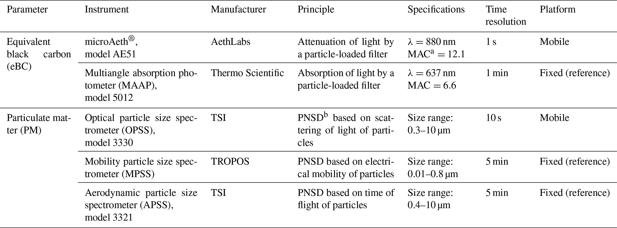
^a MAC: mass absorption coefficient (m² g⁻¹). ^b PNSD: particle number size distribution.

The following methodology (Fig. 1) is proposed to obtain high-quality data from mobile measurements. Note that the items with an asterisk correspond to instrument-specific methodology based on target air pollutant.

1. Mobile instrumentation and measurements.

   • Instrument checks and calibration before and after the campaign.

   • Designing of a strategic fixed mobile measurement route.

   • Assuring the quality of mobile measurement data through prerun protocols or routine.

   • Application of identical mobile instrumentation through collocated mobile measurements.

   • Multiple mobile measurements to achieve representative spatial distribution of concentration.

2. Fixed station measurements with reference instruments.

   • Instrument calibration and verification before and after the campaign.

   • Selection of a background site which is part of the fixed mobile measurement route.

   • Regular checks and calibration of instruments during campaign (once per week).

   • Merging of mobility particle size spectrometer (MPSS) and aerodynamic particle size spectrometer (APSS) size distribution*.

3. Sufficiently long and frequent intercomparison periods between the fixed and mobile instruments*.

   • Intercomparison of the eBC mass concentration from the mobile platform against the reference absorption photometer*.

   • Adjustment of the OPSS PNSD to the one of the reference MPSS according to aerosol-type-dependent complex refractive index*.

   • Determination of time-dependent fine-mode volume correction factor*.

   • Calculation of PM_2.5 mass concentration*.

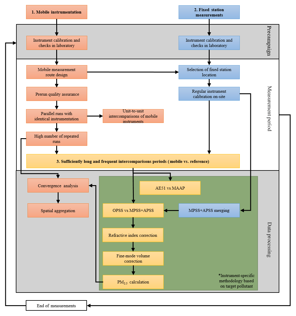
Figure 1 Methodology for highly quality assured mobile measurements. The task box colors distinguish methods 1, 2, and 3 while the color of the background separates the period of the application of each method. The green box represents the items in the methodology that are instrument-specific. For the purposes of this article, the items within the green box are tailored for eBC and PM measurements from AE51 and OPSS, respectively.

3 Exemplary measurements

To demonstrate the proposed methodology, we used the dataset from a mobile measurement experiment that was part of an intensive campaign called Carbonaceous Aerosols in Rome and Environs (CARE) in the downtown area of Rome, Italy, in February of 2017. The scientific aim of CARE was to characterize the carbonaceous aerosol in the Mediterranean urban background area of Rome. An overview of this campaign and the first results are presented by Costabile et al. (2017).

3.1 Mobile instrumentation and measurements

Mobile measurements or “runs” of eBC and PM were carried out using the following instruments which are portable and have high time resolution: an absorption photometer (microAeth^®, model AE51, AethLabs, San Francisco, CA, USA) and the optical particle size spectrometer (OPSS, model 3330, TSI Inc., Shoreview, MN, USA), respectively. Specifications of these instruments are in Table 1. These instruments were placed inside a mobile measurement platform called an aerosol backpack (Fig. A1) together with a GPS and a microcomputer for data acquisition. A detailed description of the aerosol backpack is in Appendix A.

3.1.1 Calibration of instruments before and after the campaign

Prior to a measurement campaign, the mobile instruments must undergo a series of quality checks in the laboratory such as leak check, flow check and flow calibrations, unit-to-unit intercomparison, and most importantly intercomparisons with reference instruments. These should be done to ensure that the mobile instruments are operating correctly and provide high-quality data before deployment. In this case, the AE51 units must be compared against a well characterized and calibrated optical absorption photometer such as a multiangle absorption photometer (MAAP, model 2012, Thermo, Inc., Waltham, MA USA), provided that both are connected to the same inlet with ambient air to test the performance of the AE51 in real-world scenarios. The OPSS, on the other hand, must be subjected to a size calibration using a mixture of polystyrene latex (PSL) particles of known sizes. The same procedure should be done after a measurement campaign.

3.1.2 Designing of a strategic fixed mobile measurement route

The fixed mobile measurement route must be strategically designed to address the study-specific science question(s). This includes careful consideration of the street topography, the length of the route, and the time it takes to complete. The route should include different microenvironments to capture the spatial variability of the pollutant concentration. For this study, the fixed route (Fig. 2) was approximately 9 km long and took 2.5 h to complete. This route covered different microenvironments to simulate varying exposure scenarios: a park area, roadside, intersections, street canyons, street cross sections, residential and commercial areas, and a gated garden.

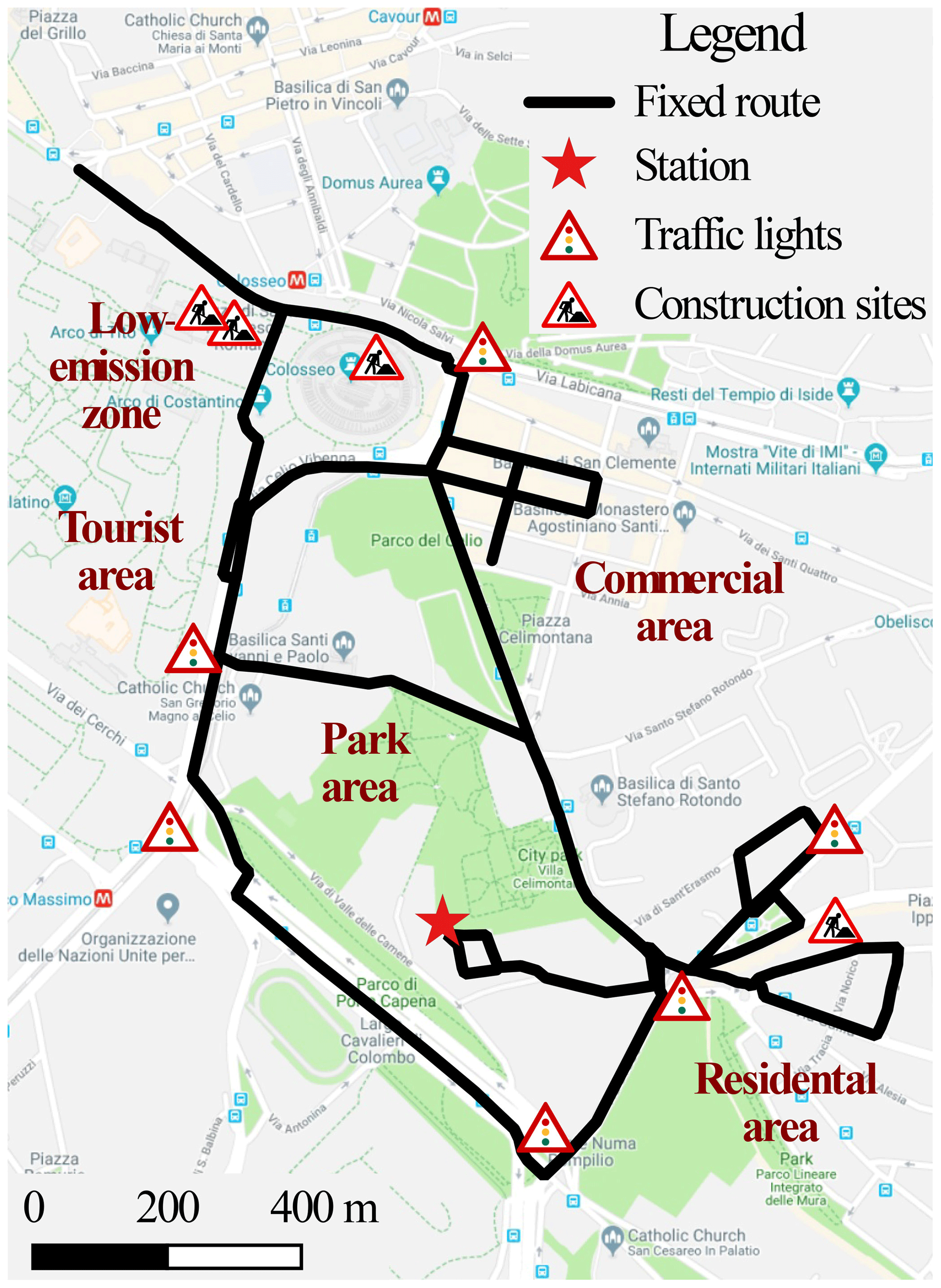
Figure 2 Illustration of the fixed mobile measurement route with labels of the different microenvironments. Map data © Google Maps 2015.

3.1.3 Assuring the quality of mobile measurement data through prerun protocols or routine

Each mobile measurement period should include a prerun routine: (1) checking for leaks within the systems by placing a total filter on the inlet, (2) giving ample time for the instruments to warm up (depending on the instruments used), (3) measuring the total flow of the system, and (4) synchronizing the time of the two microcomputers or data loggers of each backpack. Additionally, if the prerun routine is done indoors, then once stepping outside, the GPS should be given enough time to find satellites to get accurate location data before starting the run. Other instrument-specific routines should also be included. For instance, in this study, the filter of the AE51 has to be replaced before each run to avoid filter saturations.

3.1.4 Application of identical mobile instrumentation through collocated mobile measurements

Deploying a single aerosol backpack may be more practical; however, there is a risk of completing a sampling period without knowing if the data are valid, especially in the absence of real-time data viewing. This is highly likely for portable instruments which are sensitive to vibrations, sudden movements, and changes in their immediate environment. Here we demonstrate the advantage of performing collocated measurements with two aerosol backpacks containing identical instrumentation carried by two “runners”.

Having two identical aerosol backpacks opens several possibilities for mobile measurements. One example is to determine the spatial variability of pollutants by deploying each aerosol backpack in parallel streets at the same time (Yu et al., 2016). This way, the spatial aspect can be separated from the temporal. One can also perform runs along the same route but 30 min apart or so. This would result in a high number of data points leading to increased representativeness of the overall spatial average. These two examples are best applied when data can be viewed and checked in real time so the quality is not compromised. Another way is to target quality assurance by doing side-by-side parallel runs or collocated measurements as done here. This allows for a constant quality check of the mobile instruments along the whole route, since live visualization of data is not available, particularly in locations without reference instruments to compare with. During this campaign, mobile measurement data can only be checked after the run, and, consequently, errors can only be noticed during the postprocessing of the data. For example, during the early stages of the campaign, analysis of the collocated measurements revealed that one AE51 was underestimating eBC mass concentrations by 50 % due to weakening of the pump causing the flow to decrease. This was not flagged by the instrument, but because another AE51 was in operation, the error was identified and corrected immediately. Similarly, towards the end of the campaign, due to unidentified reasons, the sheath flow of one of the OPSS started to increase, which resulted in an underestimation of the particle number concentration (PNC) across all size bins (19 %–80 %). This was not flagged by the instrument and was only noticed when compared against the other OPSS. By comparing the data gathered from the two aerosol backpacks postrun, errors in the data were easily noticed, investigated, and corrected, especially errors that were not flagged by the instruments (i.e., sheath flow drift, time shift, etc.).

To demonstrate the advantage of this approach, an example of a time series from one run is shown in Fig. 3. The topmost panel shows the time series of eBC mass concentrations from the two AE51s in 10 s resolution (median). While the last two panels show the time series of PNC at 0.417 and 2.406 µm, respectively, measured by the two OPSSs. The scatter plots on the right of each time series show the correlation between the two corresponding instruments. The collocated measurements show the performance of the mobile instruments throughout the whole route, which are in good agreement with each other. The peaks in the data represent the parts of the route which are closer to sources such as street sides and intersections. The correlation analyses show that the unit-to-unit variability of the two AE51s was within 10 % and within 5 % for the two channels shown here for the OPSS units. The small discrepancies between the mobile instruments are attributed to instrument uncertainty. Large differences, on the other hand, were investigated further to determine if they are related to sources or technical malfunctions. For example, in one of the runs, the pump of AE51 (2) was not working properly, making the sample flow 50 % lower than desired. A comparison with AE51 (1) showed that the eBC mass concentration measured by AE51 (2) was underestimated. This was also verified through intercomparison against the MAAP. Hence, the eBC measurements from AE51 (2) during this run were removed from the dataset. Similar cases were filtered out during the data selection process.

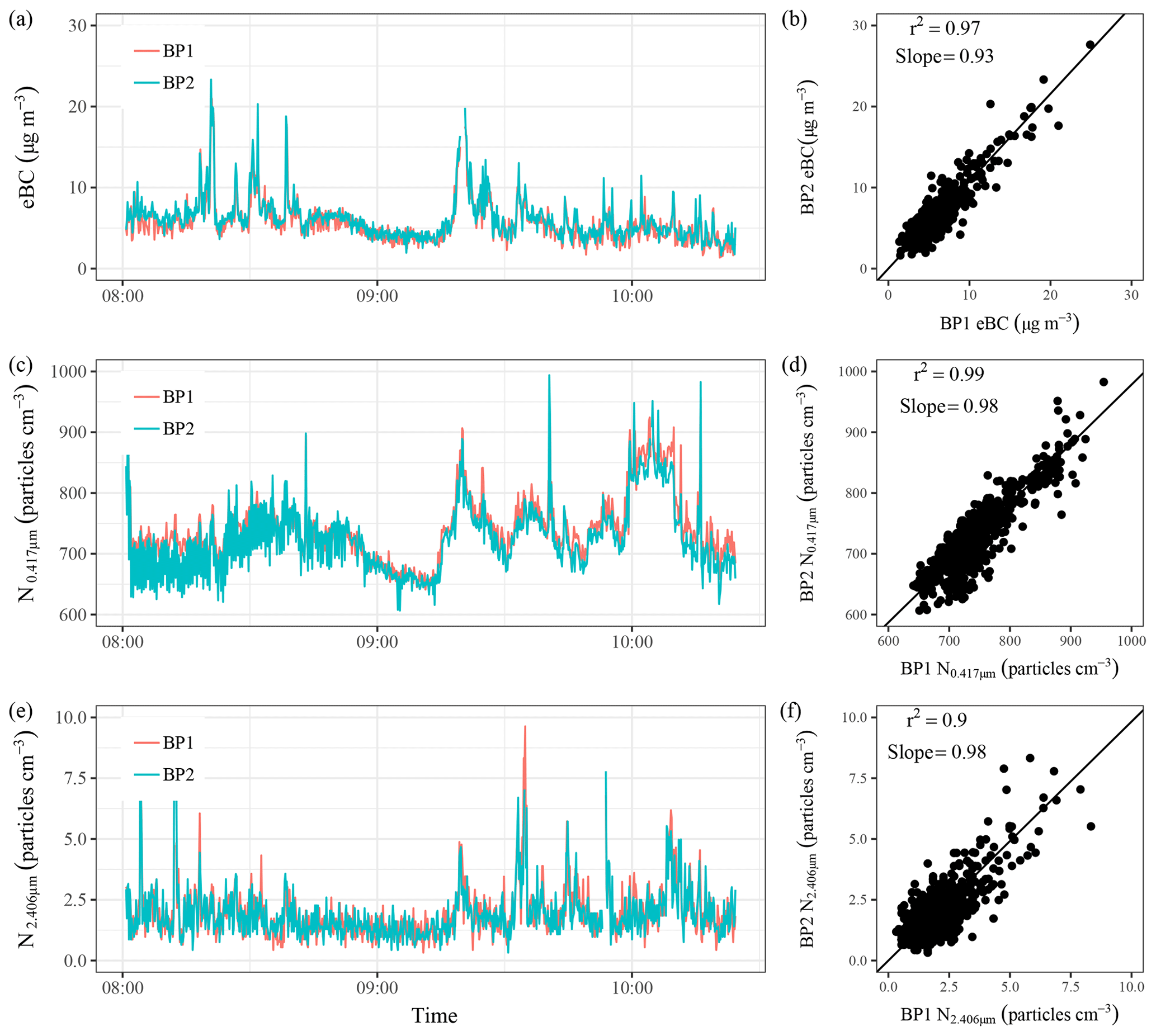
Figure 3 The 10 s resolution time series of eBC (a) and PNC from two channels (c, e) of the OPSS from one parallel run. The panels on the right show the correlation between the AE51s (b) and OPSSs (d, f) using standard major axis regression to account for the error on both axes.

3.1.5 Multiple mobile measurements to achieve representative spatial distribution of concentration

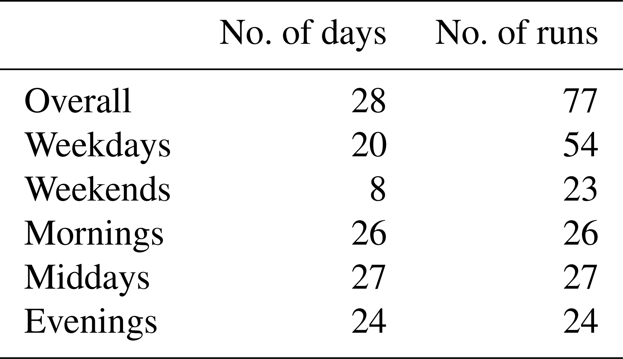
Pollutants such as BC and PM_2.5 can be highly variable in space and time, especially at ground level in urban areas. Determining the spatial distribution of these pollutants that is representative of the study area would require a high number of repeated measurements over different periods to minimize the impacts of single events such as a passing of a heavy-duty vehicle or the presence of a temporary construction area. Furthermore, frequent runs will also average out the influence of meteorology such as dynamics of the boundary layer and different wind conditions. Here, we demonstrate the advantage of performing a high number of runs along a fixed route. Runs were done three times a day (morning rush hour, midday, and evening rush hour), on weekdays and weekends, for 1 whole month. This resulted in a total of 77 runs, distributed across conditions as shown in Table 2.

Table 2 Summary of mobile measurement runs during the CARE campaign.

Minimizing the impacts of single events can also be achieved by choosing an appropriate averaging method for the data collected within a run. Van den Bossche et al. (2015) have investigated the results of using different averaging methods and concluded that minimizing the impacts of single events is best achieved by using the trimmed mean. Others (Peters et al., 2013; Brantley et al., 2014; Alas et al., 2018) have argued that the use of the median is more robust to bias due to single events. The selection of an averaging method depends on the scientific question for a particular study. Here, the nonoverlapping interval 10 s median was used in order to maintain a high spatial resolution.

Convergence analysis

As previously stated, spatial data are highly variable because of many factors, and a single or a few runs will not provide a representative estimate of the spatial distribution. Data experiments to determine the number of runs necessary to achieve a representative estimate of pollutant concentration based on mobile measurements have been introduced by Peters et al. (2013), Van Poppel et al. (2013), and Van den Bossche et al. (2015). The idea is to take the pollutant concentrations measured per run along a specific part of the route and then take the cumulative (increasing number of runs) average (or median) of those concentrations. This procedure is done with a high number of iterations to achieve a high number of possible combinations of the runs. Convergence is achieved when the iterations has stabilized to an asymptotic behavior towards the desired metric (e.g., median concentration from that location from all runs). The number of runs when the iterations are within the specified threshold of deviation from the selected metric (criteria for convergence) then tells how many runs are needed to achieve the representative concentration. The criteria for convergence depend on the science question and goals to be achieved. Previous experiments have used convergence criteria based on required accuracy of PM_2.5 mass concentrations obtained from air quality monitoring stations (25 %) and indicative measurements (50 %), and the latter was used in this study for demonstration. Figure 4 shows the results of the convergence analysis performed on a street canyon and a park area as examples. For the park, since there are no direct sources (it is inaccessible to vehicles) the data converged faster at 56 runs, while in the street canyon, which has higher variability because of traffic emissions, convergence was achieved at 67 runs. This shows that for routes containing regions with higher concentration variability, mobile measurements must be conducted with a higher number of repetitions. It must be emphasized, however, that one must consider a threshold that accounts for the natural variability of the pollutant concentration.

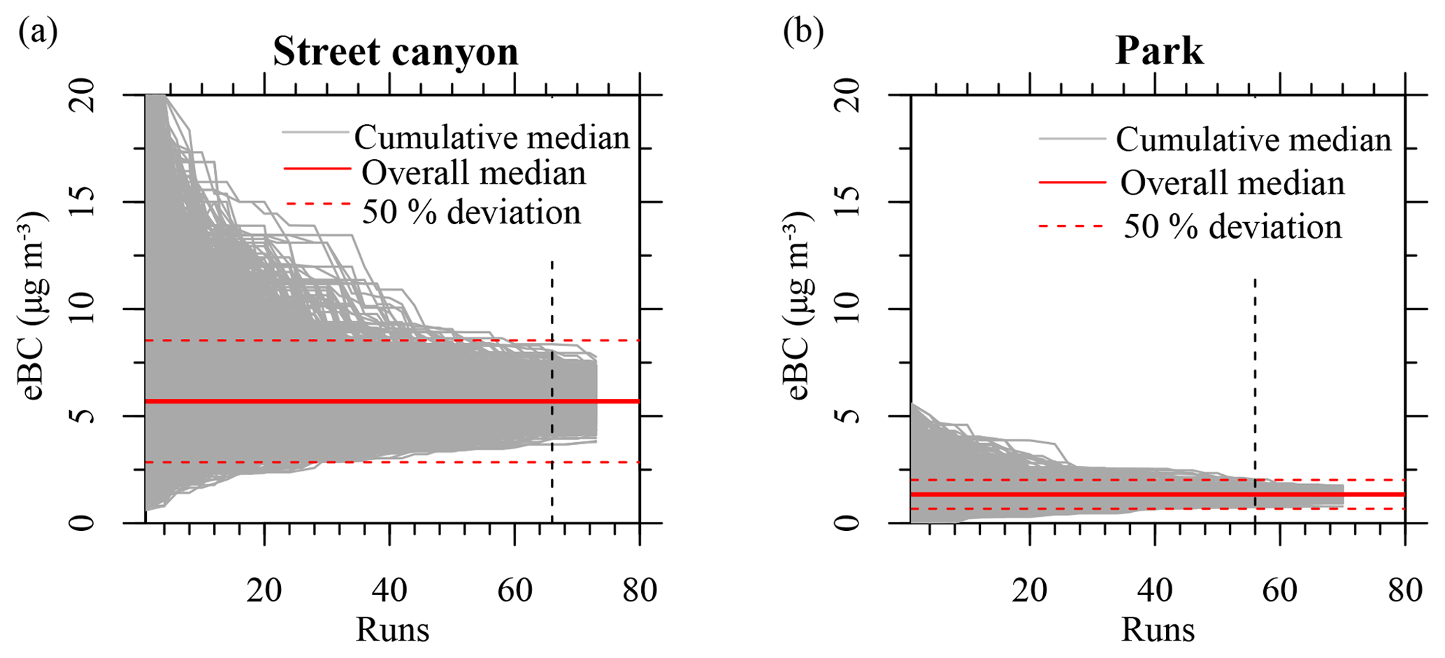
Figure 4 Convergence analysis performed on data points in the (a) street canyon and (b) park area. The vertical dashed line marks the number of runs where convergence was reached.

Spatial averaging

The data points resulting from mobile measurements do not exactly fall on the same point in space and time. The time resolution of the instruments and the uncertainty of the GPS contribute to this. Figure 5 shows the cloud of data points (purple dots) acquired from all runs. Therefore, to obtain the overall spatial distribution, the data points have to be spatially aggregated. Prior to spatial aggregation, the data cloud has to be cleaned by removing data points that are not part of the route (e.g., detours, inaccurate GPS points). The spatial aggregation method used in this study was that of Alas et al. (2018). Briefly, the predetermined route was created with equidistant points (0.0002^∘, or ∼23 m; green dots in Fig. 5a). The distance between the two points depends on the desired spatial resolution. The data points are projected on a map as a data cloud. These points, particularly the ones that are not on the street due to GPS uncertainty, are snapped back onto the nearest street using a point-snapping algorithm. The predetermined route was used as center points for spatial aggregation. The median of all the data points falling within a user-defined radius around each center point (in this study 0.0005^∘, or ∼56 m) is calculated, resulting in a moving circular median. Figure 5b shows the result of the spatial aggregation, with the colors indicating the pollutant concentration – in this case, the eBC mass concentration.

Figure 5 Illustration of the spatial averaging performed on the mobile measurement data (a) showing all the data points in purple dots and the center points for averaging in green and (b) with the spatial average of eBC mass concentrations for the entire campaign. Map data © Google Maps 2015.

3.2 Fixed station measurements

Table 1 describes the reference instruments, and brief descriptions of the fixed station as well as the operating principle of each reference instrument are in Appendix B. Detailed information can be found in Costabile et al. (2017)

3.2.1 Calibration and verification of instruments before and after a measurement campaign

Prior to a measurement campaign, the reference instruments must undergo checks and calibration in the laboratory to ensure proper operation. The following paragraphs briefly describe the checks and calibration procedures for each of the reference instruments.

The standard procedures for assuring the quality of the MPSS involve checking for leaks by attaching a total filter on the inlet, as well as aerosol and sheath air flow checks. Furthermore, the MPSS must undergo a sizing accuracy check by using standard PSL particles. A high-voltage calibration should also be done to ensure correct determination of electrical mobility. Preferably, the PNSD and PNC of the MPSS must be compared against the reference TROPOS MPSS by, for example, participating in regular international workshops done at the World Calibration Centre for Aerosol Physics (WCCAP). The complete calibration procedure is described in Wiedensohler et al. (2018).

For the APSS, the flow rates must be checked and adjusted from deviations since the sizing accuracy and counting are highly dependent on them. Furthermore, a sizing calibration using a mixture of PSL particles of known sizes should be performed. The calibration procedures are discussed in detail in Pfeifer et al. (2016).

Similarly, the MAAP should undergo quality assurance by performing sensor calibrations outlined in the instruction manual, particularly the flow calibration. It has been reported that the unit-to-unit variability of the MAAP (expressed as coefficient of variation) is reduced to 3 % from 11 % after flow calibration (Müller et al., 2011). As there is no standard for BC measurements, the MAAP should undergo regular unit-to-unit intercomparisons or compared against other BC measurement methods (thermal/optical methods, etc.). Full details of the performance of the MAAP and how it compares to other absorption photometers can be found in Petzold and Schönlinner (2004) and Müller et al. (2011).

3.2.2 Selection of background site which is part of the fixed mobile measurement route

The fixed station containing reference instruments is crucial for the quality assurance of the mobile instruments and also for the determination of PM_2.5 mass concentration derived from the PNSD of the OPSS mobile measurements. Therefore, the selection of the fixed measurement site should be taken with care. An urban background location should be selected as a fixed station, namely (as stated in the 2008/50/EC Air Quality Directive) a site located in an area that is not dominated by a single source and instead captures the combination of all the sources upwind of the selected site. Therefore, for this method, the following criteria were followed: (1) the site should be inaccessible or have limited accessibility to vehicles; (2) the site should not be <100 m away from any main thoroughfare; (3) there should be minimal obstruction (e.g., buildings) in its immediate vicinity. The decision on the reference site location is also a balance between scientific aims and availability of space. For this case, since this study was conducted in the city of Rome, the fixed station was placed inside a government-owned garden that is inaccessible to nongovernment vehicles and is 115 m away from the nearest trafficked road. The site can be considered representative of the fine particulate matter at urban background locations in Rome as its average values of PM_2.5 mass concentrations are consistent with typical values measured at the urban background sites of the local air quality monitoring network (see Table 4 in Costabile et al., 2017).

Figure 6 Illustration of the procedure of merging the PNSDs of MPSS and APSS.

3.2.3 Regular checks and calibration of instruments during the measurement campaign

Regular checks and calibration of the instruments are necessary to assure the quality of the data gathered at the fixed station during the campaign. This includes the following: leak check of the station's sampling manifold (by placing a total filter on the main inlet of the station), flow and leak checks of each instrument inside the station, sizing calibration of the MPSS and APSS using PSL particles, and high-voltage calibration of the MPSS. For this study, these procedures were done every week.

3.2.4 Merging of MPSS and APSS particle number size distributions

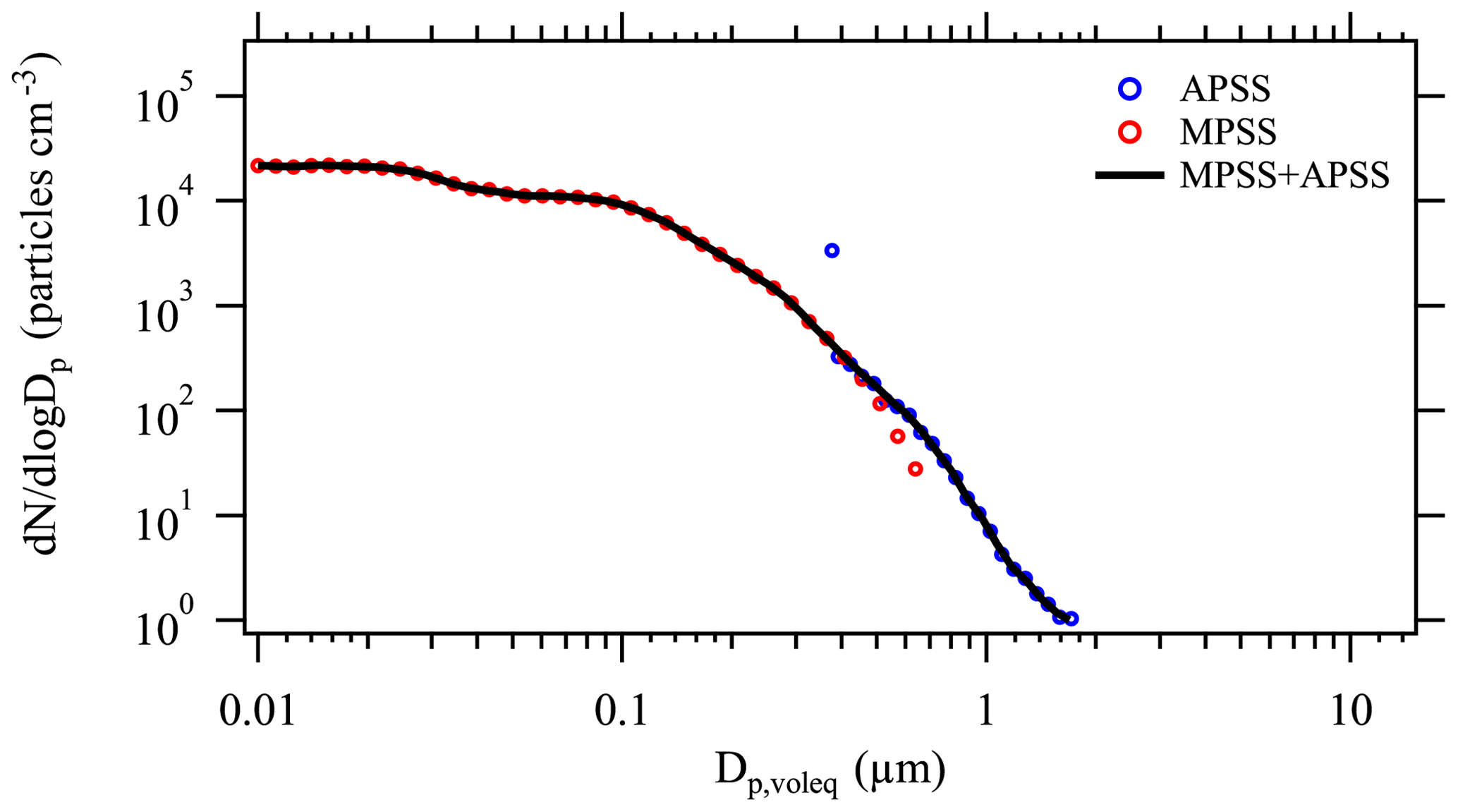
As one of the main objectives of this study is to provide a methodology for high-quality measurements of PM, this subsection goes into detail on how this is achieved when calculating PM from PNSDs. Deriving PM from the merged PNSDs of MPSS and APSS leads to high-time-resolution data of PM, which is an advantage over filter-based measurements that use gravimetric analyses to obtain PM mass concentrations. The following paragraph briefly describes the merging process, which can be found in detail in Costabile et al. (2017). First, the PNSD measured by the APSS, based on aerodynamic particle diameters (D_p,aer), was converted to a PNSD based on the volume equivalent particle diameters (D_p,voleq). The conversion assumed aged spherical particles in the fine mode (shape factor =1) as expected at urban background regions, as well as a size-dependent particle density (1.6 to 2 g cm⁻³). It was assumed that the particles in the fine-particle range were spherical or rather compact and that the mobility particle diameter is equal to the volume equivalent particle diameter. Figure 6 shows an example of the PNSDs measured by MPSS and APSS, including the indication of their overlapping size range from D_p,voleq 0.475 to 0.830 µm. For this size range, a combined PNSD was obtained by fitting a power-law function to the overlapping size range of the PNSDs of the APSS and MPSS. The two size distributions were merged by varying the PNSD expressed as dN∕(dlog(D)) after Khlystov et al.'s (2004) results. The fitting was constrained by an iterative procedure based on the minimization of the relative square difference between the PNSDs. The final PNSD covers the range from 0.01 to 10 µm volume equivalent particle diameter. The merged particle volume size distribution (PVSD) can be converted to particle mass size distribution (PMSD) by multiplying the former with the density of the particle of a certain size. The results of this procedure serve as a size distribution-derived PM reference with high time resolution which is necessary for the intercomparison against the mobile instruments.

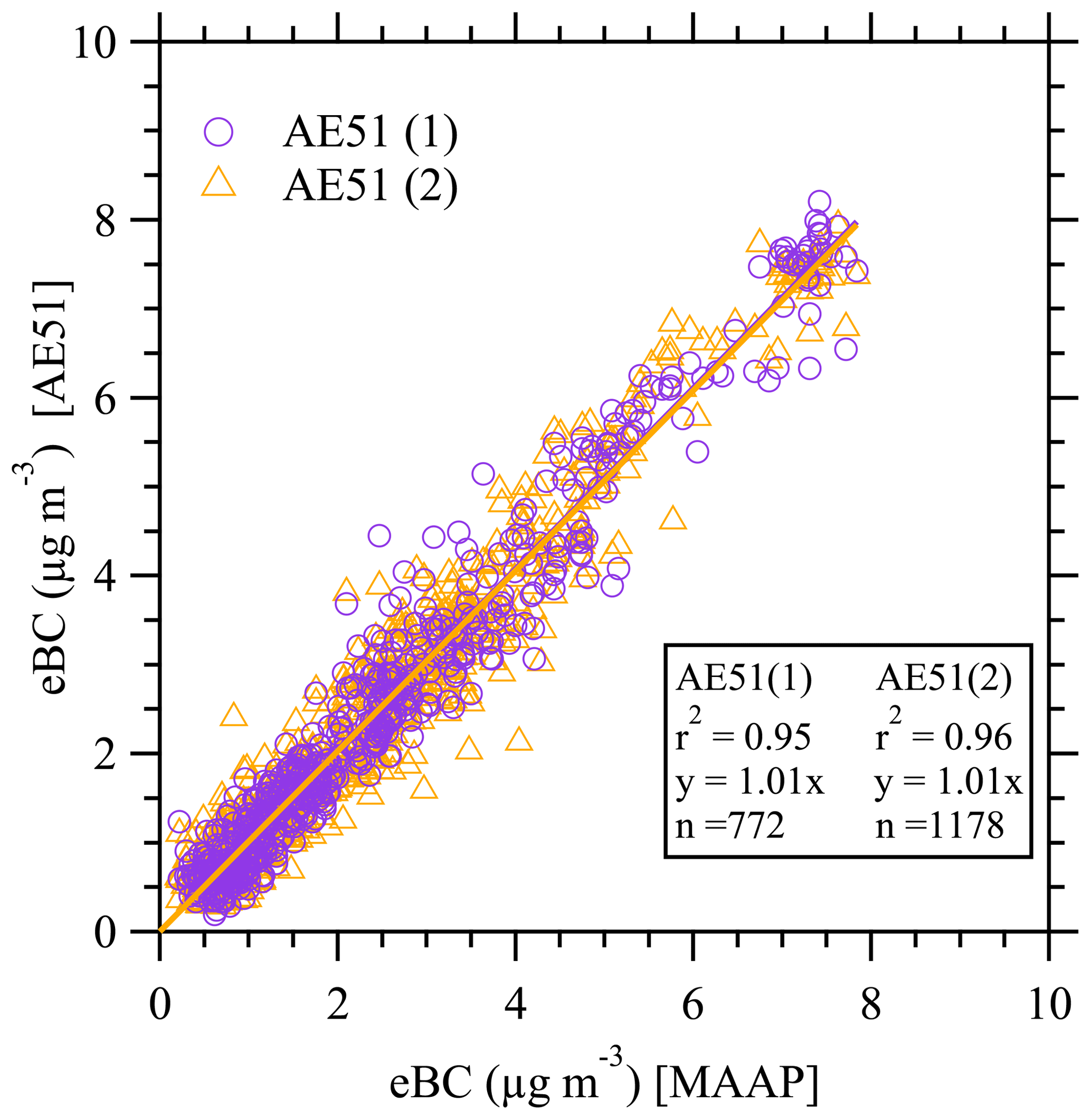
Figure 7 Correlation between the two AE51s (in 1 min average) aboard the aerosol backpacks against the reference absorption photometer MAAP during the intercomparison periods.

However, there are other options for the traceability of the mass concentration measurements. These options include online mass monitors, filter-based measurements, and chemical analyses. In this study, as reported by Costabile et al. (2017), the PM₁ derived from the MPSS size distribution was compared (r²=0.98, y=0.97x) against the PM₁ reconstructed from the MAAP and the Aerodyne aerosol chemical speciation monitor (ACSM). The PM_2.5 and PM₁₀ derived from this procedure were compared against the ones measured by a beta attenuation monitor (BAM) from an urban background station 3 km away. The PM_2.5 measurements compared well with each other (r²=0.86, y=1.048x), with no significant difference in the 24 h mass concentration. The agreement for PM₁₀ is lower (r²=0.73, y=0.88x), probably because of dust events, local resuspended dust, and differences of sources between the two stations. More information regarding the correlation of the fixed instruments against other methods employed either in the same station or in another nearby monitoring station is presented in the Supplement from Costabile et al. (2017).

3.3 Sufficiently long and frequent intercomparison periods between the mobile and fixed instruments

Having a fixed site with reference instruments provides the opportunity to check the performance of the mobile instruments in the field relative to the day-to-day changes (i.e., emissions, meteorology) within the study area. Performing sufficiently long and frequent intercomparisons against the reference instruments in the middle of a run further ensures the quality of the data from the mobile measurements. Furthermore, the intercomparisons harmonized the OPSS and MPSS+APSS at the reference site, which allows for the correction the OPSS PNSD per run based on the relative changes occurring in the study area. In this study, the runners stop by the fixed station for 30 min in the middle of each run for intercomparisons against the reference instruments. During the weekends the garden was closed and the reference station was inaccessible. For these times, the mobile measurements along a park area 460 m north of the aerosol container were used as a proxy for intercomparison against the reference instruments. This park area and the reference station were separated by a large green park inaccessible to vehicles. The results of these intercomparisons are discussed in the following paragraphs.

3.3.1 Intercomparison of the eBC mass concentrations from the mobile platform against the reference absorption photometer

For the eBC mass concentration measurements, the AE51 data were averaged per minute to compare with the MAAP. The AE51 data compared were within 5 % of the MAAP during the intercomparison periods (Fig. 7). This increases our confidence that the measured eBC mass concentrations are reliable for the entire route.

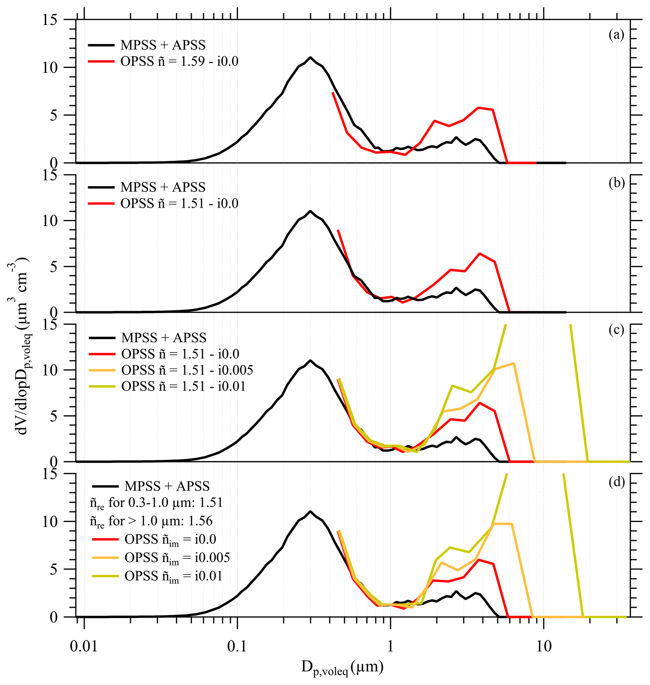
Figure 8 Demonstration of the complex refractive index correction done on the OPSS size distribution. In (a), the x axis for the OPSS is the optical diameter (D_p,opt). In the succeeding panels (b–d), the OPSS PVSD has been corrected and the x axes are geometric mean volume equivalent diameters (D_p,voleq).

3.3.2 Adjustment of the OPSS PNSD to the reference MPSS PNSD according to the complex refractive index (ñ)

This section provides a detailed and traceable method of calculating PM from the OPSS PNSD. As mentioned, the OPSS has been calibrated by the manufacturer with certified PSL particles of known sizes. These particles are spherical and nonabsorbing, with a complex refractive index (ñ) of 1.59–0.0i. This leads to inaccuracies of the optical PNSD from the OPSS, when used to measure ambient aerosol which has particles of various shapes, sizes, and ñ. Therefore, to derive PM mass concentrations from an OPSS, the optical PNSD must be adjusted with a ñ typical for the aerosol type of the study area. To achieve this, the OPSS must be compared consistently and frequently to a reference MPSS, which does not depend on particle optical properties such as ñ. Converting the optical particle number/volume size distribution of the OPSS by an aerosol-type-dependent ñ to an equivalent particle number/volume size distribution can yield reasonable results for the submicrometer size range compared to the MPSS-derived size distributions, assuming compact and spherical-like particles. Here, we demonstrate step-by-step the complex refractive index correction using the Mie theory on the OPSS data with the MPSS PNSD as reference using one of the 30 min intercomparison periods from a single run as an example.

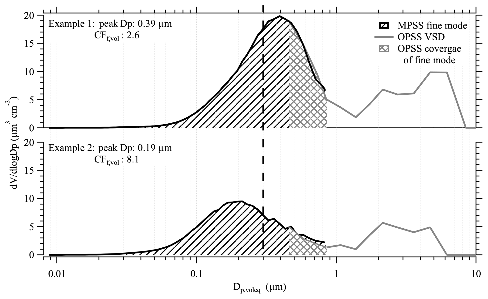
Figure 9 Dependence of the OPSS coverage of the fine mode on the variability of the fine-mode peak diameter.

Figure 10 Variability of the peak diameter and CF_f,vol color coded according to time of day.

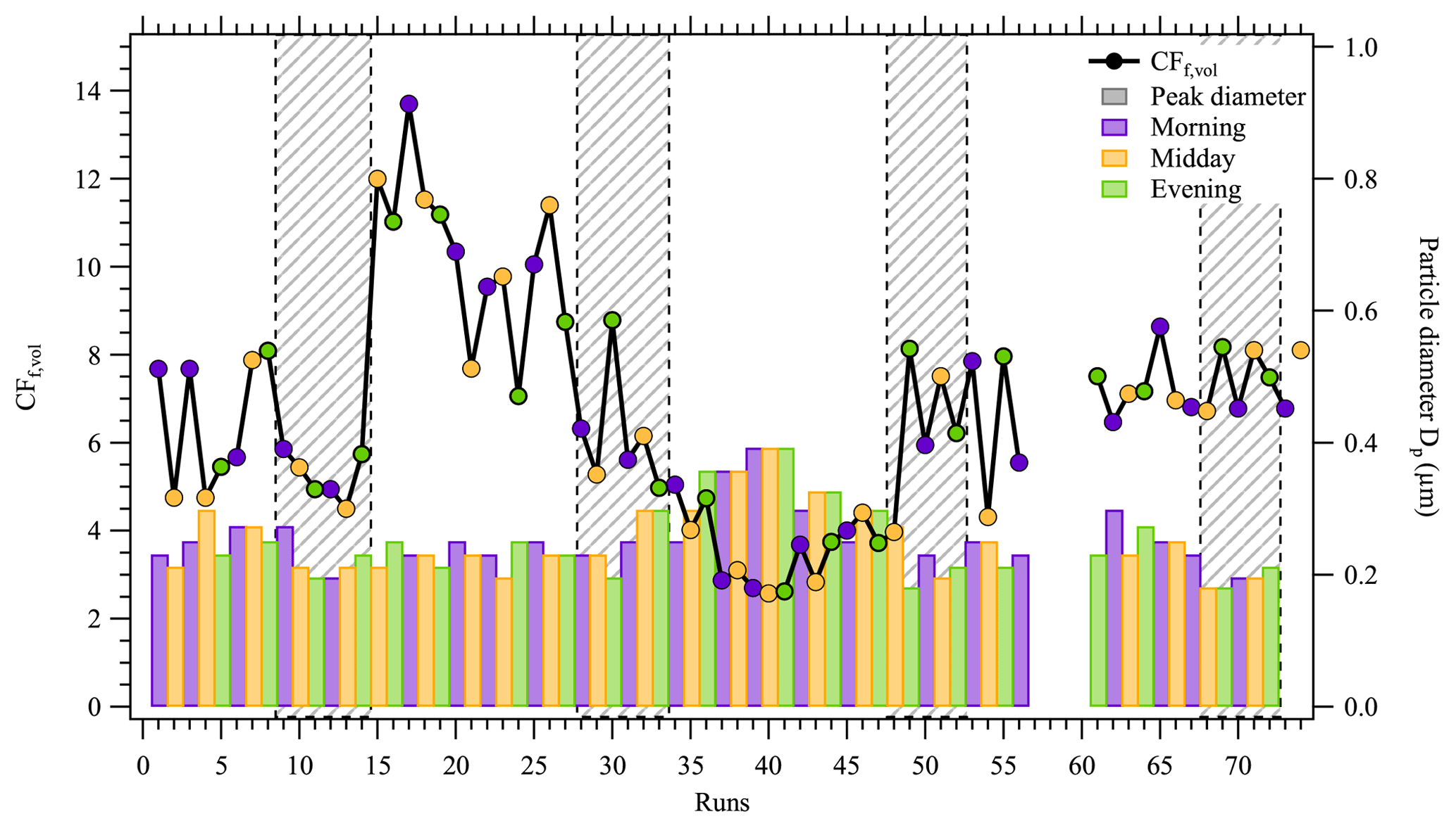
Figure 8a show the deviation between the particle volume size distributions (PVSD) of the OPSS from the MPSS before any correction. This deviation is due to the different diameters (optical for the OPSS and mobility for the MPSS) measured by the two instruments, as well as the inaccuracy of the OPSS due to ñ based on PSL. When the correction is applied using the Mie theory, the optical diameters are converted to geometric mean volume equivalent diameter. Figure 8b shows the effect of adjusting the real part (ñ_re) of the ñ to values typical of urban areas (1.51–0.0i) but keeping the imaginary part (ñ_im) zero. This yielded an OPSS PVSD in the submicrometer range that is reasonable when compared to the PVSD of the MPSS. Since the urban aerosol contains absorbing particles (BC, mineral dust, etc.), the imaginary part should not be zero. However, Fig. 8c shows that increasing the ñ_im results in artificial overestimation of the supermicrometer PVSD. This is due to two reasons: (i) the optical particle diameter of supermicrometer particles is sensitive to slight changes in the ñ_im of the refractive index, in the range from 0.0 to 0.01; and (ii) with increasing particle size of atmospheric aerosol particles, their shape also becomes more nonspherical, leading to unpredictable phase functions of the particle light scattering inside of the optics of the OPSS. Even for a latex-calibrated OPSS, this effect of nonspherical particles is not correctable since the refractive index correction by Mie theory is only possible for spherical particles.

In addition, the two instruments being compared have different operating principles (for the coarse-mode OPSS and APSS). It must be noted as well that the intercomparisons were such that the aerosol backpack and the reference systems are not in the same inlet and at different heights (aerosol backpack's inlet is ∼1.5 m above the ground while the fixed station inlet is ∼3.5 m a.g.l.), which could significantly influence the coarse-mode concentrations (higher coarse-mode particle concentrations are observed closer to the ground due to, for example, resuspension of particles).

Further attempts to correct the supermicrometer range by using a different ñ did not result in any significant improvement of the OPSS PVSD as shown in Fig. 8d. However, using size-resolved complex refractive indices (if they are known) is ideal as it might help in decreasing the difference between the PVSD of the OPSS and the MPSS. The results above show that the refractive index correction using Mie theory is not applicable to the supermicrometer size range.

From the result of the data experiments discussed above, the following were assumed in this study: ñ =1.51–0.007i and ñ =1.56–0.005i for particle diameters 0.3–0.8 µm and diameters larger than 0.8 µm, respectively. This yielded corrected D_p,voleq for the OPSS ranging from 0.46 to 12.02 µm after neglecting the first channel of the OPSS due to inaccuracy.

3.3.3 Determination of time-dependent fine-mode volume correction factors (CF_f,vol)

Another major limitation of the OPSS is that it measures only a fraction of the PNSD – in this case, only particles with optical diameter ranging from 0.3 to 10 µm. In Fig. 9, the comparison of the PVSD to the OPSS and MPSS shows that the OPSS misses the fine-mode volume peak (∼0.3 µm). This means that PM calculations from the OPSS PNSDs may lead to significant underestimation of the mass concentrations. In order to address this, relatively long and frequent intercomparison periods between the OPSS and the MPSS should be performed for each run. From these intercomparison periods, a correction factor (CF_f,vol) for the fine mode of the OPSS can be calculated based on its ratio with the MPSS fine mode (Eq. 1). This correction must be done on each run because of the dynamic nature of the fine-mode volume peak diameter (peak diameter from here on) and on the volume size distribution itself.

$$\begin{array}{}\text{(1)}& {\displaystyle }{\mathrm{CF}}_{\mathrm{f},\mathrm{vol}}={\displaystyle \frac{\text{MPSS fine mode}\left[\text{0.001–0.8}\mathrm{\mu }\mathrm{m}\right]}{\text{OPSS fine mode}\left[\text{0.4–0.8}\mathrm{\mu }\mathrm{m}\right]}}\end{array}$$

Figure 9 shows the VSDs of the MPSS and OPSS for two examples (high and low CF_f,vol). Fine-mode coverage by the OPSS varies with changes in the PVSD. Using the peak diameter as a proxy for these changes, as the peak shifts to the right the OPSS PVSD covers a larger portion of the fine mode (lower CF_f,vol) as compared to when the peak is located more to the left (higher CF_f,vol). This variability of the peak diameter measured by the MPSS depends on the local sources in urban areas. Since these local sources have a diurnal variability, so does the peak diameter.

Figure 10 summarizes the variability of the peak diameter from the MPSS (during intercomparison periods) along with the corresponding CF_f,vol for each run. There exists no significant pattern among the CF_f,vol, and hence it is necessary to correct each run individually. Since there are no other fixed monitoring stations with an MPSS along the rest of the route, the same correction factor was used to correct the fine mode of each data point along the whole route of one run. This assumption comes with limitations as it does not account for the likely differences of the aerosol sources along the entire route. A data experiment was performed comparing PVSDs obtained at an urban background station and at a roadside station in the city of Dresden, Germany, for the whole month of February 2017. For each site, effective correction factors (CF_f,vol) were calculated for each hour between 06:00 and 21:00 using the fraction covered by the OPSS as a proxy for the OPSS size distribution. For background station CF${}_{\mathrm{f},\mathrm{vol}}<\mathrm{2}$, which represented ∼50 % of the hourly data, there was excellent agreement between the paired background and roadside CF_f,vol values with 3 % mean bias and narrow variability (1σ=5 %). For higher CF_f,vol values the bias increased with increasing CF_f,vol and approached 20 % for CF${}_{\mathrm{f},\mathrm{vol}}>\mathrm{3}$ (background station having higher values) and the variability also increased (1σ=11 %). While caution must be used in extrapolating the Dresden data to other locations and conditions, these results provide a context for understanding the limitations when using a correction factor derived at a single location to represent the behavior along the entire route. For most cases, the impacts of location-dependent CF_f,vol values will be damped through the use of repeat runs although some concentration bias might remain.

Figure 11 Correlation between the PM_2.5 derived from the OPSS and MPSS+APSS.

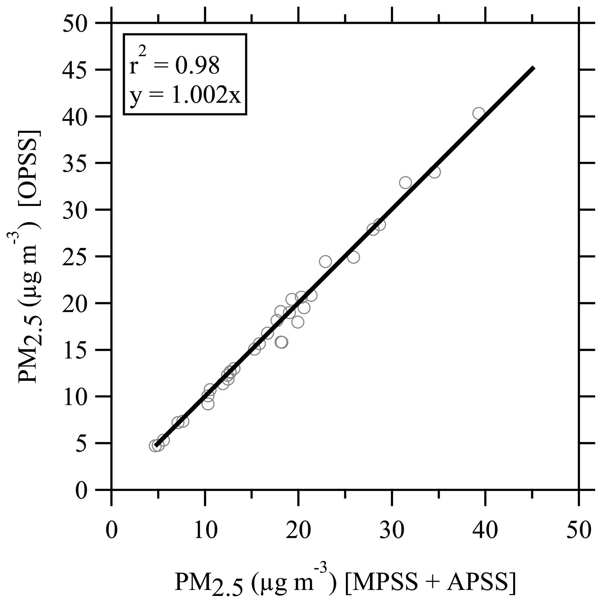
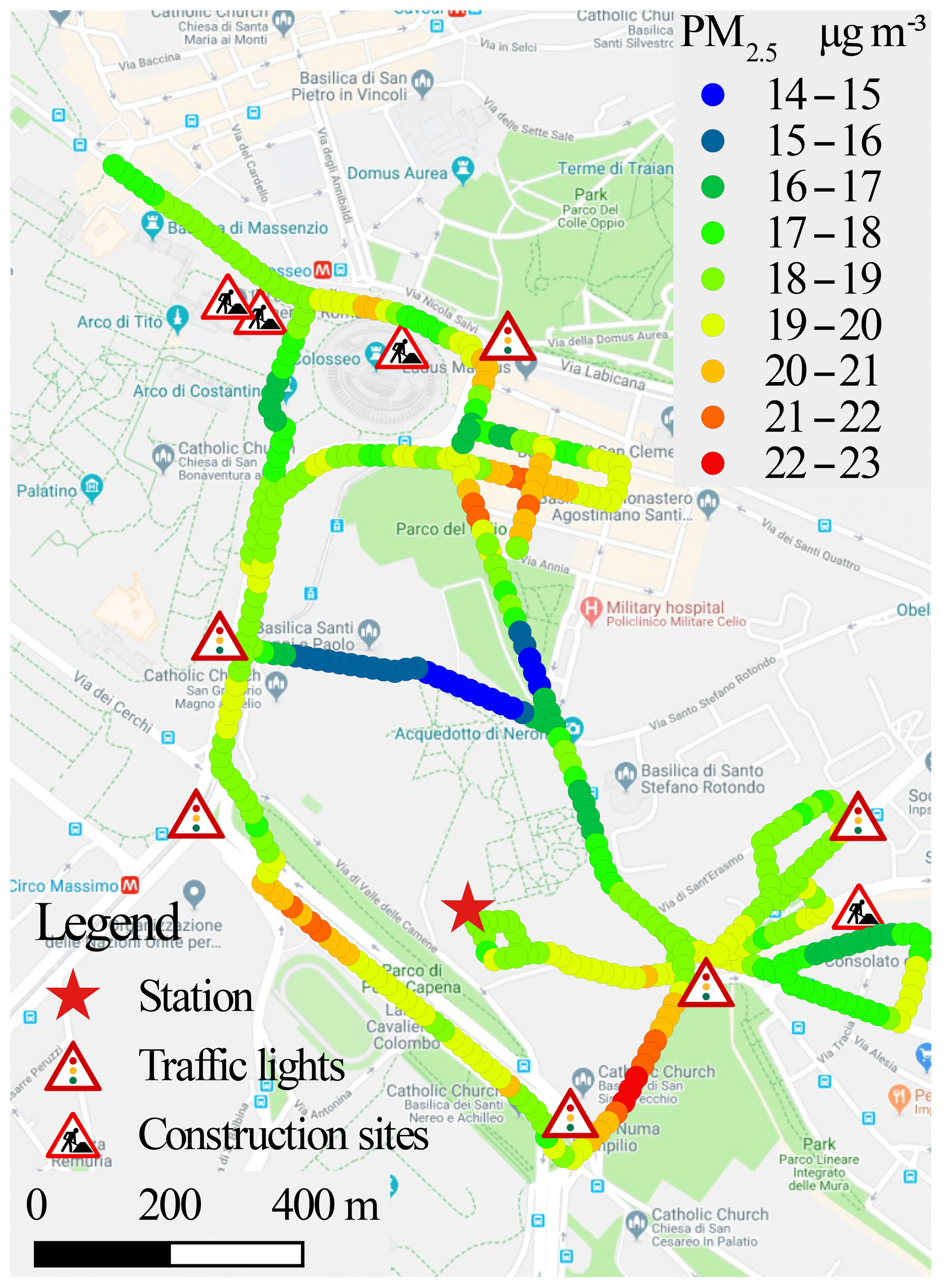
Figure 12 Overall spatial distribution of PM_2.5 along the fixed route during the CARE campaign. Map data © Google Maps 2015.

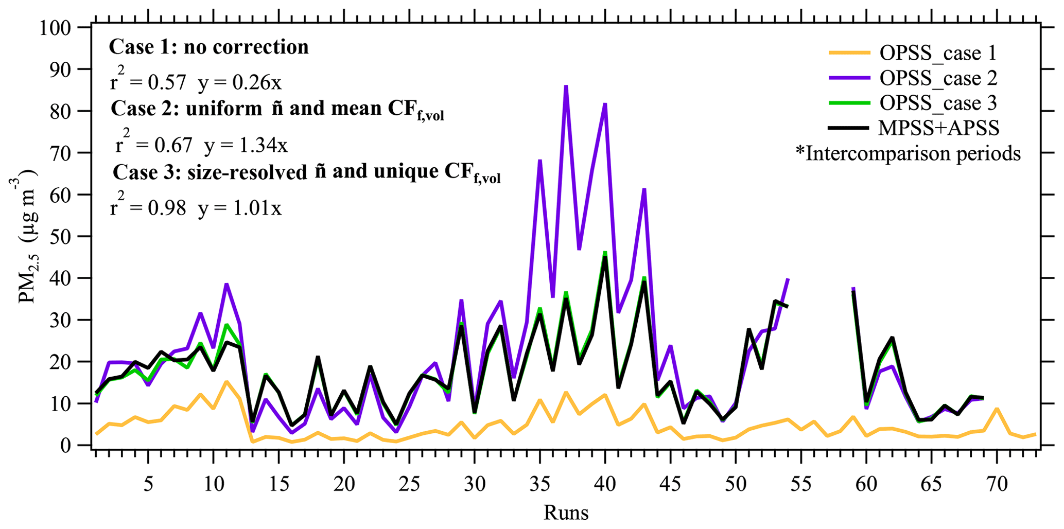
Figure 13 Illustration of the impact of data correction on the uncertainties of the PM_2.5 from OPSS.

3.3.4 Calculation of PM_2.5 mass concentration from the OPSS number size distribution

Once the CF_f,vol values have been determined for each run, PM mass concentrations can be calculated. The approach applied in this study was to correct PM₁ of the OPSS and add this absolute value to PM_1–2.5 and PM_1–10 to get PM_2.5 and PM₁₀, respectively. First, the OPSS PVSD was converted to a mass size distribution using a size-resolved particle density. Secondly, since the PM threshold is defined by D_p,aer, the equivalence of PM₁ and PM_2.5 to D_p,voleq, which serve as the new limits of integration, was determined following Eq. (2), which assumes spherical particles (shape factor =1):

$$\begin{array}{}\text{(2)}& {\displaystyle }{D}_{\mathrm{p},\mathrm{voleq}}=D_{\mathrm{p},\mathrm{aer}}\sqrt{{\displaystyle \frac{{\mathit{\rho }}_o}{{\mathit{\rho }}_{\mathrm{p}}}}},\end{array}$$

where ρ_o is the reference density (1 g cm⁻³) and ρ_p is the size-dependent particle density (1.6 and 2 g cm⁻³ for PM₁ and PM_2.5 and PM₁₀, respectively; see the Supplement of Costabile et al., 2017). Therefore, the particle mass size distributions were integrated from D_p,voleq 0.4–0.8, 0.8–1.7, and 0.8–7.8 µm for PM₁, PM_1–2.5, and PM_1–10, respectively. Linear interpolation was used to align the OPSS bin endpoints with these cutoff values. The PM₁ mass concentrations were corrected using Eq. (3), and PM_2.5 and PM₁₀ were calculated using Eqs. (4) and (5), respectively.

$$\begin{array}{}\text{(3)}& {\displaystyle }& {\displaystyle }\text{corrected}{\text{PM}}_{\mathrm{1}}={\mathrm{CF}}_{\mathrm{f},\mathrm{vol}}\times {\mathrm{PM}}_{\mathrm{1}}\text{(4)}& {\displaystyle }& {\displaystyle }{\text{PM}}_{\mathrm{2.5}}=\text{corrected}{\text{PM}}_{\mathrm{1}}+\text{PM}\left[\text{0.8–1.7}\mathrm{\mu }\mathrm{m}\right]\text{(5)}& {\displaystyle }& {\displaystyle }{\text{PM}}_{\mathrm{10}}=\text{corrected}{\text{PM}}_{\mathrm{1}}+\text{PM}\left[\text{0.8–7.8}\mathrm{\mu }\mathrm{m}\right]\end{array}$$

Figure 11 shows that the median PM_2.5 derived from the OPSS compares well with the one derived from the merged MPSS + APSS size distribution (r²=0.98, y=1.002x) during each intercomparison period. The resulting spatial distribution (Fig. 12) yielded reasonable results as well.

Furthermore, the impact of each correction procedure on the PM_2.5 value was investigated. Figure 13 shows that the deviation from the reference PM_2.5 decreases with the successive application of each step in the correction procedure. Without performing any correction on the OPSS data, PM_2.5 is underestimated by 74 %. When a refractive index correction is performed and a mean CF_f,vol is used, PM_2.5 values are 34 % higher than the reference. Finally, the deviation from the reference is significantly minimized when a size-resolved refractive index correction is used and a unique CF_f,vol is applied for each run.

The procedure outlined here to correct the size distributions (PNSD and PVSD) from the OPSS worked well with PM_2.5 but yields large uncertainties (>50 %) when higher size fractions are calculated, such as PM₁₀. As mentioned, this is attributed to the increasing irregularity in shape of larger particles, making the refractive index correction method based on the Mie theory ineffective. Therefore, other methods should be explored to correct the supermicrometer range of the OPSS size distribution.

4 Conclusions

A methodology to assure high-quality mobile measurement data of eBC and PM_2.5 mass concentrations was introduced and demonstrated using exemplary measurements from an intensive field study in Rome, Italy, on February 2017. The concept includes three main aspects: (a) the quality assurance of the mobile instruments and strategic design of the mobile measurements; (b) the quality assurance of reference instruments, including a fixed station in the mobile measurement route; and (c) sufficiently long and frequent intercomparison periods between the mobile and reference instruments as a basis for correcting the OPSS particle number size distributions. The concept proved effective in assuring the quality of the data from the mobile measurements. Performing collocated runs allowed for constant unit-to-unit intercomparison between mobile instruments leading to the detection of errors not flagged by the instruments operating in isolation. Fixed station measurements were used to frequently check the performance of the mobile instruments and to derive PM mass concentrations by referencing the OPSS to a mobility size spectrometer. This study also demonstrated that a correction of the OPSS data, using aerosol-type-dependent complex refractive indices and unique fine-mode volume correction factors, significantly improved calculated PM_2.5 mass concentrations. However, large uncertainties were observed for the PM₁₀ mass concentration.

Data of this quality can be beneficial to increase the accuracy of exposure estimates as well as in validation of microscale models. Moreover, the high-spatial-resolution data can prove valuable for policy-makers and urban planners in developing strategies to mitigate air pollution.

Appendix A: Mobile measurement platform

The mobile aerosol measurements were performed using a mobile platform (the “aerosol backpack”) that was designed to be easily carried by a pedestrian as shown in Fig. A1. A 1 m long stainless-steel inlet protrudes from the top of the backpack with a GPS device resting on a metallic plate on top. Ambient air is sampled through this inlet and then splits into two channels: one leading to an absorption photometer to measure eBC after passing a silica-based aerosol diffusion dryer and other leading to the optical particle size spectrometer. The absorption photometer used in this study is the AethLabs microAeth^® model AE51. It determines eBC mass concentrations based on the attenuation of light (880 nm) passing through a particle-loaded filter and assuming a mass attenuation cross section (12.5 m² g⁻¹). The instrument operates on a time base of 1 s and a flow rate of 100 mL min⁻¹. Since the AE51 has been known to be sensitive to sudden changes in humidity, the aerosol first passes through a dryer which is a Perma Pure membrane within an aluminum mesh. This mesh is then surrounded by silica gel granules. This setup is housed in a small sealed box to keep the silica gel granules dry and avoid leaks. The optical particle size spectrometer employed here is the TSI OPSS model 3330, which provides an optical particle number size distribution (PNSD) from 0.3 to 10 µm divided into 16 channels. The aerosol enters the instrument with a flow of 1 L min⁻¹ and is led into a detection chamber, where it crosses a vertically polarized laser beam with a wavelength of 660 nm. The light scattered by the particle is focused by a 120^∘ spherical collecting mirror to the photodetector (more details in the instruments user manual). The intensity of the light pulse and counting rate are used to size and count the particles, respectively. The aerosol sampled by the OPSS is not dried, which may influence the measurements in humid environments. The data acquisition is controlled and synchronized by a microcomputer which is powered by a battery package. The same battery package powers the AE51 and GPS while the OPSS has its own source. All these instruments (except the GPS) are secured inside a waterproof, hard case backpack.

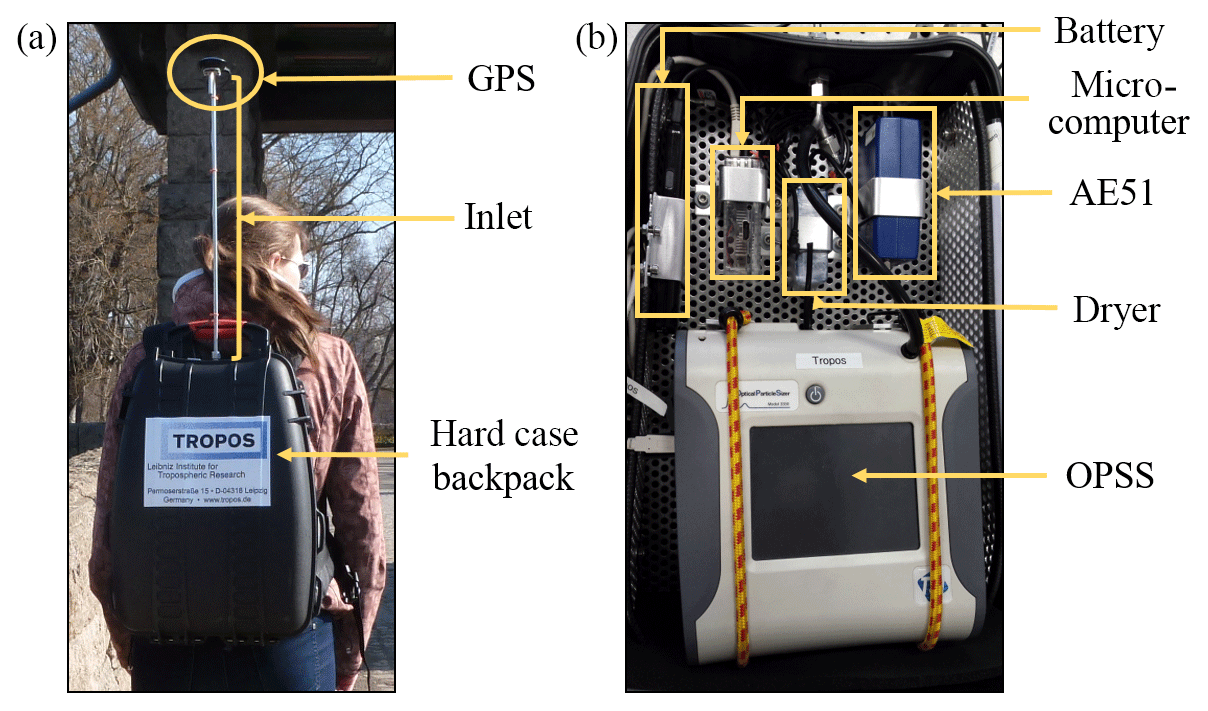
Figure A1 The TROPOS aerosol backpack from the outside (a) showing the GPS unit, inlet, and entire backpack; and from the inside (b) showing the different components and main instruments: AE51 and OPSS. Image source: TROPOS (2016).

Appendix B: Fixed reference station

A fixed reference measurement station was set up within a garden with restricted traffic and public access and was approximately 100–400 m away from the major roads. The station is a mobile laboratory (AEROLAB), designed for ambient aerosol and gas measurements with controlled indoor conditions. The sampling system consisted of a PM₁₀ inlet followed by an aerosol diffusion dryer, conditioning the relative humidity level below 40 %. The aerosol then passed through an isokinetic splitter, distributing the aerosol to the different instruments, including the calibrated and quality-assured reference instruments used for this study: a MAAP for eBC (multiangle absorption photometer, model 2012, Thermo, Inc., Waltham, MA USA), a TROPOS-type MPSS for the PNSD (Wiedensohler et al., 2012), and an APSS (aerodynamic particle size spectrometer, model 3321, TSI Inc., Shoreview, MN USA).

MAAP determines the aerosol light absorption coefficient at a wavelength of 637 nm (Petzold and Schönlinner, 2004) with 1 min time resolution. The mass concentration of eBC is then internally calculated, using a mass absorption cross section of 6.6 m² g⁻¹. The MPSS classifies electrical particle mobility in the range 0.01 to 0.80 µm (mobility diameter, D_p,Mob). Using the standardized bipolar charge distribution, the PNSD can be calculated (Wiedensohler, 1988). The uncertainty of the reference instrument in terms of the integral number concentration is smaller than 10 % and in terms of sizing is smaller than 3 % (Wiedensohler et al., 2018). The APSS determines the PNSD using the time of flight in an accelerated flow to determine the aerodynamic particle diameter. The aerodynamic particle size range covered by the APSS is approximately 0.7 to 10 µm for atmospheric applications. Both the MPSS and the APSS were operated with a time resolution of 5 min.