Multiple technical observations of the atmospheric boundary layer structure of a red-alert haze episode in Beijing

The study and control of air pollution involves measuring the structure of the atmospheric boundary layer (ABL) to understand the mechanisms of the interactions occurring between the atmospheric boundary layer and air pollution. Beijing, the capital of China, experienced heavy haze pollution in December 2016, and the city issued its first red-alert air pollution warning of the year (the highest PM_2.5 concentrations were later found to exceed 450 µg m⁻³). In this paper, the vertical profiles of wind, temperature, humidity and the extinction coefficient (reflecting aerosol concentrations), as well as ABL heights and turbulence quantities under heavy haze pollution conditions, are analyzed, with data collected from lidar, wind profile radar (WPR), radiosondes, a 325 m meteorological tower (equipped with a 7-layer ultrasonic anemometer and 15-layer low-frequency wind, temperature, and humidity sensors) and ground observations. The ABL heights obtained by three different methods based on lidar extinction coefficient data (H_c) are compared with the heights calculated from radiosonde temperature data (H_θ), and their correlation coefficient can reach 72 %. Our results show that H_θ measured on heavy haze pollution days was generally lower than that measured on clean days without pollution, but H_c increased from clean to heavy pollution days. The time changes in friction velocity (u_*) and turbulent kinetic energy (TKE) were clearly inversely correlated with PM_2.5 concentration. Momentum and heat fluxes varied very little with altitude. The nocturnal sensible heat fluxes close to the Earth surface always stay positive. In the daytime of the haze pollution period, sensible heat fluxes were greatly reduced within 300 m of the ground. These findings will deepen our understanding of the boundary layer structure under heavy pollution conditions and improve the boundary layer parameterization in numerical models.

1 Introduction

Air pollution has an important impact on human health, weather, climatic patterns and the ecological environment (Seinfeld and Pandis, 1997; Brook et al., 2004; Ding et al., 2013; Wang et al., 2014; Zhang et al., 2015a). The pollutants emitted as a result of human activities are mainly confined to the atmospheric boundary layer (ABL), which is the lowest part of the troposphere and is approximately 1–2 km from the ground. In particular, fog and haze, which have a strong influence on visibility and air quality levels, mainly occur in the ABL (Cao et al., 2004; Chan and Yao, 2008; Fu et al., 2008; Liu et al., 2012). Because the formation, evolution and diffusion of air pollutants are closely related to ABL structures and turbulence characteristics (Zhang et al., 2012; Wei et al., 2018), research on the ABL is important for understanding air pollution mechanisms and for developing pollution control strategies. On the other hand, the relationships between the ABL and atmospheric pollution are very complex and involve multiscale nonlinear physical and chemical processes; thus, both theoretical research and numerical simulations have encountered difficulties (Sun et al., 2013; Huang et al., 2014; Wang et al., 2015; Miao et al., 2018). Therefore, it is very necessary to obtain first-hand information from observation experiments. Because of the Earth's rotation, the ABL presents strong diurnal variation, leading to the formation of many different layers in the boundary layer. The mixing layer accounts for a large proportion of the ABL in the deep convective boundary layer, and, at present, the height of the mixing layer is equivalent to the height of the ABL. Pollutants emitted into the ABL can reach a certain height through turbulent vertical mixing processes (Emeis and Schäfer, 2006), making it possible to determine the ABL height from the concentration of pollutants. The top of the mixing layer exhibits a capping inversion. Due to a change in the surface net radiation occurring at night, a stable boundary layer begins to form at night because of the cooling effect of the ground surface and the surface inversion layer is nearest to the ground. The nocturnal stable boundary layer is often accompanied by a residual layer that maintains the characteristics of the daytime mixing layer (Stull, 1988). The ABL height is closely related to air pollution, but it is not the only factor that shapes air quality. Pollution conditions are also affected by wind speeds, emissions, chemical processing, etc. (Schäfer et al., 2006; Geiß et al., 2017). Some previous work has compared ABL heights based on lidar and radiosonde data, and the correlations between them are stronger under unstable conditions (Emeis and Schäfer, 2006; Martucci et al., 2006).

Regarding air pollution, many observational experiments have been conducted internationally, especially with reference to air pollution in the ABL over urban areas (i.e., the urban boundary layer). Examples of such projects include European Cooperation in the Field of Scientific and Technical Research, abbreviated as COST715 (Fisher et al., 2001); URBAN 2000, a major urban tracer and meteorological field campaign conducted in Salt Lake City, UT, in October 2000 (Allwine et al., 2002); Joint Urban 2003, a field experiment conducted in October 2003 in Oklahoma City, OK (Wang et al., 2007); MIRAGE 2006, Megacity Impacts on Regional and Global Environments (Lance et al., 2012); and SURF, the Study of Urban impacts on Rainfall and Fog/haze (Liang et al., 2018).

A meteorological tower serves as one of the best platforms from which to detect the ABL structure under conditions of atmospheric pollution (Quan and Hu, 2009; Sun et al., 2015; Ren et al., 2018). Although the height of such a tower is limited, the boundary layer is often stable when heavy pollution occurs and the ABL height is low, so it is easy to measure from a tower. Conventional meteorological and turbulence instruments installed at different heights above a meteorological tower can obtain information on stable boundary layer structures and turbulence diffusion parameters (Katul et al., 1995). Traditional detection methods include tethered balloons, radiosondes and wind profile radar (WPR) tools, which can detect higher heights (Grimsdell and Angevine, 1998; Andreas et al., 2000; Kalapureddy et al., 2007; Li et al., 2015; Han et al., 2018). In recent decades, aerosol laser radar (lidar) has been used increasingly extensively. It can be used to retrieve the vertical distribution of particles from lidar backscattering data (Wang et al., 2012; Summa et al., 2013; Quan et al., 2013; Bravo-Aranda et al., 2017). It is impossible to obtain information on the boundary layer structure and on the interrelationships between pollutants found in atmospheric pollution (especially in heavy haze) unilaterally by means of the above-mentioned technical techniques, and it is necessary to carry out comprehensive observations simultaneously.

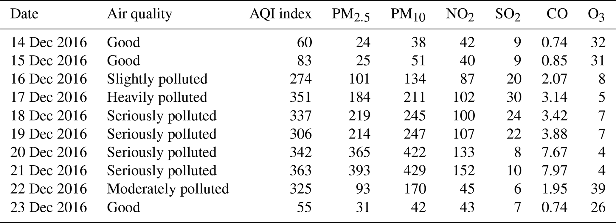
From 14 to 22 December 2016, Beijing, the capital of China, experienced a period of severe haze pollution. The government issued its highest air pollution warning (red alert) during this period. Beijing is a densely populated city covering an area of approximately 396 km² (see Fig. 1b). Despite strong pollution control measures taken by the government, the average PM_2.5 concentration per hour rose from 20 µg m⁻³ to more than 450 µg m⁻³ (see Table 1) in just 5 d. What are the mechanisms of episodes of such severe air pollution? Addressing this question requires conducting a comprehensive and in-depth analysis of weather conditions, pollutant emissions, regional transport processes, physicochemical transformation mechanisms and interactions between haze and boundary layer structures (Huang et al., 2014; Sun et al., 2014; Ding et al., 2016). Some previous studies have been conducted on haze events in the Beijing area (Li et al., 2017; Sheng et al., 2018; Wang et al., 2018), on the physical and chemical mechanism analyses especially, based on comprehensive observation data from tall towers (Sun et al., 2006; Guo et al., 2016).

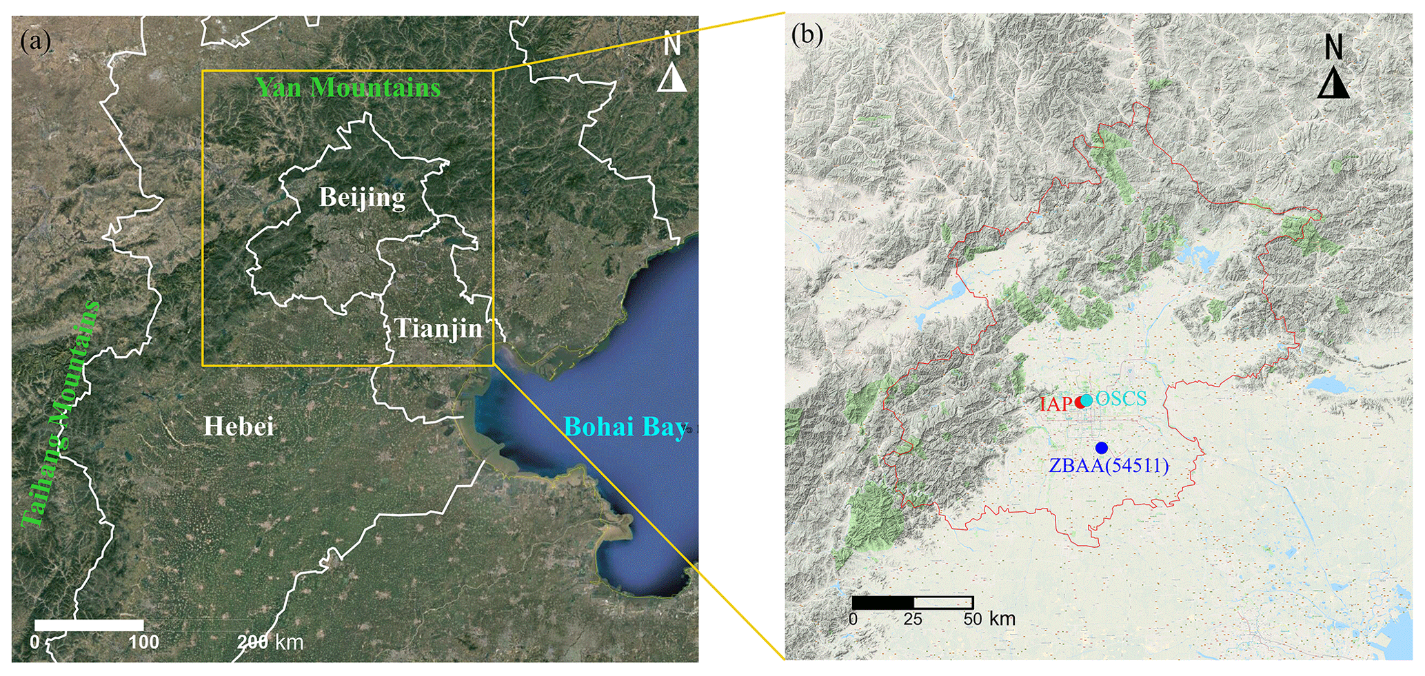
Figure 1 Local topography of Beijing and of its surrounding area (a). The locations of observation sites in Beijing (b) – red circle: IAP (lidar); blue circle: ZBAA radiosonde observation station; cyan circle: pollution observation station (OSCS), which is positioned approximately 2 km northeast of the lidar. Beijing is a densely populated city covering an area of approximately 396 km². Both maps were obtained from © Google Maps.

Table 1 Daily average data for six major air pollutants in Beijing measured during a period of heavy pollution from 14 to 23 December 2016: PM_2.5, PM₁₀, NO₂, SO₂ and O₃ (µg m⁻³); CO (mg m⁻³). Data sources: http://beijingair.sinaapp.com/ (last access: 28 August 2019). According to the “Technical Specification for Air Quality Index (HJ 633-2012)” issued by China's National Environmental Protection Agency, air pollution levels can be divided into five levels based on PM_2.5 concentrations, i.e., good (0–75 µg m⁻³), slightly polluted (75–115 µg m⁻³), moderately polluted (115–150 µg m⁻³), heavily polluted (150–250 µg m⁻³) and seriously polluted (>250 µg m⁻³).

The purpose of this paper is to use multiple technical observational datasets to analyze the vertical structure and turbulence properties of the atmospheric boundary layer during heavy pollution, particularly when comparing the differences in the boundary layer height obtained by different methods and calculation schemes. The observation data are mainly from high meteorological towers, lidar, WPR and radiosondes, as well as related satellite images, surface meteorology and air pollution observations. After briefly introducing the background weather conditions, observation sites, instruments and data, we analyze the vertical distribution of wind, temperature, humidity, and extinction coefficients; the multilayer measurement of turbulence on a 325 m high tower; and the characteristics of boundary layer height in the process of severe air pollution development. Further research work in the future is also discussed.

2 Observation sites, instruments and data

The ABL observation data used for this paper mainly cover three locations in Beijing. The first area is located at the Institute of Atmospheric Physics (IAP) of the Chinese Academy of Sciences, where there is a 325 m high meteorological tower and a lidar. The second area is positioned approximately 600 m away from the east side of this tower where a WPR system is based. The third area is the observatory of the Beijing Meteorological Bureau, which is approximately 20 km away from the tower. Conventional ground meteorological observations and radiosonde data from the WMO station are used (ZBAA in Fig. 1b). The above observation sites are shown in Fig. 1b. The topography around Beijing is also given in Fig. 1a. We use local station time in this work, and the observational instruments and data employed are as follows.

• 1.

  The IAP's meteorological tower is positioned 49 m above sea level, is 325 m tall and is located at (39^∘58^′ N, 116^∘22^′ E) between the Beijing North Third Ring Road and North Fourth Ring Road. A total of 15 observation platforms (at 8, 15, 32, 47, 65, 80, 103, 120, 140, 160, 180, 200, 240, 280 and 320 m) are set up on the tower, and wind speed (MetOne, USA), wind direction (MetOne, USA), temperature (HC2-S3, Switzerland) and humidity (HC2-S3, Switzerland) observation instruments are mounted onto each platform. In addition, seven sets of three-dimensional ultrasonic anemometers (Wind Master, Gill, USA) and water vapor and carbon dioxide analyzers (LI-7500,USA) are installed on the tower (at 8, 15, 47, 80, 140, 200 and 280 m). All turbulence data sampling frequencies are set to 10 Hz. All of the tower data are averaged for 20 min. A detailed description of the meteorological tower can be found in Al-Jiboori and Fei (2005) and Chen et al. (2018) and on the website (http://view.iap.ac.cn:8080/imageview/, last access: 28 August 2019).

• 2.

  The extinction coefficients were measured by a lidar system (AGHJ-I-lidar, China) installed underneath the 325 m tower. The lidar can provide backscattering signals at wavelengths of 532 and 355 nm at a vertical resolution of 7.5 m and a temporal resolution of approximately 5–10 min. The blind zone of the lidar is about 90 m, and lidar signals are not reliable below 250 m because of the incomplete transmitter–receiver overlap. Due to technical failures, lidar data are missing for 11:00 LT on 19 December to 09:00 LT on 20 December 2016.

• 3.

  Wind speeds and wind directions were also monitored by means of WPR (Airda3000, China) during red-alert pollution periods. In this paper, the temporal resolution of WPR is set to 5 min and the vertical resolution is set to 50 m below 1000 m and 90 m above 1000 m.

• 4.

  High-resolution vertical profile radiosonde data collected twice daily (08:00 and 20:00 LT Beijing time) were retrieved from the University of Wyoming's website (http://weather.uwyo.edu/, last access: 28 August 2019) for Beijing's meteorological observatory station, which is named ZBAA in international code (Fig. 1b). Surface visibility and other normal meteorological variables were routinely measured with a temporal resolution of 0.5 h in ZBAA.

• 5.

  Surface measurements of six kinds of air pollutants (PM_2.5, PM₁₀, NO₂, SO₂, CO and O₃) with a temporal resolution of 1 h can be found on the official website of the Beijing Environmental Protection Agency (http://beijingair.sinaapp.com/, last access: 28 August 2019). The data used in this paper were collected from the environmental monitoring station (Olympic Sports Center Station) positioned closest to the tower (approximately 2 km to the northeast).

3 Results and discussion

3.1 Surface observations of haze and meteorological conditions

From 14 to 22 December 2016, complete haze pollution was observed in the Beijing area (see Table 1). The generation, accumulation and elimination of PM_2.5 were recorded. We can see that from 20 to 21 December, the hourly average PM_2.5 concentration was almost maintained at approximately 400 µg m⁻³ over 48 h, which greatly exceeded the air pollution limits (i.e., 250 µg m⁻³) set by China's State Environmental Protection Administration. Figure 2 shows the concentration time series for PM_2.5, wind speed and direction, temperature, relative humidity (RH), surface pressure and visibility for this period of heavy haze pollution.

Generally, visibility serves as a representative index of air quality and atmospheric diffusion capacity (Zhang et al., 2015b). Figure 2 shows that when the concentration of PM_2.5 increased to high levels, visibility quickly deteriorated. Visibility on clean days was largely measured as greater than 10 km, and when the PM_2.5 concentrations reached approximately 200–300 µg m⁻³, the visibility decreased to 2–5 km. Even when PM_2.5 reached approximately 400 µg m⁻³, visibility dropped sharply to 1 km or to hundreds of meters. The surface pressure results suggest that air pressure levels decreased from approximately 1035 to 1023 hPa, and, in general, Beijing was controlled by a weak high-pressure system during the pollution episode. The RH taken from ground observations shows significant diurnal variations and an obvious anticorrelation between RH and temperature. From 20 to 21 December, the diurnal variation in temperature and relative humidity in heavy pollution was greatly suppressed, and a further analysis of MODIS images (see Fig. 3) during this period shows that the pollution process was indeed accompanied by fog, while pollution formed in the south-central area of Hebei Province on 15 December 2016 and then spread across the whole Beijing–Tianjin–Hebei area on 18 December. Stratiform clouds appeared in areas surrounding Beijing on 21 December, but due to the high concentrations of pollutants (PM_2.5 values approaching 400 µg m⁻³), mixed fog and haze appeared in Beijing. During the day, pollutants can scatter more solar radiation, while the ground receives less solar radiation, leading to the suppression of diurnal variations in temperature and relative humidity on the ground (Gao et al., 2015). An increase in RH occurs due to a decrease in temperature but is also the result of a surge in water vapor. For example, in the early morning, temperature differences observed between 17 and 20 December were minor, and the RH on 17 December was approximately 80 %, while the RH in the early morning of 20 December reached nearly 100 %, indicating an increase in water vapor levels in the Beijing area at this time. The surface wind speed during the pollution episode fell to almost less than 2 m s⁻¹ and can be basically regarded as a stagnant weather system dominating ABL processes and resulting in poor air quality. From Fig. 2, we can see that there were cold fronts (strong northwesterly winds) on both 15 and 22 December, which advected pollutants away, resulting in good air quality. Between the fronts, PM_2.5 levels slowly increased, as the air was stagnant (weak and variable winds in between) and the pollutants that were emitted locally slowly built up. The wind direction also seemed to be cyclical on each day in response to local mountain valley circulation around Beijing (Hu et al., 2005). According to other studies, stronger northerly winds occurring in the winter are the main mechanism through which pollution is removed, leading to good air quality (Sheng et al., 2018).

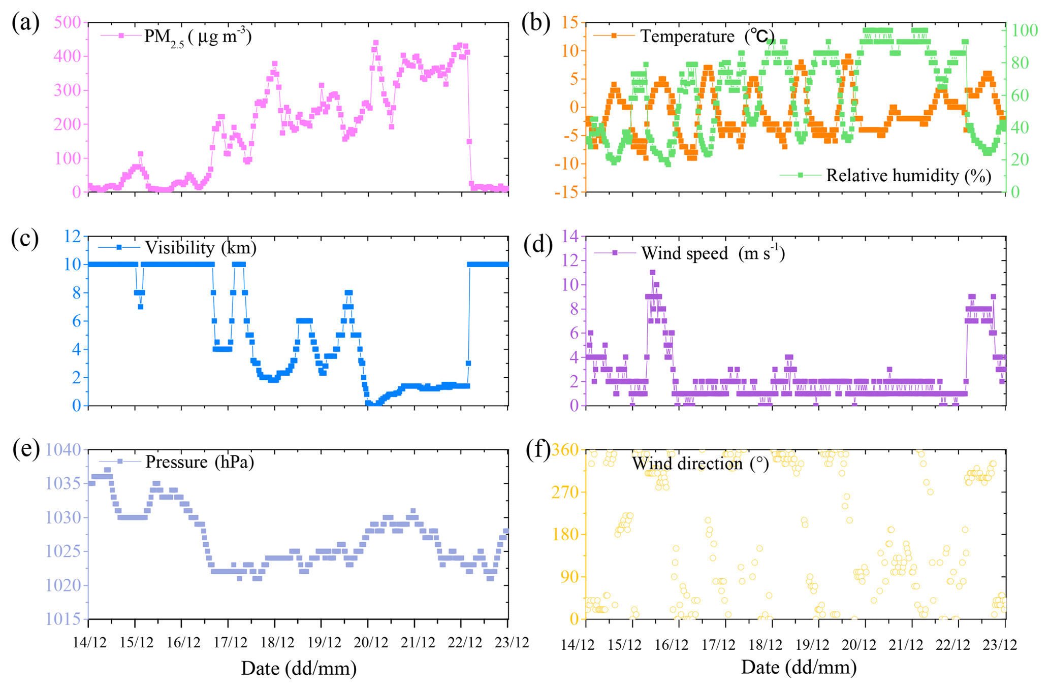
Figure 2 Time series of ground level PM_2.5 (a), relative humidity and temperature (b), visibility (c), wind speed (d), surface pressure (e), and wind direction (f) from 14 to 22 December 2016. The units for these meteorological parameters are as follows: micrometers per cubic meter, percentage, degrees Celsius, kilometers, meters per second, hectopascals and degree, respectively.

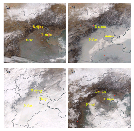
Figure 3 MODIS images of the Beijing–Tianjin–Hebei region on 15 December (a), 18 December (b), 21 December (c) and 22 December (d). Both maps were obtained from the following website: https://worldview.earthdata.nasa.gov/ (last access: 28 August 2019).

3.2 Boundary layer heights observed by lidar

The most basic definition of the ABL height is the height at which the influence of the Earth's surface on the lower troposphere disappears. This influence applies not only to conventional meteorological elements but also to turbulence quantities and even more for substances in the atmosphere such as aerosols, water vapor and nonreactive tracer gases (Seibert et al., 2000). Levels of various pollutants and water vapor in the ABL are much higher than those found in the free atmosphere, and therefore there is often an obvious aerosol concentration gradient between the boundary layer and the free atmosphere. The extinction coefficient reflects the degree of aerosol particle scattering from lasers in the atmosphere (Boers and Eloranta, 1986). Thus, the ABL height can also be estimated from the extinction coefficient gradient. We used three popular methods – the gradient method (lidar_gra) (Flamant et al., 1997), the standard deviation method (lidar_SD) (Hooper and Eloranta, 1986) and the wavelet method (lidar_wav) (Cohn and Angevine, 2000; Davis et al., 2000; Brooks, 2003) – to extract boundary layer heights from extinction coefficients (continuous Haar wavelet transformation was used in this paper, taking dilation parameter a=6). The ABL height determined by lidar is represented by H_c. In this study, the lidar_gra method applies the height of the atmosphere at which the gradient of the lidar extinction coefficient reaches its most negative value. The standard deviation of the extinction coefficient reflects the degree of lidar echo signal dispersion at different heights. The top of the planetary boundary layer constitutes the intersection between air in the boundary layer and the free atmosphere, which leads to a strong signal change at the top of the boundary layer. We define the height of the maximum standard deviation of signals as the ABL height. The lidar_wav method can also be used to detect abrupt changes in signals, so we use the Haar wavelet and take the height at which the wavelet coefficient is at its highest value as the height of the ABL. These methods are used to find the abrupt change in the extinction coefficient occurring at the top of boundary layer, though they present their own limitations.

Generally, the atmospheric boundary layer can be divided into a daytime convective mixing layer and a nighttime stable boundary layer. In the morning, the well-mixed convective boundary layer (CBL) is growing and often reaches its maximum height in the early afternoon. In the afternoon, the CBL gradually transforms into a neutral boundary layer. Figure 4 illustrates the evolution of ABL heights measured with lidar and radiosondes.

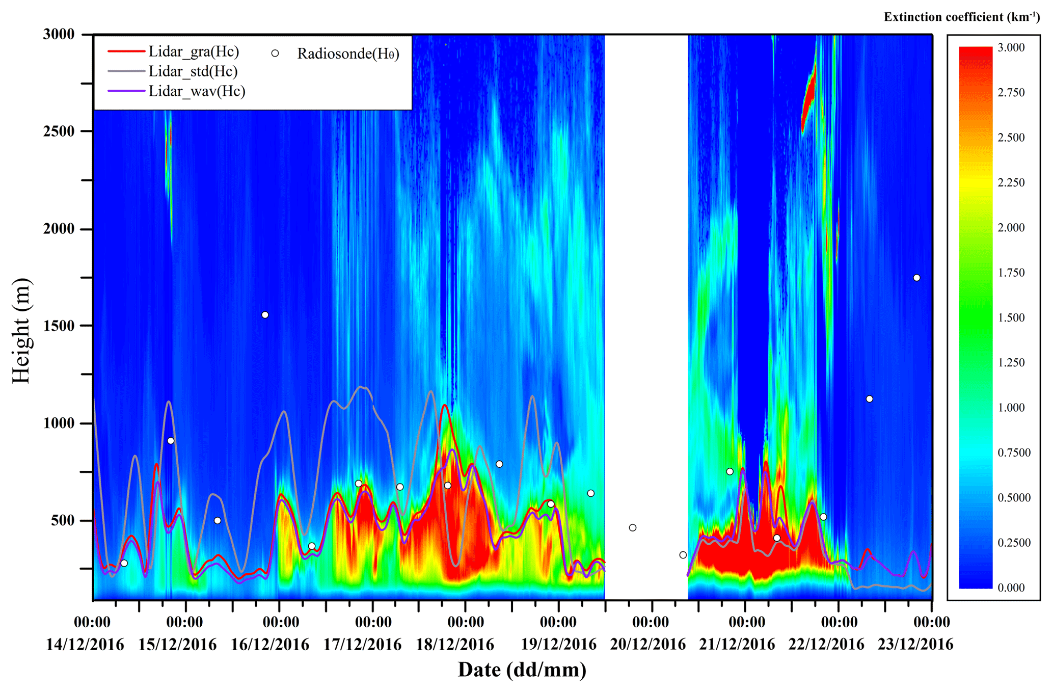
Figure 4 Temporal and spatial variations in the extinction coefficient (shaded, unit: km⁻¹) from 14 to 23 December 2016 and ABL heights (m) determined with different instruments. The red line (lidar_gra), grey line (lidar_SD) and purple line (lidar_wav) represent ABL heights determined by the lidar using the gradient method, the standard deviation method and the wavelet method, respectively. White points: ABL height determined by radiosondes. It should be noted that the blank part of the extinction coefficient can be attributed to a technical failure and that lidar data for 11:00 LT on 19 December to 09:00 LT on 20 December are missing.

The determination of the ABL height by means of the lidar method is based on the vertical profiles of the extinction coefficient or the aerosol concentration. When concentrations of PM_2.5 are high, the weakening effects of aerosol particles on lasers are stronger. ABL heights determined by lidar_gra and lidar_wav were almost the same, with a correlation coefficient of nearly 95 %. From 16 to 18 December and from 20 to 21 December, the ABL heights were approximately 500–750 m. Furthermore, the ABL height determined by the lidar_SD method was slightly higher than that derived from both methods. During a period of heavy pollution (20 to 21 December), the extinction coefficient quickly exceeded 3 km⁻¹ at 250 m aboveground. Perhaps due to the accumulation of pollutants, H_c did not seem to decline on these days. When the atmosphere was relatively free of pollutants, such as on 15 or 22 December, the aerosol concentration was low and the extinction coefficient derived from the lidar system displayed no obvious signs of decline from the ground to the upper height. The ABL heights obtained by these methods based on the lidar system are clearly lower than those obtained by the other instruments. The ABL heights derived from extinction coefficient observed by lidar were unreliable when there was little pollution in the air. Therefore, the continuous observation of the ABL height can be achieved by means of other instruments or improved methods based on the lidar system.

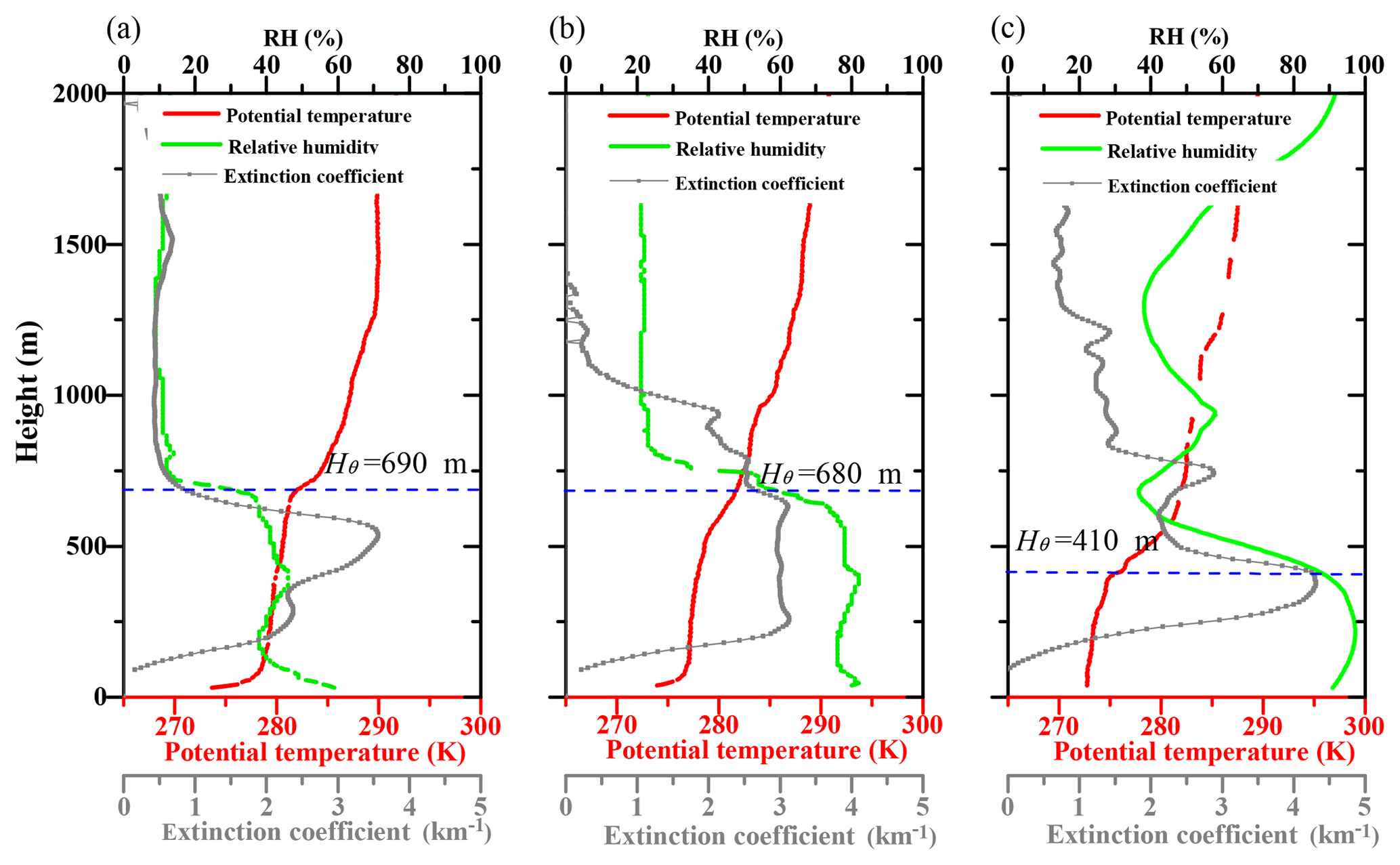
Figure 5 Vertical profiles measured from the ZBAA meteorological station: (a) 20:00, 16 December 2016; (b) 20:00, 17 December 2016; and (c) 08:00 21 December 2016. Red line: potential temperature (K); green line: RH (%); grey line: extinction coefficient (km⁻¹); dotted blue line: ABL height determined by radiosondes and expressed in H_θ (m).

3.3 Boundary layer structure observed by radiosonde technologies

Radiosonde instruments are the most widely used tools for conventional meteorological observation. The white points shown in Fig. 4 denote the ABL height determined from radiosonde data. The potential temperature (θ) determined by radiosonde technology is calculated from the following formula: $\mathit{\theta }=T+{\mathit{\gamma }}_{d}z$, γ_d=0.00975 K m⁻¹ (Stull, 1988); T is the measured temperature. As noted in many previous studies, the most widely used approach for the determination of the ABL height and structure for the daytime and nighttime involves identifying local maxima in potential temperature vertical gradient profiles as measured by radiosonde devices (Seibert et al., 2000; Summa et al., 2013; Sorbjan, 1989), but this method is only appropriate to apply to the convective ABL (Hennemuth and Lammert, 2006). Since the pollution period we examine involves stagnant winter weather conditions and as our radiosonde data only apply to dawn and dusk periods (08:00 and 20:00 LT), a stable boundary layer often appears (see Fig. 5, for example) and the height of the stable boundary layer (SBL) is more difficult to determine (Keller et al., 2010; de Jong et al., 2015; Schäfer et al., 2006). In this study, the level showing an obvious change in the potential temperature gradient and the profile of relative humidity were used to define the ABL height, as expressed by H_θ (see the blue dotted lines in Fig. 5). Under stagnant and heavily polluted weather conditions, turbulence is more heavily suppressed than under normal weather conditions, and the top of the residual layer can also characterize the thickness of the stable boundary layer to some extent. We can also use the minimum value of the relative humidity (green curves shown in Fig. 5) gradient to determine the height of the SBL. The atmospheric stratification of potential temperature and RH can affect the distribution of aerosol concentrations, which in turn affects the extinction coefficient. In Fig. 5, vertical profiles of the extinction coefficient observed by lidar during the same period are also given.

As shown in Fig. 5, the pollution episode was often accompanied by an inversion layer, as the vertical gradient of PT is positive, implying that the atmosphere was basically stable. The fact that the planetary boundary layer (PBL) was stable is unsurprising given the timing of radiosonde profiles at 08:00 and 20:00 local time (LT), which, respectively, occur approximately 30 min after sunrise and 3 h after sunset during the experimental period. Thus, a nocturnal inversion should barely be eroded by 08:00 LT (if at all, depending on the energy balance as insolation levels are low), and a nocturnal inversion should form by 20:00 LT. Due to this timing, these profiles are not representative of daytime conditions when pollutants are actively mixed. Midday profiles (noon local time or the early afternoon) would instead present instability and mixing. Air pollutants are generally blocked below the inversion layer and are not easily diffused to high levels. Figure 5a shows that H_θ at 20:00 LT on 16 December was approximately 690 m, where the potential temperature was approximately 280 K and the RH was approximately 20 %, and the extinction coefficient was also reduced to 0.7 km⁻¹. Due to the cooling effects of surface longwave radiation, the ground inversion layer formed from the surface at a depth of approximately 100 m. At this time, the potential temperature gradient underwent an obvious change at 600 m. The inversion intensity levels below 600 m were weaker, and the height H_θ was approximately 690 m. The most negative value of the extinction coefficient gradient appeared at approximately 500 m at this time, and the extinction coefficient below 690 m was much higher than that observed above 690 m, indicating that aerosol particles were mainly concentrated below the inversion layer (Baumbach and Vogt, 2003) and that the H_θ calculated by radiosondes is basically consistent with H_c determined by lidar.

At 20:00 LT on 17 December, ground inversion started to form. H_θ was observed at approximately 680 m, and the potential temperature at this level was still at approximately 280 K, though the RH reached nearly 60 %. Below this height, the whole atmosphere layer had developed a high-humidity layer with an RH of nearly 80 % from the ground, and the corresponding extinction coefficient had also increased significantly. The extinction coefficient between 250 and 600 m was almost 3 km⁻¹, revealing that the concentration of aerosols had increased significantly. Combined with the wind direction at this time (Fig. 6d), it is clearly observed that the transport of easterly winds moved considerable levels of water vapor from Bohai Bay (approximately 200 km east of Beijing), which promoted the hygroscopic growth of aerosol particles (Svenningsson et al., 1992; Chuang, 2003; Pan et al., 2009). At 08:00 LT on 21 December, the potential temperature distribution in the morning was different from that observed at 20:00 LT, and the surface temperature had begun to increase as solar radiation was received and the H_θ was approximately 410 m. The value below 300 m was nearly 95 %, while the maximum extinction coefficient, which exhibited bimodal features, reached nearly 4 km⁻¹. The altitude at which the extinction coefficient reached peak levels in the lower layer was approximately H_θ. By means of analyzing and comparing H_c and H_θ values, it is apparent that when concentrations of PM_2.5 were high, the accumulation of pollutants was mainly accompanied by the inversion layer in the atmosphere. The potential temperature gradient at the inversion layer is generally larger. Even though H_c reflects aerosol scattering information and H_θ denotes potential temperature characteristics, there is a strong correlation between them with a correlation coefficient of approximately 72 %. As shown in Fig. 4, H_θ was significantly higher than H_c determined by the three methods based on the lidar extinction coefficient.

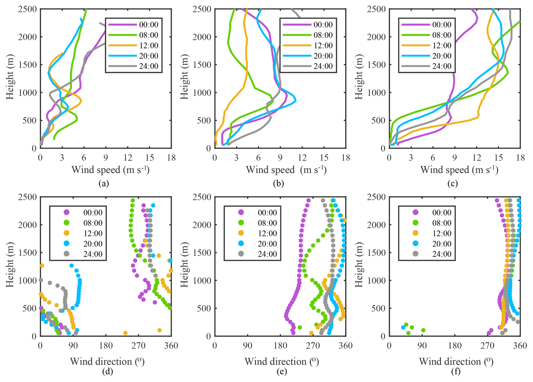
Figure 6 Vertical profiles of wind speed (m s⁻¹) and wind direction (^∘) observed by WPR. (a, d) 17 December 2016; (b, e) 21 December 2016; (c, f) 22 December 2016.

3.4 Boundary layer structure observed by WPR

The ground is the most important sink of atmospheric momentum, and the wind speed is zero at the Earth's surface. The ABL wind speed gradually changes from the Earth's surface to the geostrophic winds measured at high altitudes, and the wind information extracted from the WPR has been widely used to analyze wind characteristics. A comprehensive review of convective boundary layer heights is given by Seibert et al. (2000).

To analyze the influence of the boundary layer's wind structure on pollutants, we further discuss the representative wind speed and direction profiles of the three typical days for the unpolluted and polluted conditions. As is shown in Fig. 6, wind speeds below 1000 m did not exceed 6 m s⁻¹ on 17 December. At 12:00 LT a typical “nose” profile distribution formed according to the wind profile, with a maximum value observed in the middle of the wind profile. The wind direction profiles show that the wind direction from the ground to approximately 750 m was northeasterly (0–90^∘) and the wind direction observed above 750 m was northwesterly (270–360^∘). Furthermore, the wind directions from 750 to 2000 m remained basically stable in the northwesterly direction, echoing geostrophic winds. The height of low-level maximum wind corresponded to the height where wind direction changed into geostrophic wind. In addition to 12:00 LT on 17 December, at four other times almost strictly northeastern winds formed below 1000 m, and winds began to transform into the northwesterly winds at different heights. Wind speeds increased to some extent on 21 December with typical “nose” type wind speed distributions observed at 00:00, 08:00 and 20:00 LT. From the ground to 2500 m steady southwesterly winds formed at 00:00 LT, and the maximum wind speed was approximately 900 m. At this time, the extinction coefficient was also very low above 750 m (shown in Fig. 6), demonstrating that pollutants also formed below low-level maximum wind. At 12:00 LT the wind speed began to decrease slightly from the ground, and no obvious changes were observed beyond approximately 1100 m where wind speeds reached approximately 4 m s⁻¹. Except at 00:00 LT on 21 December when southwesterly winds prevailed from the ground to high altitudes, the wind directions shifted to the northwest, though these wind speeds were less strong below 500 m, and wind speed maximum values formed at a height of approximately 1000 m.

Wind directions observed on 22 December were northwesterly from the low layer to the high layer, but the distribution of wind velocity profiles differed from that of 21 December. Wind speeds were based on no significant maximum value area, and the maximum wind speed of 500 m approached close to 12 m s⁻¹. According to the extinction coefficient distribution (shown in Fig. 4), the PM_2.5 concentration was greatly reduced on this day. H_θ obtained by radiosondes were relatively similar at this time and far higher than H_c.

3.5 Boundary structure and turbulence quantities observed from the 325 m tower

Based on high-resolution gradient observations (15-layer mean and 7-layer turbulence measurements), we can analyze the relationship between PM_2.5 and low-level turbulence, average wind speed and temperature. As shown in Fig. 7, both turbulent kinetic energy (TKE) and friction velocity (u_*) at 140 and 280 m were inversely correlated with ground level PM_2.5 concentrations. TKE and u_* can be calculated as follows (Stull, 1988): $\text{TKE}=\frac{\mathrm{1}}{\mathrm{2}}\left(\stackrel{\mathrm{‾}}{{u^{\prime }}^{\mathrm{2}}}+\stackrel{\mathrm{‾}}{{v^{\prime }}^{\mathrm{2}}}+\stackrel{\mathrm{‾}}{{w^{\prime }}^{\mathrm{2}}}\right)$; $u_{*}={\left({\stackrel{\mathrm{‾}}{u^{\prime }{w}^{\prime }}}^{\mathrm{2}}+{\stackrel{\mathrm{‾}}{v^{\prime }{w}^{\prime }}}^{\mathrm{2}}\right)}^{\mathrm{1}/\mathrm{4}}$. The maximum TKE levels observed on unpolluted days (15 to 16 December) reached approximately 7 m² s⁻² at 140 m while the TKE levels measured on hazy days (17 to 21 December) decreased sharply to very low values. After the start of the period of heavy haze pollution, TKE levels remained relatively low, and the change in TKE was not as significant when concentrations of PM_2.5 increased from 200 to 400 µg m⁻³. On the other hand, the time series for u_* is slightly different from that of TKE. It seems that the inverse correlation between u_* and PM_2.5 is more obvious than that of TKE for the heavy pollution period. In fact, even during the period of heavy haze, a slight fluctuation (diurnal variation) in PM_2.5 concentrations can be observed, and the diurnal variation in u_* follows the opposite pattern to that of the PM_2.5 phase.

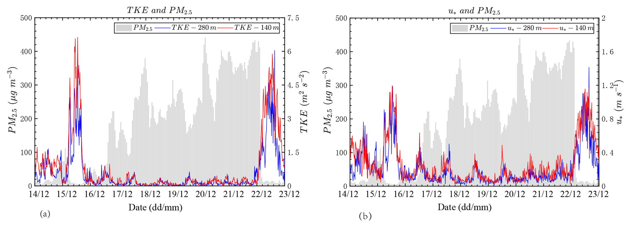
Figure 7 Time series of (a) turbulent kinetic energy (m² s⁻²) and (b) friction velocity (u_*, m s⁻¹) at 140 m (red line) and 280 m (green line); PM_2.5 (µg m⁻³) concentrations are also shown in the figures (grey columns).

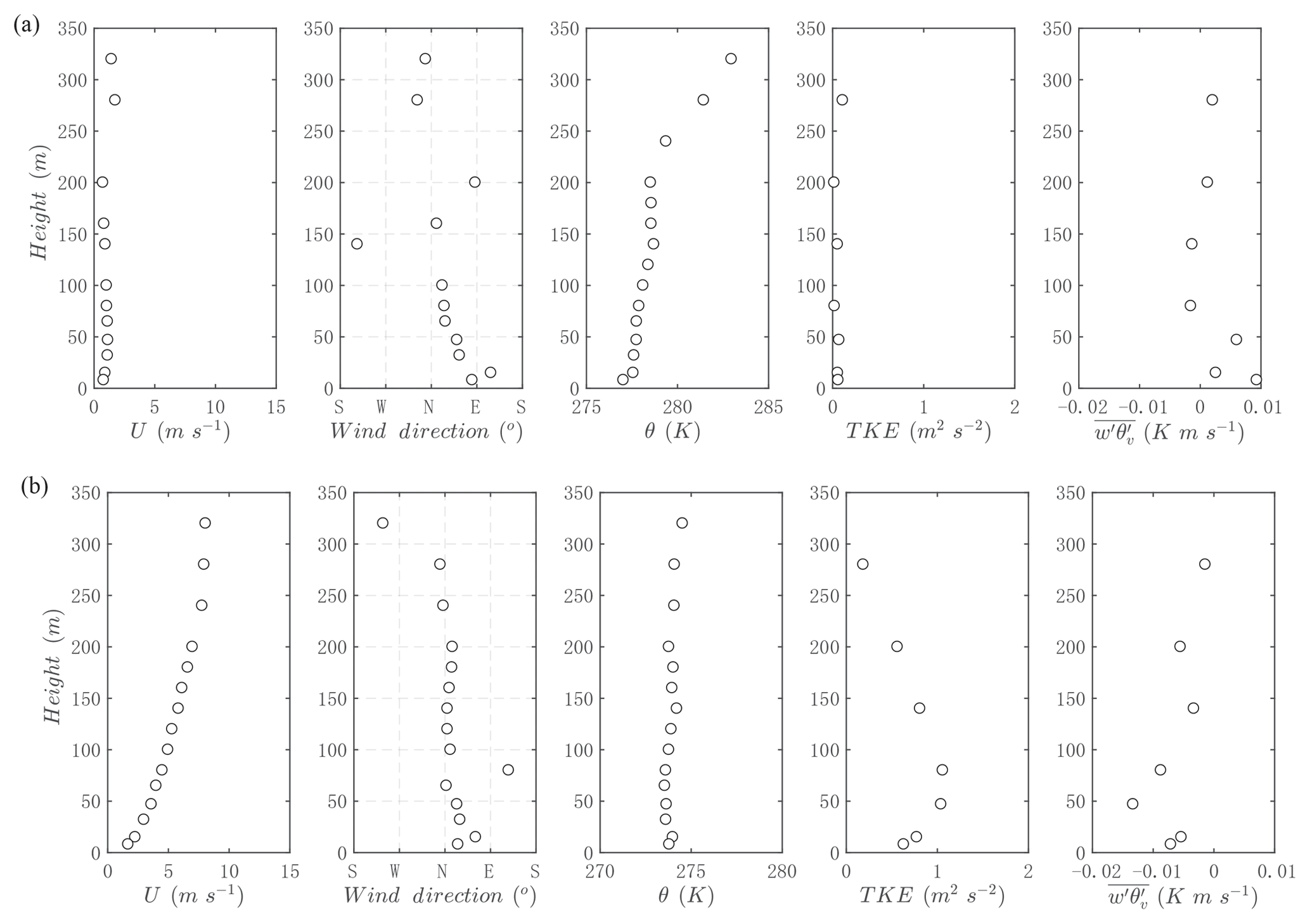
Figure 8 Vertical profiles of wind speed (U), wind direction (WD), potential temperature (θ), turbulent kinetic energy (TKE) and sensible heat flux ($\stackrel{\mathrm{‾}}{w^{\prime }{\mathit{\theta }}_{\mathrm{v}}^{\prime }}$) at 23:20 LT on 19 December 2016 (a), 22 December 2016 (b).

To understand the vertical structure characteristics of the ABL observed from the tower during the polluted and unpolluted periods, profiles for wind, potential temperature (θ), TKE and sensible heat flux ($\stackrel{\mathrm{‾}}{w^{\prime }{\mathit{\theta }}_{\mathrm{v}}^{\prime }}$) for the lower boundary layer are also given. At night (see Fig. 8), the wind speed profile for the clear day basically follows a logarithmic distribution and the potential temperature changes little from the ground to approximately 300 m. For turbulent values, TKE gradually decreased from approximately 70 m, and sensible heat flux was basically negative. On polluted days, wind speeds from the lower layer to the upper layer were valued at less than 2 m s⁻¹. At this time, the change in potential temperature was not very large from the ground to approximately 200 m, indicating that the atmosphere basically maintained neutral levels of stratification. A pronounced inversion layer cap is also observed to approximately 200 m from the surface. TKE levels were basically maintained at close to zero. Note that at this time the sensible heat flux measured at above 80 m remained at close to zero. Close to the ground, sensible heat flux was slightly positive, demonstrating that when pollution occurred and especially when the inversion layer existed, heat flux transport was suppressed. At night, surface longwave radiative cooling was restrained to a certain extent, and the weakening of turbulence activities aggravated pollution levels again.

In the daytime on 21 December 2016 (see Fig. 9), the PM_2.5 concentrations reached roughly 400 µg m⁻³, wind speeds were low, TKE remained at zero value and the potential temperature observed from the tower during the period of pollution basically denoted neutral stratification. The sensible heat flux was positive, but the value was basically measured as 0.02 K m s⁻¹. At noon on 22 December, when the weather had improved, wind speeds were clearly higher. TKE still reached a maximum at 47 m. The influence of the urban canopy was stronger at heights of below 47 m. Unlike on the polluted day, levels of sensible heat flux were higher at this time and the lower layer reached a value of 0.1 K m s⁻¹. The tower observation data clearly show that levels of sensible heat flux decreased significantly in the daytime during the haze episode because of the higher levels of solar radiation scattering by particles.

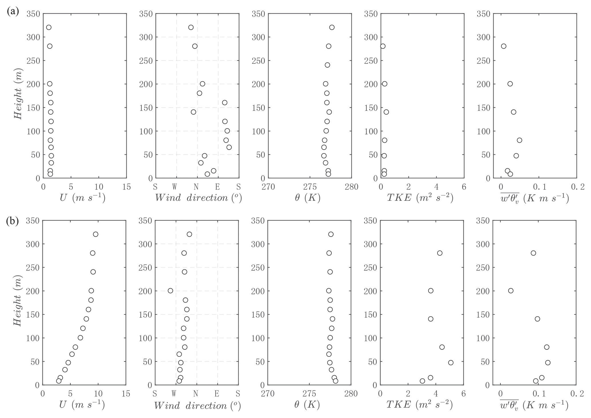
Figure 9 Vertical profiles of wind speed (U), wind direction (WD), potential temperature (θ), turbulent kinetic energy (TKE) and sensible heat flux ($\stackrel{\mathrm{‾}}{w^{\prime }{\mathit{\theta }}_{\mathrm{v}}^{\prime }}$) measured at 12:00 LT on 21 December 2016 (a) and 22 December 2016 (b).

Table 2 Averaged values of visibility (Vis), wind speed (U), relative humidity (RH), ABL height (H_c), turbulent kinetic energy (TKE), friction velocity (u_*), momentum flux ($\stackrel{\mathrm{‾}}{u^{\prime }{w}^{\prime }}$) and sensible heat flux ($\stackrel{\mathrm{‾}}{w^{\prime }{\mathit{\theta }}_{\mathrm{v}}^{\prime }}$) for different levels of pollution. Corresponding relationships between air pollution levels and PM_2.5 concentrations are as follows: good (0–75 µg m⁻³), slightly polluted (75–115 µg m⁻³), moderately polluted (115–150 µg m⁻³), heavily polluted (150–250 µg m⁻³) and seriously polluted (>250 µg m⁻³).

According to the concentration of PM_2.5 observed, the haze pollution episode can be divided into different grades. Statistical mean values of surface visibility (Vis), wind speed (U), RH, ABL heights and turbulent fluctuations are also calculated. As is shown in Table 2, the statistical averages further confirm the conclusions of the previous analysis. Instead, when the concentration of PM_2.5 is high, visibility and wind speed decrease while RH increases significantly. Our results show that due to the accumulation of aerosol particles, H_c is heightened slightly. The lidar results overestimate the ABL height at night (Quan et al., 2013). In this study the ABL height also increased due to the accumulation of pollutants during the period of heavy pollution. The turbulence levels observed also exhibit a decreasing trend occurring during the haze pollution episode, further demonstrating that turbulent activities are inhibited to a certain extent. We note that there appears to be only slight differences between the ABL height under slightly, moderately, heavily and seriously polluted conditions. Since the data examined in this study apply to only one period of heavy pollution, the minor differences observed may not be statistically different across categories except when compared to “good” air quality conditions.

4 Conclusions

In this paper a red-alert haze pollution period running from 14 to 22 December 2016 occurring in Beijing was studied using various observational techniques. Atmospheric boundary layer structures and turbulence characteristics are the focus of this paper. Observational techniques used include not only remote sensing techniques, e.g., lidar and WPR, but also direct measurement techniques, e.g., ground-based radiosonde technologies and the 325 m meteorological tower. Our research results show that during the studied period of heavy haze pollution, the Beijing area was controlled by a stagnant weather system and wind speed in the surface layer was small. Although there were weaker diurnal changes, the atmospheric boundary layer tended to be stable overall, until the late strong wind weather process arrived. Water vapor transport increased the relative humidity at levels below 600 m, greatly promoting the hygroscopic growth of PM_2.5. The ABL height observed by lidar (H_c) was about 500–750 m. The vertical distribution of pollutant concentration is highly correlated with the inversion layer.

With the development of the haze pollution process, the maximum nocturnal inversion height has been significantly reduced, and its lowest value was below 500 m. But H_c did not seem to decrease due to the accumulation of pollutants. Based on the potential temperature gradient method, the ABL height calculated by radiosonde data (H_θ) was in good agreement with H_c with a correlation coefficient close to 72 %. Turbulent kinetic energy TKE and friction velocity u_* measured at different heights on the tower had obvious inverse correlation with surface PM_2.5 concentration. Turbulence was very weak in the whole haze pollution period. Momentum and heat fluxes close to the Earth's surface always stay positive, indicating that the cooling effect of long-wave radiation from the ground is inhibited. In the daytime, turbulence was suppressed due to the solar radiation scattering by the high concentration of particulate matter, and sensible heat fluxes were greatly reduced within 300 m from the ground.

It seems that when heavy pollution occurs, the height (H_c) measured by lidar can better reflect the accumulation of pollutants than H_θ because lidar can continuously measure the extinction coefficient of fine particles. In principle, the boundary layer height measured by different observation methods should be different because the measurement principle of the instrument is different: some measure material properties (such as pollutants in the air) and others measure the physical properties of the atmosphere (such as temperature).

Our future work will further explore the relationship between the boundary layer heights measured by different means and will be meaningful by deeply exploring the correlations between H_θ and H_c through more observational and theoretical study. In addition, this future study will also be made meaningful by establishing a relationship between the parameterized friction velocity and the PM_2.5 concentration because these exhibit a strong statistical correlation (negative correlation) in numerical models of air pollution.