Ozone Monitoring Instrument (OMI) Total Column Water Vapor version 4 validation and applications

Total column water vapor (TCWV) is important for the weather and climate. TCWV is derived from the Ozone Monitoring Instrument (OMI) visible spectra using the version 4.0 retrieval algorithm developed at the Smithsonian Astrophysical Observatory. The algorithm uses a retrieval window between 432.0 and 466.5 nm and includes updates to reference spectra and water vapor profiles. The retrieval window optimization results from the trade-offs among competing factors.

The OMI product is characterized by comparing against commonly used reference datasets – global positioning system (GPS) network data over land and Special Sensor Microwave Imager/Sounder (SSMIS) data over the oceans. We examine how cloud fraction and cloud-top pressure affect the comparisons. The results lead us to recommend filtering OMI data with a cloud fraction less than f=0.05–0.25 and cloud-top pressure greater than 750 mb (or stricter), in addition to the data quality flag, fitting root mean square (RMS) and TCWV range check. Over land, for f=0.05, the overall mean of OMI–GPS is 0.32 mm with a standard deviation (σ) of 5.2 mm; the smallest bias occurs when TCWV = 10–20 mm, and the best regression line corresponds to f=0.25. Over the oceans, for f=0.05, the overall mean of OMI–SSMIS is 0.4 mm (1.1 mm) with σ=6.5 mm (6.8 mm) for January (July); the smallest bias occurs when TCWV = 20–30 mm, and the best regression line corresponds to f=0.15. For both land and the oceans, the difference between OMI and the reference datasets is relatively large when TCWV is less than 10 mm. The bias for the version 4.0 OMI TCWV is much smaller than that for version 3.0.

As test applications of the version 4.0 OMI TCWV over a range of spatial and temporal scales, we find prominent signals of the patterns associated with El Niño and La Niña, the high humidity associated with a corn sweat event, and the strong moisture band of an atmospheric river (AR). A data assimilation experiment demonstrates that the OMI data can help improve the Weather Research and Forecasting (WRF) model skill at simulating the structure and intensity of the AR and the precipitation at the AR landfall.

1 Introduction

Water vapor is of profound importance for weather and climate. Through condensation, it forms clouds that modify albedo, affect radiation and interact with particulate matter. In addition, latent heat released from water vapor condensation can influence the atmospheric energy budget and circulation. Water vapor is the most abundant greenhouse gas, accounting for ∼50 % of the greenhouse effect (Schmidt et al., 2010). Thus, monitoring the spatial and temporal distributions of water vapor is crucial for understanding water-vapor-related processes.

Water vapor has been measured using a variety of in situ and remote sensing techniques from the ground, air and space. Satellite data provide a global perspective and are indispensable for constraining reanalysis products (Dee et al., 2011; Gelaro et al., 2017). The current satellite water vapor datasets are evaluated through the Global Energy and Water cycle Exchanges (GEWEX) Water Vapor Assessment program (Schröder et al., 2019). These datasets are derived from visible, near-infrared (NIR), infrared (IR), microwave and global positioning system (GPS) measurements. Each dataset has its own characteristics and contributes to the understanding of water vapor in its own way. For example, microwave data are useful for both clear-sky and cloudy-sky conditions but are best suited for nonprecipitating ice-free oceans due to the complications associated with land-surface emissivity; NIR data are best suited for the land, as the surface albedo is low over the oceans; IR data are available over all surface types but are strongly influenced by clouds and less sensitive to the planetary boundary layer; visible data are sensitive to the boundary layer over both land and the oceans but are complicated by uncertainties in clouds and aerosols (Wagner et al., 2013).

Total column water vapor (TCWV, also called integrated water vapor – IWV – or precipitable water vapor – PWV) can be retrieved from the 7ν water vapor vibrational polyad band (around 442 nm) despite the weak absorption (Wagner et al., 2013). This made it possible to derive TCWV from instruments measuring in the blue wavelength range. Since water vapor is a weak absorber here, saturation of spectral lines is not of concern (Noël et al., 1999). Moreover, the similarity between the land and ocean surface albedo in the blue wavelength range suggests a roughly uniform sensitivity of the measurement over the globe (Wagner et al., 2013). However, weaker absorption tends to result in larger relative uncertainties, especially for a low TCWV amount.

Using the visible spectra measured by the Ozone Monitoring Instrument (OMI), Wang et al. (2014) retrieved version 1.0 TCWV from 430–480 nm and publicly released the data on the Aura Validation Data Center (AVDC; https://avdc.gsfc.nasa.gov, last access: 17 September 2019). Wang et al. (2016) found that the version 1.0 data generally agree with ground-based GPS data over land but are significantly lower than the microwave observations over the oceans. They found that using a narrower retrieval window (427.7–465 nm) in version 2.1 could improve the data over the oceans without adversely affecting the results over land much. However, the version 2.1 data were only generated for a few test months and not released to the public. An interim version 3.0 OMI TCWV product was available at the AVDC. Compared with version 2.1, version 3.0 uses the reference spectrum for water vapor from the latest HITRAN database (Gordon et al., 2017) and that for liquid water from Mason et al. (2016), as well as the newest cloud product (Veefkind et al., 2016). The version 3.0 retrieval window (427.0–467.0 nm) is adjusted from that for version 2 within 2 nm on each end based on fitting uncertainty for a randomly selected test orbit.

This paper focuses on version 4.0 OMI TCWV, which has replaced version 3.0 at the AVDC. We present the version 4.0 retrieval algorithm, which incorporates a more vigorous systematic optimization for the retrieval window and miscellaneous updates. We characterize the performance of the version 4.0 dataset by comparing with well-established references, such as the GPS network data and Special Sensor Microwave Imager/Sounder (SSMIS) observations. We also assess the performance of version 4.0 against that of version 3.0. To provide a practical guide to users of the new data, we investigate the influence of cloud fraction and cloud-top pressure on the comparisons. Based on the results, data filtering criteria are recommended. As an additional check on the version 4.0 product, we show test applications of the data to a range of spatial and temporal scales, including El Niño–La Niña, a corn sweat event and an atmospheric river (AR) event. For the first time, a data assimilation experiment for the AR event demonstrates that the OMI TCWV data can provide a useful constraint for weather prediction.

2 Retrieval algorithm

OMI, onboard the Aura spacecraft, is a UV–visible imaging spectrometer (Levelt et al., 2006). It has been making daily global observations at a nominal 13×24 km nadir resolution from a 13:30 Equator crossing local time polar orbit since October 2004. The UV–visible channel of OMI covers 350–500 nm at a spectral resolution of about 0.5 nm.

TCWV is derived from the OMI visible spectrum using a two-step approach. First, the slant column density (SCD; molecules cm⁻²) is retrieved from a spectral fitting algorithm. Then, the vertical column density (VCD; molecules cm⁻²) is calculated from the ratio of SCD and air mass factor (AMF) (Palmer et al., 2001). VCD can be converted to TCWV using 10²³ molecules cm${}^{-\mathrm{2}}=\mathrm{29.89}$ mm. The details of the two-step procedure can be found in González Abad et al. (2015). The specifics of version 4.0 are discussed below.

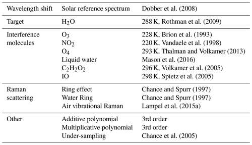
The version 4.0 spectral fitting parameters are summarized in Table 1. In the nonlinear least-squares fitting, we consider wavelength shift, under-sampling, closure polynomials (3rd-order multiplicative and additive), reference spectroscopic spectra of water vapor, interfering molecules (O₃, NO₂, O₄, liquid water, C₂H₂O₂ and IO) and Raman scattering (the Ring effect, vibrational Raman scattering of air and the water Ring effect). In comparison with previous versions, version 4.0 no longer fits the common mode (i.e., the mean of the fitting residual; González Abad et al., 2015). It turns out that the common mode for land is different than that for ocean (Wang et al., 2014). Previous retrievals derive a common mode for each orbit swath using the pixels in the low latitudes, which often includes both land and ocean scenes. Thus, the derived common mode depends on the proportion of land versus ocean pixels of the spacecraft orbit and is not universally suitable for all the pixels of the swath. Statistics for Orbit 10 423 show that although the mean SCD differs little between the retrievals with and without the common mode in the fitting (0.1 mm), the standard deviation of SCD between them can be significant (1.7 mm). Most of the settings in Table 1 are shared between versions 3.0 and 4.0, except that version 3.0 uses HITRAN 2016 (Gordon et al., 2017) as the water vapor reference spectrum and includes a common mode in the fitting but does not consider the vibrational Raman scattering of air (Lampel et al., 2015a). We revert to the HITRAN 2008 water vapor spectrum (Rothman et al., 2009) in version 4.0 because validation results show that it leads to better agreement with the GPS and SSMIS TCWV data (Sect. 3). We did not apply the correction of Lampel et al. (2015b) to the HITRAN 2008 water vapor spectrum. It was recently found that HITRAN 2016 is adversely affected by an issue with line broadening for water vapor in the blue wavelength range, and improvements are being made for the next HITRAN release (the HITRAN group, personal communication, 28 June 2019).

Table 1 Parameters used in the version 4.0 spectral fitting for OMI total column water vapor.

To optimize the retrieval window, we randomly selected OMI Orbit 10 426 (on 1 July 2006) to examine the effect of varying the starting and ending wavelengths around the 7ν water vapor absorption band. The orbit swath contains 60×1644 ground pixels and covers parts of Australia, the Pacific, China and other areas. We systematically adjust the starting wavelength within 426.0–435.0 nm and the ending wavelength within 460.0–468.5 nm, both at 0.5 nm steps.

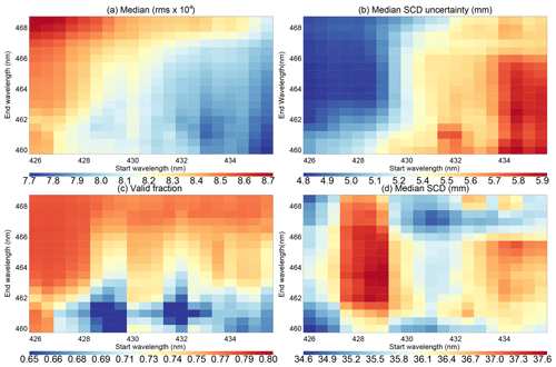
Figure 1 Sensitivity of the retrieval to the start and end wavelengths (nm) of the retrieval window for OMI Orbit 10 426. (a) Median of fitting RMS × 10⁴; (b) median of water vapor SCD fitting uncertainty in millimeters; (c) valid fraction for retrievals; (d) median SCD in millimeters.

In previous versions, the fitting window is selected based on the fitting uncertainty (Wang et al., 2014, 2016). For version 4.0, we consider the following four factors. (1) Figure 1a shows that the median of the fitting root mean square error (RMS) is smaller toward the lower right corner of the domain (i.e., longer start wavelength and shorter end wavelength). (2) Figure 1b shows that the medium fitting uncertainty of water vapor SCD decreases toward the upper left corner. (3) Figure 1c shows that the fraction of valid retrievals for the orbit generally increases toward the upper part of the domain. Valid retrievals here refer to those that pass the main data quality check (MDQFL = 0) and have positive SCDs. The main data quality check ensures that the fitting has converged and that the SCD is $<\mathrm{5}\times {\mathrm{10}}^{\mathrm{23}}$ molecules cm⁻² (149.45 mm) and within 2σ of the fitting uncertainty. The SCD threshold here is meant to filter out large outliers. For reference, the largest TCWV of the GPS and SSMIS datasets used in Sect. 3 is about 75 mm. At low latitudes at which TCWV is large, more than 90 % of the OMI AMFs are between 0.5 and 2.0. (4) The length of the retrieval window increases with the difference between the end and start wavelengths. The general patterns exhibited by Orbit 10 426 in Fig. 1 also hold for Orbit 10 423, which cuts across the Pacific near the dateline.

Ideally, we would like to have a small fitting RMS to reduce the residual's amplitude and structure, a small fitting uncertainty to reduce error, a large fraction of valid data to increase data volume and a long retrieval window to include more information into the fitting. However, these criteria cannot be met simultaneously. As a compromise, we select the wavelength interval between 432.0 and 466.5 nm as the retrieval window for version 4.0. For Orbit 10 426, this leads to a median fitting RMS of $\mathrm{8.1}\times {\mathrm{10}}^{-\mathrm{4}}$, a median SCD uncertainty of 5.4 mm, a valid fraction of 0.75 and a window length of 34.5 nm (Fig. 1). Figure 1d shows that the median SCD for Orbit 10 426 varies between 34.6 and 37.6 mm. This 3 mm difference corresponds to an 8 % variation and exhibits a complex pattern within the domain. The version 4.0 retrieval window leads to a median SCD of 35.5 mm for Orbit 10 426, which is near the beginning of the middle third of the SCD range. The ratio between the median SCD uncertainty and the median SCD (i.e., the relative SCD uncertainty) is about 0.15. Note that this value is for the whole orbit, which includes a wide range of SCDs. As shown in Fig. S1 in the Supplement, the relative SCD uncertainty is >1.2 for SCD = 0–10 mm; it drops to about 0.4 for SCD = 10–20 mm and to about 0.1 for SCD >40 mm.

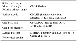
The AMF is calculated by convolving scattering weights with the shape of the water vapor vertical profile (González Abad et al., 2015). The scattering weight is interpolated from the same lookup table as that used in Wang et al. (2016). The scene-specific information used in the AMF calculation is listed in Table 2. By propagating typical errors for surface albedo (15 %), cloud fraction (10 %) and cloud-top pressure (15 %), we find that the AMF error due to scattering weight for a typical orbit (Orbit 10 426) is mostly <3 %, though for cloudy pixels, the error can be 15 % or more. Version 4.0 uses the ${\mathrm{0.5}}^{\circ }\times {\mathrm{0.667}}^{\circ }$ monthly mean MERRA-2 water vapor profile (Gelaro et al., 2017) for the month and year corresponding to the retrieval, while previous versions used the monthly mean of 2007 for all years. To evaluate the error associated with gas profiles, we compare the TCWV calculated using the daily MERRA-2 profile against that calculated using the monthly MERRA-2 profile for July 2006 (for TCWV within the 0–75 mm range). Results show that (TCWV(daily)–TCWV(monthly)) has a mean (median) of 0.3 mm (0 mm) with a standard deviation of 5.0 mm. When comparing the TCWV calculated using the daily MERRA-2 profile against that calculated using the daily ERA-Interim profile for July 2006, we find that (TCWV(MERRA-2)–TCWV(ERA-Interim)) has a mean (median) of −0.1 mm (0 mm) with a standard deviation of 2.8 mm. Thus, gas profiles can introduce substantial scatter to the retrieved TCWV. AMF is highly sensitive to clouds (Wang et al., 2014; Vasilkov et al., 2017). Version 4.0 uses the cloud information from Veefkind et al. (2016). The primary difference with the Acarreta et al. (2004) cloud product used in versions 1.0 and 2.1 is the cloud-top pressure for cloud fraction f<0.3. In addition to the factors in Table 2, the aerosol and surface bidirectional reflectance distribution functions (BRDFs) influence the AMF (Lorente et al., 2017; Vasilkov et al., 2017) but have not been considered in the retrieval yet.

Table 2 Parameters used in AMF calculation.

3 Validation

To validate the version 4.0 OMI TCWV data, we compare them against two commonly used reference datasets – a GPS network dataset for land and a microwave dataset for the oceans.

3.1 OMI and GPS over land

To assess the version 4.0 OMI TCWV over land, we compare against the GPS network data downloaded from NCAR (Wang et al., 2007) (https://rda.ucar.edu/datasets/ds721.1/, last access: 17 September 2019). The GPS data are composed of 2-hourly TCWV at International GNSS Service (IGS), SuomiNet and GEONET stations, and they have an estimated error of <1.5 mm (Wang et al., 2007; Ning et al., 2016). The subset of IGS–SuomiNet data for the whole year of 2006 is used in this paper. The geographical distribution of the stations can be found in Wang et al. (2016). Most of the stations are concentrated in North America and Europe, and a few are scattered on other continents.

OMI TCWV data are filtered using the following criteria. The stripes in Level 2 swaths due to systematic instrument error are removed using the SCD scaling procedure described in Wang et al. (2016). The pixels affected by OMI's row anomaly are filtered out (http://projects.knmi.nl/omi/research/product/rowanomaly-background.php, last access: 17 September 2019), as are negative or extremely large (i.e., TCWV > 75 mm) values. For the clear-sky comparison in Fig. 3, we require cloud fraction <5 % and cloud-top pressure >750 mb, in addition to MDQFL = 0 and fitting RMS < 0.001. The cloud fraction and cloud-top pressure are from the OMCLDO2 cloud product (Veefkind et al., 2016) and are included in the Level 2 OMI product for ease of data filtering. On a typical day (1 July 2006), among the OMI data that pass the MDQFL and TCWV range test, cloud fraction <0.05 accounts for 35 % of the data, cloud-top pressure >750 mb accounts for 53 % of the data and RMS <0.001 accounts for 72 % of the data.

To colocate GPS and OMI data, we select the GPS data observed between 12:00 and 15:00 LT. This 3 h local time range covers the OMI overpass time. We average the qualified OMI data within 0.25^∘ longitude × 0.25^∘ latitude of the GPS stations for each day. To minimize the influence of local topography (e.g., mountain peaks, river valleys), if a station's elevation is more than 250 m different than the mean elevation within the corresponding $\mathrm{0.25}{}^{\circ }\times \mathrm{0.25}{}^{\circ }$ grid square, then it is excluded from the analysis. The $\mathrm{0.25}{}^{\circ }\times \mathrm{0.25}{}^{\circ }$ topography was downloaded from http://www.temis.nl/data/topo/dem2grid.html. The comparison between OMI and GPS is made for TCWV within the range of 0–75 mm as the largest TCWV for the GPS data is about 75 mm. The colocating procedure leads to about 11 000 colocated data points for the entire year of 2006.

Figure 2 shows the comparison between the resulting colocated GPS and version 4 OMI TCWV. Figure 2a shows the histogram of OMI–GPS (in 0.5 mm bins). The bin from −0.5 to 0.0 mm corresponds to the peak of the distribution. The overall mean (median) of OMI–GPS is 0.32 mm (0.35 mm), with a standard deviation of 5.2 mm. The mean (median) absolute error is 3.9 mm (3.0 mm).

Figure 2b shows the joint distribution of the colocated GPS and version 4.0 OMI data. The count for each 0.5 mm bin is normalized by the maximum of all bins. About 34 % of the data have TCWV < 10 mm, 72 % have TCWV < 20 mm and 90 % have TCWV < 30 mm. There is a general linear correlation between GPS and OMI data, with a correlation coefficient of r=0.87 (R²=0.76). The linear regression line (OMI = 2.22 + 0.88 × GPS, where OMI and GPS TCWV are in millimeters) has a significant positive intercept and a slope that is less than one. This indicates a positive bias of OMI against GPS for small TCWV and a negative bias for large TCWV. Indeed, as indicated at the top of the panel, the mean of OMI–GPS for each 10 mm GPS TCWV bin decreases from 1.7 mm for TCWV = 0–10 to −2.3 mm for TCWV = 40–50 mm, though the fraction of data for TCWV > 40 mm is <3 %. The corresponding standard deviation (σ) increases from 3.5 to 7.9 mm. The minimum bias of 0.2 mm occurs for TCWV in the 10–20 mm bin. The large positive bias of the 0–10 mm bin (compared with the TCWV of the bin) has a significant adverse effect on the regression line. For TCWV > 10 mm, the regression line (OMI = 1.51 + 0.91 × GPS) is better.

In comparison, although version 3.0 OMI is similarly correlated with GPS (correlation coefficient r=0.86), it has a much larger positive bias of 2.8 mm (with a standard deviation of 5.5 mm). The large bias is attributed to the much larger SCD of version 3.0 (Fig. S2b), as the AMFs of both versions roughly follow the 1:1 line (Fig. S2a). Sensitivity tests show that the larger version 3.0 SCD is primary due to the water vapor reference spectrum. If the water vapor reference spectrum in version 4.0 is replaced with that of version 3.0 (Test 1), then the median SCD increases by about 4.5 mm for Orbit 10 423 (Fig. S2c). Modifying the retrieval window for version 3.0 cannot sufficiently reduce the retrieved SCD and therefore cannot create significantly better agreement with the reference TCWV data. As version 4.0 shows a better performance, this paper focuses on characterizing version 4.0 to provide useful information to potential users. In subsequent discussions, OMI data refer to version 4.0 unless specified otherwise.

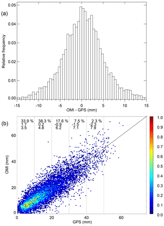
Figure 2 Comparison between colocated GPS and OMI TCWV (mm) for all days in 2006. The data filtering criteria include cloud fraction <5 %, cloud-top pressure >750 mb and others discussed in the text. (a) Relative frequency of occurrence for OMI–GPS (mm). (b) Normalized joint distribution of GPS versus OMI TCWV (mm). The three lines of text from top to bottom indicate the percentage of data points (first), the mean of OMI–GPS in millimeters (second) and the standard deviation of OMI–GPS in millimeters (third) for each 10 mm GPS TCWV, respectively. The 1:1 line is plotted for reference.

OMI TCWV retrieval is highly sensitive to clouds (Wang et al., 2014). In Fig. 3, we examine the effect of OMI cloud fraction threshold (f) on the comparison while keeping other data filtering criteria the same as those for Fig. 2 (i.e., cloud fraction <f, cloud-top pressure >750 mb, MDQFL = 0, fitting RMS <0.001 and 0 < TCWV < 75 mm). From f=0.05 to f=0.55, the number of colocated data pairs (N) more than triples, the mean of OMI–GPS increases from 0.32 to 1.66 mm and the standard deviation of OMI–GPS increases from 5.2 to 6.1 mm. The linear correlation coefficient (r) increases from r=0.87 at f=0.05 to r∼0.90 at f=0.15, then levels off for larger cloud fraction thresholds. It should be noted that the error in cloud-top pressure decreases with cloud fraction in the OMCLDO2 product (Veefkind et al., 2016). As a result, f=0.05 corresponds to the largest uncertainty in cloud-top pressure, and the error will propagate into OMI TCWV through AMF, leading to a smaller correlation coefficient than those for larger f values.

In addition, as shown by the GPS versus OMI joint distributions for different cloud fraction thresholds in Fig. 4, the f≥0.15 cases have larger effective dynamical ranges, which tend to favor better correlations. For example, there is a larger fraction of data pairs with TCWV >30 mm for f=0.15 than for f=0.05. The regression line for f=0.15 (OMI = 1.26 + 0.96 × GPS) shows an apparent improvement over that for f=0.05 (OMI = 2.22 + 0.88 × GPS). The best regression line is arguably that for f=0.25 (OMI = 1.16 + 0.99 × GPS) or f=0.35 (OMI = 1.19 + 1.00 × GPS), though the mean bias and scatter are larger than those for f<0.25 (Fig. 4).

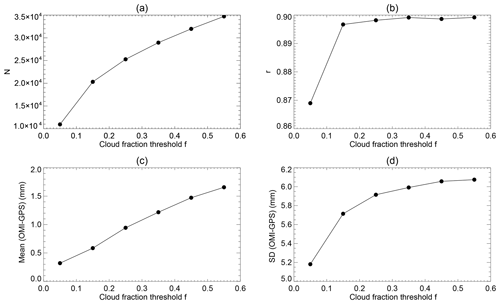
Figure 3 Dependence of various parameters on the cloud fraction threshold (f) used for filtering OMI data. Other filtering criteria remain the same as those for Fig. 2. The parameters are (a) the number of colocated OMI and GPS data pairs; (b) the linear correlation coefficient between OMI and GPS TCWV; (c) the mean of OMI–GPS in millimeters; and (d) the standard deviation of OMI–GPS in millimeters. Results are derived from the colocated version 4.0 OMI and GPS data for the whole year of 2006.

In brief, f=0.05 leads to the lowest overall bias and scatter of the colocated data; f=0.15 doubles the number of colocated data pairs and leads to the largest improvement in the correlation coefficient; f=0.25 (or 0.35) leads to the best linear regression line; the bias and standard deviation increase with cloud fraction threshold. Hence, cloud fraction thresholds in the range of f=0.05–0.25 seem reasonable for filtering OMI TCWV, depending on applications.

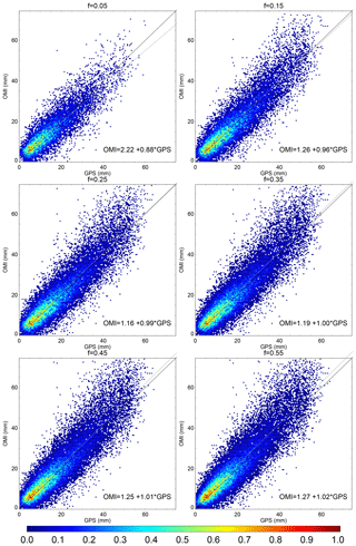
Figure 4 Normalized joint distributions of GPS versus version 4.0 OMI TCWV for different cloud fraction thresholds. Results are derived from the colocated data pairs for 2006. The OMI data filtering criteria are the same as those for Fig. 3. In each panel, the 1:1 line is plotted in black, and the linear regression line is plotted in gray and indicated by the formula in the lower right corner.

To further characterize the effect of cloud fraction threshold on the comparison between GPS and OMI, in Fig. 5 we examine the mean and standard deviation (σ) of OMI–GPS for each 10 mm GPS TCWV bin. The results are derived from the same sets of colocated GPS and OMI data as those used in Figs. 3 and 4. The filled symbols are for the cases in which the number of GPS and OMI data pairs within the corresponding TCWV bin is >1 % of the total number of data pairs, and the open symbols are for <1 %. As the filled symbols represent better statistics, we will focus on them below.

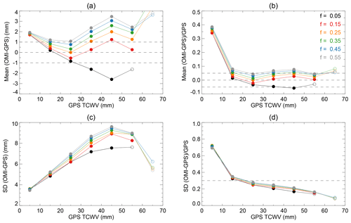
Figure 5 Parameters for each 10 mm TCWV bin. Curves with different colors are for different cloud fraction thresholds f as indicated in (b). The OMI filtering criteria remain the same as those for Figs. 3 and 4. Symbols are filled if the fraction of data pairs within the TCWV interval is >1 % of all the available data pairs and are open otherwise. The parameters are (a) mean OMI–GPS in millimeters, (b) relative bias defined as mean (OMI–GPS) ∕ GPS, (c) the standard deviation (σ) of OMI–GPS in millimeters and (d) relative scatter defined as σ ∕ GPS. Results are for all days in 2006. Dashed lines are meant to facilitate visualization.

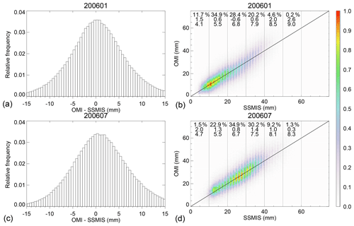
Figure 6 Comparisons between version 4.0 OMI and SSMIS over the oceans for (a, b) January 2006 and (c, d) July 2006. (a) The relative occurrence frequency of OMI–SSMIS (mm). (b) The normalized joint distribution of SSMIS versus OMI TCWV (mm).

Figure 5a shows that the means of OMI–GPS vary ±4 mm, following “V-shaped” curves whose minima occur in the TCWV = 20–30 mm bin except for f=0.05. The curves shift upward with increasing cloud fraction thresholds, suggesting that OMI cloudy-sky TCWV is generally larger than OMI clear-sky TCWV. Other things being equal, cloud formation indicates water vapor saturation and therefore a larger amount of TCWV than under clear-sky conditions. The smallest absolute bias for 10 < TCWV < 20 mm occurs at f=0.05, that for 20 < TCWV < 30 mm occurs at f=0.25 and that for 30 < TCWV < 40 mm occurs at f=0.15. The f=0.15 and f=0.25 curves show the best overall performance according to Fig. 5a as they are within 1 mm of zero for 10 < TCWV < 40 mm, while other curves come within 1 mm of zero in narrower TCWV ranges. Figure 5b shows the relative bias, which is defined as the mean of (OMI–GPS) ∕ GPS. The relative biases decrease sharply from ∼40 % to ∼5 %, as GPS TCWV increases from the TCWV = 0–10 mm bin to the TCWV = 10–20 mm bin, and generally stay less than ∼5–10 % for larger TCWV values. Figure 5c shows that σ increases from ∼3.5 mm for TCWV = 0–10 mm to ∼9.5 mm for TCWV = 40–50 mm (the percentage of data with TCWV > 50 mm is very small). In most cases, larger cloud fraction thresholds correspond to larger σ values. This is consistent with the larger dynamical range (due to a larger fraction of data with high TCWV) for a larger cloud fraction threshold (Fig. 4). In fact, the relative scatter, defined as the mean of σ ∕ TCWV, shows little difference among the f values (Fig. 5d). The relative scatter decreases with TCWV, with the sharpest decrease from ∼0.7 to ∼0.3 between TCWV = 0–10 mm and TCWV = 10–20 mm (Fig. 5d). The relative scatter continues to decrease for larger TCWV and the overall scatter is about 20 %.

In short, version 4.0 OMI agrees with GPS within 1 mm for 10 < TCWV < 40 mm when f=0.15 and f=0.25 are used; when f=0.05 is used, the bias and scatter are the smallest for 10 < TCWV < 20 mm; but, for TCWV < 10 mm, OMI TCWV is too high and has large relative scatter. The latter is expected from the low signal-to-noise ratio when TCWV < 10 mm in the OMI retrieval.

3.2 OMI and SSMIS over ocean

To evaluate version 4.0 OMI TCWV over the oceans, we compare against the microwave TCWV data from SSMIS onboard the Defense Meteorological Satellite Program (DMSP) F16 satellite. The SSMIS data are derived by Remote Sensing Systems (RSS) using their version 7 algorithm (http://www.remss.com/, last access: 17 September 2019) and have a retrieval accuracy of better than 1 mm (Wentz, 1997; Mears et al., 2015). For clear-sky comparison, we use the daily $\mathrm{0.25}{}^{\circ }\times \mathrm{0.25}{}^{\circ }$ SSMIS data for January and July 2006 and filter out the pixels affected by rain and cloud liquid water. Diedrich et al. (2016) found that the diurnal cycle in TCWV is generally within 1 % to 5 % of the daily mean, with a minimum between 06:00 and 10:00 LT and a maximum between 16:00 and 20:00 LT. To reduce the influence of the diurnal cycle, we average the SSMIS data for the ascending and descending orbits of F16 (∼20:00 and 08:00 LT in 2006).

We generate daily $\mathrm{0.25}{}^{\circ }\times \mathrm{0.25}{}^{\circ }$ Level 3 OMI TCWV from the de-striped Level 2 OMI swaths, with the requirement that MDQFL = 0, fitting RMS < 0.001, 0 < TCWV < 75 mm, cloud fraction <0.05 and cloud-top pressure >750 mb. There are typically 15 Level 2 swaths per day. The gridding program uses a tessellation method that weighs the contribution of a Level 2 data point by its area within the Level 3 grid square and its spectrum fitting uncertainty (Wang et al., 2014, 2016). The filtered daily Level 3 SSMIS and OMI data are compared for each month. We find 548 223 and 847 678 colocated data pairs for January and July 2006, respectively.

Figure 6a and c show the distribution of OMI–SSMIS for January and July 2006. For July, the mean of OMI–SSMIS is 1.1 mm with a standard deviation of 6.8 mm, and the mean absolute error of OMI–SSMIS is 5.2 mm. For January, the mean error, standard deviation and mean absolute error are 0.4, 6.5 and 5.0 mm, respectively. This suggests a slightly better agreement for January than for July. In comparison with the OMI–GPS over land (Sect. 3.1), OMI–SSMIS over the oceans has a somewhat larger bias and standard deviation. However, as TCWV over the oceans is generally larger than that over land (compare Figs. 6 and 2), the relative bias and scatter are actually similar.

Figure 6b and d show the normalized joint distribution of SSMIS versus OMI for January and July 2006. The correlation coefficients are r=0.84 and 0.82 for January and July, respectively. For January, OMI–SSMIS remains within 0.6 mm of zero for TCWV in the 10–40 mm range but is 1.5 mm for TCWV in the 0–10 mm range (only a small fraction of data pairs have TCWV > 40 mm). For July, OMI–GPS is 0.8 mm for the TCWV = 20–30 mm bin and varies between 0.8 and 1.4 mm for TCWV in the 10–50 mm range (only a small fraction of data pairs have TCWV < 10 mm or >50 mm). For TCWV bins that have >5 % of the data pairs, the standard deviation of OMI–SSMIS varies between 4.1 and 8.1 mm. Overall, version 4.0 OMI data compare reasonably well with SSMIS data for TCWV in the 10–40 mm range, with the smallest bias occurring in the TCWV = 20–30 mm bin.

The agreement between version 4.0 OMI with SSMIS is better than that between version 3.0 OMI and SSMIS. For July 2006, using the same data filtering criteria as before, we find that version 3.0 OMI–SSMIS has a mean of 3.2 mm with a standard deviation of 7.8 mm. The bias is much larger than that for version 4.0 OMI–SSMIS. Again, this is because of the much larger SCD of version 3.0 OMI TCWV due to the water vapor reference spectrum (Fig. S1).

Table 3 shows the effect of cloud fraction threshold (f) on the comparison between SSMIS and version 4.0 OMI TCWV. The comparisons are performed using daily filtered Level 3 data for July 2006. For SSMIS, we only filter out pixels affected by rain. To investigate the influence of clouds, cloud liquid water is not used to filter the SSMIS data here. This is less restrictive than the criteria used for Fig. 6 as the SSMIS pixels with cloud liquid water are filtered out in Fig. 6 for the “clear-sky” comparison there. For OMI, we require MDQFL = 0, RMS < 0.001, 0 < TCWV < 75 mm, cloud-top pressure > 750 mb and cloud fraction <f. Results show that OMI is higher than SSMIS by 0.02–3.07 mm for f=0.05–0.45. The difference between the f=0.05 case in Table 3 and the f=0.05 case in Fig. 6 is due to the relaxed SSMIS filtering criteria. The closest agreement in terms of the mean and standard deviation of OMI–SSMIS occurs when f=0.05. The number of SSMIS and OMI data pairs more than doubles between f=0.05 and f=0.15. The linear correlation coefficient varies between 0.82 and 0.85 within the range of f values considered. The best linear regression line (OMI = 0.70 + 1.02 × SSMIS) occurs when f=0.15. Therefore, for OMI over the oceans, we recommend using cloud fraction threshold f=0.05–0.15 in combination with the other usual data filtering criteria, though users are advised to make their own decisions based on their tolerance and applications.

Table 3 Effect of cloud fraction threshold on the comparison between SSMIS and version 4.0 OMI TCWV for July 2006.

f: OMI cloud fraction threshold; N: number of qualifying data pairs; P: percentage of qualifying data pairs with respect to the total number of qualifying SSMIS data points; Mean: mean of OMI–SSMIS in millimeters; σ: standard deviation of OMI–SSMIS in millimeters; MAE: mean absolute error OMI–SSMIS in millimeters; r: correlation coefficient between SSMIS and OMI; R²: coefficient of determination for linear regression OMI = b + k × SSMIS, where OMI and SSMIS are in millimeters; b: intercept of linear regression; k: slope of linear regression.

Lowering the value for the cloud-top pressure threshold also leads to larger bias and scatter. For example, when cloud fraction threshold f=0.05 and cloud-top pressure >500 mb are used, the mean and standard deviation of OMI–SSMIS become 0.80 and 7.9 mm; both are larger than those for f=0.05 in Table 3, though the linear regression line improves to OMI = 0.63 + 1.01 × RSS due to an increase in the dynamical range of TCWV. It should be noted that the OMCLDO2 cloud product shows good agreement with ground-based observations for clouds at altitudes lower than 2.5 km, at which single cloud layers dominate, but shows significant bias and large scatter for clouds at altitudes higher than 2.5 km, at which multi-layer clouds dominate (Veefkind et al., 2016). Thus, OMI TCWV data corresponding to low cloud-top pressure (high altitude) should be used with caution. Relaxing the filtering criteria for both cloud fraction and cloud-top pressure will lead to larger bias and scatter; therefore, it is not recommended. As an example, for cloud fraction <0.15 and cloud-top pressure >300 mb, the mean (standard deviation) of OMI–SSMIS becomes 2.8 mm (9.0 mm) for July 2006.

Figure 7 (a) Multivariate ENSO index. Dashed vertical lines indicate July 2010 and July 2015. (b) TCWV (mm) climatology for July derived from version 4.0 OMI data. TCWV anomaly (mm) with respect to the climatology for (c) July 2010 and (d) July 2015.

4 Applications

4.1 El Niño–La Niña

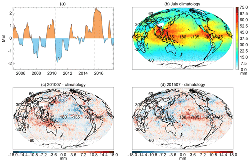
In Fig. 7, we examine the signals associated with El Niño and La Niña in version 4.0 OMI TCWV. Figure 7a shows the multivariate ENSO index (MEI) from NOAA (Wolter and Timlin, 1998) (https://www.esrl.noaa.gov/psd/enso/mei/, last access: 17 September 2019). Positive (negative) values correspond to El Niño (La Niña) conditions. We examine the anomalies in TCWV for July 2010 (MEI = −1.103, La Niña) and July 2015 (MEI = 1.981, El Niño) in Fig. 7c and d. Although these events are strong within the OMI record (from 2005 to the present), they are mild in comparison with the extrema. Between 1950 and 2018, the maximum MEI is 3.008 (in March 1983) and the minimum MEI is −2.247 (in June 1955).

To examine the changes in OMI TCWV under different conditions, we first generate the monthly Level 3 ($\mathrm{0.5}{}^{\circ }\times \mathrm{0.5}{}^{\circ }$) OMI TCWV using the Level 2 data for July 2005 and July 2015 using the method described in Sect. 3.2 (with a cloud fraction threshold of f=0.15 and a cloud-top pressure threshold of 750 mb). Then, using the same data filtering criteria, we derive the climatology for July using all the Level 2 July data between 2005 and 2015 (Fig. 7b). Finally, we plot the deviations from the climatology (mm) for July 2010 and July 2015 in Fig. 7c and d, respectively.

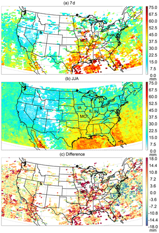
Figure 8 Level 3 ($\mathrm{0.25}{}^{\circ }\times \mathrm{0.25}{}^{\circ }$) OMI TCWV (mm) generated using the Level 2 data during (a) 18–24 July 2016 and (b) 1 June–31 August 2016. (c) The difference of (a)–(b) in millimeters. The abbreviations for the states most affected by the event are indicated in the map.

The TCWV anomalies exhibit large-scale patterns. The pattern for July 2015 largely opposes that for July 2010. Particularly, in July 2015 under El Niño conditions, TCWV is higher in the equatorial central and eastern Pacific and lower in the Indonesia region, while in July 2010 under La Niña conditions, TCWV is lower in the tropical eastern Pacific and equatorial western Pacific and higher in Indonesia and the Indian Ocean. The overall patterns largely conform to the results derived from the Hamburg Ocean Atmosphere Parameters and Fluxes from Satellite Data (HOAPS; Shi et al., 2018).

4.2 Corn sweat

“Corn sweat” refers to a hot and humid condition associated with heat waves, which results in large evapotranspiration rates in the Midwestern United States where cropland is often the dominant land usage type. Besides evaporation, transpiration by plants, such as corn, draws water from the soil to the atmosphere, enhancing the humidity and increasing the heat index. A corn sweat event from 18 to 24 July in 2016 made news in the US. This event is examined in Fig. 8 using the version 4.0 OMI TCWV.

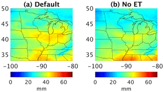
Figure 9 WRF simulations of TCWV (mm) for the Midwestern US on 21 July 2016 for the run (a) with and (b) without evapotranspiration.

Figure 8a and b show the Level 3 ($\mathrm{0.25}{}^{\circ }\times \mathrm{0.25}{}^{\circ }$) OMI TCWV for 18–24 July (7 d) and 1 June–31 August (JJA) in 2016, respectively. The 7 d period corresponds to the corn sweat event. The $\mathrm{0.25}{}^{\circ }\times \mathrm{0.25}{}^{\circ }$ Level 3 data are derived using the same filtering criteria as those used for Fig. 7. Figure 8c indicates the anomaly associated with the corn sweat event relative to the JJA mean. High TCWV is observed for the 7 d period from the Gulf Coast to the Midwestern US. Besides the gulf region, the largest TCWV enhancements (of up to 18 + mm) occur in parts of Iowa (IA), Missouri (MO), Illinois (IL) and Indiana (IN). Elevated TCWV is also observed by several GPS stations in the general area during the same time period, though coincident OMI data are not found at the stations (Fig. S3). At a few GPS stations, high TCWV persisted a couple more days after 24 July, which is most likely related to a change in the weather. As shown by the surface pressure observations at the GPS stations, the Midwest is under the control of a high-pressure system during the corn sweat period and a low-pressure system afterwards (Fig. S4).

To assess the significance of evapotranspiration for the Midwestern US during the corn sweat event, we carried out a sensitivity study using the Weather Research and Forecasting (WRF) model v3.9.1 (Skamarock et al., 2008). The model was run on a 36 km parent domain and a 12 km nested domain, covering the relevant areas of the US. The physics parameterizations included the WRF Single-Moment (WSM) 6-Class Microphysics (Hong and Lim, 2006), the Kain–Fritsch (KF) subgrid cumulus parameterization (Kain, 2004), the Yonsei University (YSU) planetary boundary layer scheme (Hong et al., 2006), the Noah Land-Surface Model (Ek et al., 2003; Chen and Dudhia, 2001) and the Rapid Radiative Transfer Model (RRTM). Horizontal turbulent diffusion was based on the standard Smagorinsky 1st-order closure. The initial and lateral boundary conditions were from the 3-hourly NCEP North American Regional Reanalysis (NARR) at 32 km resolution. To reduce the uncertainty associated with lateral boundary conditions for the nested domain, we nudged the model in the parent domain toward the reanalysis but left the nested domain running freely.

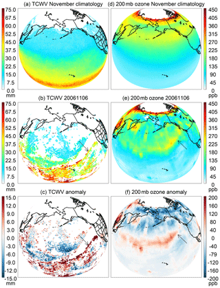
Figure 10 The Level 3 (a, d) climatology, (b, e) data on 6 November 2006 and (c, f) anomaly on 6 November 2006 with respect to the climatology for (a, b, c) version 4.0 OMI TCWV (mm; $\mathrm{0.5}{}^{\circ }\times \mathrm{0.5}{}^{\circ }$) and (d, e, f) the OMI ozone mixing ratio (ppb; $\mathrm{1}{}^{\circ }\times \mathrm{1}{}^{\circ }$) interpolated to 200 mb.

To diagnose the contribution of evapotranspiration, the model was run from 19 to 22 July 2016 with and without evapotranspiration (calculated in the Noah Land-Surface Model). The results for 21 July are shown in Fig. 9. TCWV is generally lower in the interior of the domain for the run without evapotranspiration (No ET). The higher TCWV in the No ET run near the southern boundary reflects nonlinear water vapor transport from the gulf region. Turning off evapotranspiration not only directly affects the water vapor flux from the surface but also indirectly influences other meteorological variables, such as winds. Thus, there is a difference in the water vapor flux across the domain boundary. The difference between the default and No ET runs in Fig. 9 suggests that evapotranspiration contributes about 15 %–25 % of the TCWV in the Midwestern US during the corn sweat event. A detailed study incorporating TCWV data with the WRF model will be carried out in future work.

Figure 11 (a) WRF model domain configuration for the November 2006 AR event. (b) TCWV observed by SSM/I on 6 November 2006. (c, d) TCWV simulated by WRF on the same day (c) without and (d) with OMI TCWV data assimilation. Gray indicates area with no SSM/I data.

4.3 Atmospheric river (AR)

4.3.1 An intense AR in OMI data

ARs are narrow elongated bands with high TCWV in the atmosphere. With flow rates similar to those of large rivers, ARs are highly important in the global hydrological cycle (Zhu and Newell, 1998). Landfalling ARs can lead to heavy orographic precipitation that affects areas such as the west coast of North America and Europe (Gimeno et al., 2014; Neiman et al., 2008b).

Figure 12 The simulated rainfall accumulated from 00:00 to 23:00 UTC (mm) on 6 November 2006 for the model (a) without and (b) with OMI TCWV assimilation. (c) The accumulated rainfall observed by TRMM for the same time period. Note that the 3 km model result is coarsened to match the resolution of the TRMM product. Box A highlights the erroneously simulated precipitation in the run without OMI TCWV data assimilation.

The extreme AR of 6–7 November 2006 brought devastating flood to the Pacific Northwest – the region in western North America bounded by the Pacific to the west and the Cascade Range to the east. This AR is described in detail in Neiman et al. (2008a). The signature of this AR is captured in the version 4.0 OMI TCWV data. Figure 10a–c show the Level 3 OMI TCWV and its anomaly on 6 November 2006. The Level 3 data are generated following the same procedure as that used for Fig. 8. Although many pixels are missing because of the cloud filtering (cloud-top pressure >750 mb, cloud fraction < 0.15) and other criteria, the leading edge of the AR is noticeable as an elongated band of high TCWV (15 + mm above the climatology) extending from Hawaii to northern California (indicated by arrows in Fig. 7b and c). The position of the AR in OMI TCWV agrees well with that in Special Sensor Microwave/Imager (SSM/I) microwave observations (Neiman et al., 2008a).

Figure 10d–f show the Level 3 OMI ozone mixing ratio interpolated to 200 mb and its anomaly. The OMI ozone data are retrieved using the SAO ozone profile algorithm (Liu et al., 2010; Huang et al., 2017, 2018). The climatology is derived by averaging all monthly Level 3 data for November from 2004 to 2017. The global distribution of ozone at 200 mb shows a low mixing ratio in the low latitudes and high mixing ratio in the high latitudes, opposite to the global distribution of TCWV. The anomaly shows a curvilinear band of high ozone that is parallel to the AR in Fig. 10b, c but located further to the west. This feature indicates the intrusion of ozone-rich stratospheric air along the polar front and is associated with the same extratropical cyclone as the AR.

4.3.2 OMI TCWV assimilation for the AR

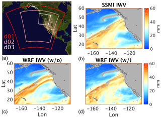
To evaluate the potential of OMI water vapor data to improve numerical weather forecasts, we conducted a data assimilation experiment from 2 to 8 November 2006 using WRF v3.9.1 and version 4.0 OMI TCWV. The model was configured with 27 km (290×270 surface grid points with 51 vertical levels), 9 km ($\mathrm{586}\times \mathrm{586}\times \mathrm{51}$ points) and 3 km ($\mathrm{541}\times \mathrm{526}\times \mathrm{51}$) nested domains in a Lambert projection over the relevant portion of the Pacific and North America (Fig. 11 top left). The domains are designed for the 6 November AR event and its associated precipitation at landfall. The model has the same physics parameterizations as those used in Sect. 4.2 except that a more sophisticated double-moment microphysics scheme is used for quantifying precipitation. The initial and boundary conditions for the 27 km domain were from the $\mathrm{1}{}^{\circ }\times \mathrm{1}{}^{\circ }$ NCEP final (FNL) reanalysis. One-way nesting is used for the inner domains. To evaluate the model's skill at simulating the AR and the contribution of OMI TCWV to the quality of the simulation, we did not nudge the run towards the reanalysis or assimilate the observed sea surface temperature within the computational domains.

The OMI TCWV is assimilated into the model using analytical optimal estimation (Rodgers, 2000). This method minimizes the cost function $J\left(\mathit{x}\right)={\left(\mathit{y}-\mathbf{H}\mathit{x}\right)}^T{\mathbf{E}}^{-\mathrm{1}}\left(\mathit{y}-\mathbf{H}\mathit{x}\right)+{\left(\mathit{x}-{\mathit{x}}^{\mathit{b}}\right)}^T{\mathbf{B}}^{-\mathrm{1}}\left(\mathit{x}-{\mathit{x}}^{\mathit{b}}\right)$, where x is the true TCWV, x^b is the a priori TCWV (from the model), y is the observed TCWV, H represents the model Jacobian, and B and E are the error covariance matrices of the a priori and observation. B is estimated with 12 and 24 h forecasts using the National Meteorological Center method (Parrish and Derber, 1992). E is based on the fitting uncertainties of OMI data.

The a posteriori analysis ($\widehat{x}$) can be obtained from $\widehat{x}=x^b+\mathbf{K}(y-\mathbf{H}x$), where $\mathbf{K}={\mathbf{BH}}^T{\left({\mathbf{HBH}}^T+W^{-\mathrm{1}}\mathbf{E}\right)}^{-\mathrm{1}}$ is the Kalman gain, $W=\frac{(R^{\mathrm{2}}-r^{\mathrm{2}})}{(R^{\mathrm{2}}+r^{\mathrm{2}})}$ is the Cressman function to weigh the observations based on their Euclidian distance r to the model grids and R is the influence radius of the observations. We simply assume R to be 1, 0.5 and 0.25^∘ for the 27, 9 and 3 km domain to get a quick look at the results in this paper and leave a more vigorous quantification of R to future work. The a posteriori TCWV is solved hourly when OMI data are available and is used to initialize the next simulation window.

During the assimilation, we adjust the OMI data using the AMF calculated with the modeled water vapor profile (${\text{OMI}}_{\text{satellite}}^{\text{adjusted}}=\frac{{\text{OMI}}_{\text{satellite}}\times {\text{AMF}}_{\text{satellite}}}{{\text{AMF}}_{\text{model}}}$) and the scattering weights provided with the Level 2 OMI data. This can reduce the observational error associated with using the monthly mean water vapor profile in the operational OMI product. The standard deviation of the difference between AMF_satellite and AMF_model is about 20 %.

Figure 11 shows zoomed-in views of the AR on 6 November 2006. The TCWV independently observed by SSM/I is shown in Fig. 11b. Figure 11c and d show the model results without and with OMI TCWV assimilation. The model without assimilation shows an AR that is split into two parallel filaments making landfall at separate locations on the west coast of North America, where the TCWV is too high compared to the SSM/I observation, especially for the southern filament. As discussed later, this has a significant impact on precipitation (Fig. 12). After assimilating OMI TCWV, the modeled TCWV agrees much better with the SSM/I observation. The spurious southern filament disappeared, and the overall shape and amplitude of the AR are significantly improved.

The location and intensity of precipitation over land are crucial for local flood control and water resource management and are closely related to the shape and strength of AR at landfall. The 24 h accumulated precipitation on 6 November in the 3 km domain is examined in Fig. 12. The model output is coarsened to $\mathrm{0.25}{}^{\circ }\times \mathrm{0.25}{}^{\circ }$ to match the resolution of the Tropical Rainfall Measuring Mission (TRMM) observation product. The model without OMI data assimilation produces spurious rainfall over the Oregon–California border (box A) as a result of the erroneously strong southern filament of the simulated AR (Fig. 11c). This artifact was removed after OMI data assimilation, showing better agreement with the corresponding TRMM rainfall observation. The difference in rainfall between the assimilation and observation in the Oregon–Washington area is probably related to both the model error and the data error, as well as the data density and distribution. A detailed error attribution for precipitation is beyond the scope of this paper.

5 Summary and conclusion

The version 4.0 retrieval algorithm for OMI total column water vapor (TCWV) is presented in this paper. The algorithm follows the usual two-step approach in which slant column density (SCD) is derived from spectral fitting and vertical column density (VCD) is obtained through the ratio of SCD and air mass factor (AMF). In version 4.0, the spectral fitting no longer considers a common mode. The retrieval window (432.0–466.5 nm) results from a systematic optimization that reflects trade-offs among several factors, including a small fitting RMS, small fitting uncertainty, large fraction of successful retrievals and long retrieval window length. The AMF calculation uses the latest OMI O₂–O₂ cloud product (Veefkind et al., 2016) and monthly variable vertical profiles from the MERRA-2 reanalysis (Gelaro et al., 2017).

The version 4.0 OMI TCWV product is compared against the GPS network data over land and the SSMIS microwave observations over the oceans for 2006. Version 4.0 OMI TCWV has a much smaller bias than version 3.0 and has replaced previous versions on the Aura Validation Data Center website. Version 4.0 OMI TCWV is characterized under different cloud conditions. Under clear-sky conditions (cloud fraction <5 % and cloud-top pressure >750 mb), the overall mean of OMI–GPS over land is 0.32 mm with a standard deviation of 5.2 mm, and the smallest bias occurs when TCWV is between 10 and 20 mm; the overall mean of OMI–SSMIS over the oceans is 0.4–1.1 mm with a standard deviation of 6.5–6.8 mm, and the smallest bias occurs for TCWV between 20 and 30 mm. The correlation coefficient between OMI TCWV and the reference datasets realizes the largest gain when the cloud fraction threshold is increased from 5 % to 15 %. The regression line appears the best when f=0.25 is used over land and when f=0.15 is used over the oceans. But, a larger cloud fraction leads to larger bias and scatter. Thus, for most applications, we recommend considering only OMI data with cloud fraction <5 % to 25 % and cloud-top pressure >750 mb, in addition to main data quality flag = 0, no row anomaly, fitting RMS < 0.001 and 0 < TCWV < 75 mm. Relaxing the cloud-top pressure threshold has a similar effect as relaxing the cloud fraction threshold. TCWV corresponding to low cloud-top pressure (high altitude) should be used with caution due to the degraded accuracy for these clouds in the OMCLDO2 product.

As example applications of the version 4.0 OMI TCWV data across a variety of temporal and spatial scales, this paper examines the climate pattern associated with El Niño–La Niña, the enhanced humidity during a week-long corn sweat event in the Midwest US and the elongated band of high TCWV associated with an intense atmospheric river that made landfall on the west coast of North America. Strong signals are found in OMI TCWV for all three examples. A data assimilation experiment shows that the OMI TCWV data can help improve WRF's skill in simulating the shape and intensity of the AR, as well as the accumulated rainfall near the coast.

Further improvement of the product can proceed from both spectral fitting and AMF calculation, such as water vapor reference spectrum, instrument slit function and solar irradiance for spectral fitting, aerosol correction and surface bidirectional reflectance for AMF calculation.