ELIFAN, an algorithm for the estimation of cloud cover from sky imagers

In the context of a network of sky cameras installed on atmospheric multi-instrumented sites, we present an algorithm named ELIFAN, which aims to estimate the cloud cover amount from full-sky visible daytime images with a common principle and procedure. ELIFAN was initially developed for a self-made full-sky image system presented in this article and adapted to a set of other systems in the network. It is based on red-to-blue ratio thresholding for the distinction of cloudy and cloud-free pixels of the image and on the use of a cloud-free sky library, without taking account of aerosol loading. Both an absolute (without the use of a cloud-free reference image) and a differential (based on a cloud-free reference image) red-to-blue ratio thresholding are used.

An evaluation of the algorithm based on a 1-year-long series of images shows that the proposed algorithm is very convincing for most of the images, with about 97 % of relevance in the process, outside the sunrise and sunset transitions. During those latter periods, however, ELIFAN has large difficulties in appropriately processing the image due to a large difference in color composition and potential confusion between cloud-free and cloudy sky at that time. This issue also impacts the library of cloud-free images. Beside this, the library also reveals some limitations during daytime, with the possible presence of very small and/or thin clouds. However, the latter have only a small impact on the cloud cover estimate.

The two thresholding methodologies, the absolute and the differential red-to-blue ratio thresholding processes, agree very well, with departure usually below 8 % except in sunrise–sunset periods and in some specific conditions. The use of the cloud-free image library gives generally better results than the absolute process. It particularly better detects thin cirrus clouds. But the absolute thresholding process turns out to be better sometimes, for example in some cases in which the sun is hidden by a cloud.

1 Introduction

Due to their crucial role in weather and climate, clouds are the focus of many observation systems all over the world. Sky imagers are naturally used as simple devices for visible-sky monitoring: they give very useful qualitative information on the state of the sky and the type of clouds. But they can also fulfill quantitative parameters after a processing of the image that is either based on the texture of the image or on the (red, green, blue) color composition of the image. Historically, some of the first systems were developed for military purposes, especially for the detection of a cloud-free line of sight (Johnson and Hering, 1987). But soon, their applications were extended to meteorology, climate, and solar energy. Ghonima et al. (2012) and Shields et al. (2013) give rich and interesting reviews of sky imager systems and their applications. Several algorithms have now been proposed that enable us to retrieve an estimation of cloud cover (e.g., Long and DeLuisi, 1998; Li et al., 2011; Ghonima et al., 2012; Martinis et al., 2013; Silva and Echer, 2013; Cazorla et al., 2015; Kim et al., 2016; Krinitskiy and Sinitsyn, 2016) or solar irradiance (Pfister et al., 2003; Chu et al., 2014; Chauvin et al., 2015; Kurtz and Kleissl, 2017), to classify the type of observed clouds (e.g., Heinle et al., 2010; Kazantzidis et al., 2012; Xia et al., 2015; Gan et al., 2017), or to track them (Peng et al., 2015; Cheng, 2017; Richardson et al., 2017). Sky imagers have also been specifically used for the detection of cirrus (Yang et al., 2012) or thin clouds (Li et al., 2012) and contrail studies (Schumann et al., 2013). Furthermore, one can also estimate cloud-base height (Allmen and Kegelmeyer, 1996; Kassianov et al., 2005; Nguyen and Kleissl, 2014) by using a pair of sky cameras.

Those systems are now commonly deployed in the vicinity of solar farms for the intra-hour or now-casting of solar irradiance and during atmospheric field experiments or on permanent observatories for cloud cover and cloud type monitoring.

Within the ACTRIS-FR¹ French research infrastructure, several instrumented permanent sites have coordinated their actions for the observation of the atmosphere and attempt to homogenize their instrumental, data process, and data dissemination practices for wider and more consistent multi-parameter data use by the international research community. In this context, a common sky imager algorithm has been developed, called ELIFAN, in order to retrieve in a similar way the cloud fraction from all the sky cameras of the different sites. It is now used on three ACTRIS-FR sites and is in progress on three other sites. ELIFAN is based on red-to-blue ratio (here after RBR) thresholding for the distinction of cloudy and cloud-free pixels of the image and on the use of a cloud-free sky library. This article aims to present the ELIFAN algorithm principles, strengths, limitations, and perspectives.

In Sect. 2, we present the sky cameras used in the ACTRIS-FR infrastructure, with more details on a self-made sky imager developed at one of the instrumented sites and on which ELIFAN was originally based. In Sect. 3, the ELIFAN algorithm is explained in detail. In Sect. 4, an evaluation of ELIFAN highlights its main strengths and limitations. We make concluding remarks in the last section, with perspectives on the evolution of the algorithm and further discussion.

2 Sky imager systems used

2.1 The sky imager systems of ACTRIS-FR instrumented sites

There are five important multi-instrumented sites that participate in the French infrastructure ACTRIS-FR and are spread over French territory.

• P2OA (Pyrenean Platform for the Observation of the Atmosphere²) is located in the Pyrénées, near the Spanish border in southwest France, with two sites: one at Pic du Midi summit (42.94^∘ N, 0.143^∘ E) and the other close to Lannemezan at the Centre de Recherches Atmosphériques (43.13^∘ N, 0.366^∘ E).

• SIRTA (Site Instrumental de Recherche par Télédétection Atmosphérique; Haeffelin et al., 2005) is located at Palaiseau, south of Paris (48.72^∘ N, 2.21^∘ E).

• CO-PDD (Cézeaux-Opme-Puy de Dôme³) is in the center of France, with three sites: one at the Puy de Dôme summit (1465 m; 45.77^∘ N, 2.96^∘ E), one at Opme (680 m; 45.71^∘ N, 3.09°E), and one at the Cézeaux University site (410 m; 45.76^∘ N, 3.11^∘ E).

• OHP (Observatoire de Haute Provence⁴) is in the Provence region in southeast France (43.93^∘ N, 5.71^∘ E).

• OPAR (Observatoire de Physique de l'Atmosphère de la Réunion⁵) is on Réunion Island (21.08^∘ N, 55.38^∘ E).

All have a sky camera for cloud monitoring, but different systems have historically been used: the TSI (Total Sky Imager, used at SIRTA from 23 October 2008 to 24 June 2015), ASI (All Sky Imager) from EKO (used at SIRTA, CO-PDD, and P2OA mountain sites), Alcor System (used at OPAR), and self-made instruments (RAPACE, used at the P2OA plain site, with another one at OHP).

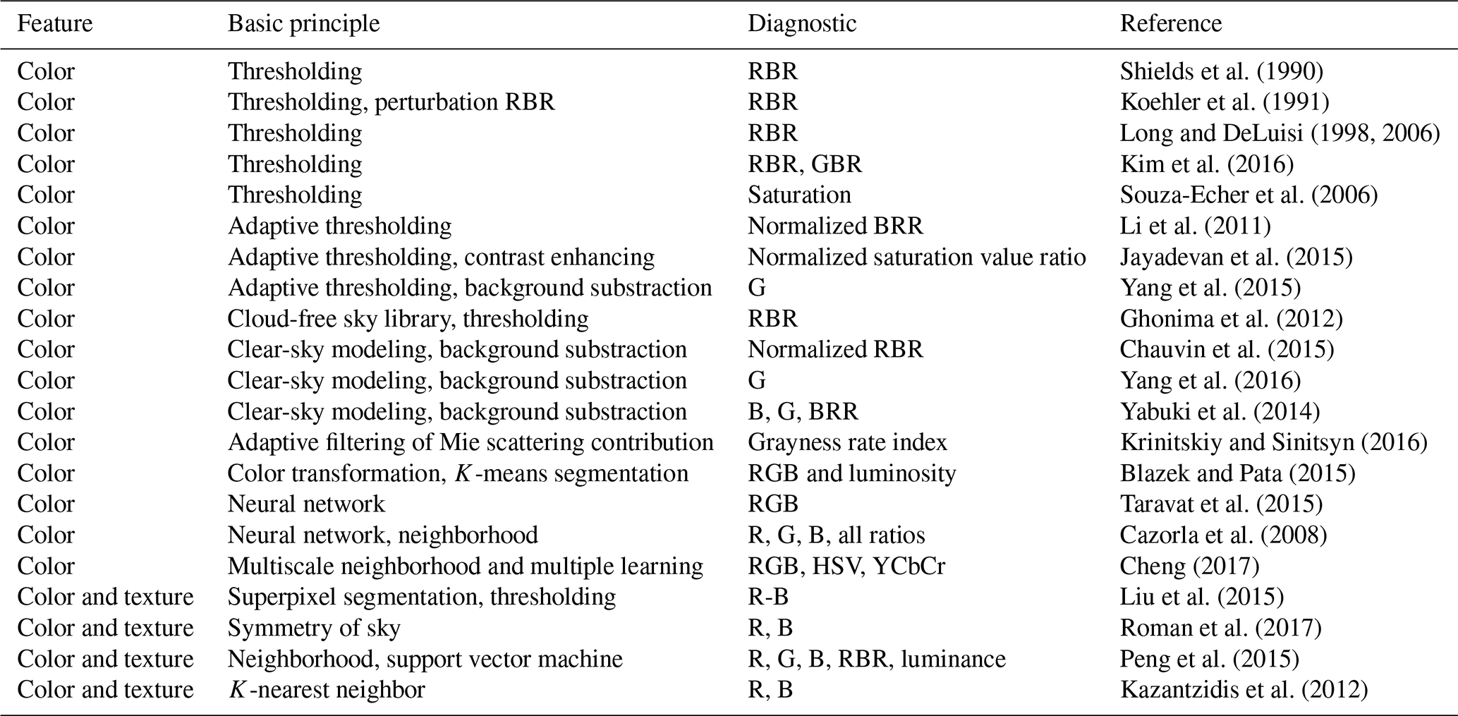
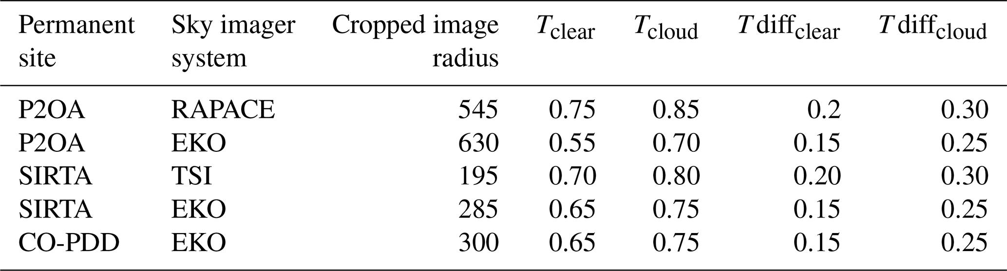
Table 1 summarizes the systems used at three observatories where sky images are currently processed for cloud cover retrieval.

Table 1 List of sky imager systems within the ACTRIS-FR infrastructure and their characteristics. The list here only considers the systems for which the images are processed by ELIFAN for cloud cover retrieval.

Initially, the image processing algorithm was developed and thoroughly evaluated on RAPACE system images. But it was subsequently adapted for the other commercial systems in order to realize a common data process within the ACTRIS-FR sky imager network.

In the following subsection, we describe in more detail the RAPACE self-made system that is at the origin of the ELIFAN algorithm development and which will be considered for the illustrations in further sections.

2.2 RAPACE system

There are several self-made systems presented in the literature that show that this is often a quite satisfactory option when trying to acquire good-quality images at significantly lower cost than commercial systems. The developers then also design their own specific data process, depending on their objectives.

Shields et al. (2013) give a historical and experienced-based overview of the development and use of the Whole Sky Imager (WSI) first deployed in 1984 (Johnson et al., 1989), later improved into the day–night whole-sky imager (D/N) WSI (first deployed in 1992, Shields et al., 1993) at the University of California, San Diego, USA. The WSI used a charge injection device (CID) solid-state imager and a fish-eye lens. The D/N WSI is based on a Photometrics slow scan charge-coupled device (CCD) camera and a fish-eye lens. It is capable of detecting cloudy and cloud-free sky in starlight, moonlight, and daytime (through the ratio of near-infrared to blue).

Most of the systems developed in the last decade are similarly based on a digital camera coupled with an upward-looking fish-eye lens (e.g., Souza-Echer et al., 2006; Seiz et al., 2007; Calbó and Sabburg, 2008; Jayadevan et al., 2015). Cazorla et al. (2008) used a CCD camera for the purpose of cloud cover estimation and characterization. The system captures a multispectral image every 5 min. Kazantzidis et al. (2012) made a whole-sky imaging system based on a commercial digital camera with a fish-eye lens and a hemispheric dome for the automatic estimation of total cloud coverage and classification. Chu et al. (2014) proposed an automatic smart adaptive cloud identification (SACI) system for sky imagery and solar irradiance forecast, which uses an off-the-shelf fish-eye objective. Urquhart et al. (2015) developed a high dynamic range (HDR) camera system capable of providing a full-sky multispectral image at radiometric resolution every 1.3 s.

An alternative design, instead of a fish-eye lens, uses a spherical mirror and a downward-looking camera fixed above. Such systems were also historically developed in the late 1970s or early 1980s, like that mentioned in Benech et al. (1980). This type of design is used in several recent developments (e.g., Pfister et al., 2003; Long et al., 2006; Mantelli Neto et al., 2010; Chow et al., 2011).

The instrument used at the P2OA plain site, called RAPACE (Récepteur Automatique Pour l'Acquisition du Ciel Entier) was made in December 2006 at low cost based on the first type of design and similar to Kazantzidis et al. (2012) with the purpose of taking automatic and regular whole-sky images. The RAPACE system is composed of

• an A510 CANON camera that is remotely controllable,

• a Nikon FC-E9 fish-eye objective for full-sky images,

• a waterproof box for protection of the camera outside,

• a square board support to put the camera at the right height into the box,

• a Plexiglas dome to protect the fish-eye objective from hail, animals, and other sources of damage,

• a thermostatted heating wire to limit condensation and frost inside the dome,

• a control computer, and

• a Power Shot Remote software (from Breeze Systems) for remote control of the camera.

A picture of RAPACE is shown in Fig. 1 on the roof of the P2OA plain site laboratory building. Examples of images are shown in Fig. 2.

It has now been running since December 2006 with no significant interruption and turned out to be a very robust system, with high-quality 3.2-megapixel images taken every 15 min until February 2017 and every 5 min (during daytime, 15 min during nighttime) since then.

Assuming that the main fragility would lie in the mechanical constraint endured during (i) the successive opening and closing of the digital camera objective and (ii) focusing, we have blocked the objective in the opened position and also fixed the focus after focusing to infinity. This seemed to help a lot in the system endurance, as RAPACE has run for 12.5 years now with the same original digital camera and fish-eye objective. Only the Plexiglas dome has been replaced a couple of times due to hail damage, and the USB extension wires have been improved over time.

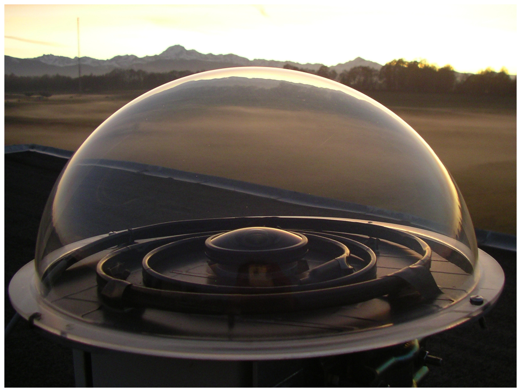
Figure 1 The RAPACE sky imager system developed at the P2OA instrumented site. We can see the fish-eye lens at the center, the Plexiglas dome, and the thermostatted heating wire in a spiral around the fish-eye.

With the purpose of using a common and centralized data process to retrieve cloud cover from the images of all the sky cameras available at the instrumented sites of ACTRIS-FR, an algorithm has been developed. It is now operationally running at the AERIS data center for the images of all the EKO systems listed in Table 1 and of RAPACE. This algorithm is presented in detail in the next section.

Figure 2 Two examples of RAPACE full-sky images. (a) Cirrus clouds on 2 October 2007, (b) cumulus clouds on 20 February 2006. East is on the right side of the image, and north is at the bottom.

3 ELIFAN algorithm

3.1 Background on the retrieval of cloud cover from a visible-sky camera

They are several ways to detect clouds and estimate the cloud cover percentage from a visible full-sky image. Table 2 summaries the different methodologies found in the literature. Most of the algorithms rely on the color information of the image pixels, but there are also techniques based on the texture of the image. Combining both increases the retrieval capacity and especially gives more possibility for cloud type identification.

Within the first category, one simple and quite efficient way to proceed is based on the use of fixed thresholds on the RBR (Shields et al., 1990; Long and DeLuisi, 1998; Long et al., 2006). This methodology is based on the fact that a cloud-free sky is characterized by pixels with a larger contribution of blue relative to the other two colors, while clouds have more homogeneous relative contributions (closer to white or gray). The methodology can be sophisticated with the combination of RBR and GBR (green-to-blue ratio) (Kim et al., 2016) or the use of saturation (Souza-Echer et al., 2006). One of the main difficulties lies in the variability of the color of the cloud-free sky from one day to another (for example, due to variable aerosol loading and hydration) and from one time to another (due to variable sun elevation). The use of adaptive thresholding (Li et al., 2011; Jayadevan et al., 2015) helps improve the results in this respect. Another permanent challenge is due to the variability of the color of cloud-free sky from one part of the image to another. There is indeed heterogeneity within a totally cloud-free image due to forward scattering and Mie scattering of aerosols. Depending on the position of the pixel relative to the sun position, the cloud-free sky appears differently. It especially makes the circumsolar area very difficult to deal with (there is an increase in whitening around the sun). To solve this issue, Ghonima et al. (2012) use a real cloud-free sky library as a reference, composed of a set of cloud-free sky images found within a large dataset. The difference between the RBR of the processed image and the RBR of a reference cloud-free image (with similar elevation and azimuth solar angles) differentiates the cloudy pixels from the cloud-free pixels. Going further, recent methodologies based on background substraction take account of the clear-sky spatial and temporal variability through the use of a modeled (or so-called “virtual”) clear sky (Yabuki et al., 2014; Chauvin et al., 2015; Yang et al., 2016). Note that Koehler et al. (1991) already used a “perturbation” ratio of RBR, relative to a haze-adjusted background RBR, to optimize thin cloud detection.

Mathematical tools like neural networks, K-nearest neighbor techniques, and support vector machines (SVMs) are also used for cloud detection based on RGB composition and luminosity (Blazek and Pata, 2015; Taravat et al., 2015; Cheng, 2017) and on the image texture (Cazorla et al., 2008; Kazantzidis et al., 2012; Liu et al., 2015; Peng et al., 2015). The combination of both allowed Kazantzidis et al. (2012) to distinguish seven types of clouds, in addition to estimating cloud cover amount. Roman et al. (2017) interestingly use the fact that an image of totally clear sky is symmetric.

Finally, there is of course a gain in combining instruments. Ceilometers and sky imagers are very complementary in this respect, as the ceilometer adds cloud-base height information above the sky camera system (Chu et al., 2014; Roman et al., 2017), which can allow for access to cloud speed motion (Wang et al., 2016). Pyranometers are also naturally considered in such instrumental synergy (Peng et al., 2015; Wang and Kleissl, 2016).

Shields et al. (1990)Koehler et al. (1991)Long and DeLuisiKim et al. (2016)Souza-Echer et al. (2006)Li et al. (2011)Jayadevan et al. (2015)Yang et al. (2015)Ghonima et al. (2012)Chauvin et al. (2015)Yang et al. (2016)Yabuki et al. (2014)Krinitskiy and Sinitsyn (2016)Blazek and Pata (2015)Taravat et al. (2015)Cazorla et al. (2008)Cheng (2017)Liu et al. (2015)Roman et al. (2017)Peng et al. (2015)Kazantzidis et al. (2012)

Table 2 Synthetic table of background studies of cloud cover retrieval algorithms from a daytime visible-sky camera.

3.2 Principle and methodology of ELIFAN algorithm

Initially developed in 2013, the ELIFAN algorithm aims to estimate the cloud cover percentage during daytime based on a visible image. At that time, only the RAPACE system at the P2OA site and the TSI-440 system at the SIRTA site were used within the network of instrumented sites. An algorithm that could be used for both cameras, despite their differences, needed to be developed. ELIFAN is basically inspired by Ghonima et al. (2012), with the use of the RBR as the driving diagnostic to differentiate cloudy and cloud-free pixels by thresholding and of a reference cloud-free sky library. Considering the literature overviewed before, ELIFAN's innovation is limited. One originality of ELIFAN, however, is that it applies both an absolute and a differential thresholding process independently. Each of them has advantages and drawbacks, but both are complementary.

Figure 3 (a) Initial image on 26 February 2014 at 13:00 UTC. (b) Corresponding cropped image (step 1 of the process). In (a), the black circles indicate the contour of the cropped image shown in (b), outside which the pixels are not processed. In (b), the black circle indicates the contour of the sun mask, within which the pixels are not processed.

3.2.1 The different steps along the process

For a given image to be processed, the different steps are the following.

• Step 1: the image is cropped in order to remove the obstacles at the horizon and the circumferential part of the image that is too distorted and cannot be properly interpreted. The cropped area is fixed and corresponds to an aperture angle of 143^∘ centered toward zenith. Figure 3 shows an example of a raw RAPACE image (26 February 2014 at 13:00 UTC) and the corresponding cropped selection (step 1). Only the pixels located in the cropped image (i.e., inside the black circle in Fig. 3a) are processed.

• Step 2: a solar mask is applied, as are other masks if needed (e.g., for the TSI camera, which has a sun mask arm). The solar mask is positioned based on the solar zenith and azimuth angles, which are calculated with the algorithm given by Reda and Andreas (2003) as a function of the localization of the site, the date, and the time. The coordinates of the sun in the cropped image, I_s and J_s, are then calculated with the solar angles and taking account of the deformation due to the fish-eye lens:

  $$\begin{array}{}\text{(1)}& \begin{array}{rl}& I_{\mathrm{s}}=\text{Int}\left(\mathrm{A}-\mathrm{B}\sin (\mathit{\alpha }/\mathrm{2})\cos \mathit{\theta }\right)\\ & J_{\mathrm{s}}=\text{Int}\left(\mathrm{A}-\mathrm{B}\sin (\mathit{\alpha }/\mathrm{2})\sin \mathit{\theta }\right)\end{array}\end{array}$$

  where θ is the solar azimuth angle (from north toward the east), α is the solar zenith angle, and A and B are adjusted according to the camera. The diameter of the sun mask is a compromise between loosing some processed pixels, and increasing the error due to circumsolar area. The sun mask diameter here is about three times the sun disk diameter. The sun mask represents 10 % of the cropped processed image, when it is entirely included in the cropped image.

• Step 3 (see Sect. 3.2.2): with a combination of criteria applied on the global probability density function (PDF) of the image RBR, a primary phase evaluates whether the image is totally cloudy, totally free of cloud, or partly cloudy.

  • A totally cloudy image is associated with 100 % cloud cover.

  • A totally cloud-free image is sent to the cloud-free sky library and associated with a 0 % cloud cover.

  • A partly cloudy image continues the process with the following step.

• Step 4 (see Sect. 3.2.3): as a secondary phase, all images considered partly cloudy during the previous step 3 are processed from a pixel-by-pixel point of view. For this, the algorithm searches for a reference cloud-free sky image within a library, with the sun at the same azimuth and same elevation, $\pm \mathrm{1}{}^{\circ }$, as the considered image.

  • If there is no reference image, the image is processed with the absolute RBR threshold process.

  • If there is a reference image, the image is processed with both the absolute RBR threshold process and the differential RBR threshold process. If there are several reference images available, the sky with the least turbidity is chosen as a reference based on the RBR PDF.

  Cloud cover estimate is given by the percentage of cloudy pixels, uncertain pixels, and cloud-free pixels.

A schematic of the pathway, following the image and with a summary of the steps, is presented in Fig. 4, and steps 3 and 4 mentioned above are explained and illustrated in more detail in the following subsections.

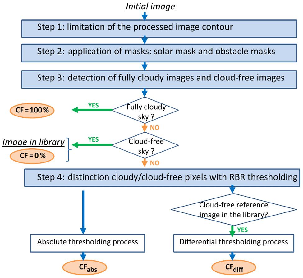
Figure 4 Organigram of the various steps in the image processing procedure. CF_abs is the cloud fraction deduced from the absolute thresholding process, and CF_diff is the cloud fraction deduced from the differential thresholding process.

3.2.2 Step 3: detection of cloud-free sky and fully cloudy-sky images

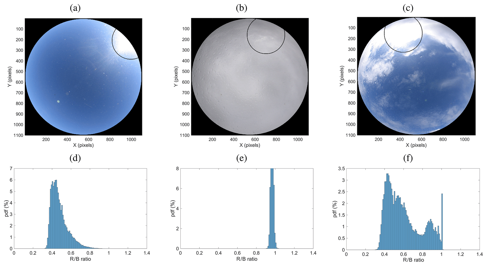
Figure 5 Cropped images of (a) 17 February 2014 at 08:30 UTC, (b) 26 February 2014 at 11:00 UTC, (c) 26 February 2014 at 13:00 UTC, and (d, e, f) the corresponding PDF of the RBR, respectively.

In step 3, the principle is to consider the cropped image as a whole and detect whether it is a fully cloudy-sky image, a fully cloud-free sky image, or neither of those two (i.e., a partly cloudy image). This step is based on the RBR distribution of the entire ensemble of pixels.

Figure 5 shows three examples: an image without cloud (Fig. 5a), a second with fully cloudy sky (Fig. 5b), and a third with partly cloudy sky (Fig. 5c, which is the same as in Fig. 3). In the first image (cloud-free sky; Fig. 5a), all the pixels have RBR <0.75. The spread from 0.3 to 0.8 is due to the variability of the RBR with the scattering angle from zenith. Ghonima et al. (2012) have shown how the RBR in a given circular band of a cloud-free sky image also depends on the 500 nm aerosol optical depth (AOD), varying almost linearly with AOD from 0.3 to 0.6 in their analysis for AOD within [0, 0.3] for a scattering (zenith) angle within 0.35–0.45^∘.

In the second image (fully cloudy; Fig. 5b), most of the pixels have RBR >0.75. Thicker clouds have RBR closer to 1 (Ghonima et al., 2012).

In the third image (partly cloudy; Fig. 5c) the probability density function (PDF) of the RBR shows a bimodal distribution, corresponding to the two sets of cloud-free pixels on the one hand (left-side peak in the distribution) and cloudy-sky pixels on the other hand (right-side peak).

The main goal of step 3 is to detect whether the image is a fully cloudy image (CF = 100 %) or whether it is a cloud-free sky image to be transferred to the library.

If the maximum of RBR over the entire image is smaller than 0.6 (the case of darkened cloudy sky at sunrise or sunset) or if more than 98 % of the pixels have RBR >0.75 (like in Fig. 5b), then this image is defined as a fully cloudy image.

Otherwise, we check whether the image has less than 2.5 % of the pixels with RBR >0.75 but still a few pixels with RBR >0.85. A cloud-free image meets this criterion because it has most of its pixels with RBR <0.75 (see Fig. 5a), but due to a few white pixels in the circumsolar region (around the sun mask here), there will be a few pixels with very high RBR (>0.85).

So we then verify whether the image has some cloudy pixels or is really cloud-free. If it meets at least two criteria among the following three criteria, it means that there are clouds in the image:

• more than 90 % of the pixels have RBR within [0.45, 0.65];

• the maximum probability within the [0.45, 0.65] range is larger than 35 %; and

• less than 12.5 % of the pixels have RBR ≤0.5.

Any image detected as a full cloud-free image after this test (that is, no cloud has been detected with the previous test) is sent to the cloud-free image library and associated with the azimuth and solar zenith angle corresponding to the site and time of the image. That is how the reference library is progressively built.

At this point, any image that was not detected as a fully cloudy-sky image or as a cloud-free sky image will be going through the process of step 4 for the estimate of the cloud fraction.

Note that the criteria explained above vary according to the sky camera. But they are all based on the RBR distribution over the entire set of pixels and on the same main principle. The criteria remain the same all along the day.

3.2.3 Step 4: distinction of cloudy and cloud-free pixels in a partly cloudy image

In step 4, the considered image, which is partly cloudy, is now considered from a pixel point of view, i.e., processed pixel by pixel, contrarily to step 3. It is independently submitted to both an absolute thresholding process and a differential thresholding process when there is a reference cloud-free image.

• The absolute thresholding process compares the RBR of each pixel to two thresholds, T_clear and T_cloud (with “clear” meaning cloud-free here).

  If RBR ≤T_clear, the pixel is considered cloud-free, but

  if RBR ≥T_cloud it is considered “cloudy”;

  otherwise (for $T_{\text{clear}}\le \text{RBR}\le T_{\text{cloud}}$), the pixel is said to be “uncertain”.

  For the RAPACE imager, T_clear=0.75 and T_cloud=0.85. As an example, Long et al. (2006) used a unique threshold of 0.6.

• The differential thresholding process compares the RBR difference between the considered pixel and the corresponding pixel of a reference image to two thresholds, Tdiff_clear and Tdiff_cloud.

  If RBR–RBR_lib≤Tdiff_clear, the pixel is considered cloud-free, but

  if RBR–RBR_lib≥Tdiff_cloud it is considered “cloudy”;

  otherwise (for Tdiff${}_{\text{clear}}\le {\text{RBR–RBR}}_{\mathrm{lib}}\le T{\mathrm{diff}}_{\text{cloud}}$), the pixel is said to be “uncertain”.

  For the RAPACE imager, Tdiff_clear=0.2 and Tdiff_cloud=0.3.

Figure 6 gives an example of an image processed with both the absolute (Fig. 6c, e, g) and the differential (Fig. 6d, f, h) processes. The results for this example are 78 % (84 %) cloudy pixels, 15 % (10 %) cloud-free pixels, and 7 % (6 %) uncertain pixels for the absolute (differential) process. The uncertain “pixels” correspond to pixels that are difficult to define as cloud-free or cloudy. They usually correspond to thin cirrus or to the border of a cloud. In this example, a stratocumulus cloud occupies most of the image, but a thinner cirrus cloud above it can be seen in the lower part of the image. This thin cirrus is not defined as cloud by the absolute thresholding but is partly identified through the uncertain pixels. However, it is entirely classified as a cloud by the differential process. Depending on the aim of an analysis, one may use one or the other result or even utilize the difference for complementary information and the detection of thin clouds.

Note that the reference image in Fig. 6b has some very thin cirrus clouds in the left (west–southwest). This happens sometimes when the cloud is small and thin. They may have an impact of a few percent in the final cloud cover estimate. (Note that they have no impact in the case shown here due to the thresholds.) This uncertainty will be addressed further in Sect. 4.

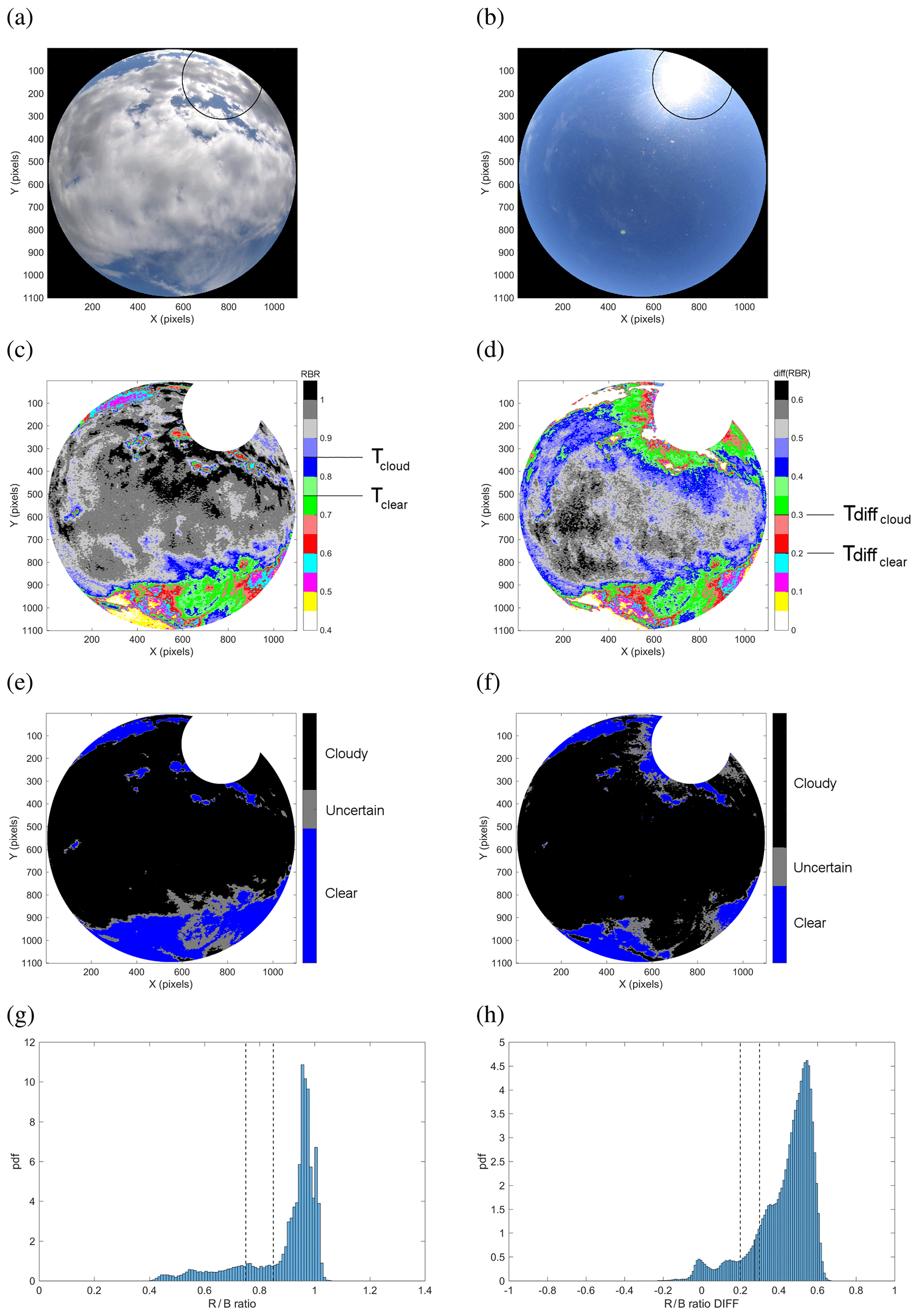
Figure 6 (a) Cropped image of 13 February 2018 at 10:30 UTC. (b) Cropped reference image used for the differential process; 12 February 2014 at 10:30 UTC. (c) RBR of cropped image (a) (for absolute process). (d) RBR difference between image (a) and reference image (b) (for differential process). (e) Result for cloudy, cloud-free, and uncertain pixels from the absolute process. (f) Result for cloudy, cloud-free, and uncertain pixels from the differential process. (g) PDF of the RBR in the initial cropped image (see c). (h) PDF of the RBR difference between the initial cropped image and the referential cropped image (see d). In (g), the black dashed lines correspond to the thresholds T_clear=0.75 and T_cloud=0.85. In (h), they correspond to the thresholds Tdiff_clear= 0.2 and Tdiff_cloud=0.3. In (c), (d), (e), and (f), “clear” means cloud-free.

3.3 Adaptation to other cameras

This algorithm was first developed for the RAPACE imager, which had no integrated process algorithm, and was then adapted to other cameras of the ACTRIS-FR instrumented sites for homogeneity of the data process within the ensemble of sites. The raw images of all sites are automatically sent to the AERIS, where ELIFAN runs and generates for each system the corresponding libraries, the cloud cover netcdf data file, and the intermediate products (RBR or RBR difference images, like in Fig. 6c and d, and the tricolor images of the cloudy, cloud-free, and uncertain pixel distribution like in Fig. 6e and f).

Table 3 Thresholds used in step 4 for the different systems of the ACTRIS-FR instrumented sites.

According to the systems, the image may differ in terms of geometry, color, or obstructing objects. Below are the camera-dependent aspects that need to be adjusted or defined in ELIFAN for it to run on a new full-sky camera.

• The geographical coordinates and type of system (fish-eye lens and camera) determine the solar mask position and course along time.

• Specific additional masks are needed for certain cameras.

• The image center and radius, as well as the radius of the cropped image, need to be determined.

• The RBR PDF criteria, which determine whether an image is fully cloudy, fully cloud-free, or partly cloudy (see step 3 above), are needed.

• RBR absolute and differential thresholding ratios, which vary from one camera to another, need to be optimized (see step 4 above).

The adaptation has been done for the EKO cameras listed in Table 1 and for the former TSI systems of SIRTA. The optimized thresholds used are indicated in Table 3. Those thresholds and those used in step 3 were optimized at ±0.05 through a sensitivity study based on 1 or 2 months of data for each camera.

One can notice different values of thresholds within the EKO systems, with smaller thresholds for the P2OA EKO camera relative to the other two EKO cameras. This is likely due to the altitude of the P2OA EKO (2877 m a.s.l.), associated with less aerosol, which shifts the cloud-free image RBR PDFs toward smaller RBR values.

From the Aerosol Robotic Network (AERONET) observations (Holben et al., 1998), Ghonima et al. (2012) showed, as mentioned before, that the RBR of a TSI camera cloud-free sky image for a scattering (zenith) angle within 0.35–0.45^∘ varies close to linearly with the 500 nm AOD, with a regression line of RBR $=\mathrm{0.87}{\mathit{\tau }}_{\mathrm{500}}+\mathrm{0.4}$ (where τ₅₀₀ is the 500 nm AOD). Even if not directly applicable, this would imply that the RBR in cloud-free sky may reach the threshold T_clear of 0.7 (used for SIRTA TSI camera) for AOD around 0.35 (and T_cloud of 0.8 for AOD around 0.46). Based on the ReOBS dataset (Chiriaco et al., 2018), with hourly AERONET 500 nm AOD data measured at SIRTA, we estimated to 7 % (2 %) the percentage of occurrence of hourly AOD larger than 0.35 (0.5) over a 10-year-long period (with 10 000 values due to missing data). This is a small percentage, but it is not negligible. We checked that the results of ELIFAN on the corresponding images remain largely satisfying, with the correct interpretation of cloud-free versus cloudy pixels, except that the misinterpreted circumsolar region is larger than on days with smaller AOD.

A climatology made over 49 sites over the world (including the SIRTA site) by Ningombam et al. (2019), based on monthly AERONET data, shows that the climatological range of AOD observed at SIRTA is similar to that of other sites (see Fig. 3 in Ningombam et al., 2019).

This shows that the RBR thresholds used in ELIFAN for the ACTRIS-Fr cameras should be suited to a relatively large spectrum of conditions for clear sky and sites, with the presence of aerosols in the typical range, even if adaptive thresholds would likely be the most appropriate to manage the aerosol and haze variability. Sites like the Izaña Observatory, with frequent heavy dust events in summer (Garcia et al., 2016) and daily AOD sometimes reaching values larger than 0.7, should be the most challenging, especially during summer.

Table 4 Eye evaluation of the performance of the ELIFAN algorithm: percentage of successful processed images in various situations or aspects over the entire year. The total number of images of the considered ensemble is specified in each evaluation.

4 Evaluation of the algorithm, strengths and limitations

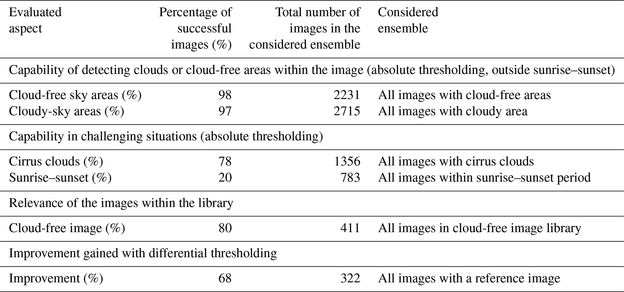
An entire year of RAPACE data (2014) has been used for ELIFAN direct evaluation before its adaptation to other systems. Instead of considering all 15 min interval images, we considered only one image out of four throughout the seasonal cycle, which resulted in a set of 4925 processed hourly images that are thoroughly evaluated. The resulting tricolor images of the cloudy, cloud-free, and uncertain spatial distribution of pixels were compared one by one to the initial images and evaluated with the human eye by a single operator (that is, without a quantified estimate of the actual number of successful pixels). Several aspects were systematically considered for this evaluation, focused on specific previously identified potential failures:

• detecting cloud-free parts of the sky,

• detecting cloudy parts of the sky,

• detecting fully cloud-free images (that is, feeding the library),

• linked with thin cirrus clouds,

• in the sunrise–sunset transition periods (±1 h around sunrise or sunset time),

• due to the reflection and refraction of the sun, and

• due to raindrops on the Plexiglas dome.

The main results of this evaluation are given in a synthetic way for the entire year in Table 4 through a percentage of successful processed images over the relevant ensemble of images. The absolute thresholding process is considered first for several specific aspects. The differential thresholding process is evaluated with the relevance of all images classified as cloud-free images and by checking that using the library improves the image analysis (and therefore the resulting cloud cover estimate).

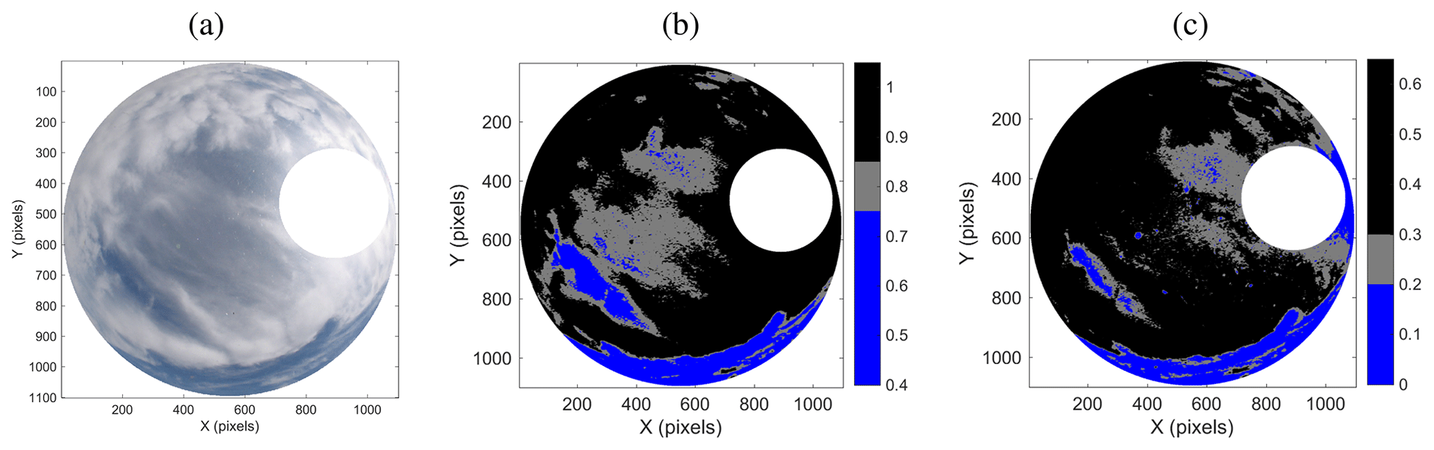
Figure 7 (a) Cropped image of 3 June 2016 at 08:30 UTC. (b, c) Result for cloudy, cloud-free, and uncertain pixels from the (b) absolute process and (c) differential process.

From this human-eye evaluation, we deduced that outside dawn and twilight times, cloudy and cloud-free parts of the sky are well identified by the absolute process, with 97 % and 98 % success, respectively, in the analysis (see Table 4). In other words, for 97 % of the studied images, the evaluator was generally satisfied with the absolute ELIFAN process in detecting the cloudy areas, without a quantified estimate of the successful versus failing pixels. Condensation and raindrops generally have no significant impact on the cloud cover estimate, and the number of images that are significantly impacted is about 20 out of the 4925 processed images. So ELIFAN works generally very well.

However, there are clearly identified limitations: dawn and twilight periods (corresponding to 16 % of the images) are critical times, with an obvious failure of the algorithm because “cloud-free sky” is not “blue” then, and clouds are not “white or gray” (80 % failure; see Table 4). The 80 % of problematic images are separated into 60 % with strong failure (in which the sky can be estimated as totally or largely cloudy instead of clear or weakly cloudy) and 20 % with small error. This is the main weakness of the algorithm and the main prospective for progress to put effort into.

Figure 8 (a) Cropped image of 7 March 2018 at 11:00 UTC. (b, c) Result for cloudy, cloud-free, and uncertain pixels from the (b) absolute process and (c) differential process.

The cloud-free sky reference library can also be improved: 80 % of the images are absolutely cloud-free. But 20 % of the images in the library are found to be inappropriate (see Table 4). Some of them (about one out of six) belong to the critical dawn–twilight period. In this latter case, the failing image may be 100 % cloudy rather than cloud-free. For all other inappropriate reference images (17 % of the reference images), only very small and/or thin clouds are present (like in Fig. 6b), so the impact on the cloud amount estimate is small.

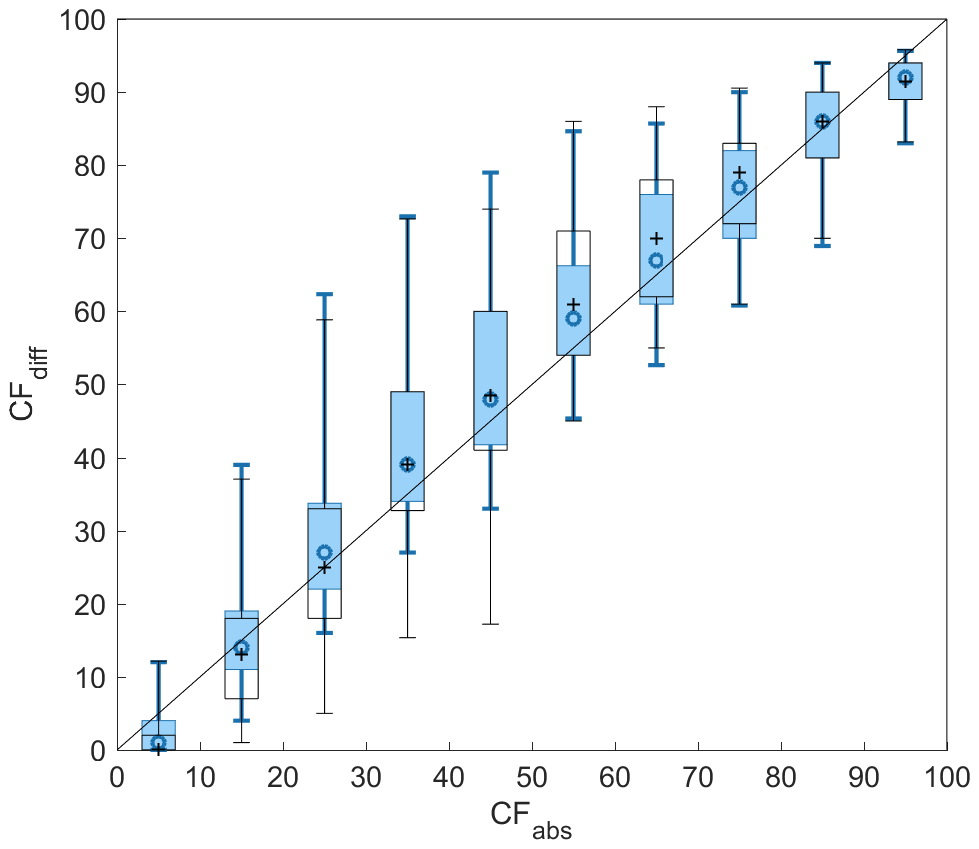
Figure 9 Comparison of the cloud fraction estimates deduced from the two thresholding processes over a set of more than 13 000 images taken during 1 year (black) at any time of the day and (blue) only during midday (between 09:00 and 15:00 UTC). CF_diff as a function of CF_abs is shown by box plots changing with bins of CF_abs values at 10 % increments. Boxes represent the 25th–75th percentile interval, and the vertical lines show the limits of the 5th and 95th percentiles. The symbol in the box stands for the median.

A total of 68 % of the time, the differential process is judged better than the absolute process (see Table 4). It gives better results in detecting cloud-free areas in the circumsolar region and also in detecting thin cirrus clouds.

The latter is illustrated in Fig. 7. In this case, quite extended thin cirrus clouds are observed in the middle of the image (Fig. 7a). Deeper cirrus clouds surround them. The absolute threshold finds a large number of uncertain pixels within the thin cirrus cloud area (Fig. 7b), while the absolute threshold process considers them cloudy pixels (Fig. 7c). So if one wants to consider those clouds in the overall cloud cover, the differential process is better. Note that the number of uncertain pixels in the absolute process interestingly gives, in this specific case, an estimate of the thin cirrus cover relative to the rest of the cloud cover.

One interest of the differential process is to deal with the circumsolar region and not interpret the white pixels in this region as clouds when the sky is cloud-free around the sun. This is indeed what we find. But when the sun is hidden by clouds, the reverse effect happens: cloudy pixels in this region can be interpreted as cloud-free by the differential process. An example of this effect is shown in Fig. 8, in which the absolute process does better in the circumsolar region than the differential process.

In addition to the previous systematic evaluation, a general statistical analysis over 1 year of data (2016) without decimating (more than 13 000 images) was made on the departure between the cloud fraction deduced from the absolute thresholding process (CF_abs) and the cloud fraction deduced from the differential thresholding process (CF_diff). The median of the difference in the percentage of cloud is 2 %. The 10 % and 90 % quantiles of the departure are respectively at −7 % and 9 %; 8 % of the values of $|{\text{CF}}_{\text{diff}}-{\text{CF}}_{\mathrm{abs}}|$ are larger than 10 %. And this latter number drops to 3 % of the images when we consider only the period of the day between 09:00 and 15:00 UTC; that is, when avoiding the tricky period of sunrise and sunset (this period corresponds to the following ranges of solar zenith angle: 20–42^∘ for the shortest winter day and 66–78^∘ for the longest summer day). Thus, large values of the departure $|{\text{CF}}_{\text{diff}}-{\text{CF}}_{\text{abs}}|$ are associated with this transition period issue, thin cirrus occurrence, and other specific situations that would lead to outliers. Figure 9 shows the correlation between CF_diff and CF_abs for this same large set of images. Considering only the midday period (thereby avoiding the dawn–twilight period) improves the correlation and 1-to-1 correspondence.

5 Concluding remarks

From the evaluation of ELIFAN with a 1-year-long data compilation, we deduced that outside the morning sunrise and sunset transitions, ELIFAN is an efficient algorithm to evaluate the cloud cover amount from a full-sky camera; 97 % of the daytime images with cloudy areas and 98 % of images with cloud-free areas are analyzed appropriately. So ELIFAN works generally very well.

However, the sunrise–sunset transition is the main weakness of the algorithm. This is where efforts should be devoted in the future for the improvement of ELIFAN. Specific criteria and thresholding could be applied in this time window.

Another limitation of ELIFAN is that a significant number of library images are not perfectly cloud-free. But, outside the critical sunrise–sunset period, it usually does not strongly impact the final cloud cover amount. The differential and absolute processes remain very consistent.

The use of the cloud-free sky library in the differential thresholding process generally improves the image process relative to the absolute process. It particularly better detects thin cirrus clouds. But the absolute thresholding process turns out to be sometimes better, depending on the conditions and on the reference image. It is also definitely useful for days with no reference image or in the case of casual field experiments for which there is no cloud-free image library available. Moreover, the combination of both estimates may be an interesting way to access the estimate of thin cirrus clouds relative to the rest of the cloud cover. But this remains to be further evaluated.

As a further development of ELIFAN, a more accurate positioning of the sun on the image will be considered, for example using the Lambert projection for the representation function that takes account of the fish-eye lens deformation, like in Crispel and Roberts (2018). In order to better take account of the presence of aerosol, the selection of the reference image in the case of multiple choices could correspond to an average turbidity rather than a minimum. Finally, an adaptive threshold method should be tested in order to better manage the variability of aerosol and haze on a given site and from one site to another.

The effort of developing a common sky image data process for a network of sky imagers has been fruitful, as five cameras of the ACTRIS-FR French multi-instrumented sites now have their images processed and gathered together at the same national data center of AERIS (at https://actris.aeris-data.fr/data/, last access: 27 September 2019). Three more cameras (on three other sites) should join soon.