the Creative Commons Attribution 4.0 License.
the Creative Commons Attribution 4.0 License.
 | 23 Oct 2019
Underestimation of column NO2 amounts from the OMI satellite compared to diurnally varying ground-based retrievals from multiple PANDORA spectrometer instruments
Nader Abuhassan
Jhoon Kim
Manvendra Dubey
Marcelo Raponi
Maria Tzortziou
Retrievals of total column NO2 (TCNO2) are compared for 14 sites from the Ozone Measuring Instrument (OMI using OMNO2-NASA v3.1) on the AURA satellite and from multiple ground-based PANDORA spectrometer instruments making direct-sun measurements. While OMI accurately provides the daily global distribution of retrieved TCNO2, OMI almost always underestimates the local amount of TCNO2 by 50 % to 100 % in polluted areas, while occasionally the daily OMI value exceeds that measured by PANDORA at very clean sites. Compared to local ground-based or aircraft measurements, OMI cannot resolve spatially variable TCNO2 pollution within a city or urban areas, which makes it less suitable for air quality assessments related to human health. In addition to systematic underestimates in polluted areas, OMI's selected 13:30 Equator crossing time polar orbit causes it to miss the frequently much higher values of TCNO2 that occur before or after the OMI overpass time. Six discussed Northern Hemisphere PANDORA sites have multi-year data records (Busan, Seoul, Washington DC, Waterflow, New Mexico, Boulder, Colorado, and Mauna Loa), and one site in the Southern Hemisphere (Buenos Aires, Argentina). The first four of these sites and Buenos Aires frequently have high TCNO2 (TCNO2 > 0.5 DU). Eight additional sites have shorter-term data records in the US and South Korea. One of these is a 1-year data record from a highly polluted site at City College in New York City with pollution levels comparable to Seoul, South Korea. OMI-estimated air mass factor, surface reflectivity, and the OMI 24 km × 13 km FOV (field of view) are three factors that can cause OMI to underestimate TCNO2. Because of the local inhomogeneity of NOx emissions, the large OMI FOV is the most likely factor for consistent underestimates when comparing OMI TCNO2 to retrievals from the small PANDORA effective FOV (measured in m2) calculated from the solar diameter of 0.5∘.
- Article
(23999 KB) - Full-text XML
- BibTeX
- EndNote


Retrieval of total column NO2 (TCNO2) from the Ozone Monitoring Instrument (OMI) has been a scientific success story for the past 14 years. Near-total global coverage from the well-calibrated OMI has enabled observation of all the regions where NO2 is produced and has permitted monitoring of the changes during the 2004 to 2019 period, especially in regions where there is heavy and growing industrial activity (e.g., China and India). TCNO2 amounts (data used: OMNO2-NASA v3.1) retrieved from OMI over various specified land locations show a strong local underestimate compared to co-located PANDORA spectrometer instruments (the abbreviation PAN is used for graph and table labels). The underestimate of OMI TCNO2 at the overpass time compared to ground-based measurements has previously been reported at a few specific locations (Bechle, 2013; Lamsal et al., 2014; Ialongo et al., 2016; Kollonige et al., 2018; Goldberg et al., 2019; Herman et al., 2018). The accuracy and precision of PANDORA TCNO2 measurements have been previously discussed (Herman et al., 2009, 2018). For any location, the OMI overpass local standard time consists of the central overpass near the 13:30 Equator crossing solar time and occasionally a side-viewing overpass from adjacent orbits within ±90 min of the central overpass time. Independently of instrument calibration and retrieval errors, there are two specific aspects to the underestimation of TCNO2 pollution levels. Because of OMI's selected polar orbit, it is not possible for the midday OMI observations to see the large diurnal variation of TCNO2 that usually occur after the 13:30 overpass time, and second, because of spatial inhomogeneity the large OMI field of view (FOV) footprint 13 km × 13 km at OMI nadir view tends to average regions of high NO2 amounts (Nowlan et al., 2016; Judd et al., 2018) with those from lower pollution areas. An analysis by Judd et al. (2019, their Fig. 9) shows the effect of decreasing satellite spatial resolution on improving agreement with PANDORA, with the best agreement occurring with an airborne instrument, GEO-TASO (resolution 3 km × 3 km), followed by TropOMI (5 km × 5 km) and then OMI (18 km × 18 km). Both OMI and TropOMI show an underestimate of TCNO2 compared to PANDORA.
There are other possible systematic retrieval errors with OMI TCNO2. The largest of these is determining the air mass factor (AMF) needed to convert slant column measurements into vertical column amounts followed by the surface reflectivity RS (Boersma et al., 2011; Lin et al., 2015; Nowlan et al., 2016; Lorente et al., 2018). Accurately determining the AMF for TCNO2 requires a priori knowledge of the NO2 profile shape (Krotkov et al., 2017), which is estimated from coarse-resolution model calculations (Boersma et al., 2011) and using the correct RS. Currently RS is found using a statistical process of sorting through years of data to find relatively clear-sky scenes for each location (Kleipool et al., 2008; O'Byrne et al., 2010). Boersma et al. (2004) gave a detailed error analysis for the various components contributing OMI TCNO2 retrievals, resulting in an estimated “retrieval precision of 35 %–60 %” in heavily polluted areas dominated by determining the AMF. An improved V2.0 DOMINO retrieval (Boersma et al., 2011) algorithm reduced the retrieval errors while increasing the estimated air mass factor, which reduces the retrieved TCNO2 by up to 20 % in winter and 10 % in summer. The current versions of OMNO2-NASA (Krotkov et al., 2017) and v2.0 DOMINO (Boersma et al., 2011) are generally in good agreement (Marchenko et al., 2015; Zara et al., 2018). However, the OMNO2-NASA TCNO2 retrievals are 10 % to 15 % lower than the v2.0 DOMINO retrievals and with Quality Assurance for Essential Climate Variables (QA4ECV) retrievals. A subsequent detailed analysis of surface reflectivity (Vasilkov et al., 2017) shows that retrieval of TCNO2 in highly polluted areas (e.g., some areas in China) can increase by 50 % with the use of geometry-dependent reflectivities but only increase about 5 % in less polluted areas. For PANDORA, calculation of the solar-viewing AMF is a simple geometric problem (AMF is approximately proportional to the cosecant of the solar zenith angle SZA) and is independent of RS (Herman et al., 2009). For a highly polluted region with TCNO2 = 5.34×10¹⁶ molecules cm−2 or 2 DU, the PANDORA error is expected to be less than 2±0.05 DU (±2.5 %), with the largest uncertainty coming from an assumed nominal amount of stratospheric TCNO2 = 0.1 DU.
Accurate satellite TCNO2 retrievals (and for other trace gases) are important in the estimate of the effect of polluted air containing NO2 on human health (Kim and Song, 2017, and references therein), especially from the viewpoint of NO2 as a respiratory irritant and precursor to cancer (Choudhari et al., 2013). Since NO2 is largely produced by combustion, satellite observations of NO2 serve as a proxy for changing industrial activity. Another important application requiring accurate measurements of the amount of TCNO2 and its diurnal variation is atmospheric NO2 contribution to nitrification of coastal waters (Tzortziou et al., 2018).
We show that the use of OMI TCNO2 for estimating local air quality and coastal nitrification on a global basis is misleading for most polluted locations, and especially on days when the morning or afternoon amounts are higher than those occurring at the OMI overpass time near 13:30 standard time. OMI TCNO2 data are extremely useful for estimating regional pollution amounts and for assessing long-term changes in these amounts. Modeling studies (Lamsal et al., 2017, Fig. 1) based on the Global Modelling Initiative model (Strahan et al., 2007) simulating TCNO2 diurnal variation over Maryland, USA (37–40∘ N, 74–79∘ W), show a late afternoon peak and show that the stratospheric component does not substantially contribute to this peak. Boersma et al. (2016) show that sampling strategy can cause systematic errors between OMI TCNO2 and model TCNO2, with satellite results being up to 20 % lower than models. Duncan et al. (2014) review the applicability of satellite TCNO2 data to represent air quality and note that TCNO2 correlates well with surface levels of NO2 in industrial regions, and state that the portion of TCNO2 in the boundary layer could be over 75 % of the total vertical column, depending on the NO2 altitude profile shape.
This paper presents 14 different site comparisons between retrieved OMI TCNO2 overpass values that are co-located with PANDORA TCNO2 amounts from various locations in the world. Six of the comparisons are where PANDORAs have long-term data (1-year or longer) records. The comparisons are done using 80 s cadence data matched to the OMI overpass times averaged over ±6 min and with monthly running averages calculated using a lowess (f) locally weighted least squares fit to a fraction f of the data points (Cleveland, 1981) of OMI-PANDORA time matched TCNO2. OMI overpass data, https://avdc.gsfc.nasa.gov/index.php?site=666843934&id=13 (last access: 15 October 2019), are filtered for the row anomaly and cloudy pixels. The selection of a ±6 min window represents 720 s or nine PANDORA measurements averaged together around the OMI overpass time to reduce the effect of outlier points. The specific value of ±6 min is arbitrary but increases the already high effective signal-to-noise ratio by a factor of 3. PANDORA data are filtered for significant cloud cover by examining the effective variance in sub-interval (20 s) measurements. Each PANDORA-listed measurement is the average of up to 4000 (clear-sky) individual measurements made over 20 s.
This paper gives a discussion and presentation of data on the effects of diurnal variation that are always missed at the local OMI midday overpass times. We show that OMI TCNO2 values are also systematically lower than PANDORA values at sites with significant pollution (TCNO2 > 0.3 DU). We present a unique view of a year of fully time resolved diurnal variation of TCNO2 at two sites, Washington DC and New York City, which are similar to other polluted locations.
For the purposes of TCNO2 retrievals, both OMI and PANDORA are spectrometer-based instruments using nearly the same spectral range and similar spectral resolution (about 0.5 nm). Both use spectral fitting retrieval algorithms that differ (Boersma et al., 2011; Herman et al., 2009) because of the differences between direct-sun viewing retrievals (PANDORA) and above the atmosphere downward-viewing retrievals (OMI). The biggest difference is with the respective fields of view, 13 km × 13 km at OMI nadir view and larger off-nadir FOV compared to the much smaller PANDORA FOV (1.2∘) measured in m2 with the precise value depending on the NO2 profile shape and the solar zenith angle. For example, if most of the TCNO2 is located below 2 km, then the PANDORA FOV is approximately given by (1.2π∕180)(2/cos(SZA)), which for SZA = 45∘ is about 59 m × 59 m. If the solar disk (0.5∘) is used as the limiting factor, then the effective FOV is smaller (25 m × 25 m).
2.1 OMI
OMI is an east–west side (2600 km) and nadir-viewing polar-orbiting imaging spectrometer that measures the earth's backscattered and reflected radiation in the range 270 to 500 nm with a spectral resolution of 0.5 nm. The polar-orbiting side-viewing capabilities produce a pole-to-pole swath that is about 2600 km wide displaced in longitude every 90 min by the earth's rotation to provide coverage of nearly the entire sunlit Earth once per day at a 13:30 solar hour Equator crossing time with spatial gaps at low latitudes. OMI provides full global coverage every 2 to 3 d. Additional gaps are caused by a problem with the OMI CCD “row anomaly” (Torres et al., 2018) that effectively reduces the number of near-nadir overpass views. A detailed OMI instrument description is given in Levelt et al. (2006). TCNO2 is determined in the visible spectral range from 405 to 465 nm where the NO2 absorption spectrum has the maximum spectral structure and where there is little interference from other trace gas species (there is a weak water feature in this range). OMI TCNO2 overpass data are available for many ground sites (currently 719) from the following NASA website: https://avdc.gsfc.nasa.gov/index.php?site=666843934&id=13 (last access: 16 July 2019).
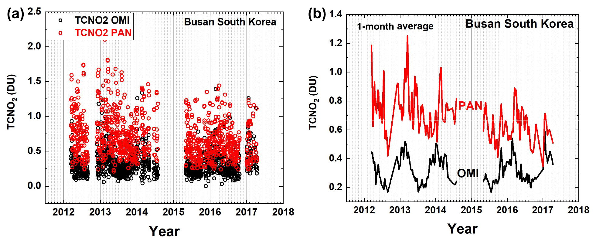
Figure 3Extended time series for Busan. (a) Individual matching PANDORA and OMI data points for the overpass time ±6 min. (b) Monthly averages.
2.2 PANDORA
PANDORA is a sun-viewing instrument for SZA < 80∘ that obtains about 4000 spectra for clear-sky views of the sun in 20 s for each of two ranges, UV (290–380 nm using a UV340 bandpass filter) and visible plus UV (280–525 nm using no filter). The overall measurement time is about 80 s, including 20 s dark-current measurements between each spectral measurement throughout the day. About 4000 clear-sky spectra for the UV and visible portions are separately averaged together to achieve very high signal-to-noise ratios (SNRs). The UV340 filter for the UV portion of the spectra reduces stray light effects from the visible wavelength range. A detailed description of PANDORA and its SNR is given in Herman et al. (2009, 2015). The effect of moderate cloud cover (reduction of the observed signal by a factor of 8) in the PANDORA FOV on TCNO2 retrievals is small (Herman et al., 2018). Cloud cover also reduces the number of measurements possible in 20 s, which potentially increases the noise level. PANDORA is driven by a highly accurate sun tracker that points an optical head at the sun and transmits the received light to an Avantes 2048×32 pixel CCD spectrometer (AvaSpec-ULS2048 from 280 to 525 nm with 0.6 nm resolution) through a 50 μm diameter fiber optic cable. The estimated TCNO2 error is approximately 0.05 DU (1 DU = 2.69×10¹⁶ molecules cm−2) out of a typical value of 0.3 DU in relatively clean areas and over 3 DU in highly polluted areas. PANDORA data are available for 250 sites. Some sites have multi-year data sets, but many of these sites are short-term campaign sites (https://avdc.gsfc.nasa.gov/pub/DSCOVR/Pandora/DATA_01/, last access: 16 July 2019).
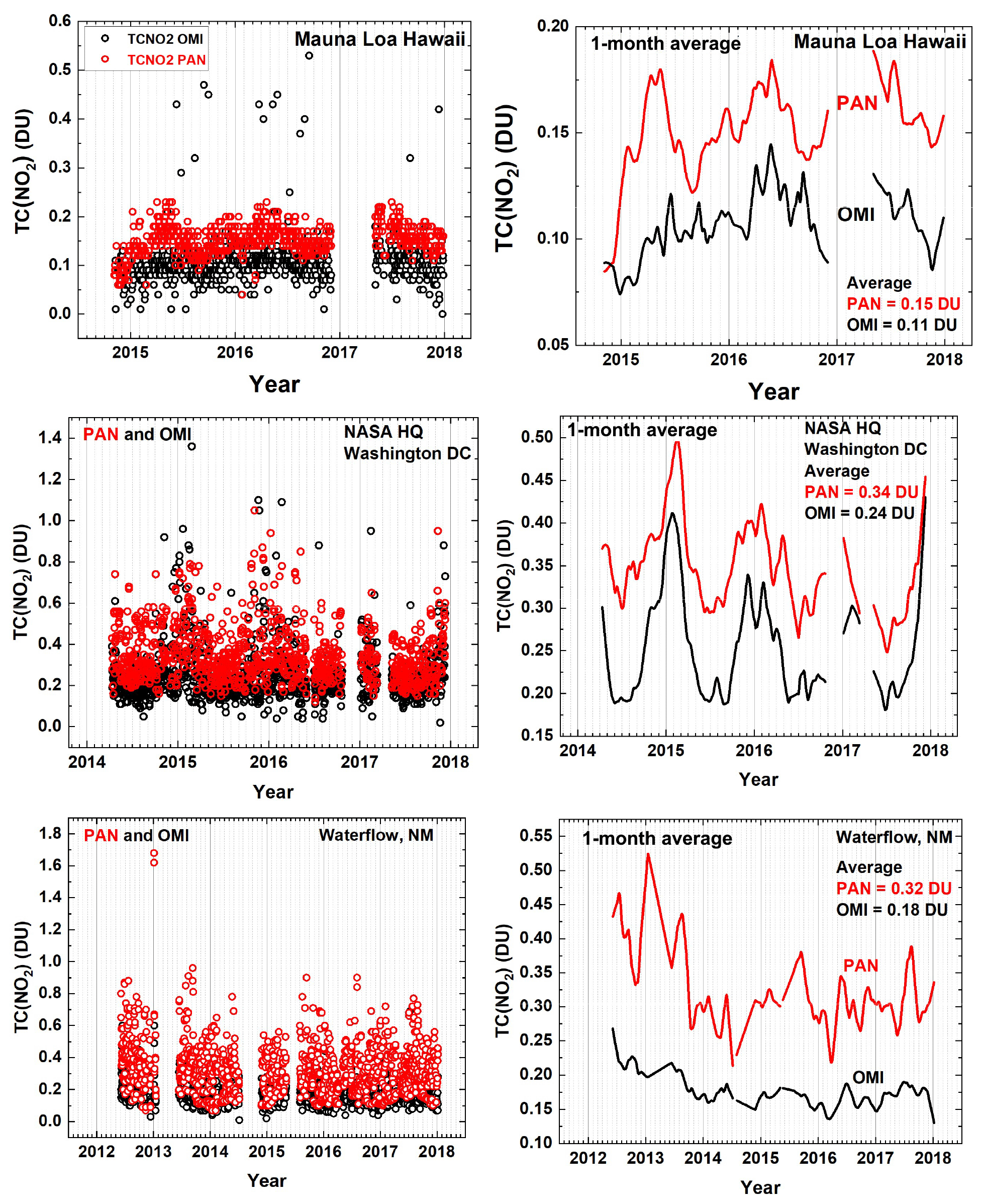
Figure 4PANDORA compared to OMI. Extended TCNO2 overpass time series for Mauna Loa Observatory, Hawaii, NASA Headquarters, Washington DC, and Waterflow, New Mexico.
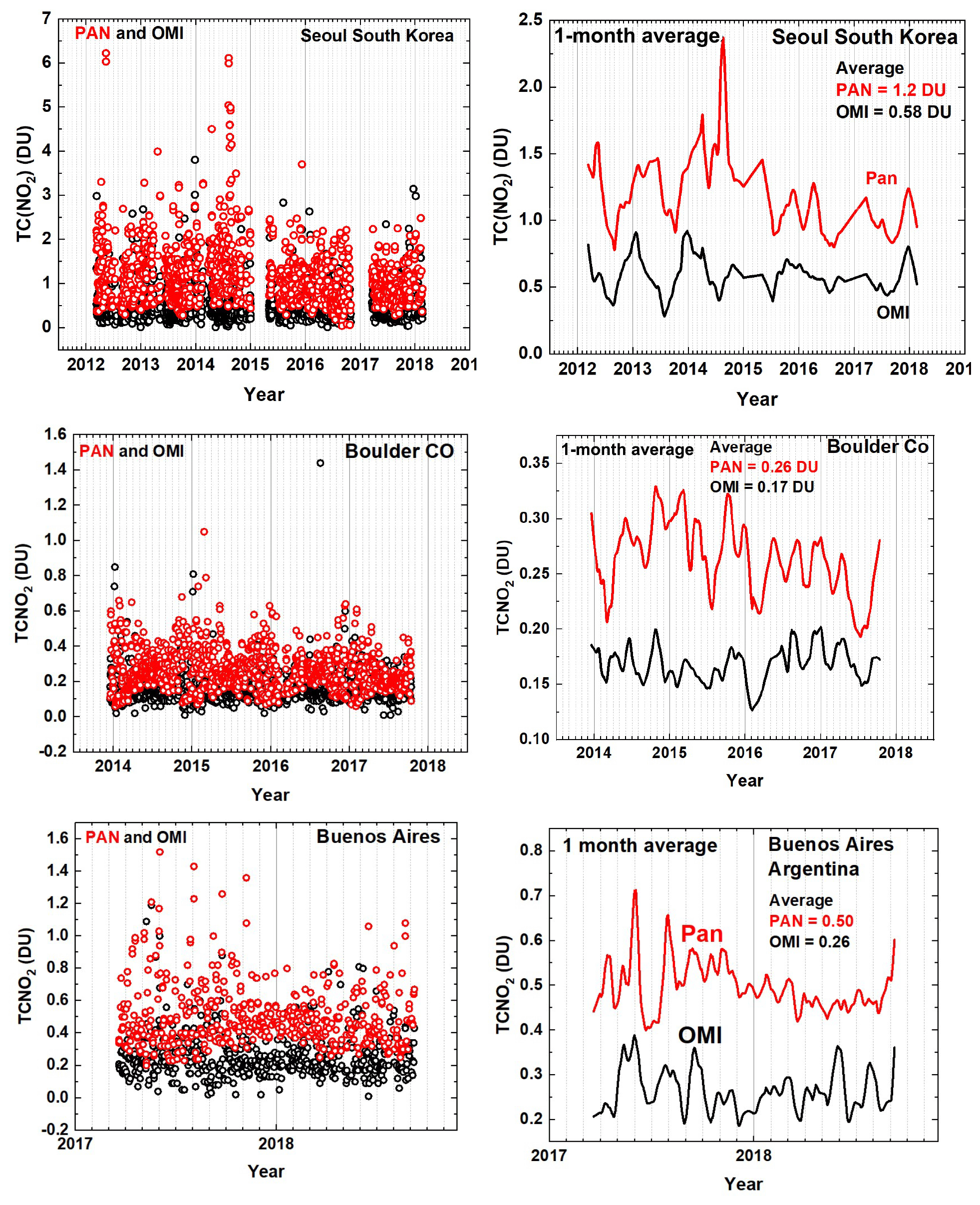
Figure 5PANDORA compared to OMI. Extended TCNO2 overpass time series for Seoul, South Korea, Boulder, Colorado, and Buenos Aires, Argentina (Raponi et al., 2018).
2.3 Overpass comparisons and diurnal variation of TCNO2
The contribution of NO2 to air quality at the earth's surface is usually a proportional function of TCNO2 that varies with the time of day and with the altitude profile shape (Lamsal et al., 2013; Bechle et al., 2013). Most of the NO2 amount is usually located between 0 and 3 km altitude with a small amount of about 0.1±0.05 DU (Dirksen et al., 2011) in the upper troposphere and stratosphere. Because of the relatively short chemical lifetime, 3–4 h (Liu et al., 2016), in the lower atmosphere, most of the NO2 is located near (0 to 20 km) its sources (industrial activity, power generation, and automobile traffic). At higher altitudes or in the winter months, the lifetime of NO2 is longer, permitting transport over larger distances from its sources.
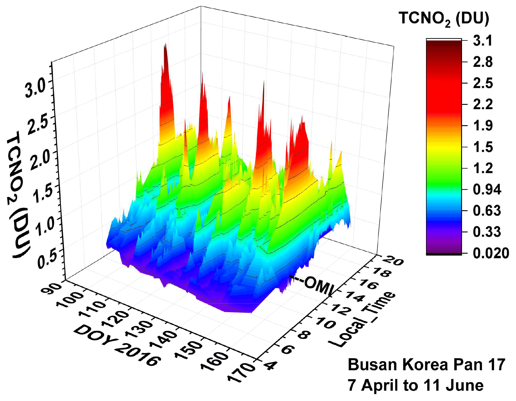
During the South Korean campaign (KORUS-AQ) in the spring of 2016 the diurnal variations of TCNO2 vs. days of the year DOY were determined for six sites (Herman et al., 2018), one of which is reproduced here (Fig. 1) for the city of Busan, showing relatively low values of TCNO2 in the morning (0.5 DU), moderately high values during the middle of the day (1.3 DU), and very high values on some of the afternoons (2 to 3 DU). Of these data, OMI only observes midday values near the 13:30 time marked on the Local_Time axis of Fig. 1, thereby missing very high values (2 to 3 DU) that frequently occur later in the afternoon coinciding with times when people are outdoors returning from work.
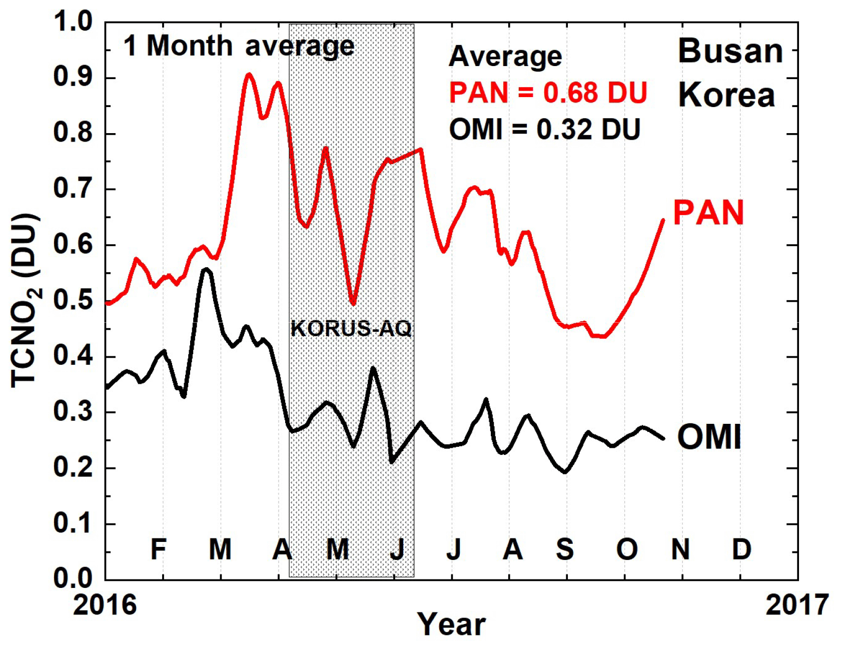
In addition to not being designed to observe the TCNO2 diurnal variation, the OMI values are about half those observed by PANDORA (Fig. 2) at the OMI overpass time, so that using OMI values to estimate NO2 pollution seriously underestimates the air quality problem even at midday. The shaded area in Fig. 2 corresponds to the period covered in the KORUS-AQ campaign of 7 April to 11 June 2016 shown in Fig. 1. An extended time series for the Busan location is shown in Fig. 3.
Because of the different effective NO2 FOV of PANDORA (measured in m2) while tracking the moving sun position located in the heart of Busan (FOV distance d<5 km for an SZA < 70∘ used for TCNO2 retrievals), both the daily (Fig. 3a) and PANDORA monthly average variations (Fig. 3b), obtained at the OMI overpass time, differ from the variation in the OMI TCNO2 caused by the much larger OMI FOV (13 km × 13 km at OMI nadir view) retrieval. Because of this, the OMI time series has low correlation (r2=0.1) with the PANDORA time series.
The extended OMI vs. PANDORA time series from 2012 to 2017 for Busan (Fig. 3) shows the same magnitude of differences seen during the KORUS-AQ period. A similar OMI vs. PANDORA plot for total column ozone TCO3 (Appendix Fig. A1) shows good agreement between PANDORA and OMI, indicating that the PANDORA instrument was operating and tracking the sun properly. Because the spatial variability of TCO3, which is mostly in the stratosphere, is much less than for TCNO2, the effect of different FOVs is minimized for ozone.
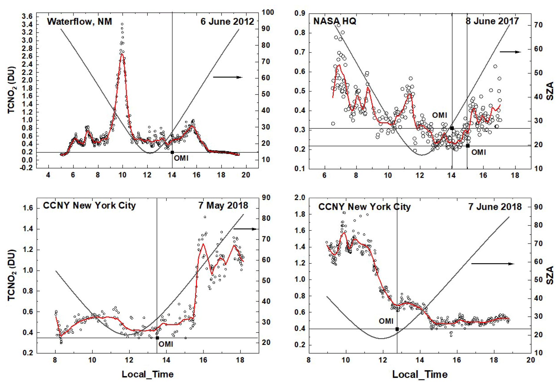
Figure 6Diurnal variation of TCNO2 on a single day (1) 2 km north of Waterflow, NM, near a power plant, (2) on the roof of NASA Headquarters in Washington DC, and (3) on the roof or a building at CCNY City College of New York, New York City.
The same type of differences, TCNO2(PAN) > TCNO2(OMI), are seen at a wide variety of sites (e.g., see Figs. 4 and 5) for Northern Hemisphere sites and one site in the Southern Hemisphere where PANDORA has an extended time series. Comparing extended Busan multi-year time series, some broad-scale correlation can be seen with peaks in February 2013, in January 2014, and in 2016. The OMI data from Busan are different than data from many sites, since Busan is located very near the ocean, causing a portion of the OMI FOV to be over the relatively unpolluted ocean areas, whereas PANDORA is located inland (Pusan University) in an area of dense automobile traffic and quite near mountains capable of trapping air.

Figure 7Percent differences between OMI and PANDORA. The slopes are the absolute change in the percent difference. For example, the Boulder percent difference goes from −31 % to −23 % over 4 years. The LS means are least squares means with the corresponding error estimates.
Figures 4 and 5 show a variety of different sites, ranging from the Mauna Loa Observatory location at 3.4 km (11 161 feet) on a relatively clean Hawaiian island surrounded by ocean to a polluted landlocked semi-arid site at Waterflow, New Mexico, near a power plant. All the sites considered show a significant underestimate of OMI TCNO2. A summary of the monthly average underestimates is given in Tables 1 and 2. For some sites there is evident correlation between the two offset measurements. For example, the PANDORA at NASA Headquarters in Washington DC tracks the OMI measurement quite well on a monthly average basis, with a correlation coefficient of r2 (mn) = 0.7, even though the daily correlation is low (r2 (d) = 0.17). Other sites have only short periods of correlation and overall weak correlation (Table 1 showing daily, d, and monthly, mn, correlation coefficients for the graphs in Figs. 4 and 5).
TCNO2(PAN) comparisons with TCNO2(OMI) from Mauna Loa Observatory MLO (Fig. 4) are not those that might be expected, since the PANDORA observations are in an area where there are almost no automobile emissions and certainly no power plants, yet PAN > OMI and TCNO2(PAN) values are large enough so that the pollution values (0.18 DU) are well above the stratospheric values (approximately 0.1 DU). OMI, which mainly measures values over the clean ocean, has an average value of about 0.1 DU (see Appendix Fig. A2). Since there are no emission or combustion sources of NO2 at high altitudes near MLO at 3.4 km, the PANDORA values suggest upward airflow from the near-sea-level circumferential ring road, Keahole oil power plant, and resort areas. The Mauna Loa TCNO2 values do not show any correlation with the recent increased volcanic activity at Mt. Kilauea after 2016. A graph showing the midday values of TCNO2 at MLO is given in the Appendix. Recently, the original Mauna Loa PANDORA was replaced. The new instrument's calibration will be reviewed before being added to the time series as part of a general data quality assurance program that starts with the most recently deployed or upgraded PANDORA instruments at about 100 locations.
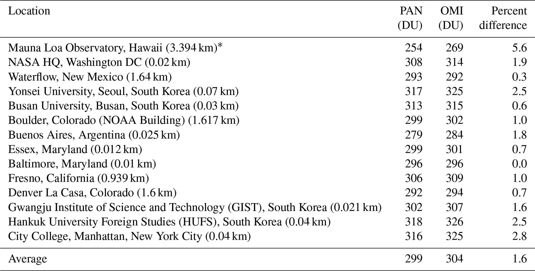
Table 1Values of TCNO2 for PANDORA and OMI from monthly averages in Figs. 4 and 5.
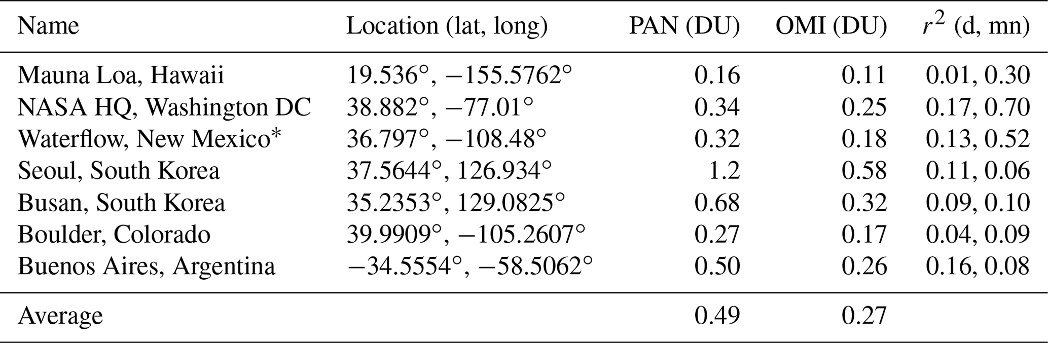
* Waterflow, NM, is listed for OMI data as Four Corners, NM, a nearby landmark.
Table 2Average values of TCNO2 for PANDORA and OMI for additional sites.
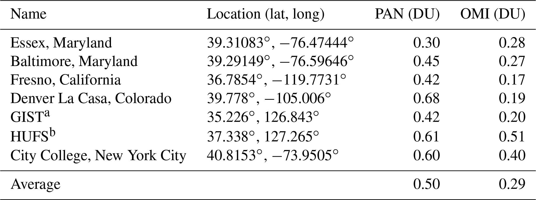
a Gwangju Institute of Science and Technology, South Korea. b Hankuk University of Foreign Studies, South Korea.
An interesting inland site is near the very small town of Waterflow, New Mexico (Figs. 4 and 6), where two power plants located near the PANDORA site ceased operation on 30 December 2013 (Lindenmaier et al., 2014). According to a quote from AZCentral Newspaper (Tuesday 31 December 2013), “Three coal-fired generators that opened in the 1960s near Farmington, N.M., closed Monday as part of a $182 million plan for Arizona Public Service Co. to meet environmental regulations, the utility reported”. The TCNO2 data suggest that the actual shutdown occurred near 15 October 2013. After the shutdown, air quality improved in the area, with TCNO2 decreasing from 0.4 to 0.28 DU. The remaining more efficient generators continued to produce smaller NO2 emissions. These were shut down at the end of 2016 with little additional observed change in TCNO2, since these boilers used NO2 scrubbers (Mavendra Dubey, personal communication, 2018; Fenton, 2015). A nearby highway (Route 64) about 2 km from the PANDORA site has little automobile traffic. An example of the diurnal behavior of TCNO2 at Waterflow, New Mexico, on 6 June 2012 is shown in Fig. 6 to illustrate the behavior of PANDORA TCNO2 retrievals at a wide range of SZAs. The terrain surrounding the Waterflow PANDORA site is flat, with no obstructions (buildings) permitting observations to very high SZAs. Almost every day the power plant briefly puts out very high emissions of NO2 as part of its daily boiler cleaning cycle. This can be seen in the very high peak value of TCNO2 of 3.4 DU compared to the nominal value of 0.5 DU occurring for most of the day. The value from the FOV-averaged OMI retrieval at 21:01 GMT (14:01 local standard time) is about 0.2 DU compared to the PANDORA value of about 0.5 DU. Figure 6 also illustrates TCNO2 diurnal behavior at two other sites, NASA HQ in Washington DC and City College of New York, and compares the values to the OMI-retrieved TCNO2.
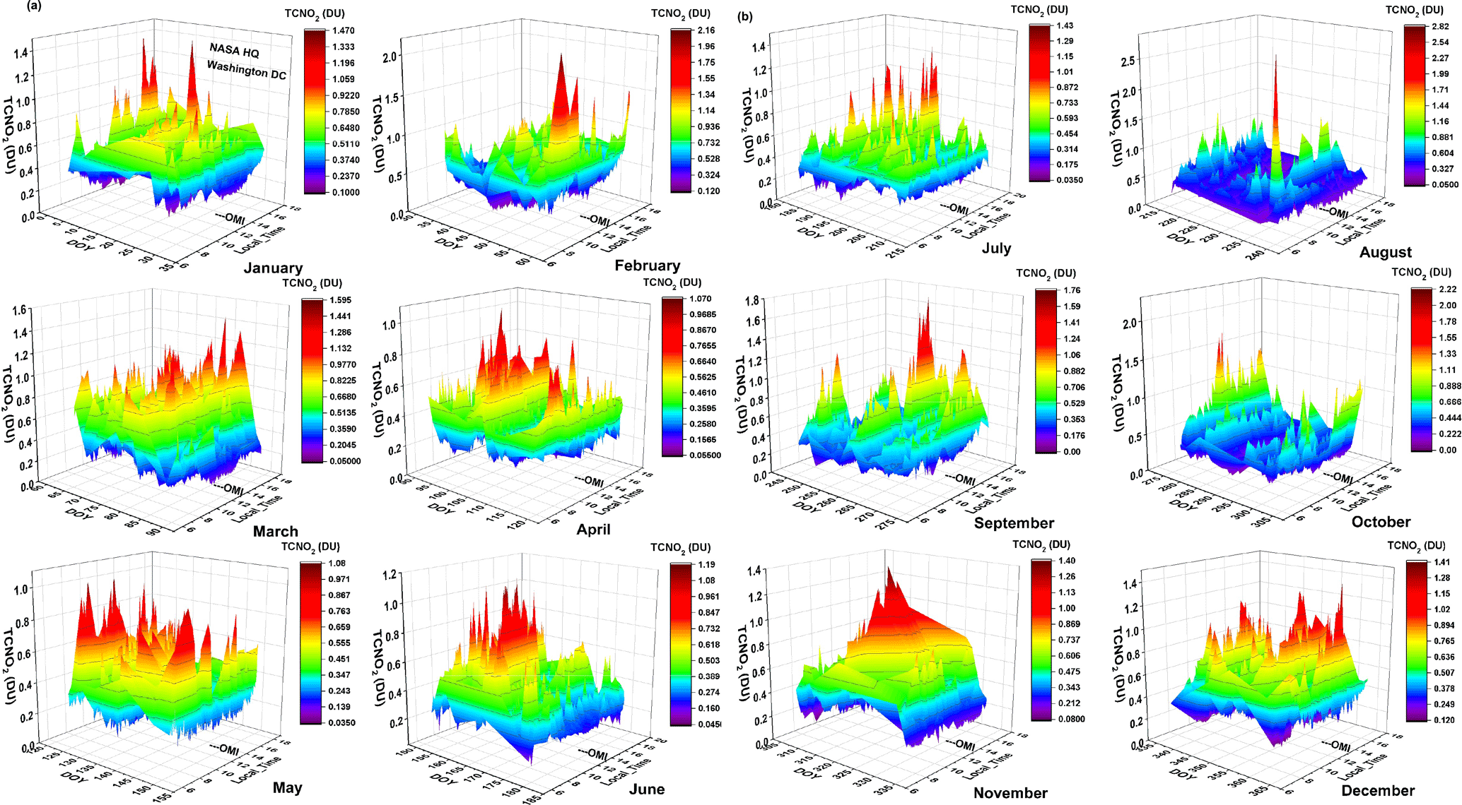
Figure 8(a) TCNO2 diurnal variation (DU) from January to June, NASA Headquarters, Washington DC, from January to June 2015. The approximate OMI overpass time near 13:30 is marked. (b) TCNO2 diurnal variation (DU) from July to December, NASA Headquarters, Washington DC, from July to December 2015. The approximate OMI overpass time near 13:30 is marked.
Both Figs. 6 and 2A show the PANDORA TCNO2 retrieval with the values of the SZA plotted on the same graph showing that the direct-sun retrievals are good out to SZA = 70∘. Depending on atmospheric conditions, retrievals using Beer's law absorption attenuation and spectral fitting for SZA > 75∘ begin to yield non-physical values (TCNO2 too small). During midday measurements, the signal-to-noise ratio is very high since over 4000 clear-sky measurements are averaged together to produce one data point every 20 s. Even with aerosol loading (no spectral features) or moderate cloud cover blocking the sun, the retrievals are still accurate (Herman et al., 2018).
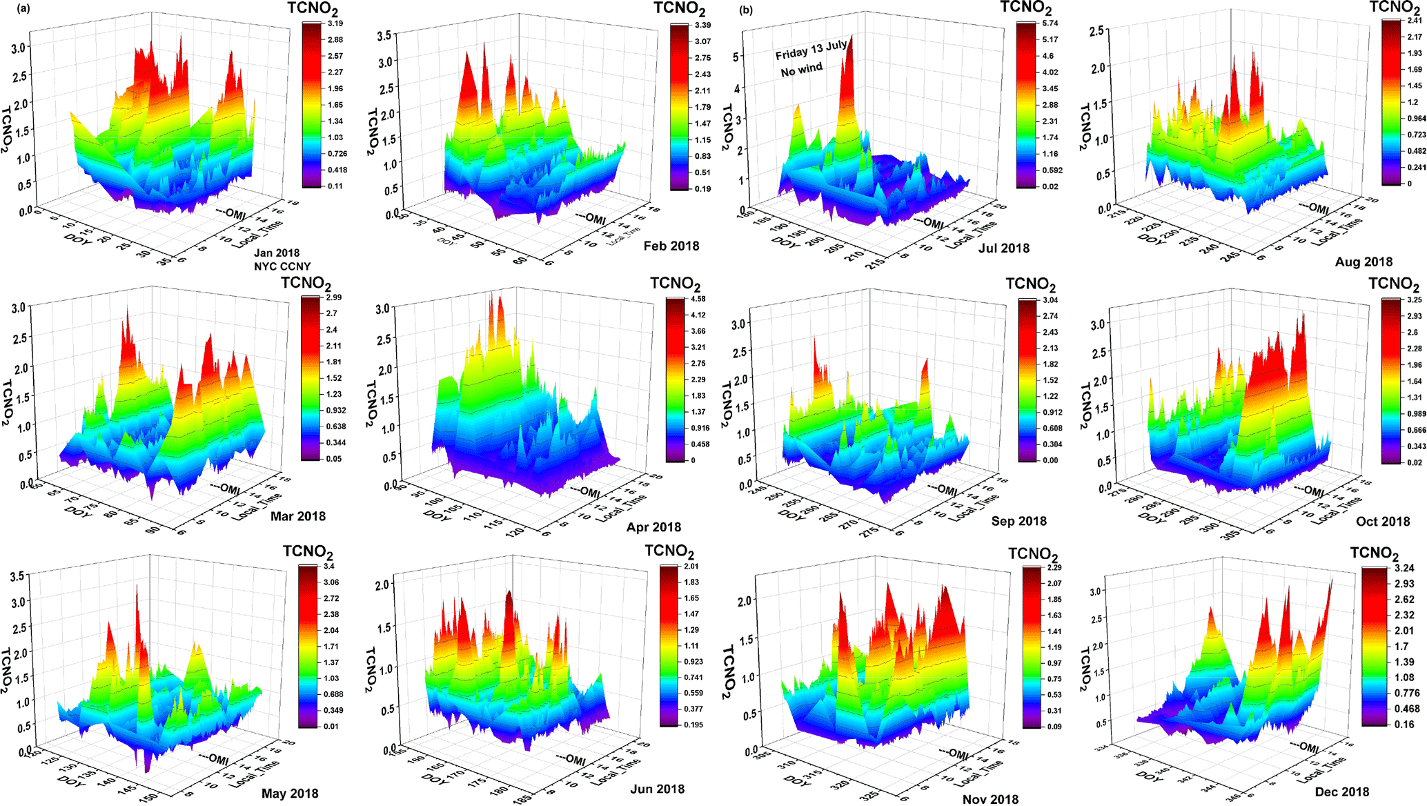
Figure 9(a) TCNO2 diurnal variation (DU) at CCNY in New York City for January to June 2018. The approximate OMI overpass time near 13:30 is marked. (b) TCNO2 diurnal variation at CCNY in New York City for July to December 2018. The peak near 5 DU occurs on 13 July 2018 between 11:20 and 12:30 EST. The approximate OMI overpass time near 13:30 is marked.
Table 2 contains a summary of some sites that were part of short-term Discover-AQ campaigns in Maryland, Texas, California, and Colorado, two longer-term sites in South Korea, and one in New York City. Essex, Maryland, is located on the Chesapeake Bay 10 km east of the center of Baltimore. The site is relatively clean (PAN = 0.3 DU) compared to the center of Baltimore (PAN = 0.45 DU), while OMI measures about the same amounts for both sites (0.28 and 0.27 DU) because the OMI FOV is larger than the distance between the two sites. The Houston, Texas, site contains 7 months of data from January to July 2013, with widespread NO2 pollution permitting PANDORA and OMI to measure the same average values even though PANDORA observes episodes on many days when TCNO2 exceeds 1.5 DU for short periods at times not observed by OMI. Observations in the small city of Fresno, California, were during January when agricultural sources of NO2 were at a minimum (Almaraz, 2018), but automobile traffic in the center of Fresno was significant. In this situation, PANDORA recorded the effect of automobile traffic, while OMI averaged the city of Fresno and surrounding fallow agricultural areas. The Denver La Casa location is in the center of the city in an area with high amounts of local automobile traffic and near the Cherokee power-generating plant. The result is a high level of average pollution (0.42 DU), while OMI measures both the city center and the surrounding relatively clean plains areas. The HUFS South Korean site is southeast of Seoul in a fairly isolated valley. However, Seoul and its surrounding areas are a widespread transported source of pollution so that both PANDORA and OMI measure elevated TCNO2 amounts. In contrast, the PANDORA Gwangju Institute of Science and Technology (GIST) site is on the outskirts of a small city in southwestern South Korea with significant traffic. The result is significant amounts of localized TCNO2 (PANDORA = 0.42) surrounded by areas that produce little NO2 leading to OMI observing a very clean 0.2 DU. The averages of sites in the two tables are similar, leading to ratios of PAN/OMI of 1.8 and 1.7, respectively. The estimated 50 % increase in OMI retrievals of TCNO2 from using the geometry-dependent reflectivity (Vasilkov et al., 2017) for the most polluted sites will narrow the disagreement with PANDORA. For example, OMI Seoul TCNO2 may become 0.87 DU (PANDORA = 1.2 DU) and Buenos Aires 0.39 DU (PANDORA = 0.5 DU), still underestimating the amount of NO2 pollution and missing the significant diurnal variation.

Figure 10TCNO2 overpass time series for CCNY in Manhattan, New York City. (a) OMI overpass TCNO2 (black) compared with OMI (red). (b) Monthly lowess (0.08) fit to the daily overpass data. (c) Percent difference 100(OMI–PAN)/PAN calculated from the data in (a).
For the six sites shown, the average OMI underestimate of TCNO2 is approximately a factor of 1.8 at the overpass time on a monthly average basis with occasional spikes that exceed this amount. The bias values range from 1.1 to 3.6, with higher biases tending to be associated with higher TCNO2 values. The factor of 1.8 underestimate ignores the frequent large values of TCNO2 at other times during the day (Fig. 7). In addition, averaging TCNO2 (PAN) over each entire day yields average values for the whole period that are 10 % to 20 % higher than just averaging over midday values that matched the OMI overpass time. Aside from the absolute magnitude, the short-term variations (over several months) are similar for both OMI and PANDORA although mostly not correlated. If correlation coefficients r2 are generated from linear fits to scatter plots of TCNO2 from OMI vs. PANDORA, the correlation is mostly poor (examples: r2=: Seoul 0.06, Mauna Loa 0.3, and NASA HQ 0.7; see Figs. 4 and 5). Additional sites with shorter PANDORA time series of TCNO2 show similar behavior.
Duncan et al. (2016) estimated trends from OMI TCNO2 time series and found that the Seoul metropolitan area had a decrease of % yr−1 (2005–2014) consistent with an OMI-estimated change of % yr−1 (2012–2018) in this paper. However, for the small area near Yonsei University, the decrease estimated from PANDORA is % yr−1. Park (2019) estimates that metropolitan Seoul has decreased in population even as surrounding areas have increased in population.
The average percent differences between OMI and PANDORA shown in Fig. 7 are relatively constant over time for each site, with small changes over each multi-year observation period. The differences between OMI and PANDORA are provided by forming the percent differences of the daily TCNO2 values (Fig. 7) in the form 100(OMI–PAN)/PAN. Also shown are the average percent differences and the linear fit slopes in percent change per year of the percent differences over the multi-year period. For example, the Boulder percent difference goes from −31 % to −23 % over 4 years. Of the six sites in shown in Fig. 7, two have statistically significant slopes, Seoul, South Korea (2.1±0.5 % yr−1) and NASA Headquarters in Washington DC (3.4±0.9 % yr−1), at the 2σ level, suggesting a significant area average increase in pollution compared to PANDORA's local values.
For some sites (see Fig. 7), PANDORA and OMI trends are the same within statistical uncertainty (Waterflow, NM, Buenos Aires, and Mauna Loa), while the other three sites show significantly different trends (Boulder, NASA HQ, and Seoul).
The results for Busan (from Fig. 3) show a least squares average for the percent difference of % for the 2012–2018 period with a slope of 6.8±1 % yr−1. There is a decrease in the percent difference after October 2015 (Fig. 3) that is mainly from PANDORA seeing less TCNO2 than during the 2012–2014 period. There is a gap in the Busan time series from July 2014 until April 2015, when the original PANDORA was replaced with a new instrument. The calibrations of both PANDORAs appear to be correct. Because of the break in the time series it is not clear whether there was a change in local conditions around Pusan University compared to the wide area observed by OMI.
2.4 Diurnal variation of TCNO2 compared to OMI retrievals
Figure 8 shows details of the daily diurnal variation of TCNO2 on the roof of NASA Headquarters, Washington DC, adjacent to a major cross-town highway (I695) for every day during each month of 2015 for local time vs. DOY. The midday observing local standard time for OMI is marked for each graph. Displaying an entire year of daily (2 min time resolution) PANDORA data shows that the high values of TCNO2 are a frequent occurrence but do not occur every day.
The amount of TCNO2 is mostly from the adjacent highway and the surrounding urban area with heavy traffic. The relatively moderate TCNO2 values (0.4 to 0.8 DU) are probably a testament to the effectiveness of catalytic converters mandatory on all US automobiles in such a high traffic area (Bishop and Steadman, 2015). The same data are plotted in Fig. 6 for 8 June 2017, showing that OMI reasonably matched the values seen by PANDORA at 14:00 and 15:00 but was not available to observe high values that occurred in the morning.
Figure 9 contains the daily TCNO2 diurnal variability vs. DOY for each month measured by a PANDORA from the roof of a building on the CCNY (City College of New York) campus in the middle of Manhattan in New York City (NYC). From the values shown, the pollution levels are quite high, rivaling the pollution levels in Seoul, South Korea (see Fig. 5). OMI at its midday overpass time would detect some of the high-level pollution events but miss many others occurring mostly in the afternoon. There are a significant number of days in all the months where the TCNO2 levels appear to be low (e.g., blue color in July and October), but the blue color still represents significant pollution levels (TCNO2(PAN) > 0.5 DU) that are small only compared to the peak values during the month (TCNO2(PAN) > 1 DU). The highest amount of TCNO2 recorded during 2018 was about 5 DU on 13 July 2018 from 11:20 and 12:30 EST, a time with very light winds (1 km h−1) and moderate temperature (25 ∘C). There were many smaller peaks between 2 and 3 DU throughout the year. Extreme cases of high NO2 amounts are frequently associated with the local meteorology indications of stagnant air (Harkey et al., 2015). The same data are shown in Fig. 6 for two days, 7 May and 7 June 2018, showing the comparison with OMI and the occurrence of much higher values of TCNO2 in the morning and afternoon.
For both Washington DC (Fig. 8) and New York City (Fig. 9) there is strong day-to-day and month-to-month variability that depends on the local meteorological conditions (Seo et al., 2018; Zheng et al., 2015) and the amount of automobile traffic in the area (Andersen et al., 2011; Amin et al., 2017). High TCNO2 events occur most often in the afternoon such that the OMI overpass near 13:30 would miss most high TCNO2 events. Poor air quality affecting respiratory health would be improperly characterized by both the OMI average values being too low (Fig. 4) and by missing the extreme pollution events that occur frequently in the late afternoon. The high value of TCNO2 that occurred on 5 August (2.2 DU) at 07:45 EST for Washington DC is not a retrieval error (SZA less than 70∘), but is a one-time anomaly in 2015 compared to more usual high values of 1.5 DU with an occasional spike to 2 DU. It should be noted that TCNO2 does not accurately represent the NO2 concentration at the surface, since it is mostly a measure of the amount in the lower 2 km. However, it is roughly proportional to the surface measurements close to the pollution sources (Bechle et al., 2013; Knepp et al., 2014), with the exact proportionality dependent on the profile shape near the ground.
Similar daily diurnal variation graphs of TCNO2 (Figs. 8 and 9) could be shown for each site. However, the basic idea is the same for each site. OMI underestimates the amount of TCNO2 because of its large FOV and misses most of the peak events at other times of the day. For some sites, such as Busan and Seoul, the peak values can reach 3 DU and above late in the afternoon, which are never seen by OMI (Herman et al., 2018).
Figure 10 for CCNY is similar to the graphs in Figs. 4–6 showing the relative behavior between PANDORA and OMI but including only OMI pixels that are at a distance D < 30 km from CCNY. The results are almost identical to those when D < 80 km. There is a period in March 2018 when OMI TCNO2 slightly exceeded that measured by PANDORA. OMI with its large FOV may be seeing part of the chemically driven seasonal variation, while PANDORA is seeing a nearly constant source driven amount mostly from automobile traffic. For most days during 2018, PAN(TCNO2) > OMI(TCNO2), with the average value for PAN = 0.65 DU and for OMI = 0.45 DU (Fig. 10b). The percent difference plot shows that there is a systematic increase between PANDORA and OMI TCNO2 from a value of 10 % to a value of 50 %.
Examination of long-term TCNO2 monthly average time series from the OMI satellite and PANDORA ground-based observations shows that OMI systematically underestimates the amount of NO2 in the atmosphere by an average factor of 1.5 to 2 at the local OMI overpass time near the Equator crossing time of 13:30 ± 01:30. As shown in Fig. 7 for TCNO2, 100(OMI–PAN)/PAN least squares mean underestimates are much larger than error estimates. These differences are reduced for the smaller pixel size TropOMI TCNO2 values (Judd et al., 2019). In addition, the PANDORA diurnal time series for every day during a year at each site (only two typical sites are shown in this paper, NYC and NASA-HQ) shows peaks in TCNO2 that are completely missed by only observing at midday (see Figs. 6, 8, 9, and A2). The result is that estimates of air quality related to health effects from OMI observations are strongly underestimated almost everywhere, as shown at all the sites with a long PANDORA record. In comparisons to PANDORA, OMI data are mostly uncorrelated or weakly correlated (e.g., Seoul correlation coefficient r2=0.06, Mauna Loa r2=0.3), while NASA HQ in Washington DC shows a correlation on a seasonal basis (NASA HQ r2=0.7), suggesting a wide area coordinated source of NO2 (most likely automobile traffic). The data from CCNY show some correlation between the locations of the peaks and troughs. Seven short-term TCNO2 time series were examined, showing similar results (Table 1), except when the pollution region is widespread as in the Seoul, South Korea, region. The conclusion is that while OMI satellite TCNO2 data are uniquely able to assess regional long-term trends in TCNO2 and provide a measure of the regional distribution of pollutants, the OMI data cannot properly assess local air quality or the effect on human health over extended periods in urban or industrial areas. This will continue to be the case, but to a lesser degree, when the OMI TCNO2 data are improved by reprocessing with a new geometry-dependent reflectivity (Vasilkov et al., 2017) and by the smaller FOV of TropOMI. The analysis shows that locating PANDORAs at polluted sites could provide quantitative corrections for spatial and temporal biases that affect the determination of local air quality from satellite data. Satellite detection of diurnal variation of TCNO2 will be improved with the upcoming launch of three planned geostationary satellites over Korea, the US, and Europe to verify the proper operation of the various PANDORA instruments. A similar analysis for total column ozone (TCO) was performed (see Appendix) and shows close agreement between OMI and PANDORA, with the largest difference occurring for Mauna Loa Observatory at 3.4 km altitude, where PANDORA misses the ozone between the surface and 3.4 km.
The data used in this paper can be accessed from a NASA website Pandora Data on https://avdc.gsfc.nasa.gov/pub/DSCOVR/Pandora/DATA/ (last access: 15 October 2019) and OMI Data on https://avdc.gsfc.nasa.gov/index.php?site=666843934&id=13 (last access: 15 October 2019).
Ozone: this section shows the corresponding PANDORA total column ozone (TCO) values compared to OMI TCO for Busan, South Korea (Fig. A1), that shows close agreement for the entire 2012–2017 period. The different fields of view for OMI and PANDORA have a much smaller effect because of the greater spatial uniformity of stratospheric ozone compared to tropospheric NO2. Additional sites are summarized in Table A1. The largest TCO difference (15 DU or 5.6 %) occurs for Mauna Loa Observatory (altitude = 3.4 km) compared to OMI (average altitude = sea level). The close results show that the PANDORA was working properly and pointing accurately at the sun. The PANDORA TCO data shown here use a mid-latitude effective ozone temperature correction from model calculations that may not be accurate for each individual site (Herman et al., 2017). The ozone retrievals shown here use an average effective ozone temperature instead of a locally measured ozone temperature (Herman et al., 2015, 2017).
Table A1Average values of TCO3 for PANDORA and OMI.
* Mauna Loa TCNO2: Fig. A2 shows the diurnal variation of TCNO2 at MLO on specific days 3, 4, 7, and 8 June 2016 along with the variation in SZA. This shows that the MLO is polluted by NO2 with column amounts in excess of stratospheric amounts (approximately 0.1 DU) even though there are no local sources. OMI retrievals of TCNO2 on each day are much lower (about 0.12 DU) because of the averaging over OMI's large FOV that includes very clean ocean areas.
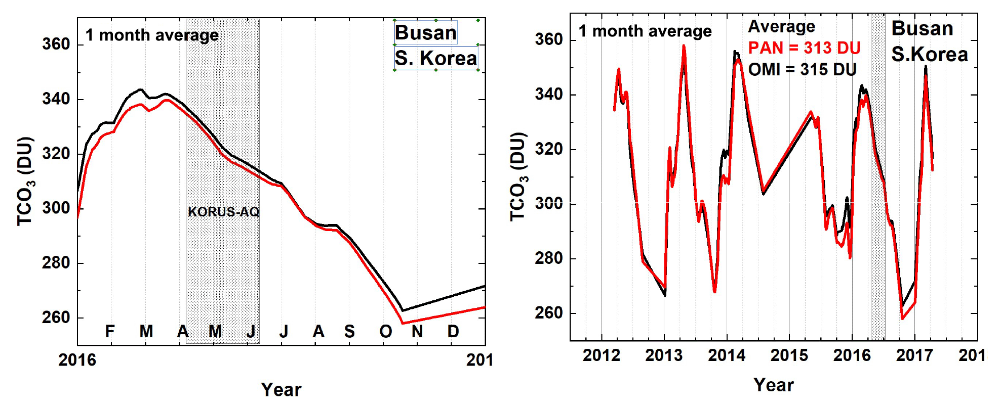
Figure A1Monthly average values of TCO for OMI and PANDORA at OMI overpass times for Busan, South Korea. Shaded area represents the KORUS-AQ campaign period.
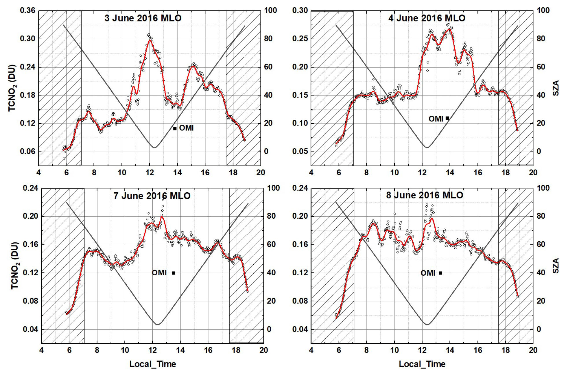
Figure A2The diurnal variation of TCNO2 at MLO on 4 d during June 2016 compared to OMI TCNO2 (small square). Shaded areas represent high SZA conditions where the PANDORA retrievals are not accurate.
JH produced all of the figures and text, JhK and JaK contributed the Korean PANDORA data, MD contributed the data from Waterflow, New Mexico, and the CO2 analysis, MR contributed the Buenos Aires PANDORA data, and MT contributed the PANDORA data from CCNY.
The authors declare that they have no conflict of interest.
This project is supported by the Korean Ministry of Environment (MOE) as a Public Technology Program based on Environmental Policy (2017000160001), by the Los Alamos National Laboratory's Laboratory Directed Research and Development program, and by the NASA PANDORA project managed by Robert Swap.
This research has been supported by the NASA PANDORA project supported by the NASA Tropospheric Composition Program.
This paper was edited by Folkert Boersma and reviewed by two anonymous referees.
Almaraz, M., Bai, E., Wang, C., Trousdel, J., Conley, S., Faloona, I., and Houlton, B. Z.: Agriculture is a major source of NOx pollution in California, Sci. Adv., 31, 1–8, https://doi.org/10.1126/sciadv.aao3477, 2018.
Amin, S. R., Tamima, U., and Jimenez, L. A.: Understanding Air Pollution from Induced Traffic during and after the Construction of a New Highway: Case Study of Highway 25 in Montreal, J. Adv. Transport., 2017, 5161308, https://doi.org/10.1155/2017/5161308, 2017.
Andersen, Z. J., Hvidberg, M., Jensen, S. S., Ketzel, M., Loft, S., Sørensen, M., Tjønneland, A., Overvad, K., and Raaschou-Nielsen, O.: Chronic obstructive pulmonary disease and long-term exposure to traffic-related air pollution: A cohort study, Am. J. Respir. Crit. Care Med., 183, 455–461, https://doi.org/10.1164/rccm.201006-0937OC, 2011.
Bechle, M. J., Millet, D. B., and Marshall, J. D.: Remote sensing of exposure to NO2: Satellite versus ground-based measurement in a large urban area, Atmos. Environ., 69, 345–353, 2013.
Bishop, G. A. and Stedman, D. H.: Reactive Nitrogen Species Emission Trends in Three Light-/Medium-Duty United States Fleets, Environ. Sci. Technol., 49, 11234–11240, https://doi.org/10.1021/acs.est.5b02392, 2015.
Boersma, K. F., Eskes, H. J., and Brinksma, E. J.: Error analysis for tropospheric NO2 retrieval from space, J. Geophys. Res.-Atmos., 1–20, https://doi.org/10.1029/2003JD003962, 2004.
Boersma, K. F., Eskes, H. J., Dirksen, R. J., van der A, R. J., Veefkind, J. P., Stammes, P., Huijnen, V., Kleipool, Q. L., Sneep, M., Claas, J., Leitão, J., Richter, A., Zhou, Y., and Brunner, D.: An improved tropospheric NO2 column retrieval algorithm for the Ozone Monitoring Instrument, Atmos. Meas. Tech., 4, 1905–1928, https://doi.org/10.5194/amt-4-1905-2011, 2011.
Boersma, K. F., Vinken, G. C. M., and Eskes, H. J.: Representativeness errors in comparing chemistry transport and chemistry climate models with satellite UV–Vis tropospheric column retrievals, Geosci. Model Dev., 9, 875–898, https://doi.org/10.5194/gmd-9-875-2016, 2016.
Choudhari, S. K., Chaudhary, M., Bagde, S., Gadbai, A. R., and Joshi, V.: Nitric oxide and cancer: a review, W. J. Surg. Oncol., 11, 118, 2013.
Cleveland, W. S.: LOWESS: A program for smoothing scatterplots by robust locally weighted regression, The American Statistician, JSTOR, 35, 54, https://doi.org/10.2307/2683591, 1981.
Dirksen, R. J., Boersma, K. F., Eskes, H. J., Ionov, D. V., Bucsela, E. J., Levelt, P. F., and Kelder, H. M.: Evaluation of stratospheric NO2 retrieved from the Ozone Monitoring Instrument: Intercomparison, diurnal cycle, and trending, J. Geophys. Res., 116, 1–22, https://doi.org/10.1029/2010JD014943, 2011.
Duncan, B. N., Lamsal, L. N., Thompson, A. M., Yoshida, Y., Lu, Z., Streets, D. G., Hurwitz, M. M., and Pickering, K. E.: A space-based, high-resolution view of notable changes in urban NOx pollution around the world (2005–2014), J. Geophys. Res.-Atmos.,121, 976–996, https://doi.org/10.1002/2015JD024121, 2016.
Fenton, J.: Power plants install emissions controls, Farmington Daily Times, available at: http://www.daily-times.com/story/news/local/four-corners/2015/10/12/power-plants-install-emissions-controls/73823014/ (last access: 13 October 2015), 2015.
Goldberg, D. L., Saide, P. E., Lamsal, L. N., de Foy, B., Lu, Z., Woo, J.-H., Kim, Y., Kim, J., Gao, M., Carmichael, G., and Streets, D. G.: A top-down assessment using OMI NO2 suggests an underestimate in the NOx emissions inventory in Seoul, South Korea, during KORUS-AQ, Atmos. Chem. Phys., 19, 1801–1818, https://doi.org/10.5194/acp-19-1801-2019, 2019.
Harkey, M., Holloway, T., Oberman, J., and Scotty, E.: An evaluation of CMAQ NO2 using observed chemistry-meteorology correlations, J. Geophys. Res.-Atmos., 120, 11775–11797, https://doi.org/10.1002/2015JD023316, 2015.
Herman, J., Cede, A., Spinei, E., Mount, G., Tzortziou, M., and Abuhassan, N.: NO2 column amounts from ground-based Pandora and MFDOAS spectrometers using the direct-sun DOAS technique: Intercomparisons and application to OMI validation, J. Geophys. Res., 114, D13307, https://doi.org/10.1029/2009JD011848, 2009.
Herman, J., Evans, R., Cede, A., Abuhassan, N., Petropavlovskikh, I., and McConville, G.: Comparison of ozone retrievals from the Pandora spectrometer system and Dobson spectrophotometer in Boulder, Colorado, Atmos. Meas. Tech., 8, 3407–3418, https://doi.org/10.5194/amt-8-3407-2015, 2015.
Herman, J., Evans, R., Cede, A., Abuhassan, N., Petropavlovskikh, I., McConville, G., Miyagawa, K., and Noirot, B.: Ozone comparison between Pandora #34, Dobson #061, OMI, and OMPS in Boulder, Colorado, for the period December 2013–December 2016, Atmos. Meas. Tech., 10, 3539–3545, https://doi.org/10.5194/amt-10-3539-2017, 2017.
Herman, J., Spinei, E., Fried, A., Kim, J., Kim, J., Kim, W., Cede, A., Abuhassan, N., and Segal-Rozenhaimer, M.: NO2 and HCHO measurements in Korea from 2012 to 2016 from Pandora spectrometer instruments compared with OMI retrievals and with aircraft measurements during the KORUS-AQ campaign, Atmos. Meas. Tech., 11, 4583–4603, https://doi.org/10.5194/amt-11-4583-2018, 2018.
Ialongo, I., Herman, J., Krotkov, N., Lamsal, L., Boersma, K. F., Hovila, J., and Tamminen, J.: Comparison of OMI NO2 observations and their seasonal and weekly cycles with ground-based measurements in Helsinki, Atmos. Meas. Tech., 9, 5203–5212, https://doi.org/10.5194/amt-9-5203-2016, 2016.
Judd, L. M., Al-Saadi, J. A., Valin, L. C., Pierce, R. B., Yang, K., Janz, S. J., Kowalewski, M. G., Szykman, J. J., Tiefengraber, M., and Mueller, M.: The Dawn of Geostationary Air Quality Monitoring: Case Studies From Seoul and Los Angeles, Environ. Sci., 1–17,https://doi.org/10.3389/fenvs.2018.00085, 2018.
Judd, L. M., Al-Saadi, J. A., Janz, S. J., Kowalewski, M. G., Pierce, R. B., Szykman, J. J., Valin, L. C., Swap, R., Cede, A., Mueller, M., Tiefengraber, M., Abuhassan, N., and Williams, D.: Evaluating the impact of spatial resolution on tropospheric NO2 column comparisons within urban areas using high-resolution airborne data, Atmos. Meas. Tech. Discuss., https://doi.org/10.5194/amt-2019-161, in review, 2019.
Kim, S.-Y. and Song, I.: National-scale exposure prediction for long-term concentrations of particulate matter and nitrogen dioxide in South Korea, Environ. Pollut., 226, 21–29, https://doi.org/10.1016/j.envpol.2017.03.056, 2017.
Kleipool, Q. L., Dobber, M. R., De Haan, J. F., and Levelt, P. F.: Earth Surface Reflectance Climatology from Three Years of OMI Data, J. Geophys. Res., 113, 1–22, https://doi.org/10.1029/2008JD010290, 2008.
Knepp, T., Pippin, M., Crawford, J., Szykman, J., Long, R., Cowen, L., Cede, A., Abuhassan, N., Herman, J., Delgado, R., Compton, J., Berkoff, T., Fishman, J., Martins, D., Stauffer, R., Thompson, A., Weinheimer, A., Knapp, D., Montzka, D., Lenschow, D., and Neil, D.: Estimating Surface NO2 and SO2 Mixing Ratios from Fast-Response Total Column Observations and Potential Application to Geostationary Missions, J. Atmos. Chem., Springer, New York, NY, 1–26, 2014.
Kollonige, D. E., Thompson, A. M., Josipovic, M., Tzortziou, M., Beukes, J. P., Burger, R., Martins, D. K., van Zyl, P. G., Vakkari, V., and Laakso, L.: OMI satellite and ground-based Pandora observations and their application to surface NO2 estimations at terrestrial and marine sites, J. Geophys. Res.-Atmos., 123, 1441–1459, https://doi.org/10.1002/2017JD026518, 2018.
Krotkov, N. A., Lamsal, L. N., Celarier, E. A., Swartz, W. H., Marchenko, S. V., Bucsela, E. J., Chan, K. L., Wenig, M., and Zara, M.: The version 3 OMI NO2 standard product, Atmos. Meas. Tech., 10, 3133–3149, https://doi.org/10.5194/amt-10-3133-2017, 2017.
Lamsal, L., Randall, M., Parrish, D., and Krotkov, N.: Scaling Relationship for NO2 Pollution and Urban Population Size: A Satellite Perspective, Environ. Sci. Technol., 47, 12707–12716, https://doi.org/10.1021/es400744g, 2013.
Lamsal, L. N., Krotkov, N. A., Celarier, E. A., Swartz, W. H., Pickering, K. E., Bucsela, E. J., Gleason, J. F., Martin, R. V., Philip, S., Irie, H., Cede, A., Herman, J., Weinheimer, A., Szykman, J. J., and Knepp, T. N.: Evaluation of OMI operational standard NO2 column retrievals using in situ and surface-based NO2 observations, Atmos. Chem. Phys., 14, 11587–11609, https://doi.org/10.5194/acp-14-11587-2014, 2014.
Lamsal, L. N., Janz, S. J., Krotkov, N. A., Pickering, K. E., Spurr, R. J. D., Kowalewski, M. G., Loughner, C. P., Crawford, J. H., Swartz, W. H., and Herman, J. R.: High-resolution NO2 observations from the Airborne Compact Atmospheric Mapper Retrieval and validation, J. Geophys. Res.-Atmos., 122, 1953–1970, https://doi.org/10.1002/2016JD025483, 2017.
Levelt, P. F., Van den Oord, G. H. J., Dobber, M. R., Malkki, A., Visser, H., de Vries, J., Stammes, P., Lundell, J. O. V., and Saari, H.: The Ozone Monitoring Instrument, IEEE T. Geosci. Remote, 44, 1093–1101, https://doi.org/10.1109/tgrs.2006.872333, 2006.
Lin, J.-T., Martin, R. V., Boersma, K. F., Sneep, M., Stammes, P., Spurr, R., Wang, P., Van Roozendael, M., Clémer, K., and Irie, H.: Retrieving tropospheric nitrogen dioxide from the Ozone Monitoring Instrument: effects of aerosols, surface reflectance anisotropy, and vertical profile of nitrogen dioxide, Atmos. Chem. Phys., 14, 1441–1461, https://doi.org/10.5194/acp-14-1441-2014, 2014.
Lindenmaier, R., Dubey, M. K., Henderson, B. G., Butterfield, Z. T., Herman, J. R., Rahn, T., and Lee, S.-H.: Multiscale observations of CO2, (CO2)-C-13, and pollutants at Four Corners for emission verification and attribution, P. Natl. Acad. Sci. USA, 111, 8386–8391, https://doi.org/10.1073/pnas.1321883111, 2014.
Liu, F., Beirle, S., Zhang, Q., Dörner, S., He, K., and Wagner, T.: NOx lifetimes and emissions of cities and power plants in polluted background estimated by satellite observations, Atmos. Chem. Phys., 16, 5283–5298, https://doi.org/10.5194/acp-16-5283-2016, 2016.
Lorente, A., Boersma, K. F., Stammes, P., Tilstra, L. G., Richter, A., Yu, H., Kharbouche, S., and Muller, J.-P.: The importance of surface reflectance anisotropy for cloud and NO2 retrievals from GOME-2 and OMI, Atmos. Meas. Tech., 11, 4509–4529, https://doi.org/10.5194/amt-11-4509-2018, 2018.
Marchenko, S., Krotkov, N. A., Lamsal, L. N., Celarier, E. A., Swartz, W. H., and Bucsela, E. J.: Revising the slant column densityretrieval of nitrogen dioxide observed by the Ozone Monitoring Instrument, J. Geophys. Res.-Atmos., 120, 5670–5692, https://doi.org/10.1002/2014JD022913, 2015.
Nowlan, C. R., Liu, X., Leitch, J. W., Chance, K., González Abad, G., Liu, C., Zoogman, P., Cole, J., Delker, T., Good, W., Murcray, F., Ruppert, L., Soo, D., Follette-Cook, M. B., Janz, S. J., Kowalewski, M. G., Loughner, C. P., Pickering, K. E., Herman, J. R., Beaver, M. R., Long, R. W., Szykman, J. J., Judd, L. M., Kelley, P., Luke, W. T., Ren, X., and Al-Saadi, J. A.: Nitrogen dioxide observations from the Geostationary Trace gas and Aerosol Sensor Optimization (GeoTASO) airborne instrument: Retrieval algorithm and measurements during DISCOVER-AQ Texas 2013, Atmos. Meas. Tech., 9, 2647–2668, https://doi.org/10.5194/amt-9-2647-2016, 2016.
O'Byrne, G., Martin, R. V., van Donkelaar, A., Joiner, J., and Celarier, E. A.: Surface reflectivity from the Ozone Monitoring Instrument using the Moderate Resolution Imaging Spectroradiometer to eliminate clouds: Effects of snow on ultraviolet and visible trace gas retrievals, J. Geophys. Res., 115, D17305, https://doi.org/10.1029/2009JD013079, 2010.
Park, S. H.: Seoul, The Wiley Blackwell Encyclopedia of Urban and Regional Studies, edited by: Orum, A., John Wiley & Sons Ltd., Hoboken, https://doi.org/10.1002/9781118568446.eurs0283, 2019.
Raponi, M. M., Cede, A., Santana Diaz, D., Sánchez, R., Otero, L. A., Salvador, J. O., Ristori, P. R., and Quel, E. J.: Total Column Ozone Measured In Buenos Aires Between March And November 2017, Using A Pandora Spectrometer System, Anales AFA, 29, 46–50, https://doi.org/10.31527/analesafa.2018.29.2.46, 2018.
Seo, J., Park, D.-S. R., Kim, J. Y., Youn, D., Lim, Y. B., and Kim, Y.: Effects of meteorology and emissions on urban air quality: a quantitative statistical approach to long-term records (1999–2016) in Seoul, South Korea, Atmos. Chem. Phys., 18, 16121–16137, https://doi.org/10.5194/acp-18-16121-2018, 2018.
Strahan, S. E., Duncan, B. N., and Hoor, P.: Observationally derived transport diagnostics for the lowermost stratosphere and their application to the GMI chemistry and transport model, Atmos. Chem. Phys., 7, 2435–2445, https://doi.org/10.5194/acp-7-2435-2007, 2007.
Torres, O., Bhartia, P. K., Jethva, H., and Ahn, C.: Impact of the ozone monitoring instrument row anomaly on the long-term record of aerosol products, Atmos. Meas. Tech., 11, 2701–2715, https://doi.org/10.5194/amt-11-2701-2018, 2018.
Tzortziou, M., Parker, O., Lamb, B., Herman, J. R., Lamsal, L., Stauffer, R., and Abuhassan, N.: Atmospheric Trace Gas (NO2 and O3) Variability in South Korean Coastal Waters, and Implications for Remote Sensing of Coastal Ocean Color Dynamics, Remote Sens., 10, 1587, https://doi.org/10.3390/rs10101587, 2018.
Vasilkov, A., Qin, W., Krotkov, N., Lamsal, L., Spurr, R., Haffner, D., Joiner, J., Yang, E.-S., and Marchenko, S.: Accounting for the effects of surface BRDF on satellite cloud and trace-gas retrievals: a new approach based on geometry-dependent Lambertian equivalent reflectivity applied to OMI algorithms, Atmos. Meas. Tech., 10, 333–349, https://doi.org/10.5194/amt-10-333-2017, 2017.
Zara, M., Boersma, K. F., De Smedt, I., Richter, A., Peters, E., van Geffen, J. H. G. M., Beirle, S., Wagner, T., Van Roozendael, M., Marchenko, S., Lamsal, L. N., and Eskes, H. J.: Improved slant column density retrieval of nitrogen dioxide and formaldehyde for OMI and GOME-2A from QA4ECV: intercomparison, uncertainty characterisation, and trends, Atmos. Meas. Tech., 11, 4033–4058, https://doi.org/10.5194/amt-11-4033-2018, 2018.
Zheng, G. J., Duan, F. K., Su, H., Ma, Y. L., Cheng, Y., Zheng, B., Zhang, Q., Huang, T., Kimoto, T., Chang, D., Pöschl, U., Cheng, Y. F., and He, K. B.: Exploring the severe winter haze in Beijing: the impact of synoptic weather, regional transport and heterogeneous reactions, Atmos. Chem. Phys., 15, 2969–2983, https://doi.org/10.5194/acp-15-2969-2015, 2015.