A Gaussian mixture method for specific differential phase retrieval at X-band frequency

The specific differential phase K_dp is one of the most important polarimetric radar variables, but the variance σ²(K_dp), regarding the errors in the calculation of the range derivative of the differential phase shift Φ_dp, is not well characterized due to the lack of a data generation model. This paper presents a probabilistic method based on the Gaussian mixture model for K_dp estimation at X-band frequency. The Gaussian mixture method can not only estimate the expected values of K_dp by differentiating the expected values of Φ_dp, but also obtain σ²(K_dp) from the product of the square of the first derivative of K_dp and the variance of Φ_dp. Additionally, the ambiguous phase and backscattering differential phase shift are corrected via the mixture model. The method is qualitatively evaluated with a convective event of a bow echo observed by the X-band dual-polarization radar in the University of Missouri. It is concluded that K_dp estimates are highly consistent with the gradients of Φ_dp in the leading edge of the bow echo, and large σ²(K_dp) occurs with high variation of K_dp. Furthermore, the performance is quantitatively assessed by 2-year radar–gauge data, and the results are compared to linear regression model. It is clear that K_dp-based rain amounts have good agreement with the rain gauge data, while the Gaussian mixture method gives improvements over the linear regression model, particularly for far ranges.

1 Introduction

Apart from radar reflectivity (Z_H) and differential reflectivity (Z_DR), polarimetric radars also obtain the differential phase shift (Φ_dp) to reflect the forward-scattering property of hydrometeor scatterers (Seliga and Bringi, 1978; Sachidananda and Zrnić, 1986). Its range derivative, also called the specific differential phase (K_dp), has some advantages over Z_H and Z_DR (Zrnić and Ryzhkov, 1996), including insensitivity to attenuation, clutter, partial beam blockage, and radar absolute calibration. The specific differential phase has played a key role in various meteorological applications – such as hydrometeor classification (Lim et al., 2005; Park et al., 2009), raindrop size distribution retrieval (Bringi et al., 2002; Williams et al., 2014), and quantitative precipitation estimation (Ryzhkov et al., 2005; Cifelli et al., 2011) – since K_dp is a phase variable independent of Z_H and Z_DR and almost linearly proportional to rain rate.

A linear regression model has been developed to derive K_dp from the slope of the range profile of Φ_dp measured by the polarimetric radars. In Hubbert et al. (1993), Φ_dp is first processed by a light filter that attenuates the Φ_dp magnitudes within a scale of 375 m by 10 dB, and it is then heavily smoothed in 1.5 km by 10 dB. An iterative filtering technique is used for eliminating nonzero backscattering differential phase shift (Hubbert and Bringi, 1995). The filtered Φ_dp measurements are finally fitted into a first-order polynomial to estimate the Φ_dp slope in a given window. Liu et al. (1993) supply the accuracy of mean K_dp as ±0.25^∘ km⁻¹ using 128 pulses, while Aydin et al. (1995) indicate that the accuracy is within ±0.5 ^∘ km⁻¹ for a heavy rainfall event using 64 pulses. On the other hand, Ryzhkov and Zrnić (1996) produce two kinds of K_dp for S-band radars: one is obtained over 16 range gates (2.4 km) for Z_H≤40 dBZ, and the other is produced over 48 gates (7.2 km) for Z_H>40 dBZ. Negative K_dp is incorporated into the rain rate algorithm to avoid bias in the low rain rate. The analyses of 15 storms show that the standard error of K_dp is 0.04–0.10 ^∘ km⁻¹ for heavily filtered K_dp and 0.12–0.30 ^∘ km⁻¹ for lightly filtered K_dp using either 128 or 64 pulses. Vulpiani et al. (2012) develop a multistep moving-window approach based on the linear regression model to handle the Φ_dp folding and other ambiguous data. This approach is applicable to the complex terrain but still valid for various topographical environments.

X-band dual-polarization radars have drawn increasing attention in the radar meteorology community in recent years on account of their low cost, fine resolution, and high sensitivity to light precipitation (Chandrasekar et al., 2012; Lim et al., 2013; Berne and Krajewski, 2013; Kalogiros et al., 2014; Oue et al., 2016). In the literature, X-band algorithms have been proposed for K_dp estimation. For example, the linear regression method is adapted for the X-band radar data and used to retrieve rainfall (Matrosov et al., 2006). The ambiguous Φ_dp is naturally corrected by examining the complex values of the range profiles of Φ_dp exponentials, and K_dp is then estimated by a regularization framework based on a cubic spline smoothing (Wang and Chandrasekar, 2009). In this method, the bias and variance are adjustable through the smoothing parameter, giving high spatial resolutions of K_dp estimates. Moreover, algorithms of linear programming (Giangrande et al., 2013) and Kalman filter (Schneebeli et al., 2014) have also been applied to the K_dp estimation, yielding good performance for rainfalls and snowfalls. It is noticeable that the Kalman filter method minimizes the Gaussian error function to obtain the mean profile of K_dp. It gives a significant improvement on the K_dp mean, particularly in the small-scale structure with high peaks. In addition, the Φ_dp measurements at X-band frequency are affected by the backscattering differential phase shift δ_co. The constraints of $K_{\mathrm{dp}}-Z_H-Z_{\mathrm{DR}}$ and δ_co−Z_DR can be used to improve the estimation of K_dp and δ_co (Otto and Russchenberg, 2011; Reinoso-Rondinel et al., 2018), although these constraints are only valid in the rain regime.

The recent algorithms are focused on the improvement of estimating the mean K_dp, whereas its variance (σ²(K_dp)) is not well characterized due to the lack of a data generation model. The K_dp variance is often inherited from the Φ_dp variance (σ²(Φ_dp)), leading to large relative errors for low K_dp with a fixed path length. As noted by Gorgucci et al. (1999), the K_dp estimated by the linear regression has large errors in the nonuniform rain media, while the errors increase when the radar reflectivity presents large gradients in dimensions. In this study, we propose a probabilistic method based on the Gaussian mixture model for K_dp estimation at X-band frequency. The Gaussian mixture method can not only estimate the expected values of K_dp by differentiating the conditional expectation of Φ_dp, but also yield σ²(K_dp) by regarding the errors in the calculation of the first derivative of Φ_dp. It is found that σ²(K_dp) is closely related to the square of the first derivative of K_dp and σ²(Φ_dp), while a large σ²(K_dp) is associated with high variation of K_dp estimates. When compared to the existing methods, our method considers the joint probability density function of the data as the nonlinear Gaussian mixture, leading to better performance for the multimodal data. Since the K_dp variance is nonconstant, it leads to the variability in the K_dp error characteristics. We can then use the K_dp variance to calculate the variances of Z_H and Z_DR via the attenuation correction, as well as the variance of rain rate via the R–K_dp relation. These variances are useful for studying the propagation of uncertainty in the weather model and the streamflow trends in the hydrological model.

The paper is organized as follows. Section 2 provides background information about K_dp and the Gaussian mixture model. Section 3 describes the radar and gauge data. Section 4 presents the methodology. We first remove the residual clutter using data masks (Sect. 4.1) and then derive the joint probability density function to estimate the expected value of Φ_dp and σ²(Φ_dp) (Sect. 4.2). Next, we correct the ambiguous phase and δ_co via the mixture model (Sect. 4.3). Last, we calculate the expected value and variance of K_dp (Sect. 4.4) and improve the K_dp profile by reducing σ²(K_dp) (Sect. 4.5). To evaluate the algorithm, Sect. 5 gives a case study and a comparison between the radar and gauge. Section 6 summarizes the paper.

2 Background

The specific differential phase is the first derivative of the differential phase shift Φ_dp along the radar range, giving a way to estimate K_dp by radar measurement of Φ_dp. Furthermore, the probability density function of Φ_dp can be modeled as a Gaussian mixture, which is often obtained via an expectation–maximization (EM) approach. The mean and variance of the Gaussian mixture may lead to the improvement of the K_dp estimation.

In this section, we introduce the physical interpretation of K_dp and the regression model for estimating K_dp. Since the Gaussian mixture is adopted as the data generation model, we also give a brief description of the mathematical definition of the Gaussian mixture model and the EM approach.

2.1 Specific differential phase (K_dp)

For linear polarization, K_dp is proportional to the integral of the raindrop size distribution and the real part of the difference of forward-scattering amplitudes at orthogonal polarizations. It is mathematically formulated as

$$\begin{array}{}\text{(1)}& \begin{array}{rl}{K}_{\mathrm{dp}}& ={\displaystyle \frac{\mathrm{0.18}\mathit{\lambda }}{\mathit{\pi }}}\underset{\mathrm{0}}{\overset{\mathrm{\infty }}{\int }}N\left(D\right)\cdot \mathrm{\Re }\left[f_{hh}\left(\mathrm{0},D\right)-f_{vv}\left(\mathrm{0},D\right)\right]\mathrm{d}D\\ & \left({}^{\circ }{\mathrm{km}}^{-\mathrm{1}}\right),\end{array}\end{array}$$

where λ is radar wavelength in millimeters, D is raindrop size in millimeters, N(D) is size spectrum in cubic meters per millimeter (m³ mm⁻¹), and $f_{hh,vv}(\mathrm{0},D)$ is forward-scattering amplitudes at horizontal and vertical polarizations, respectively.

By considering the Rayleigh–Gans scattering from identical and horizontally oriented oblate spheroids, such as raindrops, the forward-scattering amplitudes are proportional to the inverse square of radar wavelength, i.e., $f_{hh,vv}(\mathrm{0},D)\propto \mathrm{1}/{\mathit{\lambda }}^{\mathrm{2}}$, leading to the fact that K_dp is inversely proportional to radar wavelength, i.e., $K_{\mathrm{dp}}\propto \mathrm{1}/\mathit{\lambda }$. Therefore, the values of K_dp at the X band are often larger than that at the S band by a factor of 3, indicating that X-band radar can provide better K_dp data than S-band radar when retrieving the rainfall rate. The conclusion is still valid even if the Mie effect is taken into account (Bringi and Chandrasekar, 2001; Chandrasekar et al., 2006).

However, K_dp cannot be detected by polarimetric radar directly, whereas its integral Φ_dp is measurable. Hence, K_dp can be estimated as the range derivative of the profile of Φ_dp, i.e., $K_{\mathrm{dp}}=\frac{\mathrm{\Delta }{\mathrm{\Phi }}_{\mathrm{dp}}}{\mathrm{2}\mathrm{\Delta }r}$, where r is the radar range in kilometers. An alternative approach to estimating K_dp is to apply a regression fit to the profile of Φ_dp, and the first-order polynomial is usually considered as the fitting function (Balakrishnan and Zrnić, 1990; Ryzhkov and Zrnić, 1995). Subsequently, if the Φ_dp measurements are equally spaced in range by Δr, K_dp is then estimated by

$$\begin{array}{}\text{(2)}& K_{\mathrm{dp}}={\displaystyle \frac{{\sum }_{i=\mathrm{1}}^n{\mathrm{\Phi }}_{\mathrm{dp}}\left(r_i\right)\left[\mathrm{6}i-\mathrm{3}(n+\mathrm{1})\mathrm{\Delta }r\right]}{n(n-\mathrm{1})(n+\mathrm{1})\mathrm{\Delta }{r}^{\mathrm{2}}}},\end{array}$$

where n is the number of gates. Equation (2) shows that the accuracy of K_dp estimates is determined by the number of gates (n) and the accuracy of Φ_dp. By assuming σ²(Φ_dp) is relatively stable for all gates along a ray and noting that Φ_dp(r_i) is the only variable in Eq. (2), σ²(K_dp) is formulated as

$$\begin{array}{}\text{(3)}& {\mathit{\sigma }}^{\mathrm{2}}\left(K_{\mathrm{dp}}\right)={\displaystyle \frac{\mathrm{3}{\mathit{\sigma }}^{\mathrm{2}}\left({\mathrm{\Phi }}_{\mathrm{dp}}\right)}{\mathrm{\Delta }{r}^{\mathrm{2}}\left[n(n-\mathrm{1})(n+\mathrm{1})\right]}}.\end{array}$$

In Eq. (3), σ²(K_dp) is proportional to σ²(Φ_dp), which is related to the spectrum width, cross-correlation coefficient, and the dwell time (Sachidananda and Zrnić, 1986; Hubbert et al., 1993), and inversely proportional to n³. This method has been widely used in the existing radar system (Cifelli et al., 2018; Chandrasekar et al., 2018; Chen et al., 2017b, c). The details of the regression-based estimation of K_dp are given in Bringi and Chandrasekar (2001) and Appendix A.

Moreover, it is notable that the backscattering phase shift is not negligible at the X band; thus the total propagation phase shift (Ψ_dp) consists of Φ_dp and the backscattering differential phase, δ_co; i.e., ${\mathrm{\Psi }}_{\mathrm{dp}}={\mathrm{\Phi }}_{\mathrm{dp}}+{\mathit{\delta }}_{\mathrm{co}}$. The backscattering phase shift is often shown as a sudden jump over one or a few range gates in a monotonically increasing Ψ_dp profile of rain (May et al., 1999), with a value much larger than the standard deviation σ(Ψ_dp). The presence of δ_co over a small number of consecutive gates can be eliminated by a simple filter (Hubbert and Bringi, 1995).

The specific differential phase is a unique polarimetric variable in terms of statistical errors in the rain rate estimation, since it is the range derivative of the phase measurement Φ_dp. The errors in the calculation of the first derivative also need to be taken into account. In this study, we consider a Gaussian mixture as the data generation model, which plays an important role in the estimation of K_dp and σ²(K_dp).

2.2 Gaussian mixture model

The Gaussian mixture is a statistical model for data probability density estimation, assuming that the data points are generated by a mixture of a finite number of Gaussian distributions associated with their weights (McLachlan and Peel, 2000; Sung, 2004). Intuitively, it is used to model the multimodal data, with each Gaussian component corresponding to a subpopulation of the data. The mathematical formulation is given as

$$\begin{array}{}\text{(4)}& f\left(\mathit{z}\right)=\sum _{i=\mathrm{1}}^m{w}_i\mathcal{N}\left(\mathit{z};{\mathit{\mu }}_i,{\mathbf{\Sigma }}_i\right),\end{array}$$

where m is the number of components in the Gaussian mixture, w_i is a weight with ${\sum }_{i=\mathrm{1}}^m{w}_i=\mathrm{1}$, and $\mathcal{N}\left(\mathit{z};{\mathit{\mu }}_i,{\mathbf{\Sigma }}_i\right)$ is the ith Gaussian distribution with mean μ_i and covariance Σ_i; i.e., $\mathcal{N}\left(\mathit{z};{\mathit{\mu }}_i,{\mathbf{\Sigma }}_i\right)={\left|(\mathrm{2}\mathit{\pi }{)}^k{\mathbf{\Sigma }}_i\right|}^{-\mathrm{1}/\mathrm{2}}\exp \left[-\frac{\mathrm{1}}{\mathrm{2}}(\mathit{z}-{\mathit{\mu }}_i{)}^T{\mathbf{\Sigma }}_i^{-\mathrm{1}}(\mathit{z}-{\mathit{\mu }}_i)\right]$, where k is the data dimension.

It is prevalent to use an Expectation–Maximization (EM) algorithm to estimate the parameters, w, μ, and Σ, by constructing the lower bound of the log-likelihood based on Jensen's inequality (Dempster et al., 1977). The EM algorithm is divided into two steps, namely, an expectation (E) step and a maximization (M) step. In the E step, a degree of membership toward to the jth cluster is calculated; i.e.,

$$\begin{array}{}\text{(5)}& Q_j^i=p\left(y^{\left(i\right)}=j|{\mathit{x}}^{\left(i\right)};w,\mathit{\mu },\mathbf{\Sigma }\right),\end{array}$$

where i is the ith data with a total number of n data points, and y is a latent variable that determines the corresponding cluster. Here, Q gives a tight lower bound for the log-likelihood, equivalent to maximizing the expectation. In the M step, the exact form of the lower bound based on Jensen's inequality is expressed as

$$\begin{array}{}\text{(6)}& \begin{array}{rl}& \mathcal{L}(w,\mathit{\mu },\mathbf{\Sigma })=\sum _i\sum _j{Q}_j^i\\ & \log {\displaystyle \frac{\exp \left[-\frac{\mathrm{1}}{\mathrm{2}}(x^i-\mathit{\mu }{)}^T{\mathbf{\Sigma }}^{-\mathrm{1}}(x^i-\mathit{\mu })\right]w_j}{\sqrt{\left|(\mathrm{2}\mathit{\pi }{)}^k\mathbf{\Sigma }\right|}{Q}_j^i}}.\end{array}\end{array}$$

By maximizing the lower bound with respect to each parameter, w_j, μ_j, and Σ_j are updated as (Petersen and Pedersen, 2012)

$$\begin{array}{}\text{(7)}& {\displaystyle }{w}_j& {\displaystyle }={\displaystyle \frac{{\sum }_i{Q}_j^i}{n}},\text{(8)}& {\displaystyle }{\mathit{\mu }}_j& {\displaystyle }={\displaystyle \frac{{\sum }_i{Q}_j^i{\mathit{x}}^{\left(i\right)}}{{\sum }_i{Q}_j^i}},\text{and}\text{(9)}& {\displaystyle }{\mathbf{\Sigma }}_j& {\displaystyle }={\displaystyle \frac{{\sum }_i{Q}_j^i({\mathit{x}}^{\left(i\right)}-{\mathit{\mu }}_j)({\mathit{x}}^{\left(i\right)}-{\mathit{\mu }}_j{)}^T}{{\sum }_i{Q}_j^i}},\text{respectively}.\end{array}$$

Notably, the M step increases the log-likelihood monotonically, if the covariance Σ_j is a positive-definite matrix. Finally, the E step and M step are iteratively operated until the log-likelihood converges to a value with the difference between two successive steps below a certain threshold. In addition, the EM algorithm requires a specification of the number of clusters, m, prior to the E and M steps, and an inappropriate choice of m may lead to meaningless values of the parameters. To tackle this problem, the Bayesian information criterion is often calculated to select the optimal m, while a Dirichlet process may also be used to model a prior probability to construct an infinite Gaussian mixture.

One of interpretations of the Gaussian mixture is to view each distribution as a cluster with a Gaussian probability density, while the individual data point is attributed to a specific cluster or a weight toward the cluster, regarded as unsupervised learning (Hastie et al., 2009). The clustering procedures based on the Gaussian mixture model have been applied to the identification of storm structure (Veneziano and Villani, 1996), as well as the particle identification at S-band (Wen et al., 2015, 2016b, 2017) and X-band (Wen et al., 2016a) frequencies. Furthermore, the Gaussian mixture model can be extended to fit a set of unknown parameters in the prior probability of the Bayesian framework, forming a Bayesian–Gaussian mixture model (Li et al., 2012). The prior is then multiplied with the known conditional probability of data given the parameters to be estimated, yielding the posterior probability with a new set of parameters. The expectation of the posterior is often used to retrieve the conditional mean of the new parameters based on least squares criteria.

For the regression problem, the characteristics of the Gaussian mixture imply that the direct modeling of a regression function is very difficult. Nevertheless, the joint probability of the measurements and the estimated parameters may be modeled as a Gaussian mixture, leading to a regression function derived from the joint density model. Due to the asymptotic consistency of a Gaussian mixture model, it is capable of estimating a general density function in ℝⁿ in any shape (Sung, 2004). Moreover, the speed of calculating unknown parameters within a Gaussian mixture linearly depends on the number of the training data points, and the computation of the outputs is independent of the size of the training data. Consequently, regression based on a Gaussian mixture can be achieved very rapidly, compared to Gaussian process regression that grows with the data size. In addition, the Gaussian mixture can also be used to solve the regression problem with multiple dimensions, and a subset of dimensions can be selected to handle the missing data (Wen et al., 2015).

3 Data

As part of the Missouri Experimental Project to Stimulate Competitive Research (EPSCoR), an X-band dual-polarization radar in the University of Missouri (MZZU) was deployed at the South Farm Research Center (38.906^∘ N, 92.269^∘ W) in the Midwest of America in the summer of 2015. The details of the radar characteristics are described in Simpson and Fox (2017). The primary objective is to provide the observations of precipitation near the surface by means of low-cost and fine-scale X-band radar and to fill the observational gaps of the S-band radar network in Saint Louis (KLSX), Kansas City (KEAX), and Springfield (KSGF). Within the MZZU radar coverage, the Hinkson Creek located near Columbia, MO, flows through a catchment basin and eventually merges into the Missouri River, forming a typical urban watershed (Hubbart and Zell, 2013). The radar can provide timely flash flooding warning for the Hinkson Creek watershed and surrounding areas.

In this study, we analyze the data collected by the X-band MZZU dual-polarization radar. The maximum unambiguous range of the MZZU radar is 94.64 km with a resolution of 260 m in range and 1^∘ in azimuth. During the observational periods, the radar operates in a volumetric scanning mode of nine elevations at 0.8, 2, 3, 4, 5, 6, 7, 8.5, and 10^∘, updated every 4 min. The raw radar data are organized and processed by an open-source software package called the Python ARM Radar Toolkit (Py-ART:  Helmus and Collis, 2016). Moreover, to validate the K_dp estimation algorithm, we also use the data from tipping-bucket rain gauges in the Missouri Mesonet weather station network, including Bradford Farm (38.897^∘ N, 92.218^∘ W), Sanborn Field (38.942^∘ N, 92.320^∘ W), Auxvasse (39.089^∘ N, 91.999^∘ W), and Williamsburg (38.907^∘ N, 91.734^∘ W). The horizontal distances between the rain gauges and the radar center are 4.4, 6.0, 30.8, and 46.2 km, respectively. The first elevations at Bradford and Sanborn may be affected by ground clutter, since the radar beams are very close to the ground, with heights of 314.6 and 336.9 m a.s.l., respectively, including the radar tower. Therefore, the second elevation at 2^∘ is selected for validation. In contrast, the first elevations at Auxvasse and Williamsburg reach about 723.8 and 999.0 m a.s.l., which are less contaminated by ground clutter. Furthermore, the point measurement of the rain gauge is different from the volumetric measurement of radar, imposing additional errors on the comparison between the radar and gauge (Anagnostou et al., 1999). The radar-based rain rate is then derived by averaging K_dp over three successive range gates and three successive azimuthal rays with a total of nine values centered over each gate in order to obtain good consistency between the instruments. In addition, the rain gauges are carefully calibrated in terms of instrumentation failure, clogging, and other discrepancies between the devices (Simpson and Fox, 2017) and are well documented to provide long-term data for rainfall observations.

Table 1 Characteristics of hourly rain gauge data at Bradford, Sanborn, Auxvasse, and Williamsburg between April 2016 and June 2018. Mean: mean values, SD: standard deviation, Max: maximum values, Total: sums of rain amounts, and Duration: sum of rainfall time.

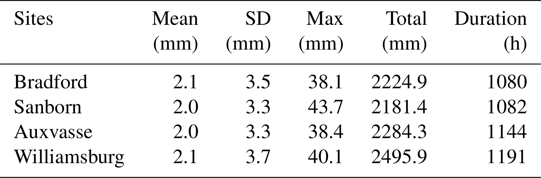
Table 1 summarizes the characteristics of rainfalls observed at Bradford, Sanborn, Auxvasse, and Williamsburg between April 2016 and June 2018. It is clear that the hourly rain amounts are dominated by light rain, with similar means of 2.0–2.1 mm at the four sites, indicating uniformly distributed rainfalls within the experimental region. On the other hand, the standard deviations of Bradford and Williamsburg are 3.5 and 3.7 mm, respectively, a little larger than that of 3.3 mm at Sanborn and Auxvasse. Moreover, Sanborn gives the highest hourly rain amount, the lowest total rain amount, and the second lowest duration out of the four sites, due to the effects of the urban heat island (Hubbart et al., 2014). The second highest maximum hourly rain amount is recorded at Williamsburg; however, the total rain amount and duration are also the highest among the four sites, implying that convective rain is the most frequent at Williamsburg. In contrast, stratiform rain is more common at Bradford, since the gauge records the lowest maximum hourly rain amount and duration, as well as the second total hourly rain amount. In addition, it can be seen that Auxvasse also provides useful data for the comparisons between gauges and between the radar and gauge, though the statistics are all ranked in the middle of the four sites. Overall, the rain gauge data at Bradford, Sanborn, Auxvasse, and Williamsburg are representative and sufficiently large, leading to a valid dataset for testing the K_dp and K_dp-based rain amounts.

4 K_dp retrieval

As discussed in Sect. 2, the joint probability density function (PDF) based on a Gaussian mixture can be used to derive the regression model for K_dp estimation. The Gaussian mixture method (GMM) not only estimates the expected values of K_dp by differentiating the conditional expectation of Φ_dp, but also gives an estimation of K_dp variance by regarding the errors in the calculation of the first derivative of Φ_dp. In this section, we describe GMM for the K_dp estimation using MZZU radar data. Figure 1 illustrates the flowchart of GMM (Fig. 1b), comparing to that of the linear regression model (LR; Fig. 1a).

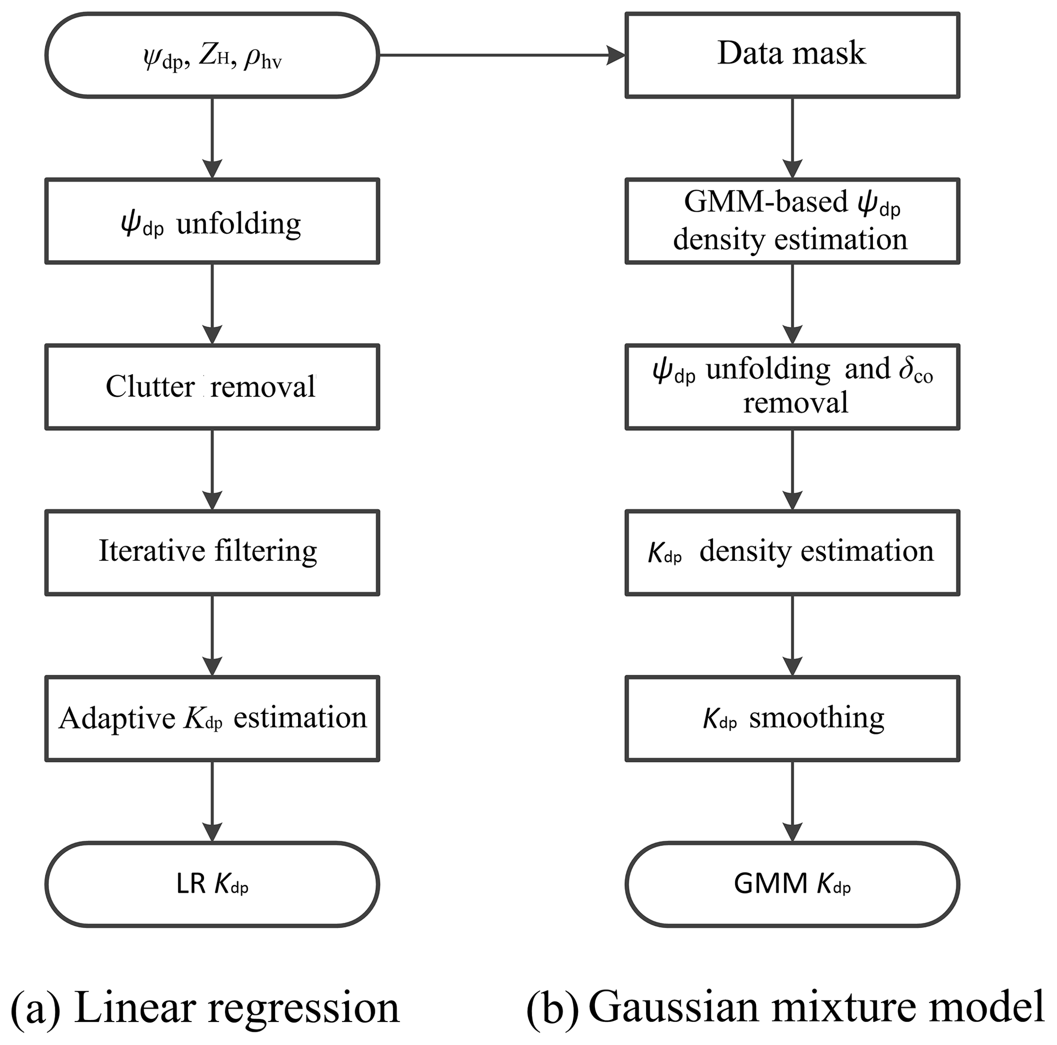
Figure 1 Flowcharts of K_dp estimation algorithms used in the MZZU radar: (a) linear regression model and (b) Gaussian mixture method.

From the chart of LR in Fig. 1a, we can see that after the radar measurements are collected, the Ψ_dp is unfolded and then the clutter is removed. After these corrections, an iterative filtering method is applied to the Ψ_dp profile. An adaptive method is finally used to estimate the K_dp profile according to the values of Z_H. The Gaussian mixture model, on the other hand, processes Ψ_dp differently. First of all, the clutter is masked out according to the thresholds of Z_H and the variation of Ψ_dp. Secondly, the range r and Ψ_dp are fitted into a Gaussian mixture to yield the joint PDF, while the Ψ_dp mean and the Ψ_dp variance are obtained by taking the first raw and second central moments of the conditional PDF of Ψ_dp given r. Thirdly, some specific clusters in the Gaussian mixture PDF are adjusted to solve the problems of ambiguous Ψ_dp and backscattering differential phase shift δ_co in order to derive the PDF of Φ_dp. Fourthly, a raw K_dp profile is calculated from the first derivative of the expected values of Φ_dp, and the associated variances are obtained via a Taylor series expansion. Finally, the raw K_dp profile is smoothed, and, consequently, the variances are reduced. In addition, new Φ_dp with lower variances can be reconstructed from the K_dp estimates.

4.1 Data masking

The presence of clutter in the Ψ_dp measurements may severely affect the K_dp estimation, producing significantly large variations on the estimates. It is well known that the effect of clutter can be reduced by applying a spectrum filter to the time-series data (e.g.,  May and Strauch, 1998; Hubbert et al., 2009). However, some residual clutter echoes are still shown on the radar measurements including Ψ_dp (Wen et al., 2017). Therefore, the clutter needs to be well handled in GMM, prior to the deviation of the regression model based on the joint PDF.

In LR, the clutter is often eliminated by some criteria based on Ψ_dp or ρ_hv. For instance, we use the thresholds of the local standard deviation of Ψ_dp less than 10^∘ to classify valid points. Further, 10 consecutive range gates of valid points signify the beginning of a rain cell, and 5 consecutive gates of invalid points finish the associated rain cell. Overall, the thresholds give a fairly good performance on the MZZU radar; however, the clutter may be incorrectly identified in the regions of high reflectivity or for the echoes mixed by weather and clutter, which are often associated with large Ψ_dp variation.

Figure 2 Flowchart of data masking.

In contrast, GMM adopts sophisticated procedures, as depicted in Fig. 2. It is clear that there are five stages in the data masking, beginning with the input of raw Ψ_dp and ending with masked data. At the first stage, the raw data are fitted to a Gaussian mixture initialized by the k-means clustering, while the covariance is set to be diagonal for simplicity. The clusters with no more than five points are promptly masked out, before they pass to the second stage. Stages two, three, and four of the process all involve the clusters. At the second stage, the clusters are validated according to two sets of thresholds with respect to mean reflectivity. For the MZZU radar, the ratio of the standard deviations, σ(Ψ_dp)∕σ(r), less than 14.2^∘ km⁻¹ and σ(Ψ_dp) less than 4.1^∘ (threshold 2) are used for Z_H less than 41 dBZ. To reduce the misclassification in the hail regions, the thresholds are increased for higher Z_H, resulting in $\mathit{\sigma }\left({\mathrm{\Psi }}_{\mathrm{dp}}\right)/\mathit{\sigma }\left(r\right)<\mathrm{47.9}$^∘ km⁻¹ and σ(Ψ_dp)<6.3^∘ (threshold 1). Next, the entire Ψ_dp profile is divided into multiple rain cell segments by considering the gaps between two consecutive clusters. Similar to the first stage, the segments containing no more than five points are excluded from the output of masked data. Following this, the dominant one is determined for each segment by comparing the weight accumulations of weather and clutter clusters. For a clutter segment with mean height below 200 m, the clusters within the segment are reevaluated by thresholds of $\mathit{\sigma }\left({\mathrm{\Psi }}_{\mathrm{dp}}\right)/\mathit{\sigma }\left(r\right)<\mathrm{2.0}$^∘ km⁻¹ and σ(Ψ_dp)<0.8^∘; on the other hand, the clusters in a weather segment are reexamined using $\mathit{\sigma }\left({\mathrm{\Psi }}_{\mathrm{dp}}\right)/\mathit{\sigma }\left(r\right)<\mathrm{34.7}$^∘ km⁻¹ and σ(Ψ_dp)<6.1^∘. This step can efficiently identify the clutter-contaminated weather echoes, which are often associated with large variances. At the last stage, some isolated points along the azimuth are obscured in the final results.

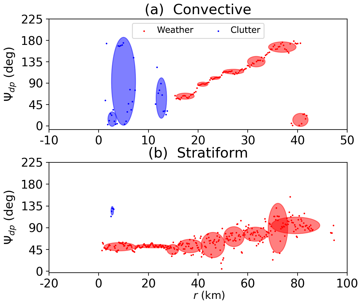
Figure 3 Examples of data masking: (a) a convective case (azimuth 252^∘) and (b) a stratiform case (azimuth 1^∘). The blue points and ellipses represent the clutter data and clusters, respectively, while the red color corresponds to the weather echoes. The x axis is the radar range in kilometers.

Figure 3 illustrates two examples for data masking, including a convective case (Fig. 3a) and a stratiform case (Fig. 3b). The data points in the two cases show steadily increasing trends related to anisotropic media along the wave propagation path. However, between 1.3 and 15 km at an azimuth of 252^∘ in the convective case (Fig. 3a), the data present significant fluctuations with the minimum value at about 0^∘ but the maximum value at 180^∘. Since the dynamic range of Ψ_dp is from 0 to 180^∘ for the MZZU radar, the measurements near the ground are likely to be the clutter returns, verifying the results of data masking. After 15 km, the Ψ_dp points start from about 50^∘ and go all the way up to 180^∘. Notwithstanding this trend, the points sharply decrease to about 10^∘ at about 40 km, indicating the occurrence of phase folding. The data masking can effectively detect the phase folding and provide valid masked data for deriving the joint PDF. On the other hand, the weather echoes are more frequently observed at 1^∘ in azimuth in the stratiform case (Fig. 3b). By taking a closer look at the Ψ_dp data, we can discern that the points largely fluctuate between 40 and 80 km due to low signal-to-noise ratio. In LR, these points may be incorrectly discarded based on σ(Ψ_dp) thresholds, leading to some missing data in the stratiform regions. In contrast, the data masking accurately identifies weather echoes characterized by a number of vertically oriented density ellipses. The continuous and uniformly distributed regimes are consistent with the physical interpretation of stratiform precipitation. In addition, the data masking is also sensitive to sudden jumps at the beginning of the Ψ_dp data, which may be caused by δ_co.

4.2 Ψ_dp density estimation

In the previous section, it is shown that the Ψ_dp profile varies along the range r. It rises quickly for horizontally oriented anisotropic scatterers, and, conversely, it falls steadily for vertically oriented particles (Marzano et al., 2010). The nonuniform beam filling is also an important source of errors for the Ψ_dp measurements (Gosset, 2004; Ryzhkov, 2007).

To estimate the relationship between r and Ψ_dp, we consider r as an independent variable, denoted as x, and Ψ_dp as a dependent variable, denoted as y. If the minimization of the mean square error is required, the regression function is obtained by taking the average value of y at fixed x, equivalent to estimating the expected values of y conditioned on x; i.e.,

$$\begin{array}{}\text{(10)}& \stackrel{\mathrm{‾}}{y}\left(x\right)=E\left(y\right|x)=\int yp(y|x,\mathit{\beta })\mathrm{d}x,\end{array}$$

where β is a set of unknown variables – for example, $\mathit{\beta }=(m,w,\mathit{\mu },\mathbf{\Sigma })$ for the mixture model. Since the Gaussian mixture can be used to model any shapes of probability density with a rapid speed, the (x, y) points are then assumed to follow a joint PDF of Gaussian mixture, as defined in Eq. (4). Moreover, the properties of the multivariate Gaussian distribution in each cluster determine the Gaussianity of the marginal distribution of either variable and the conditional distribution of one variable given the other (Bishop, 2006). Therefore, the conditional PDF of y given x is expressed as

$$\begin{array}{}\text{(11)}& {\displaystyle }p\left(y\right|x,\mathit{\beta })& {\displaystyle }=\sum _{i=\mathrm{1}}^m{w}_i^{y|x}\mathcal{N}\left(y;{\mathit{\mu }}_i^{y|x},{\mathrm{\Sigma }}_i^{y|x}\right),\text{with}\text{(12)}& {\displaystyle }{\mathit{\mu }}_i^{y|x}& {\displaystyle }={\mathit{\mu }}_i^y+{\mathrm{\Sigma }}_i^{yx}\left({\mathrm{\Sigma }}_i^{xx}{)}^{-\mathrm{1}}\right(x-{\mathit{\mu }}_i^x),\text{(13)}& {\displaystyle }{\mathrm{\Sigma }}_i^{y|x}& {\displaystyle }={\mathrm{\Sigma }}_i^{yy}-{\mathrm{\Sigma }}_i^{yx}({\mathrm{\Sigma }}_i^{xx}{)}^{-\mathrm{1}}{\mathrm{\Sigma }}_i^{xy},\text{(14)}& {\displaystyle }{w}_i^{y|x}& {\displaystyle }={\displaystyle \frac{f_i\left(x\right)}{f\left(x\right)}}={\displaystyle \frac{w_i\mathcal{N}(x;{\mathit{\mu }}_i^x,{\mathrm{\Sigma }}_i^{xx})}{{\sum }_{j=\mathrm{1}}^m{w}_j\mathcal{N}(x;{\mathit{\mu }}_j^x,{\mathrm{\Sigma }}_j^{xx})}},\end{array}$$

where w_i, ${\mathit{\mu }}_i=({\mathit{\mu }}_i^x,{\mathit{\mu }}_i^y{)}^T$ and ${\mathbf{\Sigma }}_i=\left(\begin{array}{cc}{\mathrm{\Sigma }}_i^{xx}& {\mathrm{\Sigma }}_i^{xy}\\ {\mathrm{\Sigma }}_i^{yx}& {\mathrm{\Sigma }}_i^{yy}\end{array}\right)$ are obtained by the EM algorithm. In Eq. (14), f(x) is the marginal PDF of x with the parameters identical to the mixture, and f_i(x) is the weighted marginal PDF of each cluster; i.e., $f\left(x\right)={\sum }_{i=\mathrm{1}}^m{f}_i\left(x\right)$. By substituting Eq. (11) into Eq. (10) and noting the linearity of the mathematical expectation, the expected value of y conditioned on x is then obtained as

$$\begin{array}{}\text{(15)}& {\displaystyle }E\left(y\right|x)& {\displaystyle }=\sum _{i=\mathrm{1}}^m{\displaystyle \frac{f_i\left(x\right)}{f\left(x\right)}}(a_{i}x+b_i),\text{with}\text{(16)}& {\displaystyle }{a}_i& {\displaystyle }={\mathrm{\Sigma }}_i^{yx}({\mathrm{\Sigma }}_i^{xx}{)}^{-\mathrm{1}},\text{(17)}& {\displaystyle }{b}_i& {\displaystyle }={\mathit{\mu }}_i^y-{\mathrm{\Sigma }}_i^{yx}({\mathrm{\Sigma }}_i^{xx}{)}^{-\mathrm{1}}{\mathit{\mu }}_i^x,\end{array}$$

and the conditional variance is given as (see Appendix B)

$$\begin{array}{}\text{(18)}& \begin{array}{rl}{\mathit{\sigma }}^{\mathrm{2}}\left(y\right|x)& =\sum _{i=\mathrm{1}}^m{w}_i^{y|x}\left[{\mathrm{\Sigma }}_i^{y|x}+{\left({\mathit{\mu }}_i^{y|x}\right)}^{\mathrm{2}}\right]\\ & -{\left(\sum _{i=\mathrm{1}}^m{w}_i^{y|x}{\mathit{\mu }}_i^{y|x}\right)}^{\mathrm{2}}.\end{array}\end{array}$$

Equations (15) and (18) play an important role in the joint PDF-based regression analysis, called the regression and skedastic functions (Spanos, 1999). In Eq. (15), it can be seen that the regression function in GMM consists of multiple linear kernels, which is similar to LR. However, the weighting function $w_i^{y|x}$ is not determined by the local structure but the marginal PDF of global data x. The Gaussian mixture method is flexible to capture the data information, while it still retains a finite set of parameters. Moreover, Eq. (18) readily estimates the point-wise variances σ²(y|x) that characterize the random errors in the measurements. In contrast, Eq. (3) for the LR presents the relationship between the errors σ(Ψ_dp) and σ(K_dp) under the ideal conditions, which does not consider the random errors in Ψ_dp. It indicates that the GMM has a better error characterization based on the measurements when compared to the LR.

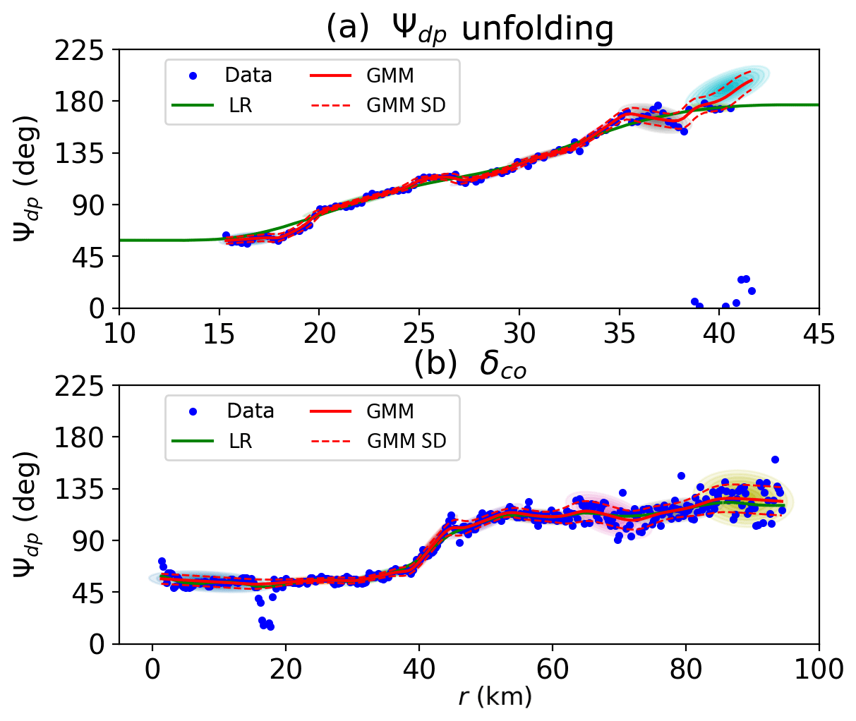
Figure 4 Examples of Ψ_dp density estimation: (a) a Ψ_dp unfolding case and (b) a δ_co case. The blue points are the Ψ_dp data, the green curve represents the Ψ_dp profile obtained by the linear regression model (LR), and the red curve indicates the Ψ_dp profile produced by the Gaussian mixture method (GMM). The dashed lines are the standard deviations, while the colored ellipses show the components of the Gaussian mixture. The x axis is the radar range in kilometers.

Figure 4 compares the Ψ_dp profiles given by Eqs. (15) and (18) with that obtained by LR. Figure 4a gives the same example as Fig. 3a, but the EM algorithm is configured differently. In the Ψ_dp density estimation, the mixture with full covariance yields density ellipses of random shapes. Furthermore, the algorithm repeats the fitting procedures three times to avoid the local maxima of the log-likelihood. Meanwhile, the choice of the cluster number relies on the Bayesian information criterion calculated for each m, starting at 10 clusters. It can be seen that the mixture composed by density ellipses characterizes the data points well, since the root-mean-square error is small relative to the expected values. Between 15 and 35 km, the narrow ellipses result in Ψ_dp with a rising trend consistent with LR. On the other hand, the mixture has very small variances, giving a high confidence for the fitted parameters. From 35 km, the ellipses become wider, and the associated variances increase due to the low signal-to-noise ratio at the edge of radar echoes. What is notable, however, is that the Ψ_dp profile dramatically increases to a large value, whereas LR remains a relatively steady trend. It indicates the importance of the Ψ_dp unfolding for the Ψ_dp density estimation.

Figure 4b presents another example of the density estimation. It is clear that the Ψ_dp profiles produced by GMM and LR both rise considerably along the range, and the trends for the two methods are very similar with a strong correlation of 0.998. The profile starts at about 50^∘ and remains relatively stable before rising dramatically between 35 and 55 km. By 65 km, Ψ_dp has more than doubled, and then there is a steady increase for Ψ_dp reaching about 130^∘ at the end of the profile, which is around 70^∘ up on the ranges of 0 and 35 km, and 10^∘ more than recorded at the ranges of 55 and 65 km. If we examine Ψ_dp measured at X-band frequency, we can see that some points fall out of the dashed lines corresponding to 1 standard error (i.e., 95 % interval). Most notably, the Ψ_dp profile shows a sudden slump between 18 and 20 km, while the Z_DR corresponds to a local peak (not shown). It may indicate the occurrence of δ_co. In conclusion, the expected value and the variance of Ψ_dp can be obtained from the joint PDF, but the mixture needs to be tuned in terms of Ψ_dp unfolding and δ_co elimination in order to obtain the PDF of Φ_dp.

4.3 Ψ_dp unfolding and δ_co elimination

According to the continuity and consistency of the phase data, we can discern that some issues exist in the density estimation, such as ambiguous Ψ_dp and δ_co. Since Ψ_dp is a range accumulative measurement of the propagation phase, depending on the initial Ψ_dp(0), the measurements may exceed the dynamic range of 0–180^∘ when the wave propagates through a rain medium. This situation is even more significant at X-band frequency than at S-band due to the inverse relation of the wavelength and the rate of phase shift. Nevertheless, it can be noted that Ψ_dp gives a nonnegative trend along the range for rain, and therefore the ambiguous Ψ_dp may be corrected accordingly (Wang and Chandrasekar, 2009).

In LR, Ψ_dp is first averaged over a small window for weather data, and a linear fit is then performed to obtain the increment for the range gate next to the window. In the following stage, a reference is predicted by summing up the average and the increment and compared to the observed value at the same gate. If the difference between the predicted and observed values is larger than 90^∘, the observed Ψ_dp is then increased by 180^∘. Finally, the correction process is iteratively operated until the last gate.

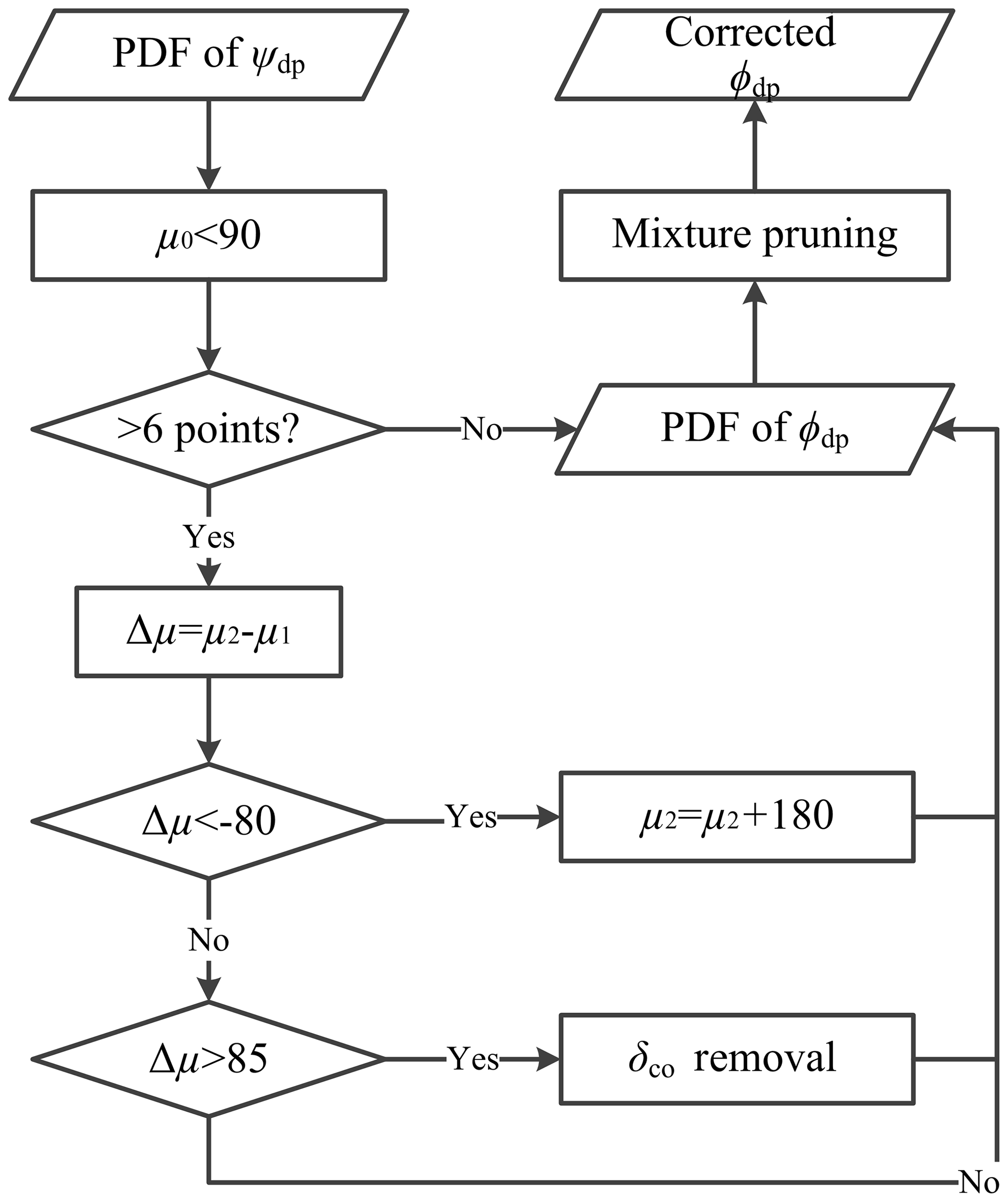
Figure 5 Flowchart of the Ψ_dp unfolding and the δ_co elimination. The μ₀ is the mean of the first density ellipse. The μ₁ and μ₂ are the means of the two consecutive density ellipses along the range. The μ₁ is the mean of the former one, and the μ₂ is the mean of the latter one.

On the other hand, the Ψ_dp unfolding is more straightforward in GMM. Figure 5 shows the flowchart of the Ψ_dp unfolding and the δ_co elimination. After obtaining the PDF of Ψ_dp, the initial step of the Ψ_dp unfolding selects the density ellipses with at least six data points. Next, the second step calculates the difference of the means μ_i between the two consecutive density ellipses along the range. At this point, the PDF of Ψ_dp is ready to be corrected for ambiguous Ψ_dp. In the final step, the mean of the latter density ellipse is added up 180^∘, if the former mean is larger than the latter one by 80^∘.

As illustrated in Fig. 4a, the profile Ψ_dp reaches 180^∘ at about 38 km and then becomes ambiguous between 38 and 42 km. In LR, the Ψ_dp values at these locations are interpolated according to the trend of the previous few gates, and the maximum value is 180^∘. In contrast, the corrected density ellipses in GMM show an upward trend between 38 and 42 km, while the Ψ_dp profile reaches a maximum value of about 195^∘, indicating the effectiveness of the Ψ_dp unfolding in the region of heavy rain. In addition, when we apply the algorithm to a larger dataset, the rate of false alarm reaches a very small value at 0.66 %.

In addition to the ambiguous Ψ_dp, the estimation of the joint PDF may also be affected by nonzero δ_co, which is defined as the phase difference between the horizontal and vertical polarizations upon the backscattering of the particles in a radar resolution volume. This effect occurs more frequently at X-band frequency than S-band due to Mie scattering (Trömel et al., 2013). The δ_co is shown as a sudden phase change over a small number of gates in a monotonically increasing trend for rain. According to this manifestation, the magnitude and gate number of the Ψ_dp perturbation can be used to eliminate δ_co (Matrosov et al., 2002; Otto and Russchenberg, 2011).

The linear regression model often adopts an iterative filter technique, which generates a new Φ_dp profile from either the raw data or the filtered one based on a threshold (Hubbert and Bringi, 1995). If the filtering alters the data by 4^∘, the new profile selects the filtered data; otherwise the raw data remain. The new profile is then used as input in the next iteration until the convergence condition is satisfied.

As shown in Fig. 5, the δ_co elimination is embedded into the process of the Ψ_dp unfolding. For two consecutive density ellipses, the latter density ellipse is removed if its mean is larger than the former one by 85^∘. Prior to this step, the mean of the first density ellipse in the mixture should be below 90^∘ to reduce the δ_co effect at the first few gates. Since δ_co occurs over a small number of range gates, a mixture pruning is also employed to remove the density ellipses with weights less than 0.0501, equivalent to 2 % of the data.

It is clear from Fig. 4b that δ_co has occurred at multiple locations in the data. The Ψ_dp profile starts at a high value and drops somewhat over the first two gates. Notably, there is a narrow gap between 18 and 20 km, while the corresponding Z_DR presents a local peak. It signifies that nonzero δ_co occurs in this region. In GMM, these data are characterized by a density ellipse with a slightly decreasing trend, and the resulting expected values are consistent with the filtered data in LR. Between 70 and 90 km, a few isolated points beyond the density ellipses are associated with δ_co. Both of the methods can produce Φ_dp following the main trend of the data, which suggests that the process is effective for the δ_co elimination.

4.4 K_dp density estimation

As discussed in Sect. 2.1, K_dp is the first derivative of Φ_dp with respect to the range r. According to the mean value and dominated convergence theorems, the derivative of the expected value of Φ_dp conditioned on r is equal to the expected value of the derivative of Φ_dp with respect to r, i.e., K_dp (see Appendix C). Following the notation in Sect. 4.2, we denote K_dp as y^′. Therefore, the expected value of K_dp is obtained by taking the derivative of Eq. (15), yielding

$$\begin{array}{}\text{(19)}& \begin{array}{rl}& E\left(\left.y^{\prime }\right|x\right)={\displaystyle \frac{\mathrm{1}}{f^{\mathrm{2}}\left(x\right)}}\left\{\sum _{i=\mathrm{1}}^m\sum _{j=\mathrm{1}}^m{f}_i\left(x\right)f_j\left(x\right)\right.\\ & \left.\left[\left({\displaystyle \frac{x-{\mathit{\mu }}_j^x}{{\mathrm{\Sigma }}_j^{xx}}}-{\displaystyle \frac{x-{\mathit{\mu }}_i^x}{{\mathrm{\Sigma }}_i^{xx}}}\right)(a_{i}x+b_i)+a_i\right]\right\}.\end{array}\end{array}$$

The variance of y^′ conditioned on x can be approximated by the first-order Taylor series expansion (see Appendix D); i.e.,

$$\begin{array}{}\text{(20)}& {\mathit{\sigma }}^{\mathrm{2}}\left(y^{\prime }|x\right)={\left[E^{\prime \prime }\left(y\right|x)\right]}^{\mathrm{2}}{\mathit{\sigma }}^{\mathrm{2}}\left(y\right|x),\end{array}$$

where σ²(y|x) is given in Eq. (18). By taking the derivative of Eq. (19), $E^{\prime \prime }\left(y\right|x)$ is expressed as

$$\begin{array}{}\text{(21)}& E^{\prime \prime }\left(y\right|x)=\mathrm{2}\left[\sum _{i=\mathrm{1}}^m{a}_i{\left(w_i^{y|x}\right)}^{\prime }\right]+\sum _{i=\mathrm{1}}^m(a_{i}x+b_i){\left(w_i^{y|x}\right)}^{\prime \prime }.\end{array}$$

From Eq. (C8) in Appendix C, it is clear that

$$\begin{array}{}\text{(22)}& \begin{array}{rl}& {\left(w_i^{y|x}\right)}^{\prime }={\displaystyle \frac{g_i\left(x\right)}{f^{\mathrm{2}}\left(x\right)}}={\displaystyle \frac{\mathrm{1}}{f^{\mathrm{2}}\left(x\right)}}\sum _{j=\mathrm{1}}^m{f}_j\left(x\right)\\ & f_i\left(x\right)\left({\displaystyle \frac{x-{\mathit{\mu }}_j^x}{{\mathrm{\Sigma }}_j^{xx}}}-{\displaystyle \frac{x-{\mathit{\mu }}_i^x}{{\mathrm{\Sigma }}_i^{xx}}}\right),\end{array}\end{array}$$

where g_i(x) is the summation term. Subsequently, the second derivative of $w_i^{y|x}$ is given as

$$\begin{array}{}\text{(23)}& {\displaystyle }{\left(w_i^{y|x}\right)}^{\prime \prime }={\displaystyle \frac{g_i^{\prime }\left(x\right)f\left(x\right)-\mathrm{2}{f}^{\prime }\left(x\right)g_i\left(x\right)}{f^{\mathrm{3}}\left(x\right)}},\text{where}\text{(24)}& {\displaystyle }{f}^{\prime }\left(x\right)=-\sum _{j=\mathrm{1}}^m\left({\displaystyle \frac{x-{\mathit{\mu }}_j^x}{{\mathrm{\Sigma }}_j^{xx}}}\right)f_j\left(x\right),\text{(25)}& {\displaystyle }\begin{array}{rl}{g}_i^{\prime }\left(x\right)& =\sum _{j=\mathrm{1}}^m{f}_j\left(x\right)f_i\left(x\right)\left[{\left({\displaystyle \frac{x-{\mathit{\mu }}_i^x}{{\mathrm{\Sigma }}_i^{xx}}}\right)}^{\mathrm{2}}-{\left({\displaystyle \frac{x-{\mathit{\mu }}_j^x}{{\mathrm{\Sigma }}_j^{xx}}}\right)}^{\mathrm{2}}\right.\\ & \left.+{\displaystyle \frac{\mathrm{1}}{{\mathrm{\Sigma }}_j^{xx}}}-{\displaystyle \frac{\mathrm{1}}{{\mathrm{\Sigma }}_i^{xx}}}\right].\end{array}\end{array}$$

Equations (19) and (20) are the regression and skedastic functions for the K_dp estimation. In Eq. (19), it is clear that the expected value of K_dp can be divided into two components, including Eqs. (C7) and (C11). On the one hand, Eq. (C7) is related to the changing rate a_i weighted by the marginal distribution of each cluster in the mixture, equivalent to a linearly weighted combination of small portions of data. If a data point is dominated by a specific cluster, i.e., the weight of a cluster is significantly larger than the others, K_dp is determined by the coefficients of the cross-correlation and auto-correlation of r, and independent of the means and auto-correlation of Φ_dp, yielding a constant value within the dominated cluster. On the other hand, Eq. (C11) shows that the weighting function also contributes to the K_dp estimates by considering the Gaussian derivative of the Φ_dp estimates in two or three adjacent clusters along the range. The sign of K_dp is then determined by the marginal means and variances of the clusters, weighted by the difference of their contributions to Φ_dp.

In Eq. (20), it can be seen that σ²(K_dp) is proportional to σ²(Φ_dp), which is similar to Eq. (3). When the LR is applied to the MZZU radar, we often assume that σ(Φ_dp) is equal to 2.61^∘ with 32 pulses, 1 m s⁻¹ for Doppler spectrum and 0.98 for ρ_hv under the ideal conditions. However, in the GMM, σ²(Φ_dp) varies along the range due to the random errors of the Φ_dp estimates, indicating the GMM can provide a better model for the error characteristics in the Φ_dp measurements. In addition, the statistical errors with respect to signal processing may be included in Eq. (20) as an additive term, independent of Φ_dp. Moreover, σ²(K_dp) in GMM is closely related to the first derivative of K_dp in Eq. (20). As the changing rate of K_dp increases, the random errors associated with the K_dp estimates rise dramatically.

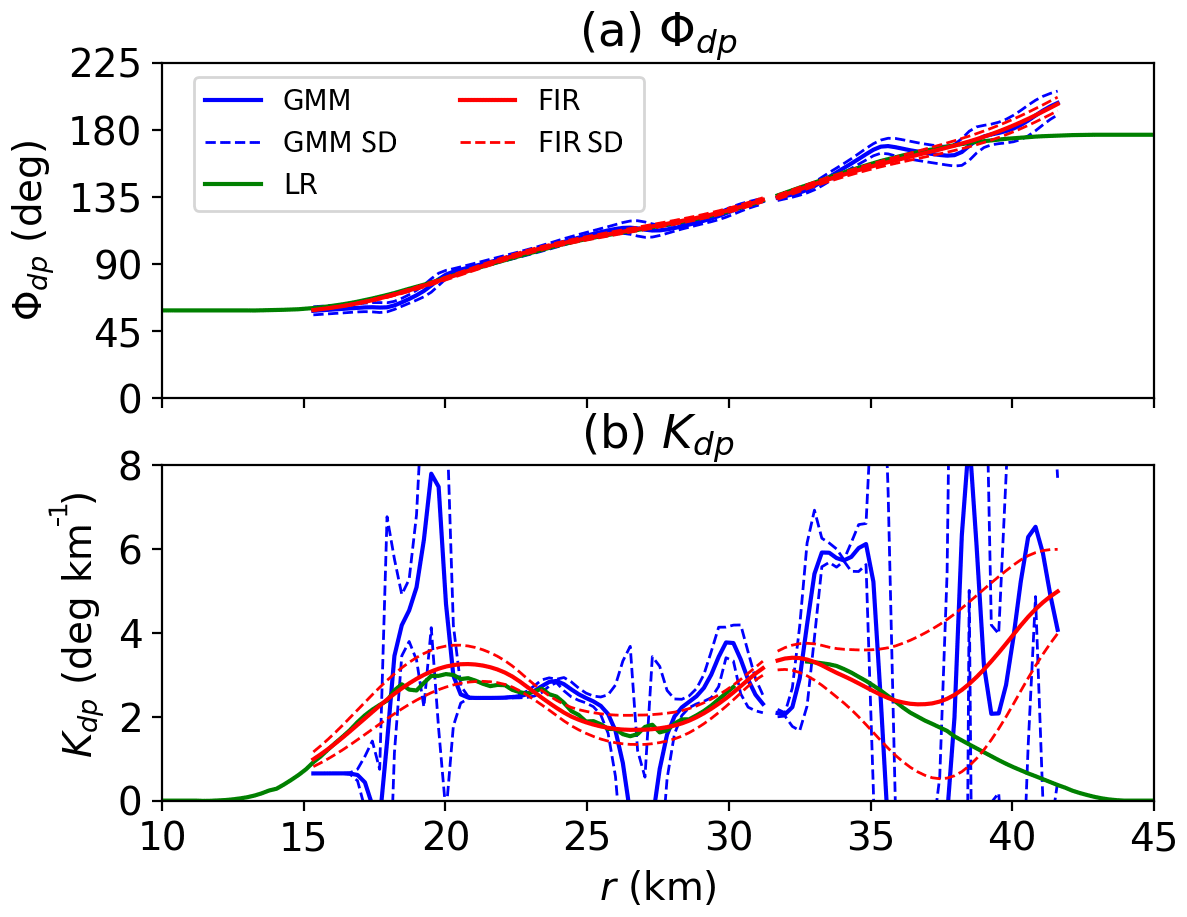
Figure 6 Examples of K_dp estimation: (a) Φ_dp and (b) K_dp. The blue curves are the Φ_dp and K_dp estimates obtained by the Gaussian mixture method (GMM), the green curves represent the estimates derived from the linear regression model (LR), and the red curves indicate the reconstructed Φ_dp and smoothed K_dp profiles (FIR). The dashed lines are the standard deviations.

Figure 6b illustrates K_dp and its variance estimated from Φ_dp in Fig. 6a, which is the same case as given in Figs. 3a and 4a. It is apparent that the K_dp estimates present a large fluctuation, while the associated variances are significant. In GMM, K_dp starts from about 0.5 ^∘ km⁻¹ and then fluctuates between 17 and 20 km and between 24 and 42 km. In the profile, there are six local peaks with the maximum at about 8.5 ^∘ km⁻¹. Meanwhile, the K_dp variances vary as the K_dp estimates change. Between 15 and 17 km and between 20 and 24 km, the K_dp estimates remain constant, leading to small K_dp variances in these regions. When short excursions are present, such as that between 18 and 20 km, K_dp variances increase significantly due to the contribution of the first derivative of K_dp in Eq. (20). Furthermore, the large Φ_dp variances between 35 and 42 km also result in an increase in the K_dp variances. In contrast, LR gives less fluctuation in K_dp estimates with two peaks at about 20 and 34 km. The comparison of K_dp obtained by the two methods may suggest that a smoothing procedure is required to reduce the significant variance in GMM.

4.5 K_dp smoothing

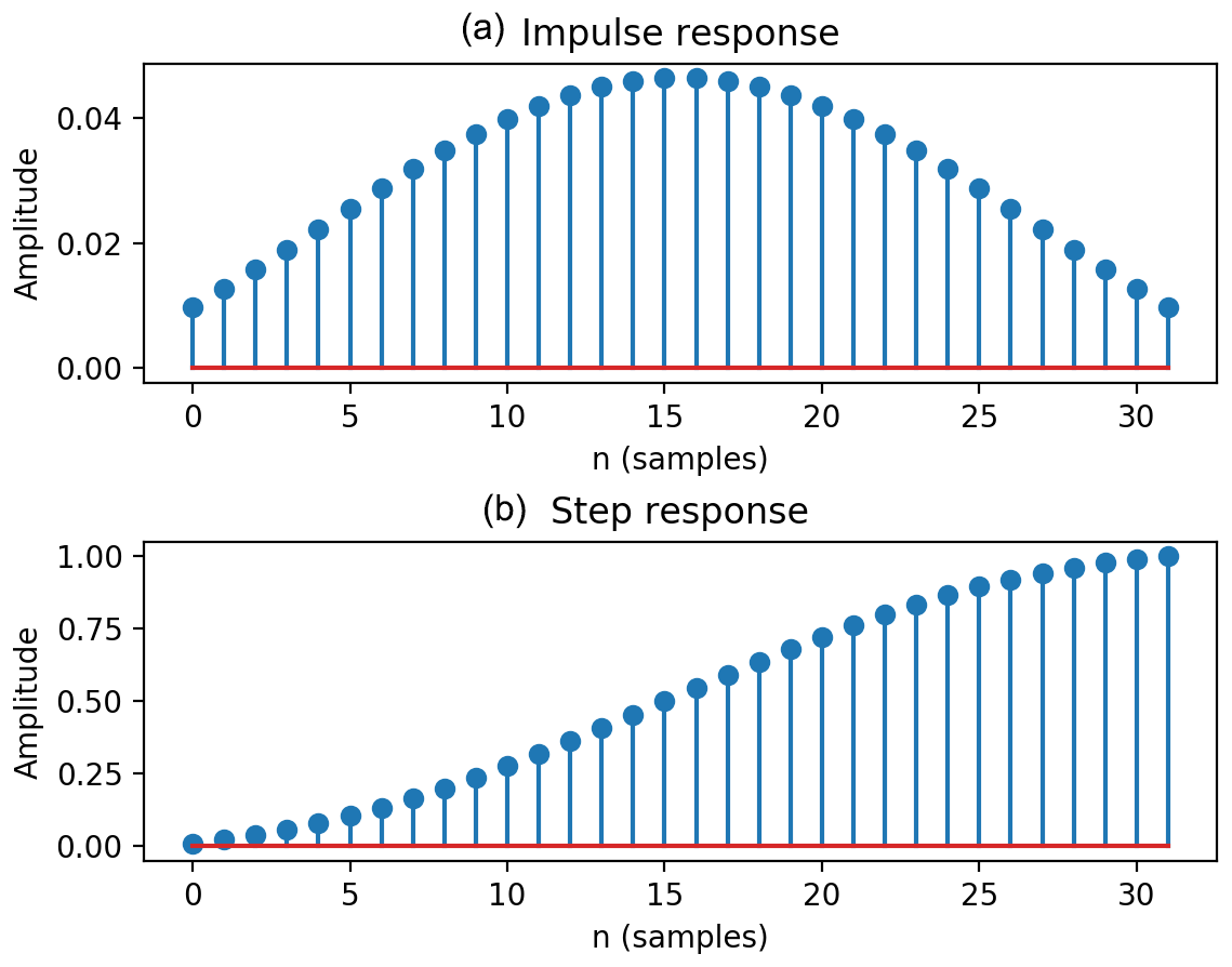
As discussed previously, the K_dp variance is small for high K_dp but relatively large for low K_dp. Therefore, an adaptive estimation is adopted in LR. For radar reflectivity (Z_H) less than 20 dBZ, the gate number n in Eq. (2) is set as 15, while n is 8 for $\mathrm{20}\le Z_H<\mathrm{35}$ dBZ and 2 for Z_H≥35 dBZ. On the other hand, GMM also applies an adaptive technique based on the finite impulse filter (FIR) to the expected values of K_dp in order to reduce the associated variances. Figure 7 shows the time responses of the FIR with the cutoff frequency of 0.053 and the Gaussian window of 28, which yield the best performance for the MZZU radar. The impulse response (Fig. 7a) is peaked at the center and gradually decreases towards the two ends. Furthermore, the step response (Fig. 7b) gives the accumulation of the impulse response, indicating that the magnitudes around the center change faster than those at the two ends. If a longer window is required, the order of the FIR is increased accordingly. In this study, we gradually increase the order number to calculate the difference between the K_dp profiles obtained by the FIR filters with two adjacent order numbers. The optimal order of the FIR filter is then set when the relative square error of the two K_dp values is below 0.001. For profiles with sufficiently large data points, the order number is between 29 and 33 for the MZZU radar.

Figure 7 Responses of finite impulse filter: (a) impulse response and (b) step response.

To obtain the reduced variance, we consider the filter as a number of weighting functions, denoted as h_i(x), and subsequently the smoothed data become

$$\begin{array}{}\text{(26)}& y=\sum _{i=\mathrm{1}}^n{h}_i*x_i,\end{array}$$

where y is a smoothed data point, x_i is the original data within the smoothing window, and n is the window length. By taking the variance on both sides of Eq. (26), we have

$$\begin{array}{}\text{(27)}& {\mathit{\sigma }}^{\mathrm{2}}\left(y\right)=\sum _{i=\mathrm{1}}^n{h}_i^{\mathrm{2}}{\mathit{\sigma }}^{\mathrm{2}}\left(x_i\right).\end{array}$$

Therefore, the variance of the smoothed data is the weighted sum of the variances of the original data within the smoothing window. Since the FIR coefficients are much less than unity, σ²(y) is smaller than σ²(x) at the same gate. Furthermore, the K_dp estimates with the reduced variances can be used to reconstruct Φ_dp to obtain smaller Φ_dp variances. For a fixed gate spacing Δr, the reconstructed Φ_dp for the jth range gate is

$$\begin{array}{}\text{(28)}& {\displaystyle }{\mathrm{\Phi }}_{\mathrm{dp}}^j& {\displaystyle }=\sum _{i=\mathrm{1}}^j{K}_{\mathrm{dp}}^i\mathrm{\Delta }r\text{and}\text{(29)}& {\displaystyle }{\mathit{\sigma }}^{\mathrm{2}}\left({\mathrm{\Phi }}_{\mathrm{dp}}^j\right)& {\displaystyle }=\sum _{i=\mathrm{1}}^j{\mathit{\sigma }}^{\mathrm{2}}\left(K_{\mathrm{dp}}^i\right)\mathrm{\Delta }{r}^{\mathrm{2}}.\end{array}$$

The red curves in Fig. 6a and b illustrate the reconstructed Φ_dp and the smoothed K_dp using FIR, respectively. The smoothed K_dp in Fig. 6b is more consistent with the LR results compared to the original K_dp produced by the GMM. In the first few kilometers, the smoothed K_dp gradually rises and then peaks at about 21 km. With no fluctuations, the smoothed K_dp falls gradually, followed by a growth before reaching a plateau at 33 km. After a slight decrease between 33 and 36 km, K_dp rises dramatically, which is very different from LR. Meanwhile, the variances are small at the beginning but get larger as K_dp is climbing. Between 20 and 33 km, the K_dp estimates do not change very much, leading to small variances in this region. But after 33 km, the variances begin to increase and retain large values until the end of the profile. Overall, the smoothed K_dp is stable, producing a profile considerably consistent with LR, and the variances are significantly reduced compared to the original data. In addition, the reconstructed Φ_dp (Fig. 6a) constantly increases with few local fluctuations, while the associated variances are smaller than the Φ_dp variances in GMM.

5 Evaluation

In this section, a case study is first presented to qualitatively analyze the storm structure and evolution based on K_dp. The radar–gauge dataset is then used to provide a quantitative evaluation for the K_dp estimation in terms of the root-mean-square error (RMSE), normalized bias (NB), and Pearson correlation coefficient (ρ_RG), which are defined as

$$\begin{array}{}\text{(30)}& {\displaystyle }\text{RMSE}& {\displaystyle }=\sqrt{{\displaystyle \frac{{\sum }_{i=\mathrm{1}}^N{\left(R_i-G_i\right)}^{\mathrm{2}}}{N}}},\text{(31)}& {\displaystyle }\text{NB}& {\displaystyle }={\displaystyle \frac{{\sum }_{i=\mathrm{1}}^N(R_i-G_i)}{{\sum }_{i=\mathrm{1}}^N{G}_i}},\text{(32)}& {\displaystyle }{\mathit{\rho }}_{\mathrm{RG}}& {\displaystyle }={\displaystyle \frac{{\sum }_{i=\mathrm{1}}^N(R_i-\stackrel{\mathrm{‾}}{R})(G_i-\stackrel{\mathrm{‾}}{G})}{\sqrt{{\sum }_{i=\mathrm{1}}^N(R_i-\stackrel{\mathrm{‾}}{R}{)}^{\mathrm{2}}}\sqrt{{\sum }_{i=\mathrm{1}}^N(G_i-\stackrel{\mathrm{‾}}{G}{)}^{\mathrm{2}}}}},\end{array}$$

where N is the sample size, R_i is the individual radar hourly rain amount, G_i is the gauge data, and $\stackrel{\mathrm{‾}}{R}$ and $\stackrel{\mathrm{‾}}{G}$ are the sample means for radar and gauge, respectively. The radar hourly rain amount is calculated based on the CASA radar rainfall algorithm. It is given as (Wang and Chandrasekar, 2010; Chen and Chandrasekar, 2015)

$$\begin{array}{}\text{(33)}& R\left(K_{\mathrm{dp}}\right)=\mathrm{18.15}{K}_{\mathrm{dp}}^{\mathrm{0.79}},\end{array}$$

where R is the instantaneous rain rate in millimeters per hour (mm h⁻¹). It is noted that the radar collects instantaneous measurements every 4–5 min, whereas RGs obtain the precipitation accumulations over 60 min. Therefore, it is necessary to average 12–15 consecutive radar scans to derive the hourly rain amounts.

5.1 Case study

On 24 March 2016, a severe storm developed in central Missouri and moved eastward across Columbia, MO, causing strong winds and heavy precipitation at the surface. When the storm became mature, the S-band radars at Kansas City and St. Louis observed the storm structure at high levels, since each radar was about 150 km away from the storm. Notably, the Kansas City radar showed positive and negative Doppler velocities in a small area (not shown), indicating the occurrence of a downburst. On the other hand, the MZZU radar illustrated a bow echo of Z_H close to the radar center (Fig. 8b). In addition to Z_H, the GMM-based K_dp (Fig. 8d, e and f) was also obtained to investigate the storm structure near the surface.

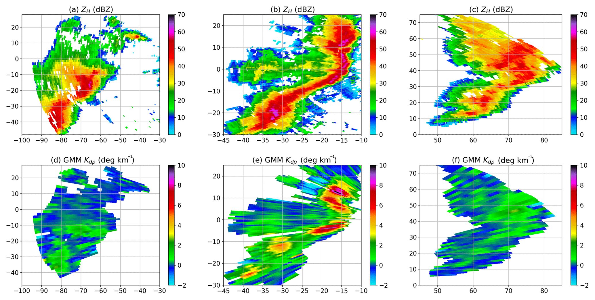
Figure 8 A case study for GMM: (a) raw Z_H at the development stage (03:04 UTC), (b) raw Z_H at the mature stage (03:39 UTC), and (c) raw Z_H at the dissipation stage (04:41 UTC). (d), (e), and (f) are the same as (a), (b), and (c), respectively, but for K_dp. The data were collected at a elevation of 0.85^∘ by the MZZU radar between 03:04 and 04:41 UTC on 24 March 2016.

Figure 8 illustrates that the convective storm evolves from a strong and large echo to a bow shape echo and then dissipates at far range. At 03:04 UTC (Fig. 8a), a cell with strong Z_H moves into the radar area, while K_dp is moderate with a maximum of about 3 ^∘ km⁻¹ (Fig. 8d). As the cell is transforming to a bow shape, the radar echo becomes intensive and forms a rain band with embedded convective cores (Fig. 8b). It is clear to see that K_dp reaches over 10 ^∘ km⁻¹ in these core regions (Fig. 8e), indicating very heavy precipitation at the surface. With the fast movement of the storm, the downburst is weaker, and the storm starts to dissipate (Fig. 8c). At 04:41 UTC, it can be seen that K_dp is gradually reduced at the far range, while its maximum is much lower than that at the mature stage.

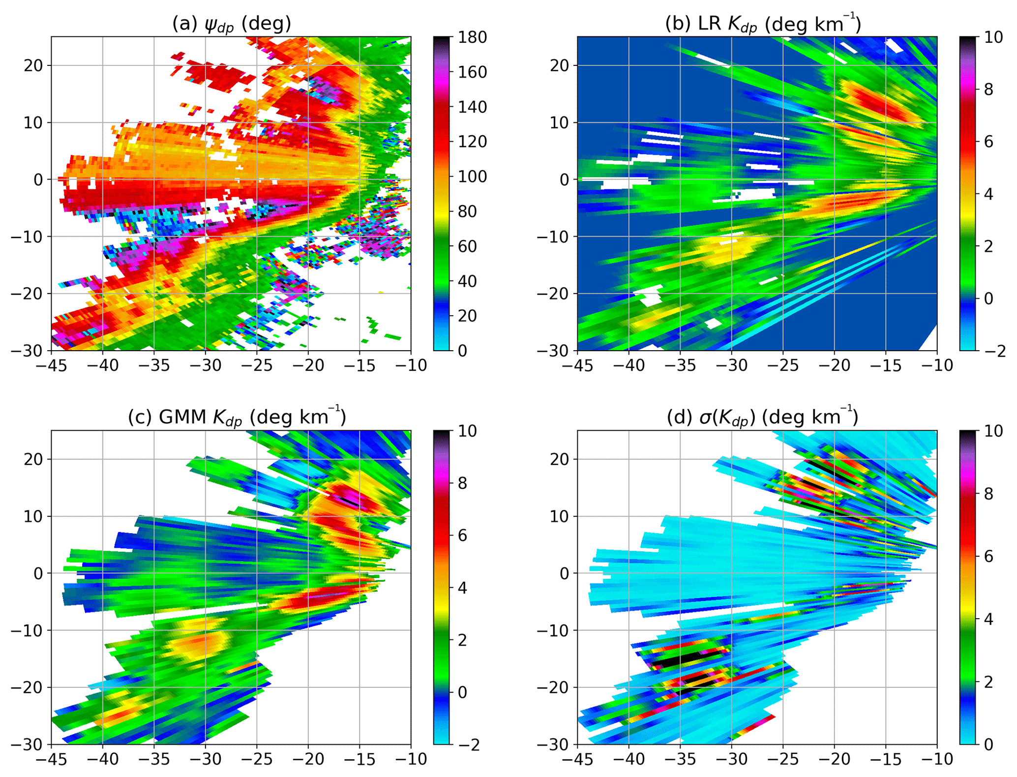
Figure 9 K_dp estimation for the mature stage: (a) raw Ψ_dp, (b) LR-based K_dp, (c) GMM-based K_dp, and (d) GMM-based σ(K_dp). The data were collected at 03:39 UTC on 24 March 2016.

In this storm, the bow echo is shown as a number of convective cores embedded in a rain band, while the downbursts occurred at the leading edge near the echo center. The bow echo can be considered as a mesoscale convection with a horizontal dimension of more than 60 km. To gain further insight, Fig. 9 shows raw Φ_dp and K_dp for the bow echo. In Fig. 9a, raw Φ_dp presents large gradients along the leading edge, rising from about 50^∘ to over 140^∘. Due to the sharp increase, Φ_dp exceeds the maximum dynamic range, leading to ambiguity in the areas of X of −20 to −18 km and Y of 12 to 18 km as well as X of −40 to −23 km and Y of −8 to −5 km. In addition, the echoes behind the convective cores occasionally vanish as a result of signal attenuation. Nevertheless, LR (Fig. 9b) produces continuous K_dp by Φ_dp unfolding and linear interpolation according to the trends of the profiles, but some missing data still exist within the storm, due to the low signal-to-noise ratio. In contrast, GMM (Fig. 9c) corrects these data with the expected values derived from the joint PDF and simultaneously obtains the statistical errors in the production of K_dp. It is evident that the GMM method can efficiently handle the missing data via the mixture model, which is another advantage over the LR model. Furthermore, the statistical errors are not very large in these areas, since the missing data are filled by the distribution of the entire data profile. Additionally, the GMM K_dp estimates are generally a few degrees per kilometer (^∘ km⁻¹) higher than the LR ones, particularly for the regions of high Z_H.

By taking a closer look at GMM K_dp, we can see that the bow echo is generally characterized by K_dp of above 2.5 ^∘ km⁻¹, while five pockets of high K_dp are identified. In the bow head, the first pocket presents very high K_dp associated with a rapid growth of Φ_dp. Behind this pocket, there is a region of negative K_dp, whereas LR generally yields positive values. It may be due to a reduction of the cross-correlation coefficient caused by the low signal-to-noise ratio, since the signals have been significantly attenuated after propagating through the pocket. In the middle of the second and third pockets in the bow center, LR and GMM both show lower K_dp compared to the two pockets, while K_dp is substantially consistent with the gradient of Φ_dp in the area. By considering the high Z_H in Fig. 8, these moderate K_dp values may indicate less anisotropic scatterers, such as small hail in the process of wet growth. Similarly, a hail signature with maximum Z_H of above 66 dBZ and small K_dp of 1–2 ^∘ km⁻¹ can also be identified in the middle of the fourth and fifth pockets in the bow tail. Along with the expected values of GMM K_dp, Fig. 9.d depicts the statistical errors σ(K_dp) in the calculation of the expected values. The five pockets of high K_dp are generally associated with small σ(K_dp) of a few tenths of a degree per kilometer. However, the estimates behind the top four pockets yield very large σ(K_dp) values with a maximum above 10 ^∘ km⁻¹, and the expected values of K_dp are sometimes below 0 ^∘ km⁻¹, such as areas of X of −25 to −20 km and Y of 11 to 20 km. In contrast, a region of high σ(K_dp) appears in front of the bottom pocket, superimposed on the high Z_H area associated with hail. In conclusion, the GMM K_dp estimates of high confidence give good agreement with the gradients of Φ_dp in the leading edge of the bow echo, while large σ(K_dp) values are expected at the region of high variation of the K_dp estimates.

Figure 10 Comparison with the self-consistency relations: (a) Z_H vs. LR K_dp, (b) Z_H vs. GMM K_dp, (c) Z_DR vs. the ratio of LR K_dp and Z_h, and (d) Z_DR vs. the ratio of GMM K_dp and Z_h, where Z_H=10log (Z_h). The color scale is the number of points, and the black curves are the theoretical self-consistency relations.

To give a further evaluation of the GMM K_dp, Fig. 10 compares the scatterplots of Z_H, Z_DR, and K_dp to the self-consistency (SC) relations. Referring to Park et al. (2005b), Otto and Russchenberg (2011), and Matrosov (2010), the X-band SC relations are given as

$$\begin{array}{}\text{(34)}& {\displaystyle }& {\displaystyle }{Z}_{\mathrm{DR}}=\left\{\begin{array}{rll}\mathrm{0}& & Z_H\le \mathrm{9.5}\\ \mathrm{0.051}{Z}_H-\mathrm{0.486}& & \mathrm{9.5}<Z_H\le \mathrm{55}\\ \mathrm{2.319}& & Z_H\ge \mathrm{55}\end{array}\right.,\text{(35)}& {\displaystyle }& {\displaystyle }{K}_{\mathrm{dp}}=\mathrm{1.37}\times {\mathrm{10}}^{-\mathrm{3}}\times {\mathrm{10}}^{\mathrm{0.068}{Z}_H}\times {\mathrm{10}}^{-\mathrm{0.042}{Z}_{\mathrm{DR}}},\text{(36)}& {\displaystyle }& {\displaystyle }{K}_{\mathrm{dp}}/Z_h=\mathrm{1.2}\times {\mathrm{10}}^{-\mathrm{4}}-\mathrm{4.1}\times {\mathrm{10}}^{-\mathrm{5}}{Z}_{\mathrm{DR}}(Z_{\mathrm{DR}}<\mathrm{1.6}),\end{array}$$

where Z_H=10log Z_h and Z_h is in mm⁶ m⁻³. Figures 10a and b illustrate that the points concentrate at the region with Z_H between 10 and 40 dBZ, where the K_dp shows a low and steady increase. Both the LR K_dp and GMM K_dp agree well with the SC relation in Eqs. (34) and (35). It is notable that the K_dp rises dramatically from a few tenths to 8 ^∘ km⁻¹ for Z_H larger than 40 dBZ. As depicted in Fig. 10a, the LR K_dp increases greatly when Z_H reaches 50 dBZ, showing a difference from the SC relation. In contrast, the GMM K_dp in Fig. 10b gives some improvements over the LR K_dp in Fig. 10a when compared to the SC relation. Furthermore, the points of Z_DR–K_dp∕Z_h in Fig. 10c and d may be grouped into two clusters with high populations. The cluster with lower K_dp∕Z_h agrees with the SC relation in Eq. (36). On the other hand, the clusters centered at Z_DR around 0 dB are likely caused by hails, since they are less anisotropic than raindrops with the same size. In addition, the LR K_dp and GMM K_dp produce a similar distribution of Z_DR and K_dp∕Z_h, though the distribution for the GMM K_dp tends to be narrower.

Moreover, the computational time is crucial for the real-time application of the K_dp retrieval algorithms. For processing the data in Fig. 9 in Window 10 on a PC or Linux 7 on a supercomputer, the GMM takes about 7.058/4.068 s to process the K_dp with/without the data masking, whereas the LR reduces the time to about 2.037 s. It indicates that the LR has the advantages of simplicity and efficiency. Nevertheless, the GMM can obtain more information from the radar data, which is useful for the model studies.

5.2 Statistical analysis

In order to quantitatively evaluate the accuracy of GMM K_dp, hourly accumulated rain amounts are derived from the X-band rainfall rate algorithm (Chen and Chandrasekar, 2015) and compared to the rain gauge data collected at Bradford, Sanborn, Auxvasse, and Williamsburg between 1 April 2016 and 2 June 2018. The scatterplots presented in Fig. 11 illustrate the comparison between GMM-based radar and gauge rain amounts, and the accompanying table (Table 2) gives the RMSE, NB, and ρ_RG results obtained by GMM and LR.

Table 2 Statistics for the comparison between the radar and gauge. RMSE: root-mean-square error; NB: normalized bias; ρ_RG: Pearson correlation coefficient; LR: linear regression model; GMM: Gaussian mixture method.

Figure 11 Comparison between hourly radar and gauge data derived from GMM K_dp and LR K_dp. (a) GMM Bradford, (b) LR Bradford, (c) GMM Sanborn, (d) LR Sanborn, (e) GMM Auxvasse, (f) LR Auxvasse, (g) GMM Williamsburg, and (h) LR Williamsburg. The data were collected between 1 April 2016 and 2 June 2018.

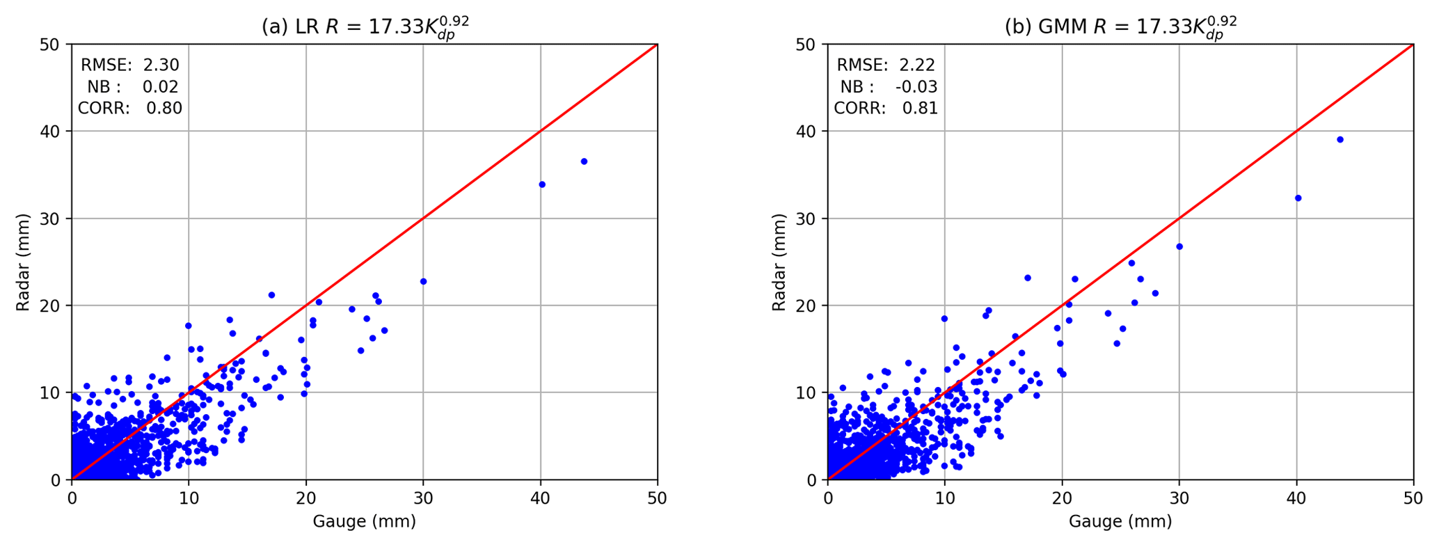
Figure 12 Same as Fig. 11 but for the optimal R–K_dp relation for the four sites. (a) LR R(K_dp) and (b) GMM R(K_dp).

Consistent with the data in Table 1, the rainfall at the four sites is predominately made up of light rain with hourly rain amounts no more than 2.5 mm h⁻¹. Nevertheless, according to Fig. 11, moderate rain with amounts between 2.6 and 8 mm h⁻¹ provides a considerable contribution to the total rain events, followed by a small portion of heavy rain with amounts more than 8 mm h⁻¹. When we study the scatterplots and statistics for each of the four sites, it is apparent that Bradford (Fig. 11a and b) and Sanborn (Fig. 11c and d) are more concentrated on the red line than Auxvasse (Fig. 11e and f) and Williamsburg (Fig. 11g and h), since Bradford and Sanborn are closer to the radar. Accordingly, RMSEs for Bradford and Sanborn (Table 2) are relatively small, about 13 %–35 % lower than Auxvasse and Williamsburg. Furthermore, it can be seen that Bradford and Sanborn show negative bias associated with negative NBs, indicating an underestimation of rain amounts by GMM K_dp. In contrast, a slight overestimation may be concluded for Auxvasse and Williamsburg by considering the point trends and the positive NBs. Additionally, Sanborn claims the highest ρ_RG out of the four sites, yielding the best consistency between the radar and gauge.

When compared to LR statistics as given in Table 2, it is clear that GMM improves the RMSEs, NBs and ρ_RG for Auxvasse and Williamsburg. Notably, the GMM-based NB for Auxvasse reaches a very small value of 0.04, one-fifth of LR-based NB. For Bradford, RMSE is reduced by GMM, but the absolute value of NB is slightly increased, while ρ_RG remains the same. On the other hand, for Sanborn, the GMM-based RMSE has been increased and the GMM-based NB and ρ_hv have been decreased comparing to the LR ones. It may be due to the local complex terrain near the radar. However, the difference of RMSE, NB, and ρ_hv between GMM and LR is a few hundredths of a millimeter, which is not significant relative to their absolute values. Overall, the rainfall estimates of GMM K_dp give a better performance than that of LR in terms of RMSE, NB, and ρ_RG at the far ranges.

To improve the accuracy of the radar rainfall estimation, we have optimized the R–K_dp relation in terms of the RMSE using the radar–gauge dataset. It leads to the relation as

$$\begin{array}{}\text{(37)}& R\left(K_{\mathrm{dp}}\right)=\mathrm{17.33}{K}_{\mathrm{dp}}^{\mathrm{0.92}}.\end{array}$$

Figure 12 shows the scatterplots of the radar–gauge data and the statistics of RMSE, NB, and ρ_RG obtained by Eq. (37) for all the four sites. It is clear that Eq. (37) has improved the negative trend in Eq. (33). As illustrated in Fig. 12a and b, the points give a better concentration on the one-to-one reference line with noticeable changes for higher R(K_dp). In Fig. 12a, the LR R(K_dp) achieves fairly good RMSE, NB, and ρ_RG values at 2.30, 0.02, and 0.80, respectively. On the other hand, the GMM R(K_dp) presents a similar distribution to the LR R(K_dp), but the points in Fig. 12b are shifted toward the vertical axis. Moreover, the GMM R(K_dp) gives better RMSE and ρ_RG at 2.22 and 0.81, respectively, and slightly worse NB at −0.03.

It can be found that the rain rates based on the GMM K_dp have a moderate consistency with the rain gauge data. To further improve the results, some advanced rain rate algorithms can be considered, such as the rain–ice separation technique in the IFloodS campaign (Chen et al., 2017b) and the radar–gauge comparison method in the MC3E campaign (Giangrande et al., 2014). Nevertheless, the GMM has the advantage over the existing methods, since it can yield the variance of K_dp. Furthermore, the variance of R can also be obtained by the K_dp mean and the K_dp variance via the R–K_dp relation, leading to the variability in the error characteristics of R. Thus, the variances can be used to study the streamflow trends in the hydrological model.

6 Summary and discussions

In this study, we proposed a probabilistic method based on the Gaussian mixture model to estimate the specific differential phase K_dp, which is the range derivative of the differential phase shift Φ_dp. The Gaussian mixture method (GMM) not only obtained the expected values of K_dp by differentiating the conditional expectation of Φ_dp, but also yielded the variance σ²(K_dp) regarding the errors in the calculation of the first derivative of Φ_dp.

As an initial step of GMM, the data masking was performed to eliminate the residual clutter in the measurements of the total differential phase (Ψ_dp). The data of r and Ψ_dp were first fitted into a simplified Gaussian mixture to generate a number of clusters, which were validated against the two sets of the σ(Ψ_dp) and σ(Ψ_dp)∕σ(r) thresholds given by radar reflectivity Z_H. The clusters were then combined to form the rain cell segments, and the segments were classified by comparing the weight accumulations of weather and clutter clusters. Next, the clusters within each segment were reevaluated by the thresholds according to the segment types. Finally, the azimuthally isolated points were masked out.

Secondly, the joint probability density function (PDF) was obtained by fitting the data of r and Ψ_dp into a mixture model with full covariance, where the cluster number m, weight w, mean μ, and covariance Σ were optimized via the expectation–maximization (EM) algorithm. Subsequently, the PDF of Ψ_dp conditioned on r was also a mixture with parameters related to the joint PDF. Finally, the Ψ_dp mean was estimated by the conditional expectation, and the statistical errors σ²(Ψ_dp) were given by the conditional variance, which was not always constant but varied with w and the marginal PDF of r.

Thirdly, the ambiguous Ψ_dp and backscattering differential phase shift δ_co were corrected by examining the two adjacent density ellipses in the mixture. On the one hand, if the former density ellipse had a mean larger than the latter one by 80^∘, the latter mean was added to 180^∘ for Ψ_dp unfolding. On the other hand, if the former mean was smaller than the latter one by 85^∘, the latter density ellipse was removed as δ_co. Moreover, for δ_co elimination, the first density ellipse mean was assumed to be below 90^∘, while the density ellipses with small weights were also removed.

Fourthly, the joint PDF of r and Φ_dp was used in the calculations of K_dp and σ²(K_dp). Since K_dp was the range derivative of Φ_dp, the expected values of K_dp were then obtained via the derivative of the expected value of Φ_dp. Moreover, by taking the first-order Taylor series expansion, σ²(K_dp) was the product of the square of the first derivative of K_dp and σ²(Φ_dp), yielding nonconstant values of σ²(K_dp).

In the final step, the expected values of K_dp were smoothed to reduce the associated σ²(K_dp). An FIR filter was implemented and iteratively applied to the data to search for an optimal window length. Subsequently, the reduced σ²(K_dp) was obtained by the sum of the original σ²(K_dp) weighted by the FIR coefficient squares within the window. Additionally, new Φ_dp were reconstructed from the smoothed K_dp, while σ²(Φ_dp) was also reduced.

The experimental results with a severe storm observed by the X-band polarimetric radar in the University of Missouri (MZZU) revealed the advantages of GMM. By studying the structure and evolution of a bow echo in the storm, it was concluded that the GMM K_dp was consistent with the gradients of raw Φ_dp along the leading edge of the bow echo, while large σ²(K_dp) values occurred with high variation of K_dp. The GMM method produced results similar to the LR method, with the ability to handle the missing data. Moreover, the hourly rain amounts based on K_dp were compared to the rain gauge data, showing fairly good agreement between radar and gauge measurements. The rain amounts obtained by GMM K_dp gave improvements over the linear regression model, particularly for the far ranges.

The potential applications of GMM K_dp and σ²(K_dp) include quantitative precipitation estimation (Cifelli et al., 2011; Chen et al., 2017a) and attenuation correction (Park et al., 2005a). For quantitative precipitation estimation, the relationship between K_dp and rain rate R is almost linear, since K_dp is about the fourth-order moment of the raindrop size distribution, and R is the 3.67th-order moment. As illustrated in Figs. 11 and 12, the R(K_dp) algorithm is consistent with the in situ measurements. To further investigate the R errors, it is necessary to consider the K_dp errors in the calculation of the first derivative of Φ_dp. The standard deviation σ(K_dp) is then related to σ(R) by a factor of R∕K_dp (Bringi and Chandrasekar, 2001). In a similar manner, K_dp is linearly proportional to the specific attenuation A_H and specific differential attenuation A_DP (Bringi and Hendry, 1990). Therefore, the errors of radar reflectivity Z_H and differential reflectivity Z_DR may also be proportional to σ(K_dp) after the attenuation correction and eventually contribute to the R errors via R(Z_H) and R(Z_H,Z_DR). Moreover, the error estimates can be used to study the propagation of uncertainty in the weather model and provide streamflow trends in the hydrological model. In the future study, the algorithm will also be extended to other frequencies, such as the C band (Vulpiani et al., 2012; May et al., 1999) and S band (Bringi and Chandrasekar, 2001). The thresholds in the data masking, the Ψ_dp unfolding, and the δ_co elimination will be adjusted according to the radar specifications. Nevertheless, the steps for the calculations of the PDFs of Ψ_dp and K_dp remain.

Appendix A: Regression-based estimation of K_dp

Let the total differential phase Ψ_dp be y, and let the range gate r be x. The Ψ_dp profile over small range segments can be approximated by a first-order polynomial; i.e.,

$$\begin{array}{}\text{(A1)}& y={\mathit{\beta }}_{\mathrm{0}}+{\mathit{\beta }}_{\mathrm{1}}x+\mathit{ϵ},\end{array}$$

where β₀ and β₁ are the coefficients in the linear approximation, and ϵ is an error function. It can be assumed that ϵ is independent and individually distributed with zero mean and variance of ${\mathit{\sigma }}_{\mathit{ϵ}}^{\mathrm{2}}={\mathit{\sigma }}^{\mathrm{2}}$.

In the linear regression, it is easy to find that

$$\begin{array}{}\text{(A2)}& {\mathit{\beta }}_{\mathrm{1}}={\displaystyle \frac{{\sum }_i(x_i-\stackrel{\mathrm{‾}}{x})(y_i-\stackrel{\mathrm{‾}}{y})}{{\sum }_i(x_i-\stackrel{\mathrm{‾}}{x}{)}^{\mathrm{2}}}},\end{array}$$

where $\stackrel{\mathrm{‾}}{x}$ and $\stackrel{\mathrm{‾}}{y}$ are the means of x and y in the segment, respectively. Since

$$\begin{array}{}\text{(A3)}& \sum _i(x_i-\stackrel{\mathrm{‾}}{x})(y_i-\stackrel{\mathrm{‾}}{y})=\sum _i(x_i-\stackrel{\mathrm{‾}}{x})y_i-\sum _i(x_i-\stackrel{\mathrm{‾}}{x})\stackrel{\mathrm{‾}}{y}\end{array}$$

and

$$\begin{array}{}\text{(A4)}& \sum _i(x_i-\stackrel{\mathrm{‾}}{x})\stackrel{\mathrm{‾}}{y}=\stackrel{\mathrm{‾}}{y}\left(\sum _i{x}_i-N\stackrel{\mathrm{‾}}{x}\right)=\stackrel{\mathrm{‾}}{y}(N\stackrel{\mathrm{‾}}{x}-N\stackrel{\mathrm{‾}}{x})=\mathrm{0},\end{array}$$

we have

$$\begin{array}{}\text{(A5)}& {\mathit{\beta }}_{\mathrm{1}}={\displaystyle \frac{{\sum }_i(x_i-\stackrel{\mathrm{‾}}{x})y_i}{{\sum }_i(x_i-\stackrel{\mathrm{‾}}{x}{)}^{\mathrm{2}}}},\end{array}$$

where N is the number of the gates in the segment.

It is noted that the range gate r is equally spaced with an interval of Δr, Ψ_dp is the two-way propagation phase shift, and K_dp is the one-way specific differential phase. The K_dp is then estimated by

$$\begin{array}{}\text{(A6)}& K_{\mathrm{dp}}={\displaystyle \frac{{\sum }_{i=\mathrm{1}}^n{\mathrm{\Psi }}_{\mathrm{dp}}\left(r_i\right)\left[\mathrm{6}i-\mathrm{3}(n+\mathrm{1})\mathrm{\Delta }r\right]}{n(n-\mathrm{1})(n+\mathrm{1})\mathrm{\Delta }{r}^{\mathrm{2}}}}.\end{array}$$

At the S band, the backscattering differential phase shift δ_co is often negligible, and thus Ψ_dp and Φ_dp are interchangeable, leading to Eq. (2).

By taking the variance on both sides of Eq. (A5) and noting ϵ is the only variable, we have

$$\begin{array}{}\text{(A7)}& {\displaystyle }{\mathit{\sigma }}^{\mathrm{2}}\left({\mathit{\beta }}_{\mathrm{1}}\right)& {\displaystyle }={\mathit{\sigma }}^{\mathrm{2}}\left({\displaystyle \frac{{\sum }_i(x_i-\stackrel{\mathrm{‾}}{x})({\mathit{\beta }}_{\mathrm{0}}+{\mathit{\beta }}_{\mathrm{1}}{x}_i+\mathit{ϵ})}{{\sum }_i(x_i-\stackrel{\mathrm{‾}}{x}{)}^{\mathrm{2}}}}\right),\text{(A8)}& {\displaystyle }& {\displaystyle }={\displaystyle \frac{{\sum }_i(x_i-\stackrel{\mathrm{‾}}{x}{)}^{\mathrm{2}}{\mathit{\sigma }}_{\mathit{ϵ}}^{\mathrm{2}}}{{\left[{\sum }_i(x_i-\stackrel{\mathrm{‾}}{x}{)}^{\mathrm{2}}\right]}^{\mathrm{2}}}},\text{(A9)}& {\displaystyle }& {\displaystyle }={\displaystyle \frac{{\mathit{\sigma }}^{\mathrm{2}}}{{\sum }_i(x_i-\stackrel{\mathrm{‾}}{x}{)}^{\mathrm{2}}}}.\end{array}$$

Similar to Eq. (A6), we have

$$\begin{array}{}\text{(A10)}& {\mathit{\sigma }}^{\mathrm{2}}\left(K_{\mathrm{dp}}\right)={\displaystyle \frac{\mathrm{3}{\mathit{\sigma }}^{\mathrm{2}}\left({\mathrm{\Psi }}_{\mathrm{dp}}\right)}{\mathrm{\Delta }{r}^{\mathrm{2}}\left[n(n-\mathrm{1})(n+\mathrm{1})\right]}}.\mathit{\#}\end{array}$$

Appendix B: Variance of Φ_dp

We consider the range r as an independent variable, denoted as x, and Φ_dp as a dependent variable, denoted as y. The joint distribution of $\mathit{z}=(x,y)$ follows a Gaussian mixture as

$$\begin{array}{}\text{(B1)}& p\left(\mathit{z}\right)=\sum _{i=\mathrm{1}}^m{w}_i\mathcal{N}(\mathit{z};{\mathit{\mu }}_i,{\mathbf{\Sigma }}_i),\end{array}$$

where w_i, μ_i, and Σ_i are the weight, mean, and covariance for each component, respectively. The probability of y conditioned on x is also a Gaussian mixture with parameters $w_i^{y|x}$, ${\mathit{\mu }}_i^{y|x}$, and ${\mathrm{\Sigma }}_i^{y|x}$, leading to the conditional expectation as

$$\begin{array}{}\text{(B2)}& {\displaystyle }E\left(y\right|x)& {\displaystyle }=\int y\sum _{i=\mathrm{1}}^m{w}_i^{y|x}\mathcal{N}\left(y;{\mathit{\mu }}_i^{y|x},{\mathrm{\Sigma }}_i^{y|x}\right)\mathrm{d}y,\text{(B3)}& {\displaystyle }& {\displaystyle }=\sum _{i=\mathrm{1}}^m{w}_i^{y|x}\int y\mathcal{N}\left(y;{\mathit{\mu }}_i^{y|x},{\mathrm{\Sigma }}_i^{y|x}\right)\mathrm{d}y,\text{(B4)}& {\displaystyle }& {\displaystyle }=\sum _{i=\mathrm{1}}^m{w}_i{\mathit{\mu }}_i^{y|x},\end{array}$$

and the second-order moment as

$$\begin{array}{}\text{(B5)}& {\displaystyle }E\left(y^{\mathrm{2}}\right|x)& {\displaystyle }=\int y^{\mathrm{2}}\sum _{i=\mathrm{1}}^m{w}_i^{y|x}\mathcal{N}\left(y;{\mathit{\mu }}_i^{y|x},{\mathrm{\Sigma }}_i^{y|x}\right)\mathrm{d}y,\text{(B6)}& {\displaystyle }& {\displaystyle }=\sum _{i=\mathrm{1}}^m{w}_i^{y|x}\int y^{\mathrm{2}}\mathcal{N}\left(y;{\mathit{\mu }}_i^{y|x},{\mathrm{\Sigma }}_i^{y|x}\right)\mathrm{d}y,\text{(B7)}& {\displaystyle }& {\displaystyle }=\sum _{i=\mathrm{1}}^m{w}_i^{y|x}\left[{\mathrm{\Sigma }}_i^{y|x}+{\left({\mathit{\mu }}_i^{y|x}\right)}^{\mathrm{2}}\right].\end{array}$$

Therefore, the conditional variance is expressed as

$$\begin{array}{}\text{(B8)}& {\displaystyle }{\mathit{\sigma }}^{\mathrm{2}}\left(y\right|x)=E(y^{\mathrm{2}}\left|x\right)-{\left[E\left(y\right|x)\right]}^{\mathrm{2}},\text{(B9)}& {\displaystyle }\begin{array}{rl}& =\sum _{i=\mathrm{1}}^m{w}_i^{y|x}\left[{\mathrm{\Sigma }}_i^{y|x}+{\left({\mathit{\mu }}_i^{y|x}\right)}^{\mathrm{2}}\right]\\ & -{\left(\sum _{i=\mathrm{1}}^m{w}_i^{y|x}{\mathit{\mu }}_i^{y|x}\right)}^{\mathrm{2}}.\mathit{\#}\end{array}\end{array}$$

Appendix C: Conditional expectation of K_dp

First, we need to show that the derivative of the expected value of random variable y as a function of random variable x is equal to the expected value of the derivative of the expected value of y. By the definition, the derivative of y is expressed as

$$\begin{array}{}\text{(C1)}& {\displaystyle }{E}^{\prime }\left[y\right(x\left)\right]& {\displaystyle }=\underset{h\to \mathrm{0}}{lim}{\displaystyle \frac{\mathrm{1}}{h}}\left\{E\left[y\right(x+h\left)\right]-E\left[y\right(x\left)\right]\right\},\text{(C2)}& {\displaystyle }& {\displaystyle }=\underset{h\to \mathrm{0}}{lim}E\left[{\displaystyle \frac{y(x+h)-y\left(x\right)}{h}}\right],\text{(C3)}& {\displaystyle }& {\displaystyle }=\underset{h\to \mathrm{0}}{lim}E\left\{y^{\prime }\left[\mathit{\tau }\right(h\left)\right]\right\},\end{array}$$

where $\mathit{\tau }\left(h\right)\in (x,x+h)$ exists by the mean value theorem. By assuming $\left|y^{\prime }\left[\mathit{\tau }\right(h\left)\right]\right|\le Z$, we can use the dominated convergence theorem to obtain

$$\begin{array}{}\text{(C4)}& {\displaystyle }{E}^{\prime }\left[y\right(x\left)\right]& {\displaystyle }=E\left\{\underset{h\to \mathrm{0}}{lim}{y}^{\prime }\left[\mathit{\tau }\right(h\left)\right]\right\},\text{(C5)}& {\displaystyle }& {\displaystyle }=E\left[y^{\prime }\left(x\right)\right].\end{array}$$

According to the conclusion in Eq. (C5), the expected value of y^′ is expressed as

$$\begin{array}{}\text{(C6)}& E\left(y^{\prime }\right|x)=E^{\prime }(y\left|x\right)=\sum _{i=\mathrm{1}}^m{w}_i^{y|x}{\left({\mathit{\mu }}_i^{y|x}\right)}^{\prime }+\sum _{i=\mathrm{1}}^m{\left(w_i^{y|x}\right)}^{\prime }{\mathit{\mu }}_i^{y|x}.\end{array}$$

Since ${\left({\mathit{\mu }}_i^{y|x}\right)}^{\prime }=a_i$ and $w_i^{y|x}=\frac{f_i\left(x\right)}{f\left(x\right)}$, the first term is equal to

$$\begin{array}{}\text{(C7)}& \sum _{i=\mathrm{1}}^m{w}_i^{y|x}{\left({\mathit{\mu }}_i^{y|x}\right)}^{\prime }=\sum _{i=\mathrm{1}}^m{a}_i{\displaystyle \frac{f_i\left(x\right)}{f\left(x\right)}}.\end{array}$$

Meanwhile, the second term is given as

$$\begin{array}{}\text{(C8)}& \begin{array}{rlr}\sum _{i=\mathrm{1}}& {}^m{\left(w_i^{y|x}\right)}^{\prime }{\mathit{\mu }}_i^{y|x}& =\sum _{i=\mathrm{1}}^m{\displaystyle \frac{f_i^{\prime }\left(x\right)f\left(x\right)-f_i\left(x\right)f^{\prime }\left(x\right)}{f^{\mathrm{2}}\left(x\right)}}\\ & (a_{i}x+b_i).\end{array}\end{array}$$

Based on the properties of the Gaussian function, the derivatives of f_i(x) and f(x) are expressed as

$$\begin{array}{}\text{(C9)}& {\displaystyle }{f}_i^{\prime }\left(x\right)& {\displaystyle }=-{\displaystyle \frac{x-{\mathit{\mu }}_i^x}{{\mathrm{\Sigma }}_i^{xx}}}{f}_i\left(x\right)\text{and}\text{(C10)}& {\displaystyle }{f}^{\prime }\left(x\right)& {\displaystyle }=-\sum _{j=\mathrm{1}}^m{\displaystyle \frac{x-{\mathit{\mu }}_j^x}{{\mathrm{\Sigma }}_j^{xx}}}{f}_j\left(x\right).\end{array}$$

By substituting Eqs. (C9) and (C10) into Eq. (C8), the second term is transformed as

$$\begin{array}{}\text{(C11)}& \begin{array}{rl}\sum _{i=\mathrm{1}}& {}^m{\left(w_i^{y|x}\right)}^{\prime }{\mathit{\mu }}_i^{y|x}={\displaystyle \frac{\mathrm{1}}{f^{\mathrm{2}}\left(x\right)}}\left[\sum _{i=\mathrm{1}}^m\sum _{j=\mathrm{1}}^m\right.\\ & \left.\left({\displaystyle \frac{x-{\mathit{\mu }}_j^x}{{\mathrm{\Sigma }}_j^{xx}}}-{\displaystyle \frac{x-{\mathit{\mu }}_i^x}{{\mathrm{\Sigma }}_i^{xx}}}\right)f_i\left(x\right)f_j\left(x\right)(a_{i}x+b_i)\right].\end{array}\end{array}$$

By substituting Eqs. (C7) and (C11) into Eq. (C6), we obtain

$$\begin{array}{}\text{(C12)}& \begin{array}{rl}& E\left(\left.y^{\prime }\right|x\right)={\displaystyle \frac{\mathrm{1}}{f^{\mathrm{2}}\left(x\right)}}\left\{\sum _{i=\mathrm{1}}^m\sum _{j=\mathrm{1}}^m{f}_i\left(x\right)f_j\left(x\right)\right.\\ & \left.\left[\left({\displaystyle \frac{x-{\mathit{\mu }}_j^x}{{\mathrm{\Sigma }}_j^{xx}}}-{\displaystyle \frac{x-{\mathit{\mu }}_i^x}{{\mathrm{\Sigma }}_i^{xx}}}\right)(a_{i}x+b_i)+a_i\right]\right\}\mathit{\#}.\end{array}\end{array}$$

Appendix D: Variance of K_dp

The first-order Taylor expansion is defined as

$$\begin{array}{}\text{(D1)}& g\left(y\right)=g\left(\mathit{\theta }\right)+g^{\prime }\left(\mathit{\theta }\right)(y-\mathit{\theta })+\mathit{ϵ},\end{array}$$

where θ=E(y) is the mean of random variable y, and ϵ is the sum of the higher-order Taylor series. By considering the conclusion in Eq. (C5), it can be noted that the expected values of the coefficients associated with the derivatives in Eq. (D1) are zeros if the series is expanded at the mean value of y. By taking mathematical expectations on both sides of Eq. (D1), it is transformed as

$$\begin{array}{}\text{(D2)}& {\displaystyle }E\left[g\right(y\left)\right]& {\displaystyle }\approx g\left(\mathit{\theta }\right)+g^{\prime }\left(\mathit{\theta }\right)\left[E\right(y)-\mathit{\theta }],\text{(D3)}& {\displaystyle }& {\displaystyle }=g\left(\mathit{\theta }\right).\end{array}$$

From Eqs. (D1) and (D3), the variance of g(y) is approximated as

$$\begin{array}{}\text{(D4)}& {\displaystyle }{\mathit{\sigma }}^{\mathrm{2}}\left[g\right(y\left)\right]& {\displaystyle }\approx E\left\{\left[g\right(y)-g(\mathit{\theta }){]}^{\mathrm{2}}\right\},\text{(D5)}& {\displaystyle }& {\displaystyle }\approx E\left\{\left[g^{\prime }\right(\mathit{\theta }\left)\right(y-\mathit{\theta }){]}^{\mathrm{2}}\right\},\text{(D6)}& {\displaystyle }& {\displaystyle }=g^{\prime }\left(\mathit{\theta }{)}^{\mathrm{2}}{\mathit{\sigma }}^{\mathrm{2}}\right(y).\end{array}$$

Let g(y) be y^′, and then we have

$$\begin{array}{}\text{(D7)}& {\mathit{\sigma }}^{\mathrm{2}}\left(y^{\prime }\right|x)=[E^{\prime \prime }\left(y\right|x\left){]}^{\mathrm{2}}{\mathit{\sigma }}^{\mathrm{2}}\right(y\left|x\right).\end{array}$$

From Eq. (B9), we can see that

$$\begin{array}{}\text{(D8)}& \begin{array}{rl}{\mathit{\sigma }}^{\mathrm{2}}\left(y\right|x)& =\sum _{i=\mathrm{1}}^m{w}_i^{y|x}{\mathrm{\Sigma }}_i^{y|x}+\sum _{i=\mathrm{1}}^m{w}_i^{y|x}{\left({\mathit{\mu }}_i^{y|x}\right)}^{\mathrm{2}}\\ & -{\left(\sum _{i=\mathrm{1}}^m{w}_i^{y|x}{\mathit{\mu }}_i^{y|x}\right)}^{\mathrm{2}}.\end{array}\end{array}$$

By taking the derivative of Eq. (C6), the second derivative of the expected value of y conditioned on x becomes

$$\begin{array}{}\text{(D9)}& {\displaystyle }\begin{array}{rl}{E}^{\prime \prime }\left(y\right|x)& =\sum _{i=\mathrm{1}}^m{w}_i^{y|x}({\mathit{\mu }}_i^{y|x}{)}^{\prime \prime }+\mathrm{2}\sum _{i=\mathrm{1}}^m({\mathit{\mu }}_i^{y|x}{)}^{\prime }(w_i^{y|x}{)}^{\prime }\\ & +\sum _{i=\mathrm{1}}^m{\mathit{\mu }}_i^{y|x}(w_i^{y|x}{)}^{\prime \prime },\end{array}\text{(D10)}& {\displaystyle }=\mathrm{2}\sum _{i=\mathrm{1}}^m{a}_i(w_i^{y|x}{)}^{\prime }+\sum _{i=\mathrm{1}}^m(a_{i}x+b_i\left)\right(w_i^{y|x}{)}^{\prime \prime },\end{array}$$

since $({\mathit{\mu }}_i^{y|x}{)}^{\prime }=a_i$ and $({\mathit{\mu }}_i^{y|x}{)}^{\prime \prime }=\mathrm{0}$. From Eq. (C8), the first derivative of the weighting function in the conditional probability is

$$\begin{array}{}\text{(D11)}& {\left(w_i^{y|x}\right)}^{\prime }={\displaystyle \frac{\mathrm{1}}{f^{\mathrm{2}}\left(x\right)}}\sum _{j=\mathrm{1}}^m{f}_j\left(x\right)f_i\left(x\right)\left({\displaystyle \frac{x-{\mathit{\mu }}_j^x}{{\mathrm{\Sigma }}_j^{xx}}}-{\displaystyle \frac{x-{\mathit{\mu }}_i^x}{{\mathrm{\Sigma }}_i^{xx}}}\right).\end{array}$$

Let g_i(x) be the summation term. The second derivative is then expressed as

$$\begin{array}{}\text{(D12)}& {\displaystyle }{\left(w_i^{y|x}\right)}^{\prime \prime }& {\displaystyle }={\displaystyle \frac{g_i^{\prime }\left(x\right)f\left(x\right)-\mathrm{2}{f}^{\prime }\left(x\right)g_i\left(x\right)}{f^{\mathrm{3}}\left(x\right)}},\text{where}\text{(D13)}& {\displaystyle }{g}_i\left(x\right)& {\displaystyle }=\sum _{j=\mathrm{1}}^m{f}_j\left(x\right)f_i\left(x\right)\left({\displaystyle \frac{x-{\mathit{\mu }}_j^x}{{\mathrm{\Sigma }}_j^{xx}}}-{\displaystyle \frac{x-{\mathit{\mu }}_i^x}{{\mathrm{\Sigma }}_i^{xx}}}\right).\end{array}$$

According to the properties of the Gaussian mixture, the first derivative of the marginal distribution of x is

$$\begin{array}{}\text{(D14)}& f^{\prime }\left(x\right)=-\sum _{j=\mathrm{1}}^m\left({\displaystyle \frac{x-{\mathit{\mu }}_j}{{\mathrm{\Sigma }}_j}}\right)f_j\left(x\right).\end{array}$$

Similarly, the first derivative of g(x) if given as

$$\begin{array}{}\text{(D15)}& {\displaystyle }\begin{array}{rl}& g_i^{\prime }\left(x\right)=\sum _{j=\mathrm{1}}^m\left[-{\displaystyle \frac{x-{\mathit{\mu }}_j^x}{{\mathrm{\Sigma }}_j^{xx}}}\left({\displaystyle \frac{x-{\mathit{\mu }}_j^x}{{\mathrm{\Sigma }}_j^{xx}}}-{\displaystyle \frac{x-{\mathit{\mu }}_i^x}{{\mathrm{\Sigma }}_i^{xx}}}\right)f_j\left(x\right)\right.f_i\left(x\right)\\ & -{\displaystyle \frac{x-{\mathit{\mu }}_i^x}{{\mathrm{\Sigma }}_i^{xx}}}\left({\displaystyle \frac{x-{\mathit{\mu }}_j^x}{{\mathrm{\Sigma }}_j^{xx}}}-{\displaystyle \frac{x-{\mathit{\mu }}_i^x}{{\mathrm{\Sigma }}_i^{xx}}}\right)f_j\left(x\right)f_i\left(x\right)\\ & \left.+\left({\displaystyle \frac{\mathrm{1}}{{\mathrm{\Sigma }}_j^{xx}}}-{\displaystyle \frac{\mathrm{1}}{{\mathrm{\Sigma }}_i^{xx}}}\right)f_j\left(x\right)f_i\left(x\right)\right],\end{array}\text{(D16)}& {\displaystyle }\begin{array}{rl}& =\sum _{j=\mathrm{1}}^m\left[\left({\displaystyle \frac{x-{\mathit{\mu }}_i^x}{{\mathrm{\Sigma }}_i^{xx}}}-{\displaystyle \frac{x-{\mathit{\mu }}_j^x}{{\mathrm{\Sigma }}_j^{xx}}}\right)\left({\displaystyle \frac{x-{\mathit{\mu }}_i^x}{{\mathrm{\Sigma }}_i^{xx}}}+{\displaystyle \frac{x-{\mathit{\mu }}_j^x}{{\mathrm{\Sigma }}_j^{xx}}}\right)\right.\\ & \left.f_j\left(x\right)f_i\left(x\right)+\left({\displaystyle \frac{\mathrm{1}}{{\mathrm{\Sigma }}_j^{xx}}}-{\displaystyle \frac{\mathrm{1}}{{\mathrm{\Sigma }}_i^{xx}}}\right)f_j\left(x\right)f_i\left(x\right)\right],\end{array}\text{(D17)}& {\displaystyle }\begin{array}{rl}& =\sum _{j=\mathrm{1}}^m\left[{\left({\displaystyle \frac{x-{\mathit{\mu }}_i^x}{{\mathrm{\Sigma }}_i^{xx}}}\right)}^{\mathrm{2}}-{\left({\displaystyle \frac{x-{\mathit{\mu }}_j^x}{{\mathrm{\Sigma }}_j^{xx}}}\right)}^{\mathrm{2}}\right]f_j\left(x\right)f_i\left(x\right)\\ & +\left({\displaystyle \frac{\mathrm{1}}{{\mathrm{\Sigma }}_j^{xx}}}-{\displaystyle \frac{\mathrm{1}}{{\mathrm{\Sigma }}_i^{xx}}}\right)f_j\left(x\right)f_i\left(x\right),\end{array}\text{(D18)}& {\displaystyle }\begin{array}{rl}& =\sum _{j=\mathrm{1}}^m{f}_j\left(x\right)f_i\left(x\right)\left[{\left({\displaystyle \frac{x-{\mathit{\mu }}_i^x}{{\mathrm{\Sigma }}_i^{xx}}}\right)}^{\mathrm{2}}-{\left({\displaystyle \frac{x-{\mathit{\mu }}_j^x}{{\mathrm{\Sigma }}_j^{xx}}}\right)}^{\mathrm{2}}\right.\\ & \left.+{\displaystyle \frac{\mathrm{1}}{{\mathrm{\Sigma }}_j^{xx}}}-{\displaystyle \frac{\mathrm{1}}{{\mathrm{\Sigma }}_i^{xx}}}\right].\mathit{\#}\end{array}\end{array}$$