Characterisation of the filter inlet system on the FAAM BAe-146 research aircraft and its use for size-resolved aerosol composition measurements

Atmospheric aerosol particles are important for our planet's climate because they interact with radiation and clouds. Hence, having characterised methods to collect aerosol from aircraft for detailed offline analysis are valuable. However, collecting aerosol, particularly coarse-mode aerosol, onto substrates from a fast-moving aircraft is challenging and can result in both losses and enhancement in particles. Here we present the characterisation of an inlet system designed for collection of aerosol onto filters on board the Facility for Airborne Atmospheric Measurements (FAAM) BAe-146-301 Atmospheric Research Aircraft. We also present an offline scanning electron microscopy (SEM) technique for quantifying both the size distribution and size-resolved composition of the collected aerosol. We use this SEM technique in parallel with online underwing optical probes in order to experimentally characterise the efficiency of the inlet system. We find that the coarse-mode aerosol is sub-isokinetically enhanced, with a peak enhancement at around 10 µm up to a factor of 2 under recommended operating conditions. Calculations show that the efficiency of collection then decreases rapidly at larger sizes. In order to minimise the isokinetic enhancement of coarse-mode aerosol, we recommend sampling with total flow rates above 50 L min⁻¹; operating the inlet with the bypass fully open helps achieve this by increasing the flow rate through the inlet nozzle. With the inlet characterised, we also present single-particle chemical information obtained from X-ray spectroscopy analysis, which allows us to group the particles into composition categories.

1 Introduction

Atmospheric aerosol particles are known to have an important effect on climate through directly scattering or absorbing solar and terrestrial radiation as well as through indirect effects such as acting as cloud condensation nuclei (CCN) or ice-nucleating particles (INPs) (Albrecht, 1989; DeMott et al., 2010; Haywood and Boucher, 2000; Hoose and Möhler, 2012; Lohmann and Diehl, 2006; Lohmann and Gasparini, 2017). Aerosol particles across the fine (diameter < 2 µm) and coarse (> 2 µm) modes are important for these atmospheric processes. For example, aerosol in the accumulation mode acts as CCN (Seinfeld and Pandis, 2006), whereas supermicron particles are thought to contribute substantially to the INP population (Creamean et al., 2018; Mason et al., 2016; Pruppacher and Klett, 1997). Hence, being able to sample across the fine and coarse modes is required to understand the role aerosol plays in our atmosphere. However, sampling aerosol particles without biases can be challenging, this being especially so on a fast-moving aircraft (Baumgardner et al., 2011; Baumgardner and Huebert, 1993; McMurry, 2000; Wendisch and Brenguier, 2013).

It is necessary to sample aerosol from aircraft because in many cases aircraft offer the only opportunity to study aerosol and aerosol–cloud interactions at cloud-relevant altitudes (Wendisch and Brenguier, 2013). However, the relatively high speeds involved present a set of unique challenges for sampling aerosol particles. This is especially so for coarse-mode aerosols, which are prone to both losses as well as enhancements because their high inertia inhibits their ability to follow the air streamlines when they are distorted by the aircraft fuselage and the inlet (Brockmann, 2011; McMurry, 2000; von der Weiden et al., 2009). Therefore, inlet design and characterisation become extremely important when sampling aerosol particles.

In this study we characterise the inlet system used for collecting filter samples (known as the filter system) on board the UK's FAAM BAe-146-301 Atmospheric Research Aircraft. This system has been used for many years, but its characterisation has been limited (Chou et al., 2008; Price et al., 2018; Ryder et al., 2018; Young et al., 2016). Our goal in this characterisation work was to define recommendations for the use of the inlet system to minimise sampling biases and define the size limitation and the biases that exist. While the filter samples could be used for a variety of offline analyses, we have performed this characterisation with two specific goals in mind: firstly, we want to use this inlet system for quantification of INP (the technique for this analysis has been described previously (Price et al., 2018) and will not be further discussed here); secondly, we have adapted and developed a technique for quantification of and the size-resolved composition of the samples using scanning electron microscopy (SEM). We use this technique in order to test the inlet efficiency. These experiments are underpinned by calculations which elucidate how the biases are impacted by variables such as flow speed, angle of attack, and use of the bypass system. Finally we present an example of the use of the inlet for determining the size-resolved composition of an aerosol sample collected from the FAAM BAe-146. All data associated with this paper are available at https://doi.org/10.5518/724 (Sanchez-Marroquin et al., 2019).

2 Description and theoretical sampling characteristics of the filter inlet system on the Facility for Airborne Atmospheric Measurements (FAAM) aircraft

Ideally, aerosol particles would be sampled through inlets without enhancement or losses. However, this is typically not the case when sampling from aircraft; hence it is important to know how the size distribution of the aerosol particles is affected by the sampling. Generally, an aircraft moves at high velocities with respect to the air mass that is being sampled. During sampling on the FAAM BAe-146 the indicated airspeed is 100 m s⁻¹, which yields to a true airspeed that fluctuates between 100 and 120 m s⁻¹. The air mass has to decelerate when passing through the inlet (Baumgardner and Huebert, 1993) and this tends to result in inertial enhancement of coarse-mode aerosol. There are also losses through the inlet system, for example, through inertial impaction at bends or gravitational settling in horizontal sections of pipework. These inlet characteristics need to be considered if the subsequent analysis of the aerosol samples is to be quantitative. In this section we first describe the existing inlet system and then present theoretical calculations for the size-dependent losses and enhancements.

2.1 Description of the filter system

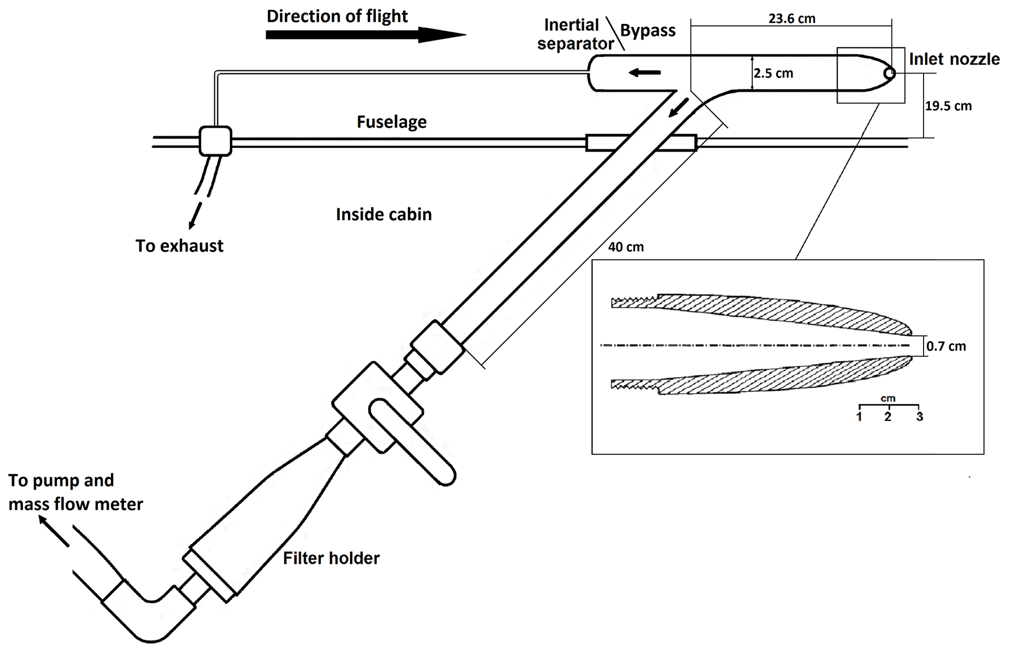
The FAAM BAe-146 has two identical inlets for sampling aerosol onto filters for offline analysis. This inlet system was used to sample aerosol particles on board the C-130 aircraft before being installed on the FAAM BAe-146 (Andreae et al., 1988; Andreae et al., 2000; Talbot et al., 1990), and it has been used to sample aerosol particles on the FAAM BAe-146 (e.g. Chou et al., 2008; Hand et al., 2010; Price et al., 2018; Young et al., 2016). A diagram of the inlet system can be seen in Fig. 1. The two parallel inlet and filter holder systems, which each have a nozzle whose curved leading edge profile follows the criteria for aircraft engine intakes at low Mach numbers (low speeds when compared with the speed of sound; for the FAAM BAe-146 during sampling this is ∼0.3), and it is designed to avoid the distortion of the pressure field at the end of the nozzle, flow separation, and turbulence (Andreae et al., 1988; Talbot et al., 1990). The inlet has a bypass to remove water droplets or ice crystals through inertial separation and also enhance the flow rate at the inlet nozzle (Talbot et al., 1990). The flow through the bypass (bypass flow) can be regulated using a valve and it is driven passively by the pressure differential between the ram pressure inlet and the Venturi effect on the exhaust. After turning inside the aircraft, the airstream containing the aerosol particles continues through the filter stack after passing a valve. The air flow through the filter (filter flow) is measured by a mass flow meter, which measures the sampled air mass and reports it in equivalent litres at standard conditions (273.15 K, 1013.529 hPa). The uncertainty for this flow meter is 1 % of the full scale (400 L min⁻¹). The effect of water vapour on the mass flow has not been corrected since its effect is negligible. The signal is integrated by an electronics unit to give the total volume of air sampled for any given time period. There is also a valve between the pump and the flow meter. The valve allows the inlet and pump to be isolated from the filter holder when changing the filter. The system uses a double-flow side channel vacuum pump model SAH55 made by Elmo Rietschle (Gardner Denver Inc.), aided by the ram effect of the aircraft. The flow rate at the inlet nozzle (total flow) is the sum of the bypass flow and the filter flow. The inlet nozzle is located at 19.5 cm of the aircraft fuselage, so the sampling is carried out in the free stream, outside the boundary layer.

Figure 1 Schematic diagram of one of the two parallel lines of the filter inlet system.

2.2 Sampling efficiency

We present theoretical estimates of the losses and enhancements due to aspiration, inlet inertial deposition, turbulent inertial deposition, inertial deposition in bends, and gravitational effects in Fig. 2a. We used the term “efficiency” to define the ratio between the number concentrations of particles after they were perturbed relative to the unperturbed value. If the efficiency is above 1, the number of particles is enhanced, whereas if it is below 1 particles are lost before they reach the filter.

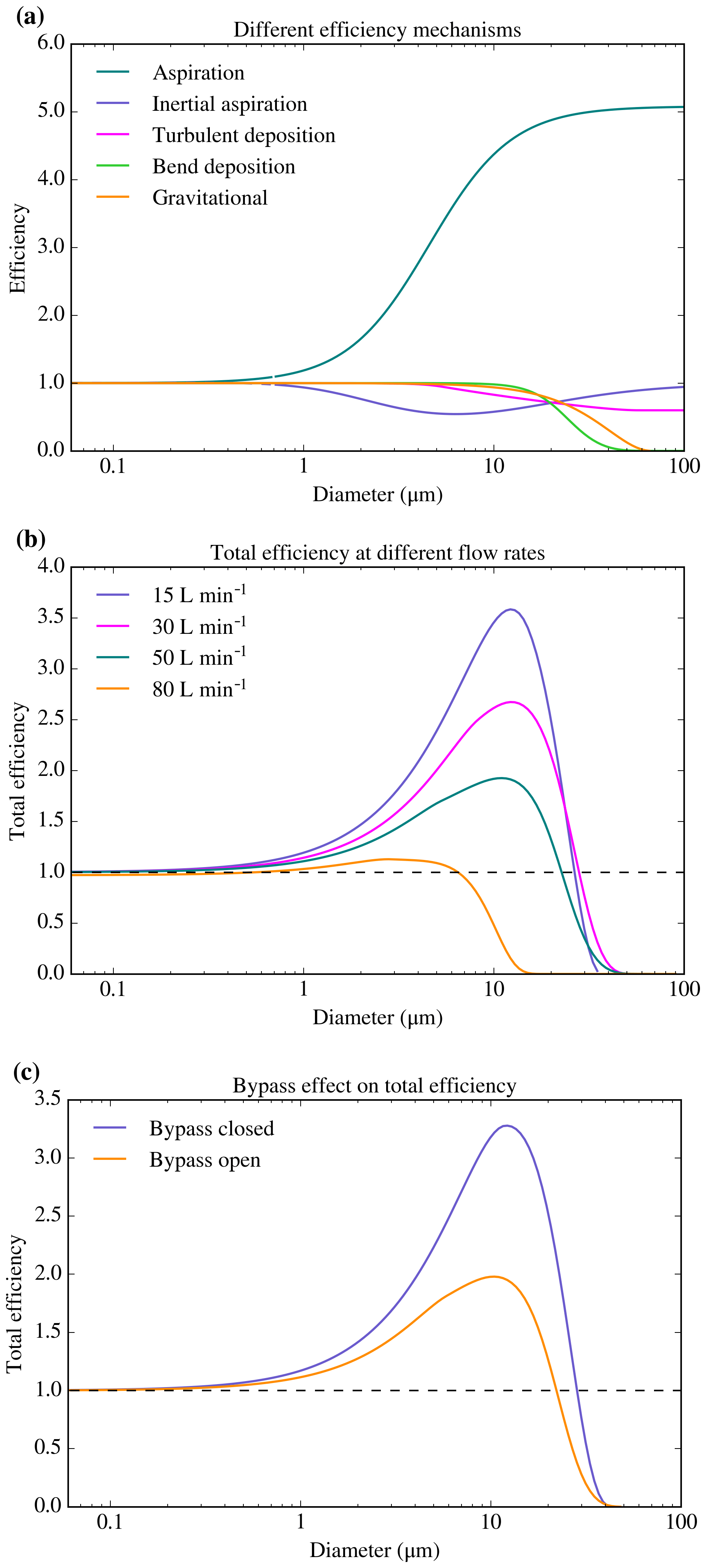
Figure 2 Theoretical efficiencies of the filter inlet system. (a) Efficiencies of the four mechanisms considered in this work for a total flow rate of 50 L min⁻¹. We have assumed a dynamic viscosity of $\mathrm{1.82}\times {\mathrm{10}}^{-\mathrm{5}}$ kg m⁻¹ s⁻¹ (value for 0 ^∘C) and a particle density of 1000 kg m⁻³. The speed of the air mass (U₀) was 110 m s⁻¹, a typical FAAM BAe-146 flying speed at low altitudes. (b) Total efficiency for four different total flow rates. For the 80 L min⁻¹ case, turbulent deposition through the whole line was considered since the flow was turbulent through the whole pipe. (c) Total efficiency considering all the described mechanisms for a 20 L min⁻¹ filter flow rate with the bypass closed and a 20 L min⁻¹ filter flow rate with the bypass open (considering a bypass flow of 25 L min⁻¹).

The sampling efficiency of any inlet depends on the flow rates and the flow regime (laminar vs. turbulent), the pressure, and the temperature. Filter flow rates for 0.4 µm polycarbonate filters normally vary between 10 and 50 L min⁻¹ depending on altitude (see Sect. 2.3 for a discussion of flow rates). The bypass flow rate (when it is fully open) can go up to 35 L min⁻¹ at 30 m and 22 L min⁻¹ at 6 km (volumetric litres at standard conditions: 273.15 K, 1013.529 hPa), but it is not measured routinely. In the 2.5 cm diameter section of the inlet, just after the inlet nozzle, the Reynolds number (Re) is below the turbulent regime threshold (Re > 4000) for flow rates below 65 L min⁻¹. For larger values of Re, the flow starts becoming turbulent. At the inlet nozzle, where the diameter is 0.7 cm, Re is above 4000 for flow rates above 20 L min⁻¹, so the flow is briefly in the turbulent regime at the inlet for most sampling conditions. Fully characterising the losses and enhancements of aerosol particles passing through the inlet is very challenging since there are several aerosol size-dependent mechanisms that can enhance or diminish the number of aerosol particles that arrive at the filter.

Here we have considered the most important of these mechanisms (von der Weiden et al., 2009) in order to estimate the inlet efficiency (see Fig. 2a) for a total flow rate of 50 L min⁻¹ (all the flow rates of our calculations are given in litres per minute at standard conditions: 273.15 K, 1013.529 hPa). These loss mechanisms and their importance in this inlet system are defined as follows (a discussion on the choice of equations, how they have been applied, and the excluded mechanisms can be found in Appendix A).

Aspiration efficiency has been calculated using the empirical equation as developed in Belyaev and Levin (1972) and Belyaev and Levin (1974). As one can see in Fig. 2a this mechanism enhances aerosol particles, tending to 1 for small diameters and to the ratio in between the air speed inside the nozzle and outside the aircraft for large ones.

Inlet inertial deposition has been characterised using the equation given in Liu et al. (1989), which quantifies this effect. In Fig. 2a one can see that it produces some losses, with a minimum efficiency of down to 50 % for sizes of about 6 µm, without affecting the lower and upper limits of the aerosol size.

Turbulent inertial deposition occurs throughout the whole inlet system for flow rates above 65 L min⁻¹ and only occurs in the inlet nozzle for flow rates below this threshold. We have used the equation given by Brockmann (2011) in order to account for this mechanism. In Fig. 2a one can see an example of the turbulent inertial losses at the nozzle. This mechanism gradually decreases the efficiency for aerosol particles above 5 µm.

Bending inertial deposition has been characterised using the equation given in Brockmann (2011). This efficiency mechanism, which can be seen in Fig. 2a, adds a size cut-off with a D50 value at ∼25 µm.

Gravitational settling of aerosol particles was considered using the equations developed in Heyder and Gebhart (1977) and Thomas (1958), as stated in Brockmann (2011). This efficiency mechanism adds another size cut-off with a D50 value of 35 µm, as one can see in Fig. 2a.

Diffusional efficiency and filter collection efficiency have not been included in Fig. 2. The first mechanism has been calculated using the analytical equation given by Gormley and Kennedy (1948), but it is not shown since it is very close to 1 for the whole considered size range. For the filter types and pore sizes we used, filter collection efficiency is also close to 100 % across the relevant size range (Lindsley, 2016; Soo et al., 2016).

Anisoaxial losses are losses produced by the fact that the inlet is not aligned with the velocity of the air mass, being offset by an angle, θ (related to the angle of attack). The anisoaxial sampling can affect the sub-isokinetic efficiency, but using the equations given by Hangal and Willeke (1990a), we calculated that this effect is minimal for our conditions. In addition, anisoaxial sampling can lead to inertial losses when particles impact the inner walls of the inlet. This phenomenon has been quantified using the equations in Hangal and Willeke (1990b) and the results can be seen in Fig. 3. As one can see, this efficiency mechanism adds an additional cut-off for large aerosol particles (with values of D50 down to ∼20 µm), depending on the value of the sampling angle.

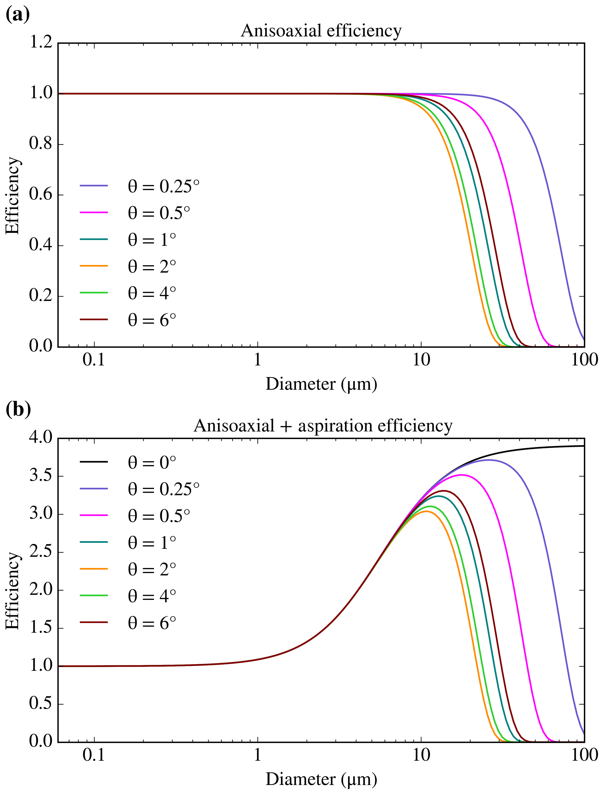
Figure 3 Anisoaxial inertial losses of the sampling carried out by the filter inlet system for different values of the angle in between the inlet and the flight direction. The calculations have been presented by themselves (a) and combined with the aspiration efficiency (b), which one can see in Fig. 2a. The anisoaxial calculations have been carried out using the equations given by Hangal and Willeke (1990b), using the same parameters and dimensions as in Fig. 2, apart from the flow rate, which was set to 65 L min⁻¹ in order to be within the valid range of U∕U₀ that was used to develop the equation. For smaller or larger values of the flow rate (under which most of the sampling is carried out), the differences in the efficiency from the ones shown here are minimal.

One can see all the efficiency mechanisms combined for four different flow rates in Fig. 2b. These have been derived by multiplying all the efficiencies for the individual mechanisms. This overall efficiency is the ratio between the particles that reach the filter and the particles in the ambient air. The sampling efficiency for the submicron aerosol is close to 1. At sizes above 1 µm, the different loss mechanisms become increasingly significant. For the range of flow rates considered, the efficiency approaches zero between 20 and 50 µm, with D50 values in between ∼10 and ∼33 µm (although these values could be lower under certain values of angles of attack if considering the anisoaxial losses from Fig. 3, which have not been included). For the 80 L min⁻¹ case, the flow is turbulent through the whole pipe, leading to enhanced losses of coarse aerosol particles, which partially compensate for the sub-isokinetic enhancement of the system.

One can also see that the sub-isokinetic enhancement of large aerosol particles increases when decreasing the flow rate of the system. This effect is about a factor of 3.5 for 10 µm particles when sampling at 15 L min⁻¹, but only a factor of 2 at 50 L min⁻¹. The sub-isokinetic enhancement can be mitigated using the bypass, which enhances the flow through the nozzle. This can be seen in Fig. 2c where one can see a comparison between the total efficiency of a 20 L min⁻¹ flow rate through the filters with no bypass flow and the same case when the bypass is open. Since the considered bypass flow is comparable to the flow rate through the filters, the difference between the total flows for the two cases is approximately a factor of 2. As a consequence, the maximum sub-isokinetic enhancement of large aerosol particles is almost a factor of 2 larger when sampling with the bypass closed. Hence, the sub-isokinetic enhancement can be reduced by keeping the bypass fully open.

2.3 Sampling flow rate

Here we show flow rate data from four field campaigns in order to examine how the flow rate of the filter inlet system varied based on different factors. We have used the data collected during the ICE-D campaign, in Cabo Verde during August 2015 (Price et al., 2018). The rest of the data are from some flight tests carried out during 2017 and 2018 and three field campaigns. The first one was EMERGE, based in southeast England in July 2017. The second one was VANAHEIM, based in Iceland in October 2017. The last campaign was MACSSIMIZE, based in Alaska in 2018. The flow rate of the inlet system is known to vary with altitude, with a lower flow rate at high altitudes because of the reduced pressure differential across the filter and the fact that the pump efficiency decreases at low pressure. In addition, it changes depending on the filter type and the pore size.

In Fig. 4, where all the flow rate data have been presented, one can see that the flow rate tends to decrease with altitude and change with filter type as expected, but the flow rates are not always consistent for each altitude and filter type, varying up to a factor of 2 for each filter type, line, altitude, and campaign. The filter type effect on flow rate can be seen in Fig. 4, where the average flow rate for 0.4 µm polycarbonate filters is about twice the flow rate of the 0.45 µm PTFE filters. In order to investigate the inconsistency in the flow rate at each altitude, we analysed the flow rate data by comparing them with different parameters (ambient air and cabin temperature, ambient air and cabin pressure, wind direction and speed with respect to the aircraft movement), but there was no correlation with any of these variables. Different mesh supports were used, but this does not affect the flow rate significantly according to some ground-based tests. We checked the flow rate through each sampling period and found it did not change over time on a particular filter set (even after stopping the sampling and starting it again). In addition, we performed some tests on the ground and during flights to study the effect of potential leaks by inserting paper disks of the same dimension as the filters in the filter holders and found no evidence of leaks in the system.

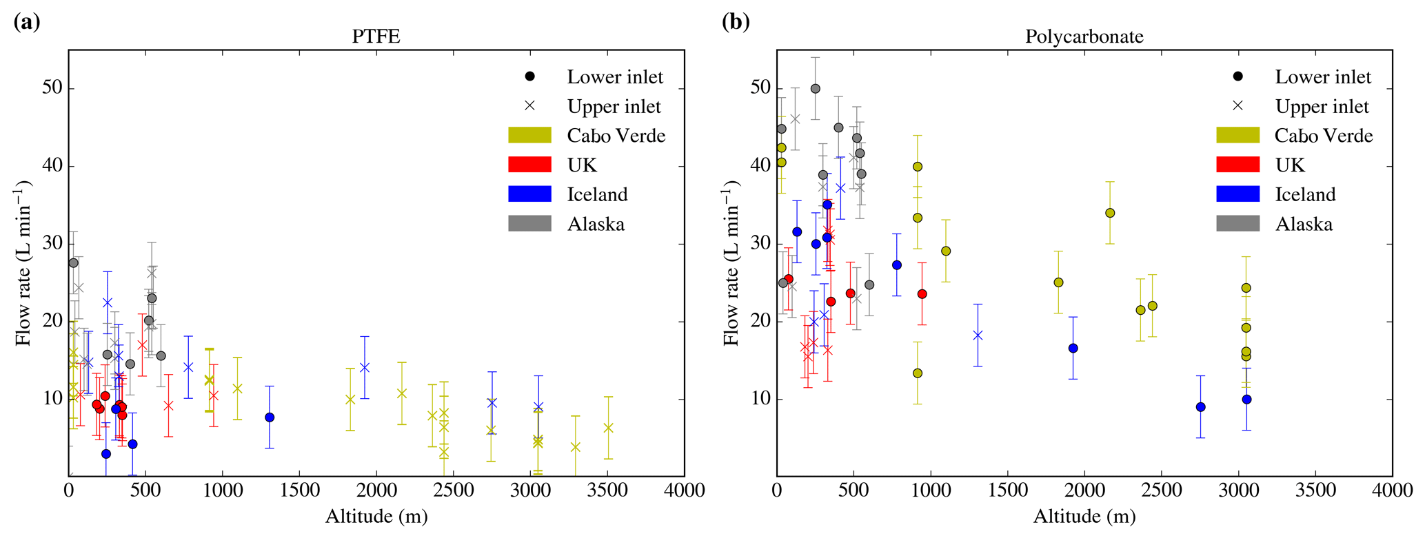
Figure 4 Filter flow rate of different samplings carried out in different campaigns at each altitude using (a) Sartorius PTFE membrane filters (47 mm diameter with a pore size of 0.45 µm) and (b) Whatman nucleopore polycarbonate track etched filters (47 mm diameter with a pore size of 0.4 µm). The crosses represent samples taken in the upper line of the inlet system, whereas dots represent the sampling in the bottom line. Different mesh supports were used for the data collection. The data from Cabo Verde were extracted from Price et al. (2018) and the notes of the analysis carried out by the authors, whereas the altitude data from the other three were obtained from the pressure altitude measurement carried out by the reduced vertical separation minimum system on board the aircraft. The altitude data were extracted from the FAAM core datasets C019, C022, C024, C025, C058, C059, C060, C061, C062, C063, C085, C086, C087, C088, C089, C090, and C091 (via the Centre for Environmental Data Analysis). The bypass was closed for all the data in Cabo Verde whereas it was open for all the data in the other campaigns. Note that the flow rate here corresponds to the filter flow rate (measured with the mass flow meter), not the total one.

We conclude that this variability in the flow rate comes from variability in the pump performance in combination with subtle differences in individual filter pairs. The side displacement pump is not the ideal pump for this system and operates at its maximum capacity. Hence, we suggest that to improve the performance of the system flow rates should be actively controlled and also the side displacement pump should be replaced with a more appropriate design. This would also have the advantage that flow rates would be maintained at smaller pressure drops and allow sampling at higher altitudes.

3 FAAM BAe-146 underwing optical particle counters

Later in the paper we compare results from the underwing optical particle counters with our electron-microscope-derived size distributions; hence we describe the optical instruments here. The FAAM BAe-146 operates underwing optical particle counters to measure aerosol size distributions. These include the passive cavity aerosol spectrometer probe 100-X (PCASP) and the cloud droplet probe (CDP). The PCASP measures particles with diameters in the approximate range 0.1–3 µm and the CDP measures the particles with diameters in the range of 2–50 µm. These instruments are placed outside the aircraft fuselage, below the wings. These instruments and the methods for calibration are described in Rosenberg et al. (2012). All the PCASP–CDP data shown here have been extracted from the FAAM cloud datasets corresponding to each specific flight via the Centre for Environmental Data Analysis.

The instruments were calibrated and had optical property corrections applied as per Rosenberg et al. (2012). We used a refractive index of 1.56+0i and a spherical approximation (Mie theory) in the optical property corrections. In Fig. 5, one can see a sensitivity test on the refractive index value we used in order to examine how variability in refractive index affects the bin centres' position, their width, and therefore the size distribution obtained from the PCASP and CDP. As one can see in Fig. 5a, modification of the real part of the refractive index from 1.5 to 1.7 can change the position of the PCASP bin centres up to a factor of 1.5, but its effect on the CDP is not significant. When varying the imaginary part of the refractive index from 0 to 0.01, the bin centre positions of the first half of the range of the PCASP and CDP do not change but it can change the position of the bins of the end of the range of both instruments (less than a factor of 1.5). However, for the purposes of this work, the differences produced by the variation in the refractive index are not large enough to modify the conclusions of the analysis; therefore we use a value of 1.56+0i.

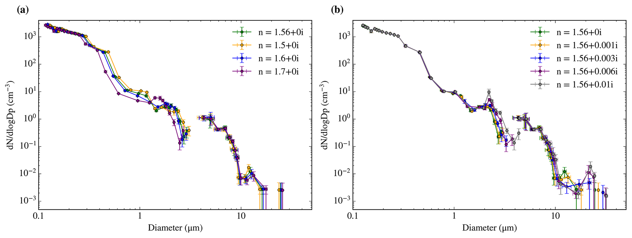
Figure 5 Sensitivity of the size distributions measured by the PCASP–CDP during the C010 flight on 10 May 2017 from 11:24 to 11:38 UTC to small variations in the refractive index. We tested both the real part (a) and imaginary part (b). The errors are calculated according to the methods explained in Sect. 3.

The chosen refractive index range for this sensitivity analysis can be justified on the basis that the SEM compositional analysis showed that the composition of the aerosol samples used in this study was very heterogeneous, dominated by carbonaceous particles (biogenic, organic, and black carbon), and with some contributions of mineral dust and other particle types. Values of the real part of the refractive index in the 1.5 to 1.6 range are compatible with sodium chloride and ammonium sulfate (Seinfeld and Pandis, 2006), as well as most mineral dusts (McConnell et al., 2010). The range is very close to values for the real part of the refractive index of organic carbon but below the values for black carbon (Kim et al., 2015). As a consequence, the refractive index choice might not be accurate for a black-carbon-dominated sample. However, black carbon is highly unlikely to dominate in the size range where a value of the real part of the refractive index of 1.7 dramatically changes the size distribution (diameters above 0.5 µm) (Seinfeld and Pandis, 2006), so our refractive index choice is valid. In Fig. 5b one can see that changing the imaginary part of the refractive index from 0 to 0.01 only produces small changes in the distribution. The imaginary part of the refractive index of many aerosol types such as sodium chloride, sulfates, and mineral dust falls within the shown range (Seinfeld and Pandis, 2006; McConnell et al., 2010). For values of the imaginary part of the refractive index above 0.01 (not shown in the image), the size distribution dramatically changes for sizes above 1 µm (but not for smaller values of it), overlapping and disagreeing with the CDP. However, values above 0.01 in the imaginary part of the refractive index are only associated with strongly absorbing aerosol like black carbon, which will dominate only in the submicron sizes (Seinfeld and Pandis, 2006). The submicron part of the size distribution does not change for values of the imaginary part of the refractive index above 0.01, so our refractive index choice is still acceptable even for samples with significant contributions from black carbon in submicron sizes.

For the PCASP–CDP, we have considered two uncertainty sources. The first one is the Poisson counting uncertainty in the number of particles in each bin and the second one is the uncertainty in the bin width that is given by the applied optical property corrections. Both sources have been propagated in order to obtain the errors of dN ∕ dlogDp and dA ∕ dlogDp. The errors in the bin centre position were given by the calibration. In order to avoid the problems with the transition in between different gain stages in the PCASP, some bins were merged or eliminated (5 and 6 as well as 15 and 16 were merged, while bin 30 was eliminated), as indicated by Rosenberg et al. (2012). Other uncertainties such as the refractive index assumption or particle shape effect, as well as the uncertainty in the bin position have not been regarded in this study. Sampling biases have not been quantified or corrected yet, so they have not been included. The size distributions produced by the PCASP–CDP have been taken as a reference value for the purposes of this study.

4 Scanning electron microscopy technique for aerosol characterisation

Scanning electron microscopy is used in order to study composition and morphology of aerosol particles, in a similar way to previous works such as Krejci et al. (2005), Kandler et al. (2007), Chou et al. (2008), Kandler et al. (2011), Young et al. (2016), Price et al. (2018), and Ryder et al. (2018). We use a Tescan VEGA3 XM scanning electron microscope (SEM) fitted with an X-max 150 SDD energy-dispersive X-ray spectroscopy (EDS) system controlled by an Aztec 3.3 software by Oxford Instruments, at the Leeds Electron Microscopy and Spectroscopy Centre (LEMAS) at the University of Leeds. In order to obtain data from thousands of particles in an efficient way, data collection was controlled by the AZtecFeature software expansion.

Aerosol particles were collected with the filter inlet of the FAAM BAe-146 on polycarbonate track etched filters with 0.4 µm pores (Whatman, Nucleopore). Samples for SEM are usually coated with conductive materials in order to prevent the accumulation of charging on the sample surface (Egerton, 2005). For aerosol studies, materials like gold (Hand et al., 2010), platinum (Chou et al., 2008), or evaporated carbon (Krejci et al., 2005; Reid et al., 2003; Young et al., 2016) have been used. When it comes to choosing which signal to detect, some previous studies used mainly backscattered electrons (Gao et al., 2007; Kandler et al., 2007, 2011, 2018; Price et al., 2018; Reid et al., 2003; Young et al., 2016) and some others choose secondary electrons (Hamacher-Barth et al., 2013; Krejci et al., 2005). We started the development of this analysis using a carbon coating and the backscattered electron detector. This technique produced reproducible images and almost no artefacts from the pore edges, consistent with Gao et al. (2007). However, we noticed that we sometimes undercounted a significant fraction of the small carbon-based particles (this strongly depended on the sample), which looked transparent under the backscattered electron imaging but not under the secondary electron detector, as seen in Fig. 6. This likely happened because the contrast in the secondary electron images mainly depends on the topography of the sample, whereas the contrast in the backscattered electron images depends on the mean atomic number of each sample phase (Egerton, 2005). Since the polycarbonate filters are made of C and O, particles containing only these elements in a similar proportion to the background did not exhibit a high contrast under the backscattered electron detector (Laskin and Cowin, 2001). However, when using secondary electron imaging with carbon coatings, images were less reproducible and contained artefacts from the pore edges, probably resulting from charging or topographical effects. We found that coating the samples with 30 nm of iridium helps to improve the secondary electron image reproducibility and reduced the pore edge artefacts as well as allowing us to locate small organic particles. An increase in the size of the particle as a consequence of the coating may introduce an uncertainty in the size of the smallest particles. An additional advantage of using Ir is that the energy-dispersive X-ray spectrum of Ir does not overlap greatly with the elements of interest.

Figure 6 Secondary electron image (a) and backscattered electron image (b) of the same area of the same filter, collected in SE England on 5 July 2018 from 13:32 to 13:47 UTC in the upper line with the bypass open. As one can see, some of the small particles in the secondary electron image appear almost transparent under the backscattered electron image. Even the 10 µm soot particle in the bottom left of the image shows a very low contrast in the backscattered electron image.

In the SEM the sample was positioned at a working distance of 15 mm. The SEM's electron beam had an accelerating voltage of 20 KeV and a spot size chosen to produce the optimum number of input counts in the EDS detector. Images are taken at two different magnifications with a pixel dwell time of 10 µs and a resolution of 1024×960 pixels per image. High-magnification images (40 nm per pixel or smaller) were used to identify particles down to 0.3 or 0.2 µm depending on the sample, and medium-magnification images (about 140 nm per pixel) are used to identify particles down to 1 µm. A brightness threshold with upper and lower limits that correspond to pixels of certain shades of grey was manually adjusted for each image by the operator to discriminate particles from the background. Based on the manually set brightness threshold, AZtecFeature identified the pixels that fall within the limits as aerosol particles and calculated several morphological properties of the particle as cross-sectional area, length, perimeter, aspect ratio, shape factor, or equivalent circular diameter. The equivalent circular diameter is defined as $\surd \left(\mathrm{4}A{\mathit{\pi }}^{-\mathrm{1}}\right)$, where A is the cross-sectional area of the aerosol particle. This equivalent circular diameter has not been corrected or transformed into an optical or other equivalent diameter.

For this analysis we placed a section of the 47 mm filter on a 25 mm stub. In order to collect morphological and chemical information from a few thousand particles, we only scanned a fraction of the filter (typically up to 1 % of the filter at low magnification and up to 0.01 % for high magnification). We collected information from 5 to 20 different areas, and each area consisted of a montage of several SEM images. In Fig. 7 one can see the radial distribution of aerosol particles on top of a filter collected using the inlet system. In spite of some fluctuations (which are up to a factor of 3 and appear to be random), one can see that the particles are homogenously distributed all over the central ∼30 mm of the filter. As a consequence, the areas were chosen by the user from all over the surface of the selected fraction of the filter. Each area was selected in the software, manually adjusting the particle detection threshold. The Z position of the stage was also adjusted manually for each image in order to produce properly focused images. After doing this, the image scanning and EDS acquisition was performed in an automated way. Morphological information was recorded for all particles with an equivalent circular diameter greater than the specified size threshold (typically 0.2 or 0.3 µm).

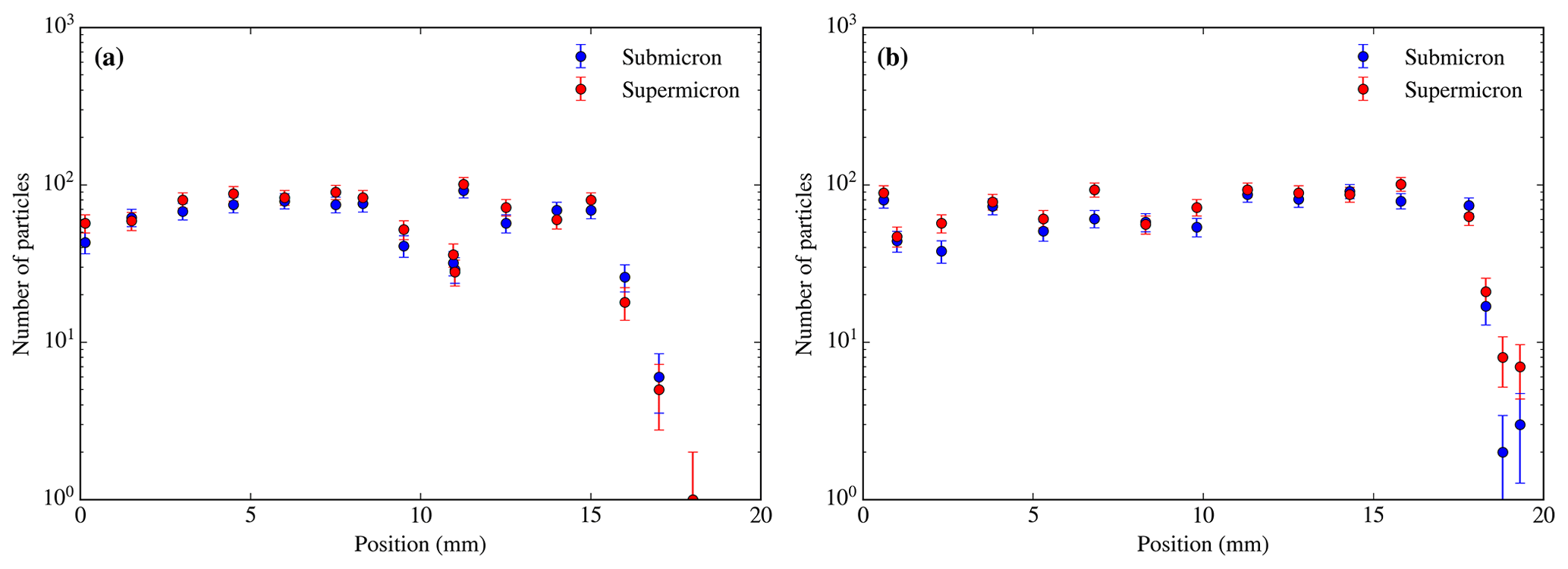
Figure 7 Radial distribution of the particle test on the sample collected on 2 October 2017 (flight C059) from 16:24 to 16:40 UTC at about 320 m in altitude in southern Iceland, using the lower line and open bypass, sampling 432 L. Number of submicron and supermicron particles in same size areas ($\sim \mathrm{160}\times \mathrm{190}$ µm²) radially distributed versus the distance from the approximate centre through a radius of the filter (a) and another trajectory from the centre of the filter deviated 30^∘ from the first radius (b). The analysis was performed at 20 KeV and ×5000. The number of both supermicron and submicron particles remains very constant all over the surface of the filter, until reaching the edges of it (which are cover by a rubber O-ring during the sampling) and the number of particles drops to the limit of the detection within a few millimetres. The error in the number of particles comes from Poisson counting statistics.

EDS analysis was restricted to the first 12 or 15 particles detected in each image. This reduces the likelihood of image defocusing over the SEM automated run. The software performed EDS in the centre of the particles, obtaining around 50 000 counts per particle. The raw data for any given particle were matrix corrected and normalised by the AZtec software to produce element weight percent values with a sum total of 100 %, using a value of the confidence interval of 2 (a further discussion on the confidence interval can be seen in the Appendix C). Then particles were categorised based on their chemical composition using a classification scheme which can be created and modified within the AZtecFeature software. The characteristic X-rays taken at one point are emitted by a certain interaction volume which is bigger than some of the analysed particles (typically < 2 µm³, decreasing with atomic number and increasing with incident electron energy). As a consequence, a part of the X-ray counts attributed to each particle come from the background (C and O from the polycarbonate filter and Ir from the coating) and the weight percentages obtained from the X-ray spectra do not match the actual weight percentages of the particle itself. As a consequence, when categorising the particles based on their composition, we only use the presence or absence of certain elements, and the ratio between the weight percentages of non-background elements. The classification scheme works by checking if the composition of each particle falls within a range of values which are manually defined by the user. Particles not matching the first set of rules are tested again for a second set of rules, and so on, until reaching the last set of rules. A few sets of rules can be merged into a category. In the Supplement (Fig. S3), we give the details of the 32 sets of rules used, which are then summarised into 10 composition categories. A description of the most abundant elements in each category and an interpretation of these categories are included in Appendix B.

The detection of particles has certain limitations. The edges of the pores can look brighter than the rest of the filter in the SE images (probably because they consist of a larger surface area from which secondary electrons can be generated, hence a larger signal). As a consequence, they can look like ∼0.2 µm particles, which is the main reason why particles below 0.3–0.2 µm (depending on the sample) are not included in this analysis. These artefacts had a chemical composition similar to the filter, so they were labelled as “carbonaceous” by the classification scheme, falling at the same category as most biogenic and black carbon particles. However, these artefacts were only around 1 % to 10 % depending on the sample. If they appear in larger quantities, they can be removed manually after or during the analysis. Another limitation arises from the fact that some aerosol particles did not have sufficient brightness in the SE image and were not detected as a particle. This happens more frequently for submicron particles (especially the ones closer to the limit of detection), but it can also happen with some coarse-mode aerosol particles, particularly if they are only composed of Na and Cl or S. This issue can be addressed if necessary by setting a very low limit of detection, which adds lots of artefacts as well as the low brightness particles, and then removing the artefacts manually (the artefacts can be easily identified by the user). In other infrequent instances, only a fraction of the particle had a brightness above the threshold, so they were detected as a smaller particle or multiple smaller particles, or if two particles are close enough, they can be detected as a single larger particle. However, we feel that in the vast majority of the cases a representative cross-sectional area of the particle was picked by the software.

Blank polycarbonate filters can contain some particles on them from manufacturing or transport before being exposed to the air. In addition, handling and preparing the filters can introduce additional particles to it. In order to assess these artefacts, we scanned a few clean blank filters. We also examined a filter that had been brought to the flight, loaded in the inlet system (but not exposed to a flow of air), and then stored at −18 ^∘C for a few months (like most of the aerosol samples on filters). The results of both the handling blank and the blank can be seen in Fig. S2. The number of particles is typically about the order of magnitude of one particle per 100 µm by 100 µm square, which is more than an order of magnitude below all the samples in this study (apart from the sample shown in Fig. 9c, which was taken in a very low aerosol environment, where it is only about a factor of 2). In Fig. S2 one can see that about half of particles found in both blank filters and the handling blank belong to the metal-rich category. However, further examination of the composition of these metal-rich particles revealed that almost all of them were Cr-rich particles (about 97 % in the case of the blank filters and about 96 % in the case of the handling blank). As a consequence, we excluded all the Cr-rich particles from the analysis of atmospheric aerosol. By doing this, we make sure that we exclude about half of the artefacts of the analysis. There was a contribution of mineral dust origin particles (Al–Si rich, SI rich, and Si only) for sizes in between 0.7 and 5 µm in the handling blank (less than 10 % of the number in the handling blanks). Generally, the composition of the particles present in the blank filters and in the handling blank was very similar, suggesting that most of these artefacts are not produced by the loading, manipulation, and storage of the filter.

5 Inlet characterisation and sampling efficiency using scanning electron microscopy

In order to experimentally test the inlet efficiency, to complement the efficiency calculations presented in Sect. 2.2, we have used SEM to quantify the size distribution of particles collected on filters (Sect. 4) and compare this with the measurements from the underwing optical probes (Sect. 3). The calculations in Sect. 2.2 suggest that there is an enhancement of the coarse-mode aerosol particles, which is larger when sampling with the bypass closed. To test this we have collected aerosol onto a 0.4 µm pore size polycarbonate filter in both lines in parallel and show these results in Fig. 8. In one of the lines, the bypass was kept open, and in the other line the bypass was kept closed. Using our SEM approach described in the Sect. 4, we calculated the size distribution of the aerosol particles on top of each filter. We compared these size distributions with the ones measured by the underwing optical probes (PCASP–CDP), as described in Sect. 3. We performed the comparison twice in two different test flights based in the UK.

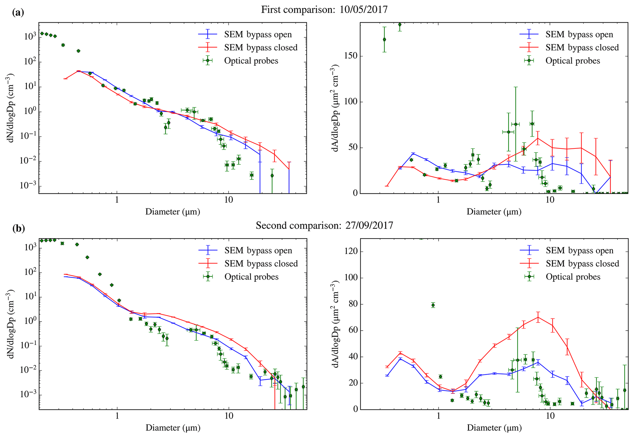
Figure 8 (a) First bypass test carried out during the C010 flight on 10 May 2017 from 11:24 to 11:38 UTC. The lower line sampled 226 L with the bypass closed, whereas the upper line sampled 141 L with the bypass open at an altitude of about 150 m. The flow rates were 16.1 and 10.6 L min⁻¹ respectively. (b) Second bypass test carried out during the C057 flight on 27 September 2017 from 13:33 to 13:50 UTC. The lower line sampled 555 L with the bypass open, whereas the upper line sampled 499 L with the bypass closed, at about 240 m. The flow rates were 34.7 and 31.2 L min⁻¹ respectively. The position of the closed and open lines was swapped with respect to the first comparison. The sampling was interrupted for a minute to avoid a turn. Both comparisons are shown in both number size distribution and surface area size distribution. The optical probes are the PCASP–CDP, using the closest calibration to the sampling date and a refractive index of 1.56 as stated in Sect. 2.3. The only error source considered for the SEM size distribution is the Poisson counting error.

One can see that the concentration of aerosol particles measured by the SEM on the filters was higher than the particles detected by the optical probes for sizes above ∼8 µm in Fig. 8 (reaching about an order of magnitude in number around 10 µm in both cases). These results are consistent with Price et al. (2018) and Ryder et al. (2018), where they observed an enhancement of coarse aerosol particles in mineral-dust-dominated samples collected close to Cabo Verde. In addition, the enhancement was larger when sampling with the bypass closed (about a factor of 2–3). The results of these comparisons are in qualitative agreement with the theoretical calculations in Sect. 2.2, i.e. that the sub-isokinetic enhancement is reduced with the bypass open.

After establishing that having the bypass open produces a more representative sampling of coarse-mode aerosol, we then had the open-bypass for the subsequent sampling. In Fig. 9 we have presented some other bypass open SEM size distributions compared with the PCASP–CDP data from three different aerosol samples in contrasting locations. Since these data were taken during the scientific field campaigns and not test flights, we only collected one polycarbonate filter for SEM since the other line was used for INP analysis on Teflon filters (not shown here). In Fig. 9a, one can see a sample collected in the UK where there is an enhancement of the coarse mode which reaches almost an order of magnitude at 10 µm. The sample shown in Fig. 9b was collected in Iceland, and the enhancement of coarse aerosols can be seen through most of its range, reaching even the first two bins of the submicron aerosol range. In Fig. 9c one can see a sample collected in northern Alaska where the coarse-mode aerosol concentration was 1 to 2 orders lower than the examples from the UK and Iceland. In this case the SEM size distribution is only about a factor of 2 above the size distribution of the handling blank; nevertheless the SEM and optical probes both produce similarly low numbers of coarse-mode aerosol. The low number concentration results in the lack of data in the SEM above 7 µm and the large uncertainties in the PCASP–CDP above 1.5 µm. We do not observe a coarse-mode enhancement in this sample, probably because of the low aerosol concentration in the size range where we expect the largest biases and large uncertainties.

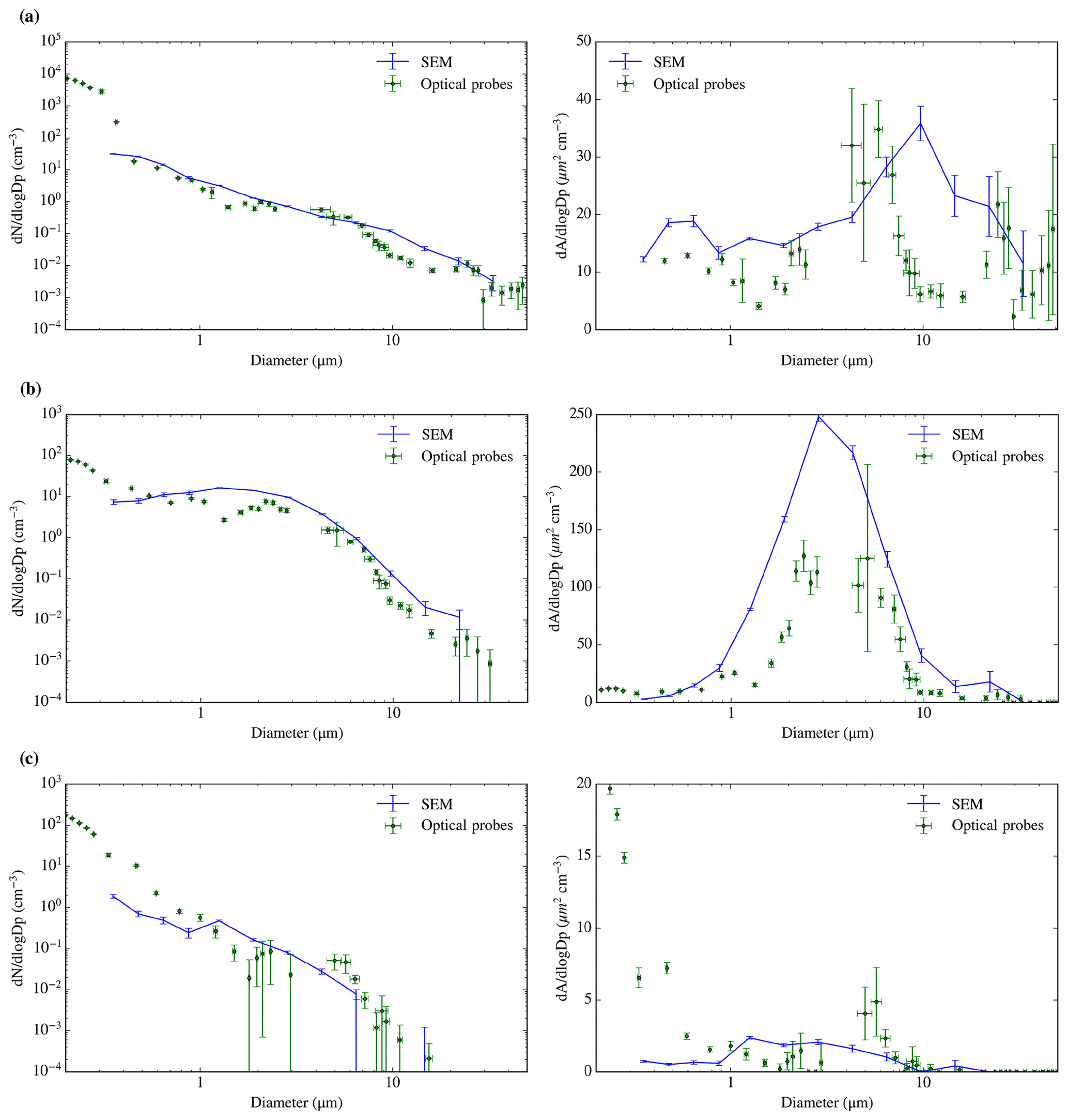
Figure 9 SEM-obtained size distribution compared with PCASP–CDP online size distribution for three different sampling periods in three different aerosol environments. Close to London, on 19 July 2017 (flight C024) from 15:20 to 15:51 UTC, sampling 953 L (a); south of Iceland on 2 October 2017 (flight C059) from 16:24 to 16:40 UTC, sampling 432 L at an altitude of about 320 m (b); and in northern Alaska on 20 March 2018 (flight C090) from 20:15 to 20:37 UTC, sampling 724 L (c). All the sampling was performed in the upper line with the bypass open. The flow rates through the filter holders are 30.9, 30.5, and 42.0 L min⁻¹ respectively. The optical probes are the PCASP–CDP, using the closest calibration to the sampling date and a refractive index of 1.56 as stated in Sect. 2.3.

In the submicron range, one can see that in all the comparisons shown in Figs. 8 and 9 there is sometimes an undercount in the SEM size distribution when compared with the optical probes. Generally, the undercount increases with decreasing size and reaches an order of magnitude or more, as one can see in Figs. 8, 9a, and c; this is qualitatively similar to Young et al. (2016). There are several potential reasons for this. We can rule out particles simply being lost by passing through the 0.4 µm polycarbonate filters since they are known to have a high collection efficiency (Lindsley, 2016; Soo et al., 2016), although some of them might deposit inside the pores and therefore not be detected. In addition, it is likely that some small particles are not sufficiently bright to be detected, despite the fact we made efforts to mitigate this problem with the use of secondary electrons and the Ir coating (see Fig. 6). Also, volatilisation of certain types of aerosol particles (which are more abundant in the submicron fraction; Seinfeld and Pandis, 2006) can occur during heating (in this case produced by deceleration of the flow in the inlet) or sampling (Bergin et al., 1997; Hyuk Kim, 2015; Nessler et al., 2003) and this effect could be enhanced by the fact that samples are exposed to high vacuum during the SEM analysis. In addition, the SEM techniques measure the dry diameter and the optical probes measure the aerosol diameter at ambient humidity. This hygroscopic effect shifts the dry size distributions to smaller sizes, which might also explain part of the disagreement (Nessler et al., 2003; Young et al., 2016). Disagreement in the measurements can also be produced by the fact that the techniques are measuring different diameters (optical and geometric).

Some of the PCASP size distributions contain some “bumps” (particularly above 2 µm), but it is not possible to address if they are physical or just an artefact produced by the refractive index correction (Rosenberg et al., 2012). Given the uncertainties on both techniques and the fact that they measure different diameters (optical diameter in the case of the PCASP–CDP and geometric equivalent circular diameter in the case of the SEM), this comparison cannot be used to quantify the biases in the system, but can be used to make a qualitative comparison. For similar reasons, the SEM data have not been corrected using the theoretical efficiency.

6 Application to samples collected from the atmosphere above SE England and northern Alaska

The SEM technique to produce size-resolved composition of aerosol samples described in Sect. 4 has been applied to samples collected from the FAAM BAe-146 in various locations. In Fig. 10 we show an example of some of the capabilities of this technique applied to a sample collected in SE England. The purpose of this section is purely to give examples of the capabilities of the technique; further analysis is planned for subsequent papers. The fraction of particles corresponding to each compositional category described in Appendix B for each size can be seen in Fig. 10a and the corresponding number size distribution of each composition category can be seen in Fig. 10b. By looking at this analysis, one can see that the sample carbonaceous aerosol particles made a substantial contribution to the number across the full distribution and there was a clear mineral dust mode (Si only, Si rich, Al–Si rich, and Ca rich) for particles larger than about 1 µm. There was also a smaller contribution of metal-rich and S-rich aerosol particles, particularly in the fine mode. A potentially useful application of the size-resolved composition is calculating the surface area or mass of an individual component of a heterogeneous aerosol. As an example, we have grouped the mineral dust categories Si only, Si rich, Al–Si rich, and Ca rich to produce the surface area size distribution of mineral dust (and potentially ash) in Fig. 10c.

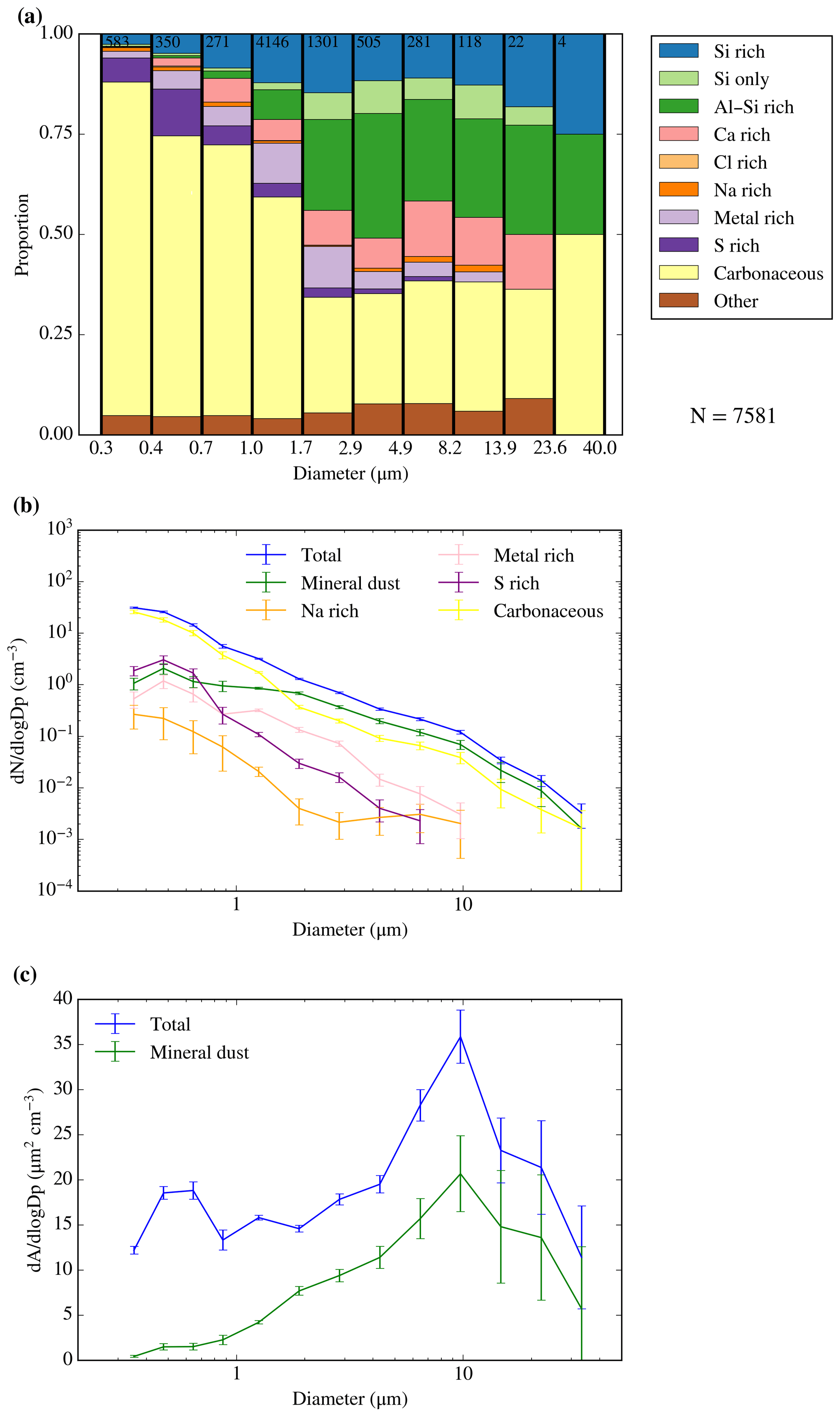
Figure 10 Size-segregated compositional and morphological analysis of a sample collected close to London (SE England) on 19 July 2017 from 15:20 to 15:52 UTC by the lower line with the bypass open, sampling a total of 953 L at 350 m altitude. (a) Fraction of particles corresponding to each compositional category (described in the Appendix B) for each size. The number of particles per bin can be seen in the top of the figure. (b) Number size distribution for each composition. Cl-rich particles were not included since only two particles in this category were found. The errors have been calculated from the Poisson counting statistics (applying it to both the size distribution and the compositional measurements). (c) Surface area of both all the detected aerosol particles and the ones whose composition was consistent with mineral dust. Errors have been calculated in the same way as before. By integrating the green curve in (c) we obtained the total surface area of mineral dust in the sample (19.1 µm² cm⁻³).

In Fig. 11 we show six examples of the size-resolved composition of different aerosol samples in two locations (southeast England and northern Alaska). We can see that the aerosol samples are very different depending on the location. The aerosol samples collected in the UK shown in Fig. 11a, c, and d are very similar to the sample shown in Fig. 10a. In fact the sample in Fig. 10a was taken on the same day in a similar location as the sample in Fig. 11b and the similarity between the two helps to demonstrate the reproducibility of our technique. Generally, these samples from SE England contained carbonaceous aerosol throughout the size distribution, particularly in the fine mode. This is consistent with typical urban aerosol (Seinfeld and Pandis, 2006). There is also a substantial proportion of mineral dust and only a small proportion of Na-rich aerosol. In contrast, the samples collected in northern Alaska (close to or above the Arctic Ocean) generally contained a smaller proportion of carbonaceous particles, but much larger contributions of Na-rich aerosol (very likely sea salt particles, since they were collected in a marine environment). The S-rich category was also substantial in the fine mode in Alaska, consistent with some samples collected in other areas of the Arctic (Young et al., 2016) and some samples collected in a similar location (Creamean et al., 2018). Notably, the coarse mode in Alaska, while generally smaller in number than in SE England, contained a high proportion of mineral dust. This is also consistent with other measurements in the Arctic (Creamean et al., 2018; Young et al., 2016).

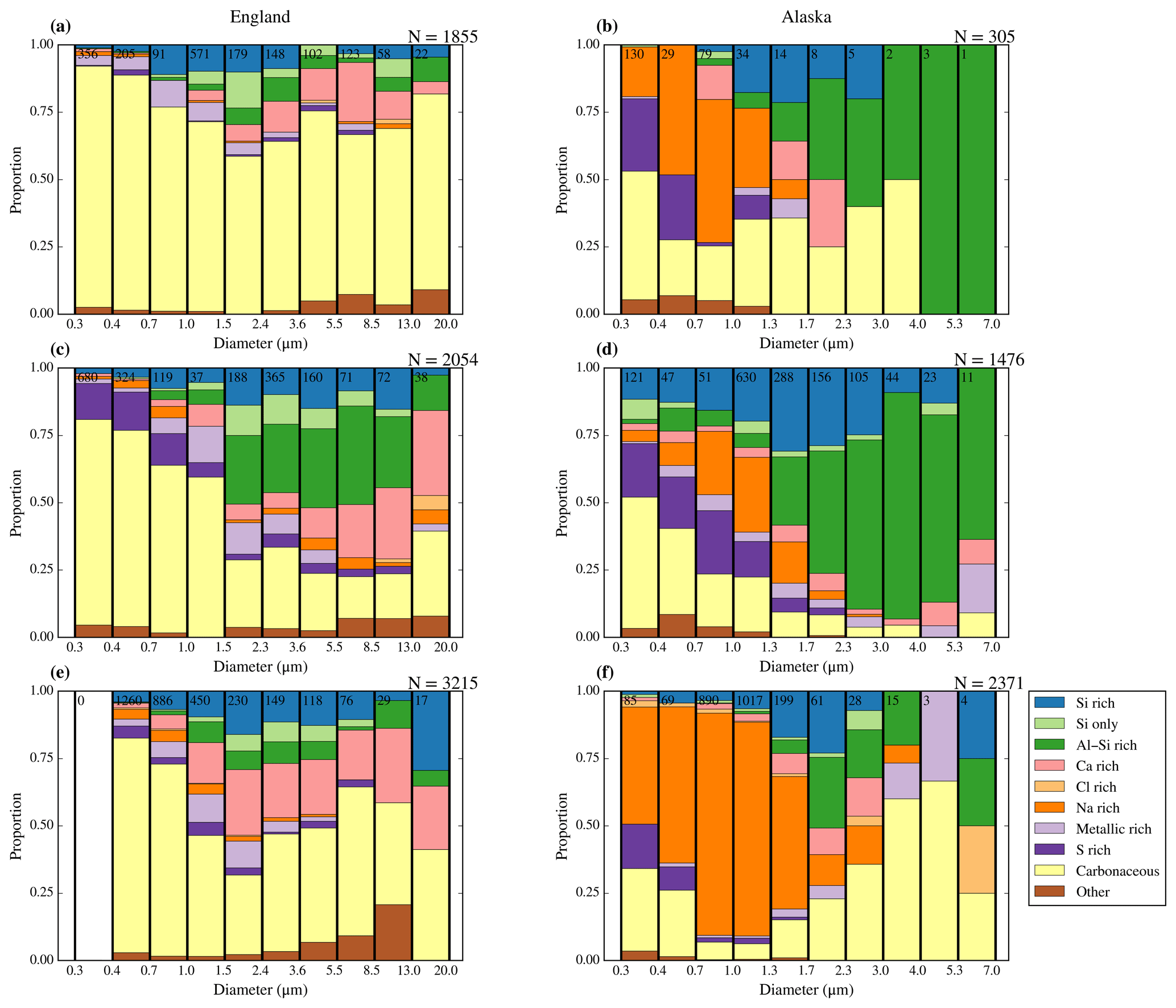
Figure 11 Six examples of the size-resolved composition of aerosol sampled from the BAe-146 aircraft above south England (a, c, e) and northern Alaska (b, d, f). All the samples were taken with the bypass open. The dates and sampling times (UTC) are (a) 17 July 2017 (flight C022) from 09:29 to 09:41, sampling a total of 182 L at an altitude of about 240 m; (b) 18 March 2018 (flight C089) from 19:28 to 19:48, sampling a total of 404 L at an altitude of about 600 m; (c) 19 July 2017 (flight C024) from 15:20 to 15:52, sampling a total of 256 L at an altitude of about 350 m (this sample was taken on the same day as the one shown in Fig. 10); (d) 20 March 2018 (flight C090) from 20:15 to 20:37, sampling a total of 724 L at an altitude of about 520 m; (e) 20 July 2017 (flight C025) from 12:51 to 13:09, sampling a total of 425 L; and (f) 21 March 2018 (flight C091) from 18:27 to 18:56, sampling a total of 1187 L at an altitude of about 120 m at an altitude of about 940 m.

7 Recommendations for aerosol sampling with the filter system on the FAAM BAe-146

Based on the calculations in Sect. 2.1 and the experimental findings in the subsequent sections, we suggest keeping the total flow rate (including the flow through the filters measured by the electronics box plus the bypass flow, which can be between 20 and 35 L min⁻¹) above 50 L min⁻¹. Below this range, the sub-isokinetic enhancement of large aerosol particles is above a factor of 2, according to the calculations in Sect. 2.2 that can be seen in Fig. 2b. For total flow rates above 65 L min⁻¹, the flow becomes turbulent throughout the line, which is associated with losses. However, the calculations shown in Fig. 2c indicate that the combination of the isokinetic enhancements and turbulent losses at 80 L min⁻¹ lead to a reasonably representative sampling, but when it reaches 150 L min⁻¹, the position of the D50 drops to 6.5 µm (not shown in the graph) so such a high flow rate would not be appropriate if the user wants to sample coarse aerosol particles. Hence, we recommend an operational upper limit of 80 L min⁻¹. For 0.45 µm PTFE filters and the 0.4 µm polycarbonate filters presented in Fig. 4, sampling close to this flow rate range is often achievable by keeping the bypass open since this increases the total flow rate and brings it closer to the suggested range, as one can see in Fig. 2c. If other filter types are used, the flow rates will be different to those presented here and these flow rates should be taken into consideration when choosing the pore size (or equivalent pore size) in order to avoid dramatic sampling biases.

We already mentioned in Sect. 2.3 that we recommend replacing the side displacement pump with a design that would provide a greater pressure drop. In addition, we also recommend that the bypass flow rate is also routinely measured and controlled in order for the flow at the inlet nozzle to be optimised while sampling.

8 Conclusions

In this work we have characterised the filter inlet system on board the FAAM BAe-146-301 Atmospheric Research Aircraft, which is used for the collection of atmospheric aerosol particles for offline analysis. Our primary goal is to use this inlet system for quantification of INP concentrations and size-resolved composition measurements, but it could also be used to derive other quantities with other analytical techniques.

In order to characterise the inlet system we made use of an electron microscope technique to study the inlet efficiency, by comparing the SEM size distributions with the in situ size distributions measured with underwing optical probes (PCASP–CDP). In spite of the discrepancies and uncertainties, the sub-isokinetic enhancement of large aerosol particles predicted by the calculations in Sect. 2.2 was observed in these comparisons. We also experimentally verify that this enhancement is minimised by operating the inlet with the bypass open, which maximised the flow rate through the inlet nozzle. In addition, we note that we performed tests with three very different aerosol distributions and the size distribution of the particles on the filters had features and concentrations comparable to those measured by the underwing optical probes. Overall, the inlet tends to enhance the concentration of aerosol in the coarse mode with a peak enhancement at ∼10 µm, but when operated with the recommended flow conditions this enhancement is minimised. The inlet efficiency decreases rapidly for sizes above about 20 µm and becomes highly dependent upon the specifics of the sampling such as flow rates and angle of attack. Based on the calculations we recommend that the total flow rates at the nozzle are maintained at between 50 and 80 L min⁻¹, and also that improvements are made to the pump and bypass flow control (see Sect. 2.3).

We also established an SEM technique to determine the size-resolved composition of the aerosol sample. Each particle can be categorised based on its chemical composition using a custom-made classification scheme. Using this technique we showed that the filter system on board the FAAM BAe-146 spreads the particles evenly across the filter surface, which is necessary for the SEM size distribution analysis.

Having a well-characterised inlet allows us to sample aerosol particles up to around 20 µm with knowledge of the likely biases from the aircraft. Hence, we can use this inlet system to collect aerosol for offline analysis at altitudes which are relevant for clouds. For example, this may allow us to use the size-resolved aerosol composition to quantify the size distribution of individual aerosol components at a particular location and combine this information with INP measurements to quantify the surface-area-normalised ice-nucleating ability of a specific class of aerosol.

Appendix A: Discussion of the inlet efficiency calculations

Here we include a further description of the efficiency mechanisms used in the inlet model described in Fig. 2 and discuss the choice of the equations and their limits of validity.

Aspiration efficiency accounts for the fact that the speed of the sampled air mass (U₀) and the speed of the air through the beginning of the nozzle (U) are different. When these two speeds are equal, the sampling is called “isokinetic”, whereas when the speeds do not match, the sampling is called super-isokinetic or sub-isokinetic depending on if U₀ is smaller or larger than U respectively. In our case, the air mass moves at the flying speed, which varies with the altitude (110 m s⁻¹ is a typical value for sampling altitudes), and the speed at the start of the inlet is almost always below 35 m s⁻¹ (sub-isokinetic conditions). As a consequence, some air streamlines will be forced around the inlet, while high-inertia particles will not, which will lead to an aspiration efficiency above 1 for coarse-mode aerosol particles. This enhancement is greater for large particles due to their large inertia, which makes it difficult to follow the air streamlines. The enhancement reaches a maximum value of U₀∕U in its high diameter limit (when none of the particles in the sampled air mass follow the streamlines that escape from the inlet and all of them are sampled). The aspiration efficiency tends to 1 (no enhancement) for small diameters.

This behaviour has been characterised by several studies (we will only look at the sub-isokinetic range of the equations since it is impossible to reach the super-isokinetic range during flight). An empirical equation was developed based on laboratory experiment by Belyaev and Levin (1972) and Belyaev and Levin (1974) (referred to as B&L) for certain ranges of U∕U₀ ratio and Stokes number. However, for ratios below its experimental range (U∕U₀ > 0.2), the B&L function does not make physical sense since it converges to values above 1 for small particle sizes. The aircraft inlet system works at smaller U∕U₀ ratios sometimes, so this function is not very accurate to describe the behaviour of the system in such conditions. Liu et al. (1989) developed another function (referred to as LZK) by means of a numerical simulation based on computational fluid mechanics. The valid U∕U₀ ratio and Stokes number range is wider than the B&L expression (down to 0.1). It agrees with the B&L expression in the U∕U₀ ratio the latter was developed for. For smaller values of the ratio, the LZK function is believed to be more accurate since it predicts the known physical behaviour (no sub-isokinetic enhancement for small particle sizes). It reaches U∕U₀ ratios down to 0.2, which is enough to cover most of the total flow rates achieved in the inlet system. Krämer and Afchine (2004) developed another expression (referred to as K&A) for 0.007 < U∕U₀ < 0.2 based on computational fluid dynamics. However, for low particle sizes, the efficiency does not converge to 1. As a consequence, we have used the LZK (Liu et al., 1989) function since it covers most of the U∕U₀ ratios we get in the inlet system, it agrees with the experimental data in Belyaev and Levin (1972) and Belyaev and Levin (1974), and it converges to U₀∕U for large particle sizes and 1 for small particle sizes. Outside its valid range (U∕U₀ < 0.1), the LZK function agrees with the K&A function for a large radius and converges to 1 for small particle sizes. The equation is valid for 0.01 < Stks < 100, which is enough to cover the range in between 1 and 100 µm. As already stated, it tends to 1 for small particle sizes and to U₀∕U for large particle sizes (at 50 L min⁻¹, the ratio U∕U₀ is 0.2). All the calculations were performed under standard conditions (0 ^∘C and 1 bar). The effect of changes in pressure and temperature (and therefore air density and dynamic viscosity) that normally occur in the filter inlet system sampling range (0 to 3000 m) is negligible in all the used equations as shown in Fig. S1.

The used equations (as well as the ones used for anisoaxial losses) have been developed for thin-walled nozzles (this criterion was defined first in Belyaev and Levin, 1974). The inlet has been described as thin-walled in the literature (Andreae et al., 2000; Formenti et al., 2003; Talbot et al., 1990) but we have not used this terminology here since it is not possible to numerically quantify this using the criteria given in Belyaev and Levin (1974) because the edge of the nozzle is curved. However, the inlet has been designed to avoid distortion of the pressure field at the nozzle tip and the resulting problems associated with flow separation and turbulence (Andreae et al., 1988), which is the main caveat of inlet nozzles that are not thin-walled (Belyaev and Levin, 1974). As a consequence, we used these sets of equations for thin-walled nozzles to describe the filter inlet system considered in this study. The fact that the calculations performed using these equations show that the filter inlet system has biases with similar characteristics as the ones estimated experimentally for coarse aerosol particles helps to support this assumption.

Inlet inertial deposition is defined as the inertial loss of aerosol particles when they enter the nozzle. It is produced by the fact that the streamlines bend towards the walls at the moment they enter the nozzle, and some high-inertia particles can impact the walls and get deposited. Here, we have used the equation given in Liu et al. (1989), which quantifies this effect. It is also valid for 0.01 < Stks < 100, which is enough to cover the range in between 1 and 100 µm.

Turbulent inertial deposition happens when some particles are collected by the wall when travelling in a pipe in the turbulent regime because some of the particles cannot follow the eddies of the turbulent flow. In order to include this mechanism, we used the equation given in Brockmann (2011), using the relation in between the deposition velocity and dimensionless particle relaxation time given by Liu and Ilori (1974). These calculations are valid for a cylindrical pipe, whereas the turbulent section of the inlet considered here is the nozzle, which has a conical shape. In order to account for this, we divided the conical nozzle into 90 conical sections with an increasing diameter and a length of 1 mm, and we combined the effect of all the sections. This approach does not account for the additional inertial losses that could occur as a consequence of turbulence created by the enlargement of the flow in the conical section. However, the angle of enlargement is small (5.7^∘). It was designed to be below 7^∘ in order to avoid flow separation (Andreae et al., 1988). As already mentioned, above 65 L min⁻¹, turbulent flow occurs in the whole inlet tube. This has been taken into account in the 80 L min⁻¹ case in Fig. 2b. The equation used here has been tested for size ranges in between 1.4 and 20 µm, and does not depend on the Reynolds number values it was tested for (10 000 and 50 000) (Liu and Ilori, 1974).

Bending inertial deposition was also considered since the line curves with an angle of 45^∘ in order to bring the airstream into the cabin. The inertia of some particles may keep them in their original track and they are not able to follow the air streamlines that are bending towards the cabin, following the inlet tubes. In order to account for these losses, we have used the empirical equation given in Brockmann (2011) based on the data from Pui et al. (1987) for laminar flow. This equation was developed for Reynolds numbers of 1000, and we have used it for higher values. However, in Brockmann (2011), one can see that the data from Pui et al. (1987) for Re =6000 (beginning of the turbulent flow regime) do not differ that much from the fit we have used (valid for Re =1000). Since our Re numbers for the thick section of the tube almost never go above 5000, we can still use the laminar flow fit. This model has been tested for 0.08 < Stks < 1.2, which is enough to cover most of the range where the inertial deposition efficiency drops from 1 to 0. The main caveat of this calculation is that the model considers a smooth tube where the flow rate before and after the bending is the same, while in the inlet system, if the bypass flow is on, the flow rate before and after the bending is different (before it, it would be equal to the total flow rate, whereas after the bending, it would be equal to the filter flow rate). As a consequence we assumed that the flow rate after the bending is equal to the total flow rate. This assumption might underestimate the losses since some large aerosol particles will become accumulated in the bypass.

Gravitational settling was also considered. We used the analytical equation given by Thomas (1958), as stated in Brockmann (2011). We applied this equation for the section of the pipe from the nozzle to the bend (15 cm long). We used the modification (also analytical) of the previous equation given in Heyder and Gebhart (1977) in order to account for the losses in the second section of the tube, which is 40 cm long and bent 45^∘. The gravitational losses in the nozzle were neglected since the settling distance is much shorter and the time the air takes to pass it is smaller since it travels more quickly. As stated previously, the lower part of the turbulent regime can be reached for high flow rates through the whole tube. For these cases, we still use this equation, which is only valid for the laminar regime, since the gravitational settling efficiencies for the turbulent regime are very close to the laminar regime ones (Brockmann, 2011) and would not make a significant difference in our calculations.

Diffusional efficiency accounts for the fact that small aerosol particles could diffuse to the walls of the pipe via Brownian motion. In order to account for this phenomenon, we have used the analytic equation by Gormley and Kennedy (1948) as stated in Brockmann (2011). We have assumed that diffusion happens only in the tube (before and after the bend) and excluding the diffusion in the nozzle since it is negligible because these losses are a function of the residence time and the residence time of the aerosol particles in the nozzle is much smaller than the rest of the tube. For this calculation, we have assumed 0 ^∘C and 1 atm. We did not show the efficiency associated with diffusion in Fig. 2a because it was very close to 1 for all considered sizes. It only becomes slightly smaller than 1 for sizes below 20 nm at 50 L min⁻¹. As a consequence, the inlet could be potentially used to sample nucleation-mode aerosol particles, even though for this study we will only focus on the particles larger than 0.1 µm.

Filter collection efficiency accounts for the fact that some particles can pass through the pores of the filter, if they are smaller than the pores. However, filter pore size (in the case of polycarbonate capillarity filters) and filter-equivalent pore size (in the case of PTFE porous filters) are sometimes misunderstood as a size cut-off at which smaller particles are lost and larger particles are captured. However, particle collection on filters happens through several mechanisms including interception, impaction, diffusion, and gravitational settling or by electrostatic attraction under certain conditions (Flagan and Seinfeld, 1988; Lee and Ramamurthi, 1993). As a consequence, particles with diameters below the pore size are normally collected (Lindsley, 2016; Soo et al., 2016). A total of 99.48 % of the generated sodium chloride particles with sizes in between 10.4 and 412 nm were collected by a 0.4 µm polycarbonate filter at flow rates below 11.2 L min⁻¹ (smaller than most of the flow rates at which the air passes through the same filters in the FAAM BAe-146 filter inlet system) (Soo et al., 2016). As a consequence, we assumed a filter collection efficiency of 100 % across the whole considered size range (0.1 to 100 µm). However, the fact that some aerosol particles with diameters below the pore size could be deposited in the filter pores and therefore not be detected by the SEM technique could contribute to the undercounting.

Anisoaxial losses have not been considered in the analysis shown in Fig. 2, after estimating that they would only affect particles significantly larger than 10 µm and the fact that the alignment of the inlet is difficult to quantify and the angle of attack changes during the flight. Using the equations explained in Hangal and Willeke (1990a), we calculated that the modification of the sub-isokinetic behaviour of the inlet produced by small values of θ is negligible. The equation was used beyond its experimental limit, but this extrapolation was justified by the fact that the equation for θ=0 made asymptotic physical sense at the low and high Stokes number limits and produced very similar results to the ones showed in Fig. 2a. Anisoaxial sampling can also produce inertial losses when particles impact the walls of the inlet. These ones have been quantified using the expression given by Hangal and Willeke (1990b) for different values of θ and they can be seen in Fig. 3. This mechanism looks very similar to the gravitational and bend deposition efficiency shown in Fig. 2a. Anisoaxial inertial losses add a cut-off that prevents large particles from being sampled. As one can see in Fig. 3, the effect is very dependent on the angle and only affects particles significantly larger than 10 µm in most cases, so it has not been included in the total analysis shown in Fig. 2. One can see in Fig. 3 that the position of the D50 of the anisoaxial cut-off decreases when increasing values of θ up to 2^∘. For values of θ between 2 and 6^∘, it increases when increasing θ.

For other losses some mechanisms (thermophoresis, diffusiophoresis, interception, coagulation, and re-entrainment of deposited particles) have not been considered since they are 2nd-order mechanisms under our conditions when compared with the calculated mechanisms (Brockmann, 2011; von der Weiden et al., 2009), and for one of the mechanisms (electrostatic deposition) it is not possible to quantify them. Electrostatic deposition is normally avoided by using grounded conductive materials so no electrical field exists within the tubing (Brockmann, 2011). Since the FAAM BAe-146 is not grounded during the flight, we cannot state this mechanism is irrelevant. However, the experimental agreement between the SEM and optical probes suggests that this is a minor loss mechanism.

Appendix B: SEM compositional categories

Here we describe the 10 categories we have used in our compositional analysis, which is a summary of the 32 rules described in the Supplement. The approach has some similarities with the ones in previous studies (Chou et al., 2008; Hand et al., 2010; Kandler et al., 2011; Krejci et al., 2005; Young et al., 2016), but it is distinct. Because of the fact that the filter is made of C and O, background elements (C and O) were detected in all the particles. Particles in each category can contain smaller amounts of other elements apart from the specified ones. This classification scheme has been designed a posteriori to categorise the vast majority of the aerosol particles in the three field campaigns previously described and some ground-collected samples in the UK and Barbados. The main limitation of the classification scheme is the difficulty to categorise internally mixed particles. The algorithm has been built in a way it can identify mixtures of mineral dust and sodium chloride (they appear as mineral dust but they could be split into a different category if necessary) and sulfate or nitrate ageing on sodium chloride (they appear as Na rich but it could also be split into a different category). However, other mixtures of aerosol would not be identified, and they would be categorised by the main component in the internal mixture in most cases.

B1 Carbonaceous

The particles in this category contained only background elements (C and O). The components of the carbonaceous particles consist in either black carbon from combustion processes or organic material, which can be either directly emitted from sources or produced by atmospheric reactions (Seinfeld and Pandis, 2006). Particles containing a certain amount of K and P in addition to the background elements were also accepted in this category. These elements are consistent with biogenic-origin aerosol particles (Artaxo and Hansson, 1995). Distinction between organic and black carbon aerosol unfortunately could not be reliably performed. Since N is not analysed in our SEM set-up, any nitrate aerosol particle would fall into this category if it is on the filter. However, since these particles are semi-volatile, some of these aerosol particles would not resist the low pressure of the SEM chamber. This could be further investigated in the future.

B2 S rich

Aerosol particles in this category contained a substantial amount of S. This S might be in the form of inorganic or organic sulfate compounds. Some sulfate compounds, such as sulfuric acid, are relatively volatile and will be lost in the SEM chamber.

B3 Metal rich

The composition of particles in this category is dominated by one of the following metals: Fe, Cu, Pb, Al, Ti, Zn, or Mn. These EDS signatures are compatible with metallic oxides or other metal-rich particles. These metal-containing particles can originate from both natural sources and anthropogenic sources. Some metallic oxides are common crustal materials that could go into the atmosphere but are also produced during some combustion processes (Seinfeld and Pandis, 2006). In addition, many types of metal and metallic-derivative particles are produced as components of industrial emissions and other anthropogenic activities (Buckle et al., 1986; Fomba et al., 2015).

B4 Na rich

Sodium chloride particles are the main component of the sea spray aerosol particles which are emitted through wave-breaking processes (Cochran et al., 2017). These particles can age in the atmosphere by reacting with atmospheric components such as sulfuric or nitric acid (Graedel and Keene, 1995; Seinfeld and Pandis, 2006). As a consequence of this reaction, a part of their Cl content will end up in the gaseous phase (as HCl), leading to an apparent chlorine deficit in the aged sea spray aerosol particles. Particles in this category have an EDS signature compatible with sea spray aerosol particles since they are identified by the presence of Na, containing in most cases Cl and/or S (N is not included in our SEM analysis).

B5 Cl rich

Particles in this category contained mainly Cl and sometimes also K but never Na, so they are not sodium chlorine particles. Significant concentrations of Cl and metals in aerosol particles have been linked to industrial activities, coal combustion, incineration and automobile emissions (Graedel and Keene, 1995; Paciga et al., 1975), whereas Cl and K in aerosol particles could be originated by the use of fertilisers (Angyal et al., 2010), biomass burning (Lieke et al., 2017; Zender et al., 2003), or emitted during pyrotechnic events (Crespo et al., 2012).

B6 Ca rich

The composition of the particles in this category is dominated by Ca. In this category, particles containing only Ca (plus C and O, the background elements) are consistent with calcium carbonate, a major component of mineral dust (Gibson et al., 2006). If other elements such as Mg and S are present, the signature of the particles compatible with some mineral origin elements as gypsum and dolomite respectively. In addition, presence of minor amounts of Si, Al and other elements could indicate mixing of these Ca-rich particles with some other soil components as silicates. However, since Ca is a biogenic element, we cannot discard the biogenic origin of some of the Ca-rich particles (Krejci et al., 2005). Some Ca-rich particles could originate from the crystallisation of sea water, loosely attached to NaCl. The latter component would dominate over the rest of the elements of the conglomerate and they would appear as Na-rich particles, unless they shatter in the air (Hoornaert et al., 1996; Parungo et al., 1986).

B7 Al–Si rich

Particles in the Al–Si-rich category were detected by the presence of Al and Si as major elements. Very often, this particles also contained smaller amounts of Na, Mg, K, Ca, Ti, Mn and Fe. Particles in this category are very likely to have mineral origin and are commonly described as aluminosilicates which include a range of silicates such as feldspars and clays (Chou et al., 2008; Hand et al., 2010). Mixed mineral origin particles containing both Al and Si can also fall into this category. Strong presence of Na and Cl could indicate internal mixing with some sea spray aerosol, whereas a strong S presence could indicate atmospheric acid ageing.

B8 Si only

The particles in this category contained only Si apart from the background elements. Particles in this category are very likely to be a silica polymorph (mainly quartz), one of the major components of the earth's crust. Since we cannot determine if the C signal in the EDS of these particles is produced from the background or from the particle itself, a particle containing only C, Si and O would fall into this category, however, mineral phases containing these elements are extremely rare.

B9 Si rich

The composition of these particles was dominated by Si, and other elements Na, Mg, K, Ca, Ti, Mn and Fe. The main difference with the particles in B7 is that the ones described here did not contain Al above the limit of detection. The EDS signal of particles in this category is compatible with any silicate that does not contain Al as a major component in its phase such as talc or olivine. The only exception is quartz, which falls in the `Si only' category described above. They could also be internal mixtures of silica or silicates without aluminium as a major component in its phase. Because of the high limit of detection of the Al (See the SI), some particles in this category could contain small amounts of Al, and should belong to Al–Si-rich category. As in the Al–Si-rich particle case, strong presence of Na and Cl could indicate internal mixing with some sea spray aerosol, whereas a strong S presence could indicate atmospheric acid ageing.

Some of these categories could be further grouped. For example, the particles in the Ca-rich, Al–Si-rich, Si-only and Si-rich categories could be considered as “mineral dust”. However, if the sample contains ash from combustion processes or volcanic origin, it will also appear in these last categories since its composition is similar to mineral dust (Chen et al., 2012; Nakagawa and Ohba, 2003).

Appendix C: Weight percentage confidence level sensitivity test

The software calculates the weight percentage (wt %) of each detected element with its statistical error (σ). In our classification scheme, we have imposed the rule that all the detected elements must be statistically significant in order to be considered as present (the wt % of each detected element needs to be a certain confidence level above the σ. We explored the appropriate value of sigma for our application below.

Our analysis is distinguished from others in the literature in that we use a relatively thick Ir coating (30 nm) as well as a relatively low EDS integration time in order to get data from many particles in a session. Some of the secondary EDS peaks of Ir overlap in some cases with some of the atmospherically relevant elements (the primary peak does not). This produces some issues like a larger σ in some elements. This effect is quite noticeable for Al and S, where some clear peaks of these elements were not statistically significant at a confidence level of 3. In Fig. C1 we show the results of a test where we studied the effect of changing the confidence level from 3 to 2σ in the particle categorisation carried out by the classification scheme. The only effect of this change is on the Al and S. When going from 3 to 2σ as a confidence level, more Al is detected in the sample, so some Si-rich particles (from rule 25) are detected as Al–Si-rich particles (rule 5) instead. Manual inspection of a subset of these particles revealed that the Al peak that was not being identified at 3σ is an actual Al signal that was detected at 2 σ. Likewise, some significant S peaks were not being detected at a confidence level of 3σ but they were at 2σ, leading to more S-rich particles (rule 14) that were labelled as other from the rule 32 at a higher confidence level. The variation in the confidence level did not modify the number of particles in other categories, so we recommend using a 2σ value in order to minimise the underestimation of Al–Si- and S-rich particles.

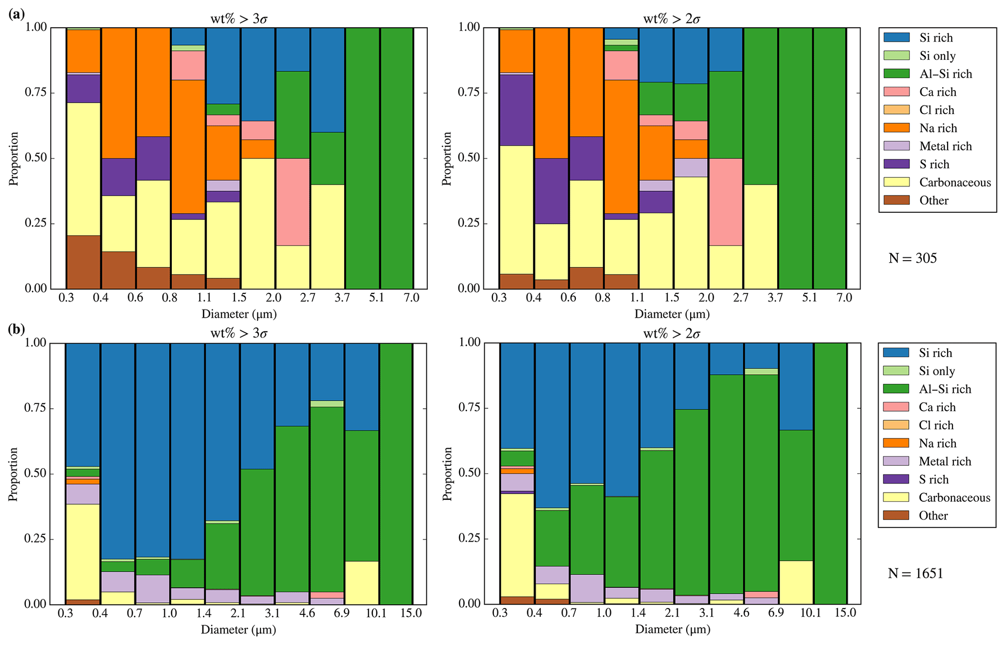
Figure C1 Size-segregated composition of two aerosol samples for different element detection confidence levels. The samples are 18 March 2018 from 19:28 to 19:48 UTC in northern Alaska (a) and 2 October 2017 from 16:24 to 16:40 UTC in Iceland (b). The two samples are very different since the first sample presented a very low aerosol loading and it is dominated by Na-rich particles and carbonaceous and mineral-origin aerosol (Si rich, Si only, Al–Si rich) with significant contributions of S-rich particles, whereas the second sample presented a high aerosol loading and it was mainly dominated by mineral-origin aerosol. The difference in the confidence mainly affected the Si- and Al–Si-rich particles as well as the S-rich particles in sample (a), whereas it only affected the Si- and Al–Si-rich particles in sample (b).