High-resolution temperature profiles retrieved from bichromatic stellar scintillation measurements by GOMOS/Envisat

In this paper, we describe the inversion algorithm for retrievals of high vertical resolution temperature profiles (HRTPs) using bichromatic stellar scintillation measurements in the occultation geometry. This retrieval algorithm has been improved with respect to nominal ESA processing and applied to the measurements by Global Ozone Monitoring by Occultation of Stars (GOMOS) operated on board Envisat in 2002–2012. The retrieval method exploits the chromatic refraction in the Earth's atmosphere. The bichromatic scintillations allow the determination of the refractive angle, which is proportional to the time delay between the photometer signals. The paper discusses the basic principle and detailed inversion algorithm for reconstruction of high-resolution density, pressure and temperature profiles in the stratosphere from scintillation measurements. The HRTPs are retrieved with a very good vertical resolution of ∼200 m and high precision (random uncertainty) of ∼1–3 K for altitudes of 15–32 km and with a global coverage. The best accuracy is achieved for in-orbital-plane occultations, and the precision weakly depends on star brightness. The whole GOMOS dataset has been processed with the improved HRTP inversion algorithm using the FMI's scientific processor; and the dataset (HRTP FSP v1) is in open access.

The validation of small-scale fluctuations in the retrieved HRTPs is performed via comparison of vertical wavenumber spectra of temperature fluctuations in HRTPs and in collocated radiosonde data. We found that the spectral features of temperature fluctuations are very similar in HRTPs and collocated radiosonde temperature profiles.

HRTPs can be assimilated into atmospheric models, used in studies of stratospheric clouds and used for the analysis of internal gravity waves' activity. As an example of geophysical applications, gravity wave potential energy has been estimated using the HRTP dataset. The obtained spatiotemporal distributions of gravity wave energy are in good agreement with the previous analyses using other measurements.

1 Introduction

This paper is dedicated to the description of a unique method for high-resolution temperature and density profiling using bichromatic satellite stellar scintillation measurements and to the assessment of the retrieved temperature profiles. The bichromatic stellar scintillation measurements were performed by two fast photometers at different wavelengths of the Global Ozone Monitoring by Occultation of Stars (GOMOS) instrument operated on board the Envisat satellite during 2002–2012 (https://earth.esa.int/web/guest/missions/esa-operational-eo-missions/envisat/instruments/gomos, last access: 17 January 2019; Bertaux et al., 2010). Before the description of the measurements and inversion algorithm, we give a precise definition what atmospheric parameter is retrieved (or measured).

1.1 What is a high-resolution temperature profile?

In the case of a HRTP (high-resolution temperature profile), the underlying atmospheric parameter that we aim to characterize is the temperature field. However, the temperature is a four-dimensional (4-D) scalar field, which is defined for each time moment over a 3-D space. Due to very active dynamical processes in the Earth's atmosphere, this 3-D field can contain significant fluctuations down to the viscous scale, which is typically smaller (and sometimes much smaller) than 1 m within the stratosphere and the troposphere.

During occultations, the velocity of the sounding ray within the atmosphere is much larger than the velocity of any atmospheric motion (for GOMOS/Envisat, it is more than 3000 m s⁻¹); therefore the “frozen-field” approximation during measurement time can safely be considered (Tatarskii, 1971). Regarding the spatial variation, the trace of the line of sight within the atmosphere during an occultation defines a 2-D surface, which differs only slightly from a plane because of refractive effects. The only temperature fluctuations able to affect the GOMOS measurements lie in this surface. Furthermore, since the signal recorded by a detector is intrinsically 1-D, the retrieved parameter (temperature or density) is also 1-D: it is roughly along the trajectory of the ray perigee point in the atmosphere.

Due to stable stratification of the stratosphere, most of the variations of meteorological parameters, such as the temperature, occur along the vertical direction. The field of temperature within the atmosphere is strongly anisotropic and the direction of its gradient is close to the vertical. Consequently, a measurement of temperature variations along the vertical direction, known as a “temperature profile”, describes most of the field variation within the considered region. However, the validity of the above statements is strongly dependent on the considered scale. Large-scale temperature fluctuations are strongly stratified (anisotropic); they contain the largest fraction of potential energy (or equivalently temperature variance). Most of the energetic dynamical processes, including meteorological flow and gravity waves, correspond to this anisotropic part. The characteristic ratio between dominant horizontal and vertical scales is typically equal to the ratio of maximal and minimal intrinsic frequencies of the gravity waves field. In the stratosphere, the ratio of buoyancy (Brunt–Väisälä) frequency N to the Coriolis parameter f, N∕f, is typically larger than 100 (Fritts and Alexander, 2003).

Small-scale fluctuations, mostly turbulence and, more generally, instable and dissipative processes, are much more isotropic (and so are the temperature gradients associated with such small-scale processes). For these kinds of fluctuations, the concept of a (vertical) profile is essentially meaningless. The transition between strongly anisotropic and roughly isotropic fluctuations occurs within the scale range separating the domains of waves and turbulence. For the stratosphere, it is roughly between 10 and 100 m of the vertical scale (Gurvich and Kan, 2003; Nastrom et al., 1997).

These general considerations about the structure of the atmospheric temperature field indicate that a 1-D “vertical profile” is only meaningful (for remote sensing measurements) for vertical scales larger than 30–100 m. The detailed characteristics of the measurement process must also be considered in order to grasp the real meaning of the retrieved profile and to better understand its relationship with the atmospheric temperature field. In the case of GOMOS, the concept of vertical profiles is adequate, as high-resolution temperature profiles, which will be discussed in our paper, have the vertical resolution of ∼200 m.

1.2 Bichromatic scintillation measurements by GOMOS and previous works on HRTPs

For retrievals of high-resolution temperature profiles, we use bichromatic scintillation measurements by the GOMOS fast photometers, which record the stellar flux with the sampling frequency of 1 kHz at blue (475–525 nm) and red (650–700 nm) wavelengths synchronously, as a star sets behind the Earth limb.

Two fast GOMOS photometers on board Envisat recorded the intensity fluctuations induced on the star's light by the refractivity fluctuations encountered within the atmosphere, at two wavelengths. A short description of the inversion algorithm for retrievals of high-resolution temperature profiles from bichromatic scintillation can be found in Dalaudier et al. (2006) and Sofieva et al.(2009c); it is also presented below in our paper.

The main advantage of a HRTP is its vertical resolution, which is ∼200–250 m. Such resolution allows probing gravity wave (GW) spectra. The validation of the small-scale structure of HRTPs is therefore an important issue before using the data in GW research. The validation of the small-scale structure is a challenging task because temperature fluctuations are rapidly varying due to gravity wave activity. Sofieva et al. (2008, 2009c) proposed the use of spectral analysis for the validation of small-scale structure in temperature profiles, as this approach allows the use of measurements separated by several hundreds of kilometers and by several hours. The previous validation has been performed on HRTPs processed by the FMI scientific processor (analogous to the ESA IPF v6 algorithm, with the same algorithm but with a slightly different retrieval grid and a different discretization of the Abel inversion) using collocated radiosonde data. It has been shown that the small-scale fluctuations in HRTPs have similar rms values as in collocated radiosonde profiles, for vertical (in orbital plane) occultations of bright stars (Sofieva et al., 2009c). In the case of oblique occultations or dim stars, the HRTP fluctuations are of larger amplitude than those of in situ measurements. An analogous study with the method of Sofieva et al. (2009c) but applied to much larger datasets of GOMOS HRTP IPF v6 and collocated radiosonde profiles has shown that fluctuations in HRTP v6 are nearly always larger than in the collocated radiosonde data (for both vertical and oblique occultations). Therefore, IPF v6 HRTP data were not recommended for gravity wave analyses. This will be illustrated and discussed in Sect. 4 of our paper.

Figure 1 Signals of red (FP2) and blue (FP1) GOMOS photometers.

In this paper, we introduce an improved version of the GOMOS HRTP algorithm and present the whole GOMOS HRTP dataset processed using the FMI's scientific processor, HRTP FSP v1. The basic principle of HRTP retrievals is described in Sect. 2. Section 3 is dedicated to a detailed description of the retrieval algorithm. Examples of retrieved HRTPs, their characterization and validation of the small-scale fluctuations are shown in Sect. 4. Illustrations of using HRTPs for gravity wave analyses are presented in Sect. 5. Summary and discussion conclude the paper in Sect. 6.

2 Basic principle of HRTP retrieval

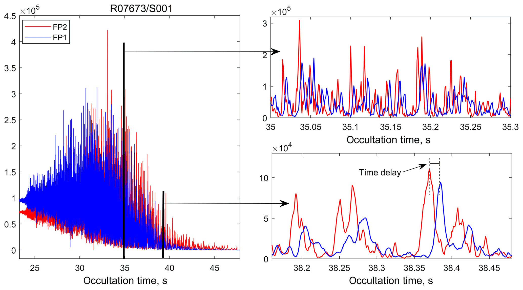
As discussed in Kyrölä et al. (2010) and Sofieva et al. (2009b), the light intensity transmitted through the atmosphere is affected not only by absorption and scattering, but also by refraction and diffraction. The scintillations (or large intensity fluctuations) observed at the satellite level are the result of the interaction of stellar light and atmospheric air density irregularities, which are generated mainly by internal gravity waves and turbulence. An example of scintillations recorded by GOMOS photometers is shown in Fig. 1.

The retrieval of HRTPs is based on the chromatic refraction in the atmosphere (Dalaudier et al., 2006). The refraction angle α depends on wavelength, due to the optical dispersion of air. For two rays of different color with the same impact parameter p (Fig. 2), the blue ray bends more than the red one (Fig. 2, α_B>α_R) and will consequently be observed later by GOMOS (only star settings are used in GOMOS observations). The scintillation spikes produced by atmospheric density fluctuations are observed by both photometers with a time delay t_B−t_R (Figs. 1 and 2), which is proportional to the refraction angle difference $\mathrm{\Delta }\mathit{\alpha }={\mathit{\alpha }}_{\mathrm{B}}-{\mathit{\alpha }}_{\mathrm{R}}$. The idea of such measurements of the refractive angle was first proposed by Gurvich and Sokolovskiy (1991, 1992).

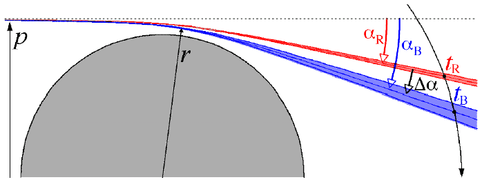
Figure 2 A scheme of chromatic refraction and the principle of refraction angle measurement by GOMOS. Both the refraction angles and the effect of dispersion are strongly exaggerated. However, the width of each beam relative to the angle difference Δα is realistic. The impact parameter p is the geometric distance of the ray from the Earth's center. The vertical separation of blue and red rays at the ray perigee of 30 km is ∼10 m (Dalaudier et al., 2001).

Using the accurate knowledge of the direction to the star and of the ENVISAT orbit, it is possible to convert the measured time delay into an angle difference Δα, and then into the refraction angle α at the reference wavelength (for GOMOS, the reference wavelength is 500 nm, i.e., α=α_B). The conversion factor is equal to ${\mathit{\alpha }}_{\mathrm{B}}/\mathrm{\Delta }\mathit{\alpha }={\mathit{\nu }}_{\mathrm{B}}^{\mathrm{0}}/\left({\mathit{\nu }}_{\mathrm{B}}^{\mathrm{0}}-{\mathit{\nu }}_{\mathrm{R}}^{\mathrm{0}}\right)\approx \mathrm{94}$, where ${\mathit{\nu }}_{\mathrm{0}}\left(\mathit{\lambda }\right)=n_{\mathrm{0}}\left(\mathit{\lambda }\right)-\mathrm{1}$ is the standard refractivity (n₀ is the refractive index) given for dry air at standard pressure and temperature (Edlén, 1966), and retractivities ${\mathit{\nu }}_{\mathrm{B}}^{\mathrm{0}}$ and ${\mathit{\nu }}_{\mathrm{R}}^{\mathrm{0}}$ correspond to central wavelengths of GOMOS photometers. After that, the method is similar to that used in radio occultation (e.g., Kursinski et al., 1997). Assuming local spherical symmetry of the atmosphere, the refractive index profile n(p) can be retrieved from the refraction angle profile α(p) using the Abel transform (Kursinski et al., 1997; Tatarskii, 1968):

$$\begin{array}{}\text{(1)}& \log \left(n\right(p\left)\right)={\displaystyle \frac{\mathrm{1}}{\mathit{\pi }}}\underset{p}{\overset{\mathrm{\infty }}{\int }}{\displaystyle \frac{\mathit{\alpha }\left(q\right)\mathrm{d}q}{\sqrt{q^{\mathrm{2}}-p^{\mathrm{2}}}}}.\end{array}$$

The tangent (or minimal) radius r is related to the impact parameter p through the refractive index n: $p=rn=rn\left(p\right(r\left)\right)$.

The refractivity profile $\mathit{\nu }\left(r\right)=n-\mathrm{1}$ can be easily converted into a density profile through $\mathit{\rho }\left(r\right)=\mathit{\nu }\left(r\right){\mathit{\rho }}_{\mathrm{0}}/{\mathit{\nu }}_{\mathrm{0}}$ using the conversion factor for dry standard air (15 ^∘C, 101 325 Pa). The corresponding pressure profile is reconstructed by integrating the hydrostatic equation, as is done in radio-occultation and lidar measurements (e.g., Hauchecorne and Chanin, 1980; Kursinski et al., 1997). Finally, the temperature profile T(r) is obtained from the state equation of a perfect gas.

3 From simplified theory to real experiment: HRTP processing algorithm

The main steps of processing the red and blue photometer signals to high-resolution temperature profiles can be outlined as follows:

• The chromatic time delay is estimated as the position of the maximum of the cross-correlation function of blue and red photometer signals after smoothing the red one. Since the refractive angle is proportional to chromatic time delay, the profile of the refractive angle is obtained.

• The refractivity profile is determined from the refractive angle profile via the Abel integral inversion. For upper limit initialization, an atmospheric model is used.

• The density profile is obtained from the refractivity profile using Edlén's formula.

• From the density profile, the pressure profile is calculated using the hydrostatic equation.

• Finally, the temperature profile is determined from these data using the state equation of a perfect gas.

Figure 3 (a) GOMOS optical filter response as a function of wavelength. (b) Refractivity bandwidth of the GOMOS optical filters.

This basic algorithm is given for a highly simplified situation. Below we present the detailed description of the most important inversion steps and discuss various effects which have occurred in the GOMOS experiment.

3.1 From photometer signals to the profile of time delay

The new HRTP processing starts at the altitude of 32 km, at which the time delay is larger than 1 ms and the scintillations are of large amplitude. In the previous retrievals, the upper altitude, at which the HRTP processing starts, depends on the strength of scintillation and value of a priori time delay τ_a (estimated using ECMWF analyses data). The sampling rate of GOMOS photometers allows determination of time delay up to ∼35–38 km. However, above 32 km, uncertainty of retrievals is large (see also discussion below); therefore the upper limit is set to 32 km in the new retrievals.

The bandwidth of GOMOS photometers is nearly the same in wavelength, but the refractivity bandwidths of photometer optical filters are significantly different (Fig. 3).

As a result, scintillation features are more smoothed in the blue signal than in the red one (Figs. 1, 2). In order to make the chromatic smoothing similar, the signal of red photometer is convolved with a Gaussian window G(t). The width of the smoothing window W_G is defined as a differential width of the blue and red signals for a Dirac perturbation in the refractive angle, $W_G^{\mathrm{2}}=W_{\mathrm{blue}}^{\mathrm{2}}-W_{\mathrm{red}}^{\mathrm{2}}$. It increases proportionally to the refractive angle as the line of sight deepens into the atmosphere and can be approximated as

$$\begin{array}{}\text{(2)}& W_G={\mathit{\alpha }}_{\mathrm{B}}L{\displaystyle \frac{\sqrt{\mathrm{\Delta }{\mathit{\nu }}_{\mathrm{0}\mathrm{B}}^{\mathrm{2}}-\mathrm{\Delta }{\mathit{\nu }}_{\mathrm{0}\mathrm{R}}^{\mathrm{2}}}}{{\mathit{\nu }}_{\mathrm{0}\mathrm{B}}}}{\displaystyle \frac{\mathrm{1}}{\mathrm{d}{h}_{\mathrm{d}}/\mathrm{d}t}},\end{array}$$

where Δν_0B is the variation of the standard refractivity corresponding to the spectral width Δλ_B of the blue photometer, Δν_0R is defined analogously for the red photometer, dh_d∕dt is the vertical velocity of the line of sight and L is the distance from the tangent point to the satellite.

Figure 4 (a) Maximum of cross-correlation function for two GOMOS occultations: R07673/S001 (64^∘ S 68^∘ W, β=23^∘, 19 August 2003 04:09:23 UTC), red line, and R07588/S002 (35^∘ S 135^∘ W $\mathit{\beta }=-\mathrm{2.6}$^∘ 13 August 2003 07:28:35 UTC), blue line. (b) Examples of cross-correlation functions at selected altitudes and their fit with the parabola (black and grey lines).

It is evident that the determination of time delay (as a function of time) by visual recognition of characteristic scintillation structures is not feasible. Therefore, the time delay is estimated via calculation of the cross-correlation function (CCF), followed by a determination of the position of its maximum. For computation of the CCF, photometer signals are cut into ∼50 % overlapping sections. The length of the sections should be chosen in order to contain a “sufficient” number of structures (scintillation spikes) while preserving the best available resolution for the angle profile. We found that the optimal length of segments τ_window corresponds to a vertical displacement of the line of sight within the atmosphere varying from 250 m at 32 km to 500 m at 5 km. The smoothed red signal is pre-shifted by the (smooth) a priori time delay τ_a rounded to the nearest millisecond (which will be hereafter referred to as a pre-shifted time delay) in order to best align with the blue signal. For computation of τ_a, we use ECMWF density data at the occultation location:

$$\begin{array}{}\text{(3)}& {\mathit{\tau }}_{\mathrm{a}}\left(t\right)=\mathit{\alpha }\left({\mathit{\lambda }}_{\mathrm{B}}\right)L{\displaystyle \frac{{\mathit{\nu }}_{\mathrm{0}\mathrm{B}}-{\mathit{\nu }}_{\mathrm{0}\mathrm{R}}}{{\mathit{\nu }}_{\mathrm{0}\mathrm{B}}}}{\displaystyle \frac{\mathrm{1}}{\mathrm{d}{h}_{\mathrm{d}}/\mathrm{d}t}}.\end{array}$$

The CCF is calculated with 1 ms resolution and the position of its maximum is searched around zero delay, in the range $\pm (\mathrm{0.1}{\mathit{\tau }}_{\mathrm{window}}+\mathrm{3})$ ms. The maximum point and its two neighbors are then interpolated using a parabola, which is the first approximation of the correlation function in the vicinity of its maximum. The examples of cross-correlation functions and their fits are shown in Fig. 4 (right) for two GOMOS occultations. The position of the maximum of the parabola is then added to the pre-shift in order to provide the time delay estimation for the corresponding scintillation sample.

Figure 5 Illustration of time delay regularization and retrievals based on occultation R07673/S001; red: pure measurements, blue: V6 regularization, green: new (Bayesian) regularization, black: a priori profiles (ECMWF). (a) Profile of cross-correlation coefficient C_max. (b) Profiles of time delay, (c) uncertainty of time delay (1σ), (d) measurement fraction and (e) retrieved temperature profiles and collocated sonde measurements at Marambio (magenta line).

Uncertainty of time delay determination depends on the shape of the cross-correlation function and on how accurate it is. The error in the determination of the position of the cross-correlation function maximum can be estimated as

$$\begin{array}{}\text{(4)}& {\mathit{\sigma }}_{\mathit{\tau }}\approx {\displaystyle \frac{\sqrt{\mathrm{2}}{\mathit{\sigma }}_{\mathrm{C}}}{\mathrm{\Delta }t{C}^{\prime \prime }\left({\mathit{\tau }}_{\mathrm{0}}\right)}},\end{array}$$

where $C^{\prime \prime }$ is the second derivative of the cross-correlation function of photometer signals at the point of its maximum, σ_C is the error (standard deviation) of the CCF and Δt is the discretization step (1 ms). The derivation of Eq. (4) uses Taylor expansion of the condition for the CCF maximum $C^{\prime }\left(\mathit{\tau }\right)=\mathrm{0}$ at the vicinity of the maximum τ₀ and the subsequent Gaussian error propagation. As follows from Eq. (4), uncertainty in determination of CCF maximum is proportional to the uncertainty of CCF values and depends on the shape of CCF: the broader the CCF, the larger the error. In assumption of a Gaussian distribution of intensity fluctuations, the cross-correlation coefficient C has an asymptotically Gaussian distribution with the standard deviation

$$\begin{array}{}\text{(5)}& {\mathit{\sigma }}_{\mathrm{C}}\approx {\displaystyle \frac{\mathrm{1}-C^{\mathrm{2}}}{\sqrt{n}}},\end{array}$$

where n is the sample size used in calculation of the cross-correlation coefficient. This approximation is valid for large samples. Finally, the error of time delay estimated can be written as

$$\begin{array}{}\text{(6)}& {\mathit{\sigma }}_{\mathit{\tau }}\approx {\displaystyle \frac{\sqrt{\mathrm{2}}(\mathrm{1}-C_{max}^{\mathrm{2}})}{C^{\prime \prime }\mathrm{\Delta }t\sqrt{n}}}.\end{array}$$

In Eq. (6), C_max is the maximum of the cross-correlation function, or the cross-correlation coefficient; $C^{\prime \prime }$ can be calculated from parameters of the parabolic fit. Due to assumptions made in deriving Eq. (6), it is clear that this formula only gives an approximate estimate for the error of time delay reconstruction.

The uncertainty of time delay increases at lower altitudes (Fig. 5c, red line) due to broadening of cross-correlation function (Fig. 4b). At some levels, correlation between photometer signals can be low due to the presence of turbulence, which leads to very uncertain time delay.

3.2 Regularization of time delay estimation

3.2.1 Motivation: influence of isotropic turbulence

The atmosphere contains small-scale turbulence producing nearly isotropic fluctuations of density. These fluctuations also produce scintillations during stellar occultations. The contribution of turbulence to the observed scintillations can be significant and sometimes even dominant (Sofieva et al., 2007a, b). The cross-correlation of bichromatic scintillations caused by isotropic turbulence is only significant when the chromatic separation distance of the ray trajectories does not exceed the Fresnel scale, which is ∼1 m for GOMOS (for illustration and more details, see Fig. 4 and the corresponding text in Sofieva et al., 2009b). The chromatic de-correlation for nearly vertical (in orbital plane) occultations is always small, while it can be significant in the case of oblique (off-orbital plane) occultations (Kan, 2004). On the other hand, the smoothing induced by the finite optical band of the photometers will selectively damp the fluctuations associated with turbulence in the vertical direction because of their smaller size. As a result, the cross-correlation between the two photometers has a minimum at some altitude depending on the obliquity of the occultation (hereafter we define the obliquity angle β as the angle between the direction of the apparent motion of the observed star and the local vertical at the ray perigee point; Gurvich and Brekhovskikh, 2001; Sofieva et al., 2007b). This is illustrated in Fig. 4a for the oblique occultation R07673/S001 with the obliquity angle β=23^∘. Strong turbulence is observed at upper altitudes, resulting in the drop of cross-correlation at 30–45 km. A more quantitative consideration of this effect is given in Kan (2004) and Gurvich et al. (2005). In some situations, the correlation between photometer signals is too low for an accurate determination of the time delay (Fig. 4a). These situations are handled through regularization applied to the time delay profile, which is described below.

3.2.2 Regularization algorithm

In the case of low correlation between the recordings of the fast photometers, the time delay determination as the position of the cross-correlation function maximum gives poor results, and it can induce unphysical fluctuations in the time delay profile.

In the V6 algorithm, the data points corresponding to low correlation between photometer signals (with cross-correlation coefficient CCC < 0.7) are replaced by the weighted mean of measured (obtained from cross-correlation) τ_meas and a priori (computed external data source, e.g., ECMWF analysis data) τ_a time delays:

$$\begin{array}{}\text{(7)}& \widehat{\mathit{\tau }}={\displaystyle \frac{{\mathit{\tau }}_{\mathrm{a}}/{\mathit{\sigma }}_{\mathrm{a}}^{\mathrm{2}}+{\mathit{\tau }}_{\mathrm{meas}}/{\mathit{\sigma }}_{\mathit{\tau }}^{\mathrm{2}}}{\mathrm{1}/{\mathit{\sigma }}_{\mathrm{a}}^{\mathrm{2}}+\mathrm{1}/{\mathit{\sigma }}_{\mathit{\tau }}^{\mathrm{2}}}}.\end{array}$$

The weights used in Eq. (7) are inversely proportional to the uncertainties of time delay ${\mathit{\sigma }}_{\mathit{\tau }}^{\mathrm{2}}$ (defined by Eq. 6) and the a priori profile ${\mathit{\sigma }}_{\mathrm{a}}^{\mathrm{2}}$. Hereafter, we will refer to this regularization as to the optimal filtering method. In the HRTP IPF v6 algorithm, the uncertainty of the a priori time delay is computed assuming that a priori air density has an uncertainty of 2.5 % below 25 km, 5 % at 35–50 km with the linear transition between these two altitude regions. The rationale of this approach was using the minimal a priori information in retrievals. The effects of optimal filtering on time delay, its uncertainty and the resulting temperature profile are illustrated in Fig. 5 by blue lines. As observed in Fig. 5, such filtering handles exceptional values, whereby the cross-correlation is low, but the resulting temperature profile has enhanced amplitude of temperature fluctuations at altitudes below 17 km compared to collocated sonde data. Validation of HRTPs, which have been processed with optimal filtering, against collocated radiosonde data (Sofieva et al., 2009c), has shown that the amplitude of temperature fluctuations in HRTPs is realistic for vertical occultations of bright stars (not affected by turbulence), but often excessive in oblique occultations.

In the new algorithm, we use the statistical optimization (Bayesian approach). It acts as a linear operator applied to the differences between measured and a priori time delays:

$$\begin{array}{}\text{(8)}& {\mathit{\tau }}_{\mathrm{reg}}={\mathit{\tau }}_{\mathrm{a}}+{\mathbf{C}}_{\mathrm{a}}{\left({\mathbf{C}}_{\mathrm{a}}+{\mathbf{C}}_{\mathrm{meas}}\right)}^{-\mathrm{1}}\left({\mathit{\tau }}_{\mathrm{meas}}-{\mathit{\tau }}_{\mathrm{a}}\right),\end{array}$$

where C_a is the covariance matrix of a priori time delay uncertainties and C_meas is the covariance matrix of measured time delay uncertainties. This formulation corresponds to the Bayesian estimator (maximum a posteriori method), provided measurement errors and a priori uncertainties have Gaussian distributions. The diagonal elements of C_a and C_meas are a priori and measured uncertainties (variance of the corresponding errors), while off-diagonal elements characterize the correlation length scale of measurements and a priori profiles. In the new algorithm, the correlation length for measurements is equal to the window used for computation of the cross-correlation function, while the correlation length of a priori profile is set to 2 times larger. The diagonal elements of C_a and C_meas are ${\mathit{\sigma }}_{\mathrm{a}}^{\mathrm{2}}$ and ${\mathit{\sigma }}_{\mathit{\tau }}^{\mathrm{2}}$, as in the optimal filtering. The covariance matrix of the regularized time delay is estimated as

$$\begin{array}{}\text{(9)}& {\mathbf{C}}_{\mathrm{reg}}={\left({\mathbf{C}}_{\mathrm{a}}^{-\mathrm{1}}+{\mathbf{C}}_{\mathrm{meas}}^{-\mathrm{1}}\right)}^{-\mathrm{1}}.\end{array}$$

With such an approach, the uncertain values of time delay are not replaced at selected altitudes like in the V6 algorithm, but according to length of photometer record used in the determination of time delay. The resulting time delay, its uncertainty and final temperature profile are illustrated in Fig. 5 (green lines). The resulting profile of time delay follows measurements in the stratosphere, while at lower altitudes, at which the uncertainty of measurements is large, it follows the a priori profile. The measurement fraction shown in Fig. 5d is defined as

$$\begin{array}{}\text{(10)}& \mathit{F}={\displaystyle \frac{{\mathbf{C}}_{\mathrm{a}}{\left({\mathbf{C}}_{\mathrm{a}}+{\mathbf{C}}_{\mathrm{meas}}\right)}^{-\mathrm{1}}{\mathit{\tau }}_{\mathrm{meas}}}{{\mathit{\tau }}_{\mathrm{reg}}}}.\end{array}$$

Division in Eq.(10) is element-wise. For the proposed algorithm, the measurement fraction is close to 1 in the stratosphere, while it decreases at altitudes below ∼20 km (green line in Fig. 5d). In the V6 algorithm, the measurement fraction is 1 (measurements only) if CCC > 0.7 and has sharp decreases from 1 at altitude layers with CCC < 0.7 (weighted mean of measurements and a priori values), as shown by the blue line in Fig. 5d.

The averaging kernel of the regularized time delay retrievals can be estimated in the classical way:

$$\begin{array}{}\text{(11)}& \mathbf{A}={\left({\mathbf{C}}_{\mathrm{a}}^{-\mathrm{1}}+{\mathbf{C}}_{\mathrm{meas}}^{-\mathrm{1}}\right)}^{-\mathrm{1}}{\mathbf{C}}_{\mathrm{meas}}^{-\mathrm{1}}.\end{array}$$

The examples of rows of the averaging kernel matrix A at selected altitudes are shown in Fig. 6 for the two occultations considered above: one oblique occultation, R07673/S001, with strong influence of isotropic turbulence, and another is the vertical occultation R07588/S002, with small influence of turbulence. The profiles of cross-correlation coefficients of photometer signals in these occultations are shown in Fig. 4. The averaging kernels are sharply peaked, and even more so for vertical occultations.

3.3 From time delay to refractive angle

Refractive angle is proportional to time delay between photometer signals. The proportionality coefficient depends on the difference in refractivity corresponding to the central wavelengths of photometers, distance from the ray perigee point to the satellite and the satellite velocity (Eq. 3). However, this simple relation is complicated by the fact that the stellar spectrum is modified by absorption and scattering during an occultation. As a result, the effective wavelength of the photometer signal varies with altitude. Knowing the stellar spectrum I(λ,t) measured through the atmosphere and the transmission functions f_filter(λ) of the photometer optical filter, it is possible to determine the effective wavelength:

$$\begin{array}{}\text{(12)}& {\mathit{\lambda }}_{\mathrm{eff}}\left(t\right)={\displaystyle \frac{\underset{{\mathit{\lambda }}_{min}}{\overset{{\mathit{\lambda }}_{max}}{\int }}\mathit{\lambda }I\left(\mathit{\lambda },t\right)f_{\mathrm{filter}}\left(\mathit{\lambda }\right)\mathrm{d}\mathit{\lambda }}{\underset{{\mathit{\lambda }}_{min}}{\overset{{\mathit{\lambda }}_{max}}{\int }}I\left(\mathit{\lambda },t\right)f_{\mathrm{filter}}\left(\mathit{\lambda }\right)\mathrm{d}\mathit{\lambda }}},\end{array}$$

where λ_min and λ_max correspond to the wavelength range of the optical filter.

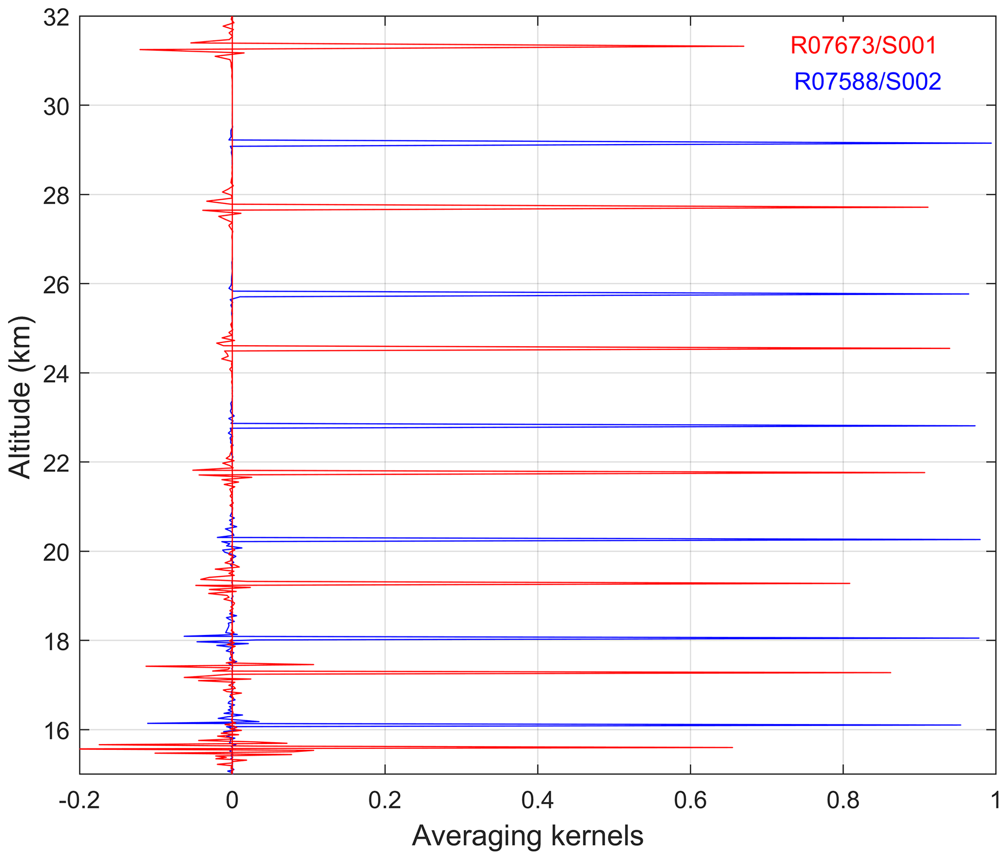
Figure 6 Examples of averaging kernels at selected altitudes, red: oblique occultation R07673/S001, blue: vertical occultation R07588/S002. The detailed information about these occultations can be found in the caption of Fig. 4.

Then the refractive angle α at the reference wavelength, which will be used in the further processing, can be computed as

$$\begin{array}{}\text{(13)}& \mathit{\alpha }={\displaystyle \frac{\mathit{\tau }}{L}}\mathrm{d}{h}_{\mathrm{d}}/\mathrm{d}t{\displaystyle \frac{{\mathit{\nu }}_{\mathrm{0}}\left({\mathit{\lambda }}_{\mathrm{ref}}\right)}{{\mathit{\nu }}_{\mathrm{0}}\left({\mathit{\lambda }}_{\mathrm{eff},\mathrm{blue}}\right)-{\mathit{\nu }}_{\mathrm{0}}\left({\mathit{\lambda }}_{\mathrm{eff},\mathrm{red}}\right)}}.\end{array}$$

Since the refractive angle is proportional to time delay, its uncertainty can be easily obtained by multiplication of the time delay uncertainty by the corresponding factor. The uncertainty associated with effective wavelength determination is negligible compared to time delay uncertainty.

3.4 From refractive angle to refractivity profile

By purely geometrical considerations and because the refractive angle is small, the impact parameter p for a given wavelength λ is given by

$$\begin{array}{}\text{(14)}& p(\mathit{\lambda },t)=h_{\mathrm{d}}\left(t\right)+\mathit{\alpha }\left(\mathit{\lambda },t\right)L\left(t\right).\end{array}$$

Applying the inverse Abel transform (Eq. 1), we can obtain the profile of refractive index n(p). The application of the Abel transform assumes local spherical symmetry of the atmosphere. This assumption is also used in retrievals from radio-occultation measurements. The error due to horizontal gradients of the refractive index at right angles to the direction of light propagation has been estimated in Healy (2001) and Sofieva et al. (2004); it is less than 1 % for altitudes above 10 km. The integration of Eq. (1) can be carried out numerically using any standard quadrature method. The weak singularity of the integrand at the lower limit does not cause problems for a numerical realization: the singularity can be estimated or the midpoint product integration method can be applied. The upper limit should be chosen high enough (∼120 km); therefore the refractive angle profile calculated using ECMWF analyses and MSIS90 (Hedin, 1991) data is used at altitudes above the HRTP range in the processing. Application of Abel integration requires a monotonic impact parameter. This requirement can be violated because the impact parameter is computed using the measured (noisy) refractive angle. In the current implementation, the impact parameter is computed using the smoothed refractive angle and its monotonicity is checked.

Real geometric (tangent) altitudes can be determined as

$$\begin{array}{}\text{(15)}& h={\displaystyle \frac{p}{n\left(p\right)}}-R,\end{array}$$

where R is the local radius of curvature of the Earth surface.

The error of refractivity reconstruction can be estimated using the matrix of the discretized Abel transform. Due to the fact that the Abel integral acts as a linear operator connecting refractive angle and refractivity, the covariance matrix of refractivity uncertainty C_ν can be estimated using the classical error propagation formula:

$$\begin{array}{}\text{(16)}& {\mathbf{C}}_{\mathit{\nu }}={\mathbf{AC}}_{\mathit{\alpha }}{\mathbf{A}}^T,\end{array}$$

where A is the matrix of the discretized Abel transform (see, e.g., Sofieva and Kyrölä, 2004) and C_α is the covariance matrix of refractive angle uncertainties.

3.5 From refractivity to density, pressure and temperature

The density profile can be obtained from the refractivity profile using Edlén's formula. By using the hydrostatic equation we can calculate the pressure P at the altitude h as

$$\begin{array}{}\text{(17)}& P\left(h\right)=\underset{h}{\overset{\mathrm{\infty }}{\int }}g\left(x\right)\mathit{\rho }\left(x\right)\mathrm{d}x,\end{array}$$

where g(x) is the acceleration of gravity. The high-altitude initialization of pressure is obtained from an external model.

Finally, temperature can be determined from the equation of the state of a perfect gas:

$$\begin{array}{}\text{(18)}& T={\displaystyle \frac{M}{R}}{\displaystyle \frac{P}{\mathit{\rho }}},\end{array}$$

where R=8.3144 J mol⁻¹ K⁻¹ is the universal gas constant and M is the molar mass of dry air.

The covariance matrix of air density errors C_ρ is proportional to the covariance matrix of refractivity errors C_ν (relative errors are equal).

Two main terms contributing to the error in temperature are the error in local density (small-scale structures in density and temperature are anti-correlated and of equal relative amplitudes) and the error in pressure at the top of the high-resolution profile P_top (error of upper limit initialization). They are added quadratically, thus giving the uncertainty of the HRTPs:

$$\begin{array}{}\text{(19)}& {\left({\displaystyle \frac{\mathrm{\Delta }T}{T}}\right)}^{\mathrm{2}}={\left({\displaystyle \frac{\mathrm{\Delta }\mathit{\rho }}{\mathit{\rho }}}\right)}^{\mathrm{2}}+{\left({\displaystyle \frac{\mathrm{\Delta }{P}_{\mathrm{top}}}{P_{\mathrm{top}}}}{\displaystyle \frac{P_{\mathrm{top}}}{P}}\right)}^{\mathrm{2}}.\end{array}$$

In HRTP retrievals, the vertical resolution is defined mainly by the length of scintillation records that are used for calculation of the cross-correlation function, which is ∼250 m. Due to using overlapping samples, the actual vertical resolution is somewhat smaller. The regularization on time delay can slightly degrade the vertical resolution in the case of oblique occultations as illustrated in Fig. 6. Other inversion steps from time delay to temperature profile also degrade the vertical resolution (e.g., Sofieva and Kyrölä, 2004), but this degradation is minor and the main vertical resolution limitations are in time delay estimation. Therefore, overall vertical resolution of HRTPs is expected to be close to 250 m. In our validation analyses presented in Sect. 4 we assess this estimate.

4 Retrieved HRTPs, their characterization and validation

Examples of retrieved GOMOS high-resolution temperature profiles are shown in Figs. 7 and 8 by red lines with 1σ uncertainties (shaded area; all uncertainties presented in our paper are 1σ). In Fig. 7, HRTPs are for bright stars in vertical occultations (the best data quality), while in Fig. 8 other occultations are illustrated (oblique or of dim stars). These temperature profiles are collocated with high-resolution radiosonde data from the SPARC data center (https://www.sparc-climate.org/data-centre/data-access/us-radiosonde/, last access: 21 January 2019). In our illustrations and validation analyses, we use radiosonde data from the US high-resolution radiosonde archive, which contains data from 93 US-operated stations from the years 1998 to 2011. The stations are located across the mainland US, Alaska, Pacific islands and the Caribbean. Most of the data are in 6 s temporal resolution (the vertical resolution is ∼30 m), but in recent years, the stations have been upgraded to provide data in 1 s resolution.

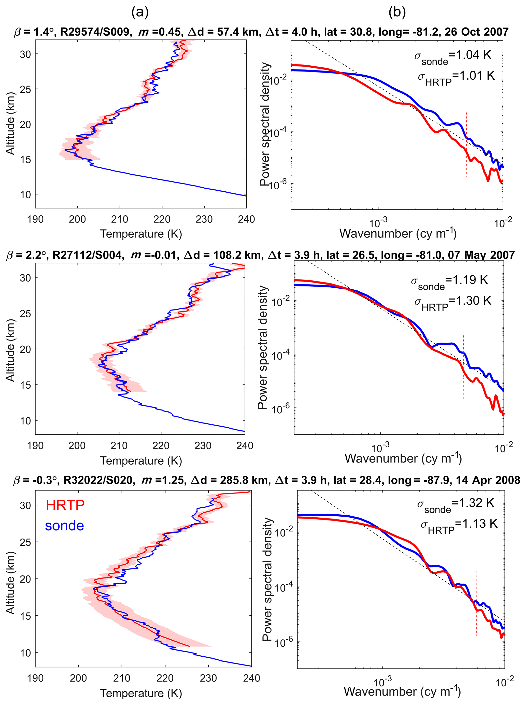
Figure 7 (a) Examples of HRTPs and collocated radiosonde profiles for some full-dark vertical occultations of very bright stars: (b) power spectral densities for these profiles, for the altitude range 18–30 km. Dashed black lines show the spectra corresponding to the saturated gravity wave model with the slope of −3 (Smith et al., 1987). Information about GOMOS measurements, obliquity angles β, star magnitude m, spatial Δd and temporal Δt separation, as well as the values of rms fluctuations are specified above each panel. Red dashed vertical lines in right-hand panels indicate the small-scale regions where HRTP resolution can affect the spectra.

Figure 8 As Fig. 7, but for oblique occultations and/or dim stars.

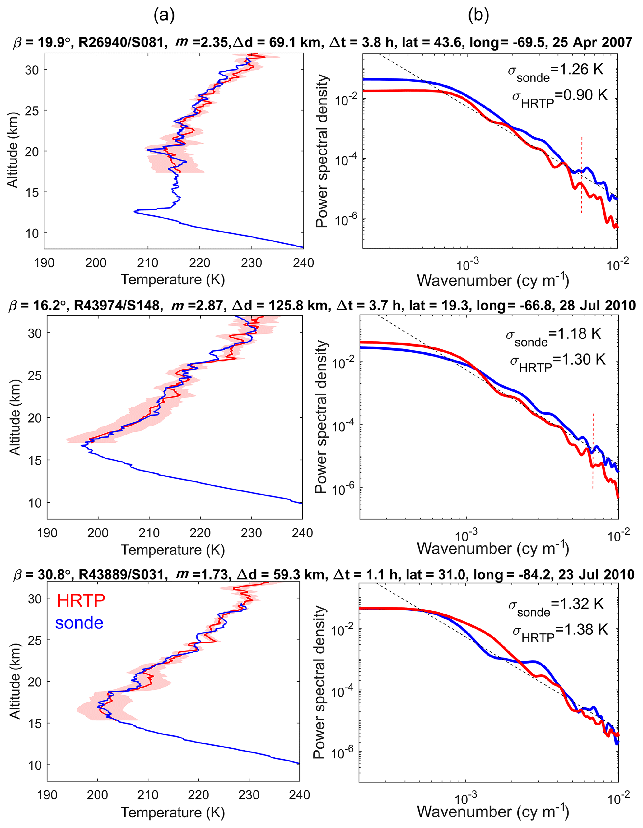
The collocated temperature profiles are shown by blue lines in the left-hand panels of Figs. 7 and 8, and information about the spatiotemporal difference is provided in the figure. We would like to note that the fine structure in the HRTPs and radiosonde profiles is not expected to coincide because of the evolution of the gravity wave field in the space–time window. For similarity of temperature profiles, including their small-scale fluctuation, the horizontal separation should be ideally less than 20 km and the time difference should not exceed 2–3 h, as discussed in Sofieva et al. (2008, 2009c). The time separation results in additional spatial separation in the atmosphere caused by advection of air masses. The relatively long measurement time of temperature profiles by radiosondes during balloon flights (it takes ∼1 h for the balloon to rise to 10–30 km) has a similar effect (the quantitative estimates of these effects can be found in Sofieva et al., 2009c). In the left-hand panels of Figs. 7 and 8, the HRTPs and collocated radiosonde profiles are similar, but not fully coinciding, as expected. The temperature profiles for the vertical occultation of bright stars are of a similar quality as for other occultations, as demonstrated by a comparison of Figs. 7 and 8.

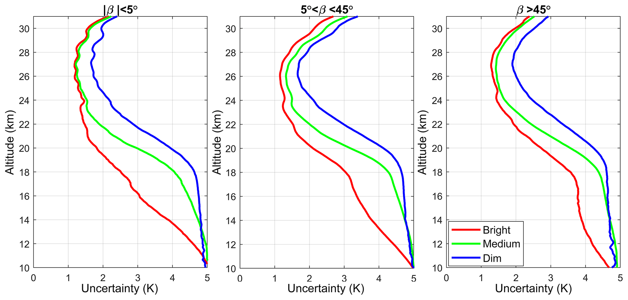
Figure 9 Mean uncertainties of HRTPs in the equatorial region (20^∘ S–20^∘ N) in 2004, for different obliquity angles β, specified in the panels, and for different stars: bright (m<1), medium ($\mathrm{1}<m<\mathrm{2.5}$) and dim (m>2.5).

Despite differences in small-scale temperature fluctuations, we can expect similar spectral properties of the temperature field at locations not far from each other (e.g., less than 500 km) during some time period (a few hours), as shown in Sofieva et al. (2008). The power spectra density of relative temperature fluctuations in HRTPs and collocated radiosonde profiles are shown in the right-hand panels of Figs. 7 and 8. For the spectral analysis, the collocated profiles were interpolated to an equidistant altitude grid with a 30 m resolution in the altitude range 18–30 km. Hanning filtering with a 3 km cutoff scale was used to obtain the smooth component. One can notice a good agreement of wavenumber spectra of HRTP and radiosonde temperature fluctuations, for all the considered GOMOS occultations. In contrast to the previous HRTP validation results (Sofieva et al., 2009c), the spectra of temperature fluctuations are also similar in the case of oblique occultation or dim stars.

The HRTP wavenumber spectra in Figs. 7 and 8 have visible cutoffs corresponding to scales ∼150–250 m (these regions are indicated by vertical red dotted lines). This is the experimental conformation of the vertical resolution of HRTPs ∼250 m. This agrees with the theoretical estimates of the HRTP retrievals (it is defined mainly by the lengths of the scintillation records used for evaluation of the time delay).

Typical estimated (in the retrieval algorithm) uncertainties of HRTP retrievals are shown in Fig. 9, for occultations of different types. The HRTPs are considered in the equatorial region (20^∘ S–20^∘ N; tropopause is ∼18 km) in 2004. As seen in Fig. 9, the estimated HRTP uncertainty is 1–3 K in the stratosphere, at altitudes from ∼2 km above the tropopause to ∼30 km. The best quality is achieved in vertical occultations. The uncertainty of the retrievals depends weakly on star brightness; it is only noticeably larger for occultations of dim stars with visual magnitude m > 2.5.

In this paper, we focus on the validation of small-scale fluctuations in HRTPs, as the HRTP vertical resolution allows gravity waves to be probed. Following Sofieva et al. (2008, 2009c), we use spectral analysis for validation of the small-scale structure in temperature profiles, as this approach allows measurements to be used that are separated by several hundreds of kilometers and by several hours. This study applies the method by Sofieva et al. (2009c) to much larger datasets of HRTPs and collocated radiosonde profiles. In our illustrations, the 1 s data from the SPARC data center archive, which is described above, are used. However the US 6 s data and other high-resolution radiosonde datasets obtained from NDACC, NILU, SHADOZ and the Sodankylä radiosonde station are also analyzed and they show similar results. The collocated HRTP and radiosonde data are selected using 300 km and a 4 h space–time window. With this criterion, 5023 collocated profiles are found in the 6 s resolution dataset and 1070 in the 1 s resolution data. Among the collocated data, there are occultations of different types.

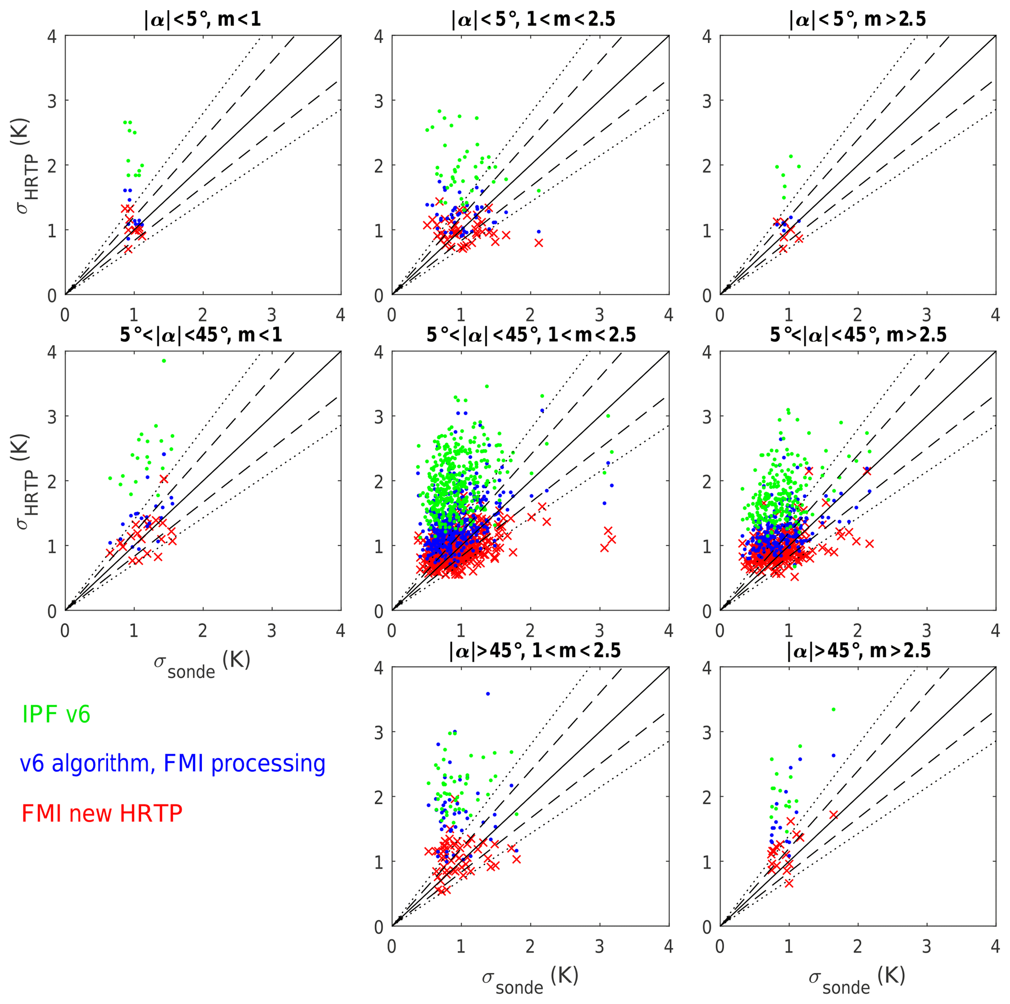
Figure 10 Standard deviations of temperature fluctuations in the altitude range 18–30 km for occultations of different types (see text for explanation). Processing version: IPF V6 (green), the V6 algorithm implemented in the FMI scientific processor (blue) and the new HRTP-FMI algorithm (red). Dashed black lines: y=1.2x and $y=(\mathrm{1}/\mathrm{1.2})x$; solid black lines: y=1.4x and $y=(\mathrm{1}/\mathrm{1.4})x$.

Keeping in mind the results of the previous validation, we compared the rms values of temperature fluctuations in radiosonde temperature profiles with those in HRTPs, in the altitude range 18–30 km, for different occultation types, vertical (|β|<5^∘), of medium obliqueness ($\mathrm{5}{}^{\circ }<\mathit{\beta }<\mathrm{45}$^∘) and highly oblique (β>45^∘), and for stars of different brightness, bright (visual magnitude m<1), of medium brightness ($\mathrm{1}<m<\mathrm{2.5}$) and dim (m>2.5). We detected fluctuations about the smooth profile, which was computed from the original profiles using a Hanning filter with the 3 km cutoff scale. The rms values of temperature fluctuations in collocated HRTP and radiosonde data, σ_hrtp and σ_sonde, respectively, are presented as scatter plots (Fig. 10). The colored markers in Fig. 10 correspond to different versions of HRTP processing: IPF v6 (green), v6 algorithm implemented in FMI scientific processor (blue) and the new HRTP algorithm presented in this paper (red). We found that the rms of HRTP v6 fluctuations is overall larger than that in collocated radiosonde profiles for all occultation types, despite the fact that the vertical resolution is finer for radiosonde data (and thus the opposite behavior is expected). However, the v6 algorithm implemented in the FMI HRTP scientific processor shows behavior consistent with the previous analysis of Sofieva et al. (2009c): the small-scale fluctuations in HRTPs are realistic for vertical occultations of bright stars, and the HRTP fluctuations are of larger amplitude than in collocated radiosonde temperature profiles in the case of oblique occultations or dim stars. For the new HRTP retrieval algorithm, σ_hrtp and σ_sonde are similar for all occultation types. This demonstrates a clear improvement of new HRTP data.

Several examples of wavenumber spectra of relative temperature fluctuations are shown in Figs. 7 and 8, which show quite typical behavior: the spectra are similar for HRTPs and collocated radiosonde profiles.

5 Illustrations of HRTP application: GW potential energy

In this section, we show illustrations of applications of HRTPs for analyses of gravity waves. The spatiotemporal distributions are presented only to demonstrate that the new HRTP dataset provides valuable geophysical information, which is in agreement with analyses using other datasets.

Figure 11 GW potential energy in two seasons, in the years 2002–2011.

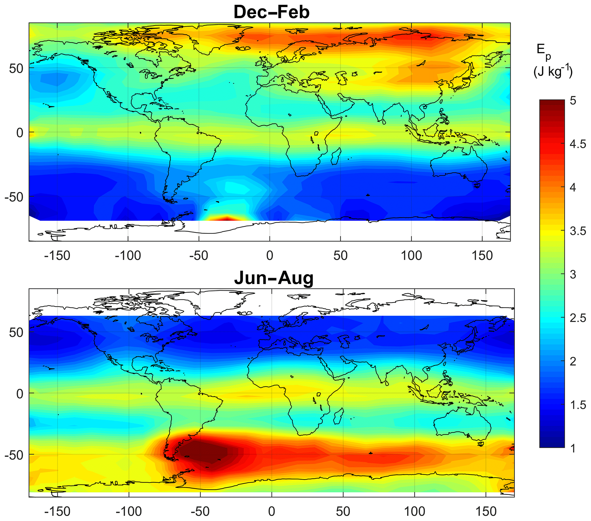
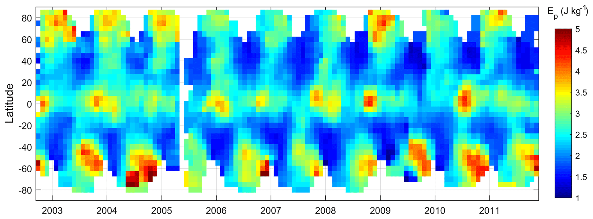
Figure 12 Time series of GW potential energy (zonal average) estimated from GOMOS HRTPs in the years 2002–2011.

The gravity wave potential energy per unit mass is defined as

$$\begin{array}{}\text{(20)}& E_{\mathrm{P}}={\displaystyle \frac{\mathrm{1}}{\mathrm{2}}}{\displaystyle \frac{g^{\mathrm{2}}}{N^{\mathrm{2}}}}〈{\left({\displaystyle \frac{\mathit{\delta }T}{T_{\mathrm{s}}}}\right)}^{\mathrm{2}}〉,\end{array}$$

where $\frac{\mathit{\delta }T}{T_{\mathrm{s}}}$ is the relative temperature fluctuations with respect to the smooth (background) profile T_s, and g is the acceleration of gravity.

In our analysis, smooth profile T_s is obtained by smoothing HRTPs down to 4 km resolution. The Brunt–Väisälä frequency N² is estimated using the smoothed HRTP. The GW potential energy has been evaluated for each temperature profile in the altitude range 20–30 km.

Figure 11 shows the distribution of GW energy in two seasons, winter and summer. These distributions are evaluated using individual E_P values averaged in 10^∘ latitude × 20^∘ longitude bins, for the whole GOMOS dataset from 2002 to 2011. The distributions of E_P shown in Fig. 11 are in very good agreement with previous estimates of this parameter from radiosonde, lidar and GPS radio-occultation measurements, both qualitatively and quantitatively (Allen and Vincent, 1995; de la Torre et al., 2006; Sofieva et al., 2009a; Tsuda et al., 1991, 2000). The overall distribution reproduces the known features: strong GW activity close to the edge of polar vortex and a peak near the Antarctic Peninsula in local winter. Enhancements in equatorial regions are clearly observed, analogous to those found in global analyses of radio-occultation data (de la Torre et al., 2006; Tsuda et al., 2000).

Temporal evolution of GW potential energy, for different latitudes, is shown in Fig. 12. This time series is very similar to that shown in de la Torre et al. (2006, Fig. 1) obtained from radio-occultation data. Enhancements at polar and midlatitudes in winter are observed; they are larger in the Southern Hemisphere and follow the evolution of the polar night jet (de la Torre et al., 2006; Sofieva et al., 2009a). The enhancement in the equatorial region is also observed, which seems to be annual but might also be modulated by quasi-biennial oscillations. Similar equatorial enhancements are observed by de la Torre et al. (2006).

We would like to note that, despite similarities of the GW energy morphology presented in our paper with the previous studies, there are expectedly some differences and peculiar features because contributions of small-scale gravity waves (down to 250 m vertical scale) are also present in HRTPs. Detailed analyses of gravity wave distributions using HRTPs might be the subject of future works and publications.

6 Summary and discussion

We described the improved algorithm for high-resolution temperature and air density profiling using bichromatic scintillation measurements. This method allows temperature profiling in the altitude range 10–32 km with a vertical resolution of ∼250 m and accuracy in the stratosphere of 1–3 K. The main difference of the FSP v.1 retrieval algorithm compared to ESA nominal processing is the Bayesian regularization of time delay profiles, which improves retrievals for oblique occultations and at lower altitudes. The retrieval algorithm is applied to the whole GOMOS/Envisat dataset, and the new GOMOS HRTP FSP v1 dataset is now available. The best accuracy is achieved for vertical occultations of bright stars. The uncertainty of HRTP retrievals depends weakly on stellar brightness.

The spectral analysis of HRTPs and collocated radiosonde profiles has been applied for validation of small-scale fluctuations. It has been shown that the HRTP fluctuations are realistic (in terms of their 1-D vertical spectra), for all types of occultations.

The main factors limiting accuracy of HRTP retrievals are due to instrumental properties in combination with the specifics of refraction in the Earth atmosphere. In general, the upper limit of HRTPs is defined mainly by the sampling frequency of the photometers: the detectable time delay should be larger than the photometer integration time, 1 ms; it is usually below 35–37 km. For faster photometers and larger wavelength separation, the upper limit can be higher. The presence of uncorrelated scintillations generated by locally isotropic turbulence reduces the useful information content in the photometer data. At lower altitudes, the influence of isotropic turbulence is low due to selective filtering by the photometer optical filters. However, a lower signal-to-noise ratio at lower altitudes due to the influence of absorption and broadening of scintillation peaks due to chromatic smoothing degrade the accuracy of HRTP retrievals at altitudes below 15–17 km. Narrower optical filters would allow slightly better retrievals at lower altitudes. The physical model for HRTP retrievals is adapted for vertical and moderately oblique occultations (for which tan(β) is smaller than anisotropy of air density irregularities). Such occultations constitute the majority of GOMOS measurements. The crossing of rays (strong scintillation) at low altitudes is not taken into account by the model. However, its influence is reduced due to the spatiotemporal averaging by the GOMOS optical filters (Kan et al., 2001), thus also allowing acceptable temperature retrievals from GOMOS scintillation measurements at altitudes below 25 km.

HRTPs can be assimilated into atmospheric models, used in studies of stratospheric clouds and used in analysis of internal gravity wave activity. As an illustration of application of HRTPs for gravity wave research, GW potential energy has been evaluated using the GOMOS HRTP dataset. The obtained spatiotemporal distributions of GW potential energy are in good agreement with previous analyses using other datasets.

This paper is dedicated mainly to the retrievals, validation and geophysical assessment of small-scale fluctuations in the retrieved GOMOS high-resolution temperature profiles. However, HRTPs can be smoothed down to lower resolution, and used in other analyses, including analyses of temperature trends, with a combination of 10-year GOMOS HRTP data and other limb profile temperature measurements. This could be a subject of future research.