Multiple-scattering correction factor of quartz filters and the effect of filtering particles mixed in water: implications for analyses of light absorption in snow samples

The deposition of light-absorbing aerosol (LAA) onto snow initiates processes that lead to increased snowmelt. Measurements of LAA, such as black carbon (BC) and mineral dust, have been observed globally to darken snow. Several measurement techniques of LAA in snow collect the particulates on filters for analysis. Here we investigate micro-quartz filters' optical response to BC experiments in which the particles are initially suspended in air or in a liquid. With particle soot absorption photometers (PSAPs) we observed a 20 % scattering enhancement for quartz filters compared to the standard PSAP Pallflex filters. The multiple-scattering correction factor (C_ref) of the quartz filters for airborne soot aerosol is estimated to be ∼3.4. In the next stage correction factors were determined for BC particles mixed in water and also for BC particles both mixed in water and further treated in an ultrasonic bath. Comparison of BC collected from airborne particles with BC mixed in water filters indicated a higher mass absorption cross section by approximately a factor of 2 for the liquid-based filters, which is probably due to the BC particles penetrating deeper in the filter matrix. The ultrasonic bath increased absorption still further, roughly by a factor of 1.5, compared to only mixing in water. Application of the correction functions to earlier published field data from the Himalaya and Finnish Lapland yielded mass absorption coefficient (MAC) values of ∼7–10 m² g⁻¹ at λ=550 nm, which is in the range of the published MAC of airborne BC aerosol.

1 Introduction

Soot refers to carbonaceous particles formed during the incomplete combustion of hydrocarbon fuels and includes black carbon (BC) and organic carbon (OC) but can also include other elements, such as sulfates. As the most light-absorbing aerosol (LAA) by unit of mass, BC is highly efficient in absorbing solar radiation and is a vital component in Earth's radiative balance (Bond et al., 2013). Once the particles are scavenged from the atmosphere, possibly far from their emission source, BC can reach the snow surface and decrease the snow reflectivity (Warren and Wiscombe, 1980; Flanner et al., 2007). This will lead to accelerated and increased snowmelt, observed in different snow environments across the globe (see, e.g., recent review by Skiles et al., 2018). Perhaps the most notable is high-mountain Asia and its extensive cryosphere, where large emission sources of LAA in close proximity are affecting the region's snow and ice (e.g., Xu et al., 2009; Gertler et al., 2016; Zhang et al., 2017).

Figure 1 Experimental setup for the airborne (a) and for the liquid (b) procedures.

There are a variety of methods for measuring BC, which is reflected in BC being operationally defined. A common practice is to measure the change in transmission of a filter collecting aerosol. The measured signal (i.e., optical depth of the filter) is thereafter applied with correction factors to generate atmospheric concentrations of so-called equivalent black carbon (eBC) according to the BC nomenclature (Petzold et al., 2013). The correction factors account for (1) the loading of aerosol on the filter since the detection signal decreases with increased aerosol content, (2) the multiple scattering of light that is enhanced in the filter substrate, and (3) the enhancement from the deposition of other light-scattering aerosol. One instrument used for light absorption measurements is the particle soot absorption photometer (PSAP), utilizing Pallflex filters. As an alternative to the optical filter analysis of eBC, another approach is to apply the thermal–optical method (TOM), providing organic carbon (OC) and elemental carbon (EC) mass of the aerosol on the filter. With this method, EC refers to the carbon content of carbonaceous matter (Petzold et al., 2013) and can be assumed to be the main light-absorbing element of BC. The technique involves a stepwise heating procedure, therefore creating a need to use micro-quartz-fiber filters. These filters have been used in numerous studies with filtering snow and ice samples and have been analyzed thereafter to determine the EC and OC content of the samples (e.g., Hagler et al., 2007; Forsström et al., 2009; Meinander et al., 2013; Ruppel et al., 2014; Zhang et al., 2017). In Svensson et al. (2018), measurements with TOM were combined with an additional transmittance measurement to further investigate the relative contribution from BC and other LAA particles present in snow samples. The study involved laboratory tests as well as comparisons to ambient snow samples taken from different environmental settings. One lesson from this study was that the optical properties of absorbing particles on quartz filters must be better understood, in particular when using melted snow samples.

The overarching goal of this paper is to further investigate micro-quartz-fiber filters' optical behavior when sampling BC particles in a liquid (to simulate snow sampling). An advantage of using these filters is that the sample can be analyzed readily using TOM to reach an EC concentration on the filter (where MAC values are not needed). The aim is pursued through a series of laboratory studies. Our approach is to compare the use of quartz-fiber filter for air and liquid samples to the much better characterized Pallflex type filer used in commercial PSAPs. Hence, we do not intend to determine a universal MAC value but rather to understand differences in the observations that might be due to the filter substrate or handling of the sample. We do not intend to answer all possible issues with filter sampling but will concentrate on the difference using the two filter types in air samples, the difference between air and liquid samples with respect to the quartz-fiber filter, and finally the potential effect from treating the liquid samples using ultrasound.

2 Materials, instruments, and data analyses

2.1 Soot aerosol production and sampling

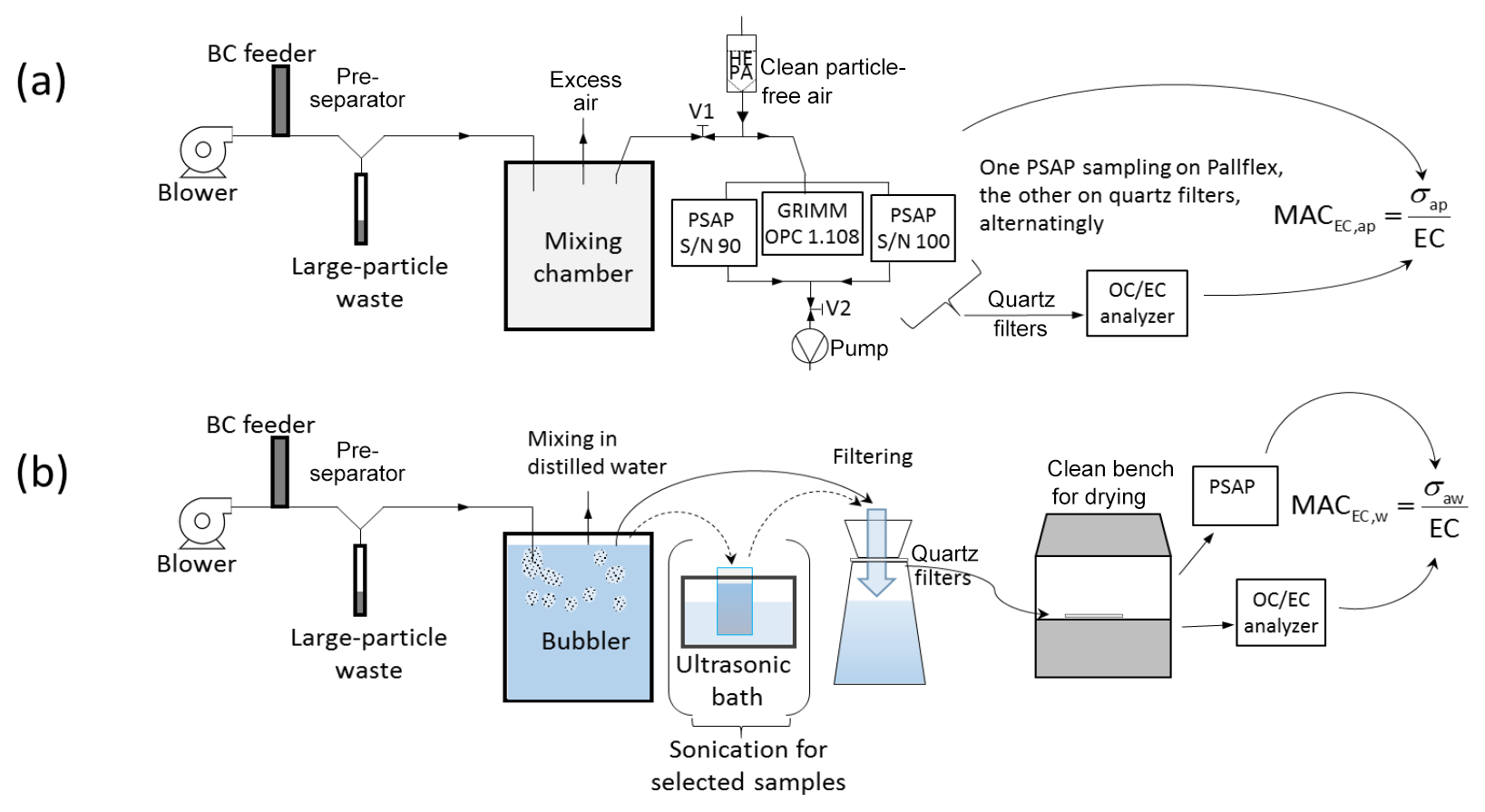
A schematic picture of the experiment is presented in Fig. 1, and the methods used in each step are outlined in the Sect. 2.1.1 and 2.1.2 below as well as the instrumentation used (Section 2.2). Section 2.3 explains the data processing. The soot used consisted of particles collected by chimney cleaners in Helsinki, Finland, and this particular soot batch is from small-scale oil-based burning. The same soot has been applied in different experiments previously (Peltoniemi et al., 2015; Svensson et al., 2016, 2018).

2.1.1 Airborne sampling

Soot aerosol was sampled onto filters in an airborne phase and as a part of liquid solution. In the airborne aerosol tests, soot was blown into a cylindrical experimental chamber (0.8 m height × 0.45 m diameter) through a stainless-steel tube (25 mm outer diameter) consisting of a y-shaped bend of 130^∘, creating a size separation of the aerosol. Essentially a virtual impactor, this setup allowed the smaller-sized particles to continue with the airflow into the chamber, while the larger (and heavier) particles were deposited into a waste pipe through inertial separation (see Sect. 2.2.3 for further description and results in Sect. 3.1.1). From the experimental chamber a sample inlet (copper, 6 mm outer diameter) simultaneously fed two PSAPs and a portable aerosol spectrometer (Grimm 1.108). One of the PSAPs had quartz-fiber-filter punches mounted, while the other had standard PSAP filters installed. This setup was alternated among the PSAPs in between the experimental runs during the experiment to have both PSAPs assessed with the different filters. In total, 22 different experimental rounds were made with various amounts of aerosol deposited to the substrates.

2.1.2 Liquid sampling

In the liquid experiments, the same soot batch and procedure were used as above, but the outlet pipe was submerged into a 20 L container filled with deionized, purified Milli-Q (MQ) water. From this liquid solution, different small amounts (between 10 and 100 mL) were extracted and mixed with additional MQ water to further dilute the sample (to a typical total volume of 400 mL). This was performed to get a range of filters with different EC concentrations and optical depths. The total number of liquid-generated filters was 35. Some selected liquid samples (n=10) were exposed to an ultrasonic bath (for at least 15 min) prior to filtration. All of the liquid solutions were filtered onto the same quartz filters used in the airborne test, applying the same filtering principles and analysis procedures as used previously (Svensson et al., 2018). Punches from dried filters had their transmittance first measured using a PSAP, followed by EC concentration measurements (TOM). This procedure was also applied to the quartz filters from the airborne experiment.

2.2 Instruments

2.2.1 Absorption measurements

Absorption was measured with two Radiance Research three-wavelength PSAPs (S/N 90 and S/N 100) at λ=467, 530, and 660 nm (Virkkula et al., 2005). One of them was loaded with a Pallflex E70-2075W filter that is generally used with the instrument, while the other was loaded with micro-quartz-fiber filters (Munktell, grade T293). The flows were calibrated with a Gilian Gilibrator bubble flow meter and set to 0.5 L min⁻¹. Higher flow rates were not used here, since the quartz filter tends to be more fragile and may not withstand higher flows. The sample spot diameters of the PSAPs were measured with an Eschenbach scale loupe with a 0.1 mm graduation 10 times each. The average diameters (± standard deviation) were 5.04±0.10 and 5.05±0.10 mm, giving corresponding spot areas of 19.9±1.6 and 20.0±1.6 mm². The aim was to use identical face velocities, i.e., average velocity of aerosol perpendicular to the filter (e.g., Müller et al., 2014) through both filter materials. The essentially identical spot areas also meant that we had tuned the flow rates identically. In addition, to study whether the PSAPs themselves affect the results, we used both filter materials alternatingly, as mentioned above, resulting in half of the 22 quartz filter samples being collected on the PSAP S/N 100 and the other half on the PSAP S/N 90. Another custom-built one-wavelength PSAP (λ=526 nm; Krecl et al., 2007) used in Svensson et al. (2018) was also utilized in for transmittance analysis of all the filters after their production in the airborne and liquid experiments.

2.2.2 EC measurements

Punches (typically with an area of 0.64 cm²) taken from the quartz filters were determined for their OC and EC content with a Sunset Laboratory OCEC analyzer (Birch and Cary, 1996), using the EUSAAR 2 protocol (Cavalli et al., 2010). The analysis procedure is based on stepwise increases in temperature in a helium atmosphere for the first stage, during which OC is detected with a flame ionization detector. The second phase of the analysis consists of introducing oxygen into the temperature increases and the detection of EC. Pyrolysis of OC during the first phase is monitored by a continuous laser transmittance measurement. Once the transmittance has reached the initial value for the filter in the second phase, a separation split point between OC and EC is established.

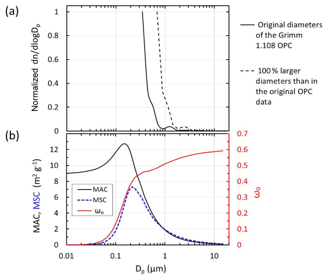
Figure 2 Size-dependent aerosol properties relevant to the experiment. (a) Normalized average particle number size distribution of soot aerosol measurement in the mixing chamber with the Grimm 1.108 OPC. The continuous lines present the size distributions with the original diameters of the OPC, and the dashed lines show those assuming that the original diameters were underestimated by a factor of 2. (b) Mass absorption and scattering coefficients, MAC and MSC, respectively, and single-scattering albedo ω_o of single BC particles at λ=530 nm.

2.2.3 Size distribution measurements

During the airborne experiments a Grimm optical particle counter (OPC; 1.108) was used as a portable aerosol spectrometer for particle size distributions. The OPC was factory-calibrated with polystyrene latex (PSL) spheres that are white. Their scattering cross section is larger than that of BC particles, which leads to underestimation of particle diameter. We did not find published Grimm 1.108 calibrations with BC particles in the literature; thus we approximated the effect. By using the cross sections modeled by Rosenberg et al. (2012), we estimate that the diameters presented by the OPC are possibly lower by a factor of 2. In Fig. 2 we present both the original size distributions and those calculated by multiplying the diameters by 2.

2.3 Data processing

Calculations are presented in a step-by-step procedure below. Loading corrections are routinely applied to filter-based measurements of light absorption by atmospheric aerosol, but, for measurements of absorption by melted and filtered snow samples, it is not applied. In the former, absorption is calculated from the product of a loading correction and the rate of change of transmittance, whereas in the latter the absorption is generally calculated simply from the transmittance of the filter only. We therefore show the equivalence of the two methods and that the loading corrections can and should also be applied to melted and filtered snow samples. First, we present a generally used equation for calculating absorption by aerosol, explain how the multiple-scattering correction factor C_ref appears in the equations, and explain how we determined it for the quartz filters. The numerical values of two published loading corrections are given as clearly as possible to save the reader from looking for constants from the literature. Finally, we show the equivalence of calculating the mass absorption coefficients from airborne aerosol and filtered snow samples.

A further note on data processing is important. The single-scattering albedo, ω_o, i.e., the ratio of scattering and the extinction coefficient, is a measure of the darkness of aerosol: for purely scattering aerosol, ω_o=1. For freshly generated pure BC, it has been measured to be $\sim \mathrm{0.2}\pm \mathrm{0.1}$ (Bond et al., 2013). When pure BC particles get coated with some light-scattering material, ω_o increases so that far from the sources, it is typically larger than 0.9 (e.g., Delene and Ogren, 2002). However, ω_o varies also with particle size even for pure BC in that it increases with increasing particle size, as can be seen in the simple Mie calculations in Fig. 2b. Both the coating and particle size have consequences for the analysis of BC in snow by filter-based absorption measurements. The coating of BC particles typically consists of some water-soluble material such as sulfates, nitrates, and organics. The size of BC particles in snow has been shown to vary largely, from ∼0.1 to >2 µm (e.g., Schwarz et al., 2013). On the other hand, the estimation of absorption from filter-based attenuation measurements is affected also by scattering aerosol and therefore by ω_o (e.g., Arnott et al., 2005; Virkkula et al., 2005; Collaud Coen et al., 2010). Now, since we do not know the ω_o of the particles and will apply the algorithm presented by Virkkula (2010), we will repeat the calculations with four different ω_o values. We use the size distribution measurements for estimating the size and the Mie modeling for estimating a realistic range of ω_o for the calculations.

2.3.1 Calculation of absorption in aerosol

The PSAP was calibrated with the standard filter material Pallflex E70-2075W by Bond et al. (1999; here referred to as B1999) and Virkkula et al. (2005). Ogren (2010; here O2010) presented an adjustment to the Bond et al. (1999) calibration, while Virkkula (2010; here V2010) updated the Virkkula et al. (2005) calibration. In all of these the absorption coefficient is calculated as

$$\begin{array}{}\text{(1)}& {\mathit{\sigma }}_{\mathrm{ap}}=f\left({\mathrm{Tr}}_t\right){\displaystyle \frac{A}{Q\mathrm{\Delta }\mathrm{t}}}\ln \left({\displaystyle \frac{{\mathrm{Tr}}_{t-\mathrm{\Delta }\mathrm{t}}}{{\mathrm{Tr}}_t}}\right)-s{\mathit{\sigma }}_{\mathrm{sp}},\end{array}$$

where f(Tr_t) is the loading correction function that depends on the transmittance Tr${}_t=I_t/I_{\mathrm{0}}$, in which I_t is the light intensity transmitted through the filter at time t, I₀ the light intensity transmitted through a clean filter at time t=0, A the spot area, Q the flow rate, and s the fraction of the scattering coefficient σ_sp that gets interpreted as absorption. This is usually called the apparent absorption and should be subtracted from the uncorrected absorption or treated as presented by Müller et al. (2014). If apparent absorption can be considered negligible, Eq. (1) becomes

$$\begin{array}{}\text{(2)}& {\mathit{\sigma }}_{\mathrm{ap}}=f\left({\mathrm{Tr}}_t\right){\displaystyle \frac{A}{Q\mathrm{\Delta }\mathrm{t}}}\ln \left({\displaystyle \frac{{\mathrm{Tr}}_{t-\mathrm{\Delta }\mathrm{t}}}{{\mathrm{Tr}}_t}}\right).\end{array}$$

In the present work, this approach was adapted for two reasons: (1) σ_sp was not measured during the calibration experiment, and (2) the aerosol used in the experiment was very dark (soot from oil-based burning); thus the apparent absorption could be considered negligible.

The loading correction function f(Tr) can be further rewritten as $f\left(\text{Tr}\right)=g\left(\text{Tr}\right)/C_{\mathrm{ref}}$, where C_ref is the multiple-scattering correction factor and g(Tr) at Tr = 1 is a loading correction function that equals 1 at Tr = 1 and increases when the filter gets darker, i.e., when Tr < 1:

$$\begin{array}{}\text{(3)}& {\mathit{\sigma }}_{\mathrm{ap}}={\displaystyle \frac{\mathrm{1}}{C_{\text{ref}}}}g\left({\mathrm{Tr}}_t\right){\displaystyle \frac{A}{Q\mathrm{\Delta }\mathrm{t}}}\ln \left({\displaystyle \frac{{\mathrm{Tr}}_{t-\mathrm{\Delta }\mathrm{t}}}{{\mathrm{Tr}}_t}}\right).\end{array}$$

If there is only one time step t=Δt, and if before sampling, Tr = 1, then Tr_t−Δt = Tr${}_{t=\mathrm{0}}=\mathrm{1}$, and

$$\begin{array}{}\text{(4)}& {\mathit{\sigma }}_{\mathrm{ap}}={\displaystyle \frac{\mathrm{1}}{C_{\text{ref}}}}g\left({\mathrm{Tr}}_t\right){\displaystyle \frac{A}{V_t}}\ln \left({\displaystyle \frac{\mathrm{1}}{{\mathrm{Tr}}_t}}\right)={\displaystyle \frac{\mathrm{1}}{C_{\text{ref}}}}g\left({\mathrm{Tr}}_t\right){\mathit{\sigma }}_{\mathrm{0}},\end{array}$$

where V_t is the air volume drawn through the filter from the start of sampling at time t. The assumption of only one time step means that Eq. (4) presents the absorption coefficient from the start of sampling on the filter. According to the Bouguer–Lambert–Beer law, light intensity decreases exponentially as a function of the optical depth τ:

$$\begin{array}{}\text{(5)}& \begin{array}{l}{I}_t=I_{\mathrm{0}}{e}^{-\mathit{\tau }}\\ \iff \mathit{\tau }=\ln \left(\frac{I_{\mathrm{0}}}{I_t}\right)=\ln \left(\frac{\mathrm{1}}{{\mathrm{Tr}}_t}\right).\end{array}\end{array}$$

This is relevant especially in the present study, since the purpose is to improve estimation of absorption in filtered snow samples. In the analysis of a snow sample there is only one “time step”: I₀ is the intensity of light transmitted through a clean filter, and I_t is the intensity of light transmitted through a filter through which the melted snow sample was filtered. Here the airborne data were also treated in a similar way: for each time step absorption was calculated from Eq. (4) from the start of sampling on the filter.

2.3.2 Calculation of C_ref of quartz filters

If we assume that the difference of the absorption coefficients of the PSAPs using the quartz and Pallflex filters, σ_ap(Q) and σ_ap(P), respectively, is due to the multiple-scattering correction factors of the two materials only, we can calculate

$$\begin{array}{}\text{(6)}& C_{\text{ref},Q}={\displaystyle \frac{{\mathit{\sigma }}_{\mathrm{ap}}\left(Q\right)}{{\mathit{\sigma }}_{\mathrm{ap}}\left(P\right)}}{C}_{\text{ref},P},\end{array}$$

where C_ref,Q and C_ref,P are the multiple-scattering correction factors of the quartz and Pallflex filters, respectively. However, this is an approximation only, since the difference of σ_ap(Q) and σ_ap(P) is also due to the different transmittances Tr_Q and Tr_P of the two filter materials at each time step and consequently different values of the loading correction. However, below we will use Eq. (6) for the estimation of C_ref,Q.

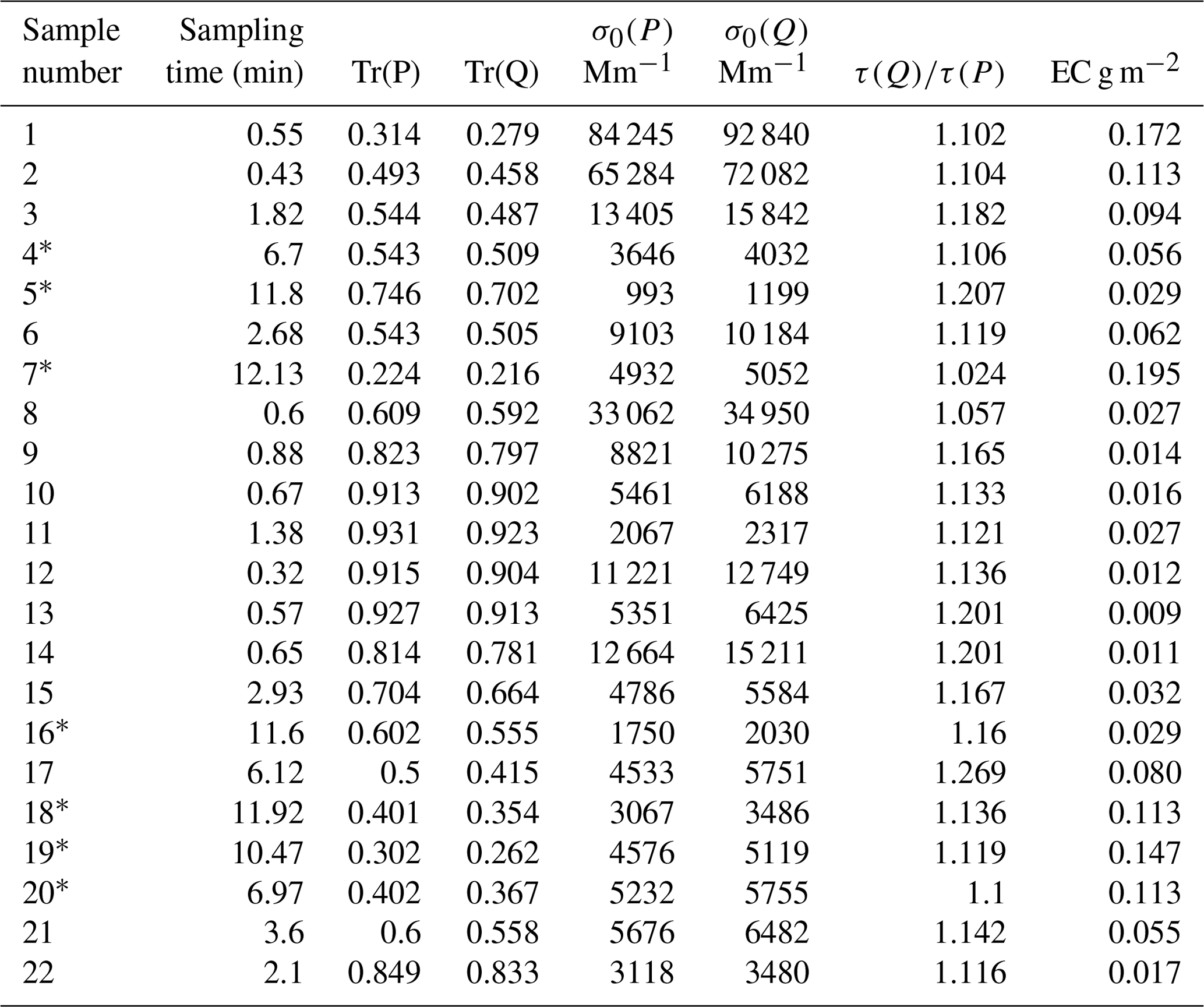
Table 1 Main information on aerosol samples taken during the experiment. Shown are sampling time, transmittances of Pallflex and quartz filters at λ=530 nm at the end of each sample (TR), attenuation coefficient, which is calculated without any loading corrections (σ₀), ratio of optical depths of quartz and Pallflex filters (τ(Q)∕τ(P)), and EC concentration in the quartz filter (EC). The 1 s data from samples denoted by ^∗ were used for deriving C_ref of quartz filters. Samples 1 and 2 were taken from the mixing chamber without any dilution.

The C_ref,P values for Pallflex E70-2075W filter were calculated here from two published calibration experiments. The loading correction function of B1999 (with the O2010 adjustment) can be reformulated as

$$\begin{array}{}\text{(7)}& f\left(\text{Tr}\right)={\displaystyle \frac{\mathrm{1}}{\mathrm{1.5557}\cdot \text{Tr}+\mathrm{1.0227}}}.\end{array}$$

This can be further rewritten as

$$\begin{array}{}\text{(8)}& f\left(\text{Tr}\right)={\displaystyle \frac{\mathrm{1}}{C_{\text{ref}}}}g\left(\text{Tr}\right)={\displaystyle \frac{\mathrm{1}}{\mathrm{2.5784}}}{\displaystyle \frac{\mathrm{1}}{\mathrm{0.6034}\cdot \text{Tr}+\mathrm{0.3966}}},\end{array}$$

where C_ref=2.5784. Similarly, the V2010 loading correction can be rewritten as

$$\begin{array}{}\text{(9)}& \begin{array}{rl}f\left(\text{Tr}\right)& =\left(k_{\mathrm{0}}+k_{\mathrm{1}}(h_{\mathrm{0}}+h_{\mathrm{1}}{\mathit{\omega }}_{\mathrm{0}})\ln \left(\text{Tr}\right)\right)\\ & =k_{\mathrm{0}}\left(\mathrm{1}+{\displaystyle \frac{k_{\mathrm{1}}}{k_{\mathrm{0}}}}(h_{\mathrm{0}}+h_{\mathrm{1}}{\mathit{\omega }}_{\mathrm{0}})\ln \left(\text{Tr}\right)\right)\\ & ={\displaystyle \frac{\mathrm{1}}{C_{\text{ref}}}}g\left(\text{Tr}\right)={\displaystyle \frac{\mathrm{1}}{C_{\text{ref}}}}\left(\mathrm{1}+{\displaystyle \frac{k_{\mathrm{1}}}{k_{\mathrm{0}}}}(h_{\mathrm{0}}+h_{\mathrm{1}}{\mathit{\omega }}_{\mathrm{0}})\ln \left(\text{Tr}\right)\right),\end{array}\end{array}$$

where h₀, h₁, k₀, and k₁ are the constants presented in Table 1 in V2010 and the single-scattering albedo ${\mathit{\omega }}_{\mathrm{o}}={\mathit{\sigma }}_{\mathrm{sp}}/({\mathit{\sigma }}_{\mathrm{sp}}+{\mathit{\sigma }}_{\mathrm{ap}})$. For the three wavelengths Eq. (10) becomes

$$\begin{array}{}\text{(10)}& {\displaystyle }& {\displaystyle }{f}_{\mathrm{467}}\left({\text{Tr}}_{\mathrm{467}}\right)={\displaystyle \frac{\mathrm{1}}{\mathrm{2.653}}}\left(\mathrm{1}-\mathrm{1.698}(\mathrm{1.16}-\mathrm{0.63}\cdot {\mathit{\omega }}_{\mathrm{0}})\ln \left({\text{Tr}}_b\right)\right),\text{(11)}& {\displaystyle }& {\displaystyle }{f}_{\mathrm{530}}\left({\text{Tr}}_{\mathrm{530}}\right)={\displaystyle \frac{\mathrm{1}}{\mathrm{2.793}}}\left(\mathrm{1}-\mathrm{1.788}(\mathrm{1.17}-\mathrm{0.71}\cdot {\mathit{\omega }}_{\mathrm{0}})\ln \left({\text{Tr}}_g\right)\right),\text{(12)}& {\displaystyle }& {\displaystyle }{f}_{\mathrm{660}}\left({\text{Tr}}_{\mathrm{660}}\right)={\displaystyle \frac{\mathrm{1}}{\mathrm{2.841}}}\left(\mathrm{1}-\mathrm{1.915}(\mathrm{1.14}-\mathrm{0.72}\cdot {\mathit{\omega }}_{\mathrm{0}})\ln \left({\text{Tr}}_r\right)\right),\end{array}$$

with $C_{\text{ref},\mathrm{467}}=\mathrm{2.653}$, $C_{\text{ref},\mathrm{530}}=\mathrm{2.793}$, and $C_{\text{ref},\mathrm{660}}=\mathrm{2.841}$.

When C_ref has been determined, it is assumed that g(Tr) is the same for both filter materials.

2.3.3 Calculation of mass absorption coefficient (MAC)

If m_EC is the mass of EC in the filter (corresponding to the spot area) through which the air volume of V_t flowed, the average mass concentration of EC in aerosol in the air volume is $c_{\text{EC,aerosol}}=m_{\text{EC}}/V_t$. If σ_ap is the absorption coefficient calculated from Eq. (4), the MAC can be calculated from

$$\begin{array}{}\text{(13)}& \begin{array}{rl}{\displaystyle }\text{MAC}& {\displaystyle }={\displaystyle \frac{{\mathit{\sigma }}_{\mathrm{ap}}}{c_{\text{EC,aerosol}}}}\\ {\displaystyle }& {\displaystyle }={\displaystyle \frac{\frac{\mathrm{1}}{C_{\text{ref}}}g\left({\text{Tr}}_t\right)\frac{A}{V_t}\mathit{\tau }}{\frac{m_{\text{EC}}}{V_t}}}\\ {\displaystyle }& {\displaystyle }={\displaystyle \frac{\frac{\mathrm{1}}{C_{\text{ref}}}g\left({\text{Tr}}_t\right)A\mathit{\tau }}{m_{\text{EC}}}}\\ {\displaystyle }& {\displaystyle }={\displaystyle \frac{\frac{\mathrm{1}}{C_{\text{ref}}}g\left({\text{Tr}}_t\right)\mathit{\tau }}{\frac{m_{\text{EC}}}{A}}}={\displaystyle \frac{f\left({\text{Tr}}_t\right)\mathit{\tau }}{m_{\text{EC}}/A}}.\end{array}\end{array}$$

This applies for aerosol but also for the snow samples, since the analysis of EC mass in a filter yields the mass surface density m_EC∕A, where m_EC is the mass of EC in the analyzed filter spot with the area A. In Svensson et al. (2018) we calculated apparent MAC values of EC in snow samples simply from $\text{MAC}=\mathit{\tau }/(m_{\text{EC}}$) without applying additional corrections for filter loading, which neither enhanced absorption by the filter medium nor light-scattering particles. Assuming that only loading and filter effects apply in the experiments presented here, the apparent MAC values presented were adjusted by using $f(\text{Tr},Q)=g\left(\text{Tr}\right)/C_{\text{ref},Q}$.

3 Results and discussion

3.1 Airborne aerosol experiment

Through our 22 airborne aerosol samples, we aimed at getting a range of transmittances and EC concentrations in the filters for the regression analysis. The original goal was to control the final transmittances by the length of the sampling time; however, this was not always successful (as noted in Table 1). Without dilution the aerosol concentration in the mixing chamber was very high, with attenuation coefficients σ₀ in the range of ∼60 000 to ∼90 000 Mm⁻¹ (see samples 1 and 2; Table 1). Therefore we added a dilution valve (V1) and a high-efficiency particulate air (HEPA) filter (Fig. 1) after the first couple of experiment runs and had variations in the ratio of sample air to clean filtered air, which led to lower σ₀ in the range of ∼1000 to ∼30 000 Mm⁻¹. The system was not always stable, resulting in different measured concentrations for similar sampling times.

3.1.1 Particle size distribution

The average size distribution measured with the Grimm 1.108 OPC shows that most particles larger than 1 µm (Fig. 2a) were efficiently removed from the air stream with the pre-separator (Fig. 1). This is uncertain, however, since the OPC was calibrated with white PSL spheres (as discussed in Sect. 2.2.3). Another important point is that the lower limit of the sizes the OPC measured was 300 nm and is probably even higher due to the above-mentioned calibration error. The particle number size distribution, nevertheless, suggests that there were large numbers of BC particles smaller than can be detected by the OPC, since the particle number concentration increases sharply with decreasing particle diameter (Fig. 2a).

The mass absorption and scattering coefficients, MAC and MSC, respectively, and single-scattering albedo ω_o of single BC particles at λ=530 nm were modeled with the Mie code of Barber and Hill (1990) and the complex refractive index of 1.85–0.71i and a particle density of 1.7 g cm⁻³. Comparison of single-particle ω_o size distribution (Fig. 2b) with the particle number size distribution (Fig. 2a) suggests that ω_o varied in the range of ∼0.3–0.5. Modeling for the size distribution measured with the OPC yielded ω_o≈0.51 and 0.54 when using the original OPC diameters and the diameters multiplied by 2, respectively. These ω_o values can be considered to be upper estimates, considering that a large fraction of small particles were undetected. However, to take the ω_o uncertainty into account, we calculated all V2010-related values by using four ω_o values: 0.3, 0.4, 0.5, and 0.6.

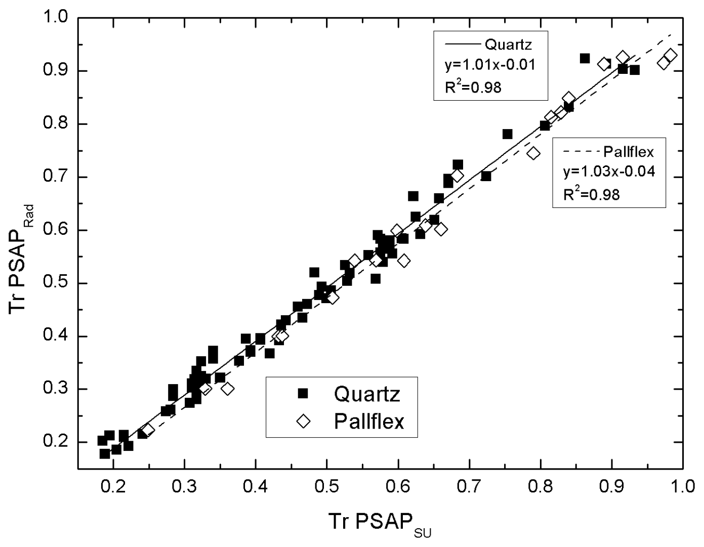
Figure 3 Transmittance for quartz and Pallflex filters measured with PSAP Radiance Research and the Stockholm University custom-built PSAP.

3.1.2 Comparison between custom built and commercial PSAPs

The optical depths presented in Svensson et al. (2018) were measured with the custom-made PSAP of Stockholm University at λ=526 nm, which is slightly different than the commercial Radiance Research PSAP (λ = 530 nm). Therefore, before applying the corrections (determined in Sect. 3.1.3 below), we examined whether the transmittances measured with these two PSAPs agree. Transmittances of all Pallflex and quartz filters were measured with both instruments. The resulting scatter plot (Fig. 3) shows that the agreement is excellent between the PSAPs; thus we concluded that the corrections established in this paper could be applied to the results presented by Svensson et al. (2018).

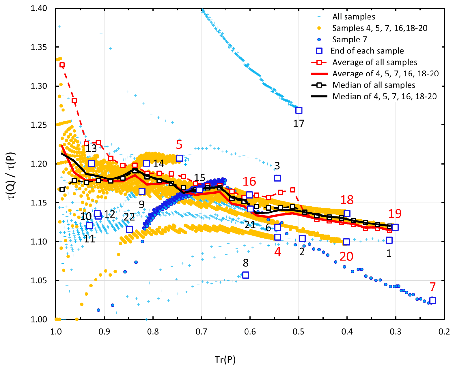
Figure 4 Ratio of non-loading-corrected optical depths ($\mathit{\tau }=\ln (\mathrm{1}/\text{Tr}))$ of quartz and Pallflex filters, τ(Q) and τ(P), respectively, at λ=530 nm at 1 s time resolution. The numbers denote the value at the end of each sample. The red numbers are associated with the samples that were used for deriving C_ref(quartz) in Sect. 3.1.2

3.1.3 Estimation of the multiple-scattering correction factor C_ref for the quartz filter

Optical depths (τ) for both the Pallflex and quartz filters, τ(P) and τ(Q), respectively, were calculated from Eq. (5) at a 1 s time resolution. The τ(Q)-to-τ(P) ratios – here the τ ratio – had a wide range of values at 1 s time resolution, but most of them were $>\mathrm{1}:\mathrm{99.6}$ % of $\mathit{\tau }\left(Q\right)/\mathit{\tau }\left(P\right)>\mathrm{1}$, and the average and median ratios were 1.21 and 1.16, respectively. To study how the τ ratio depends on filter loading, the data were classified into transmittance bins of a 0.025 width in the Tr(P) range of 0.3–1.0, and the averages and medians were calculated for each bin (shown in Fig. 4). The transmittance dependence on the τ ratio of individual samples was often controversial: in some samples it decreased from the beginning, and in some samples, it increased. We do not have an explanation of this, although the high concentrations in the mixing chamber – see the attenuation coefficients σ₀ in Table 1 – are probably largely the factor behind this observation. However, for all data the average and median τ ratio depended on the filter transmittance so that for a fresh clean filter at Tr > 0.9, it was higher than for heavily loaded filters at Tr < 0.4 (Fig. 4). In addition to the 1 s data, the τ ratio at the end of each sampling period is plotted as a function of transmittance of the Pallflex filter in Fig. 4. For the end values of all samples there was no clear Tr dependence. The most important conclusion in Fig. 4 is that the τ ratio of the two filter materials depends on the filter transmittance. On average the ratio decreases with increasing loading even though the same amount of BC is collected on both filters. That suggests that the loading corrections to be applied depend on the filter material and that they do not differ just by a constant factor.

In sample runs 4, 5, 7, 16, 18, 19, and 20, the decrease in Tr was relatively slow, and we considered the bin averages and medians calculated from them to be the most suitable to be used for determining C_ref. Sample 17 was also long, taking more than 6 min. Despite the similar settings used for filling the mixing chamber and the diluter, the τ ratio was completely different from the rest of the samples (Fig. 4). This outlier was therefore excluded from the analysis.

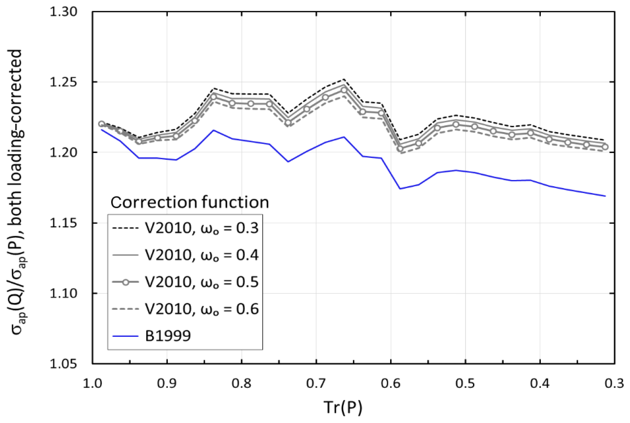
Figure 5 Average σ_ap(quartz) ∕ σ_ap(Pallflex) in 0.025 bins of transmittance of Pallflex filter at λ=530 nm. σ_ap(quartz) and σ_ap(Pallflex) were corrected either according to Bond et al. (1999) with the Ogren (2010) modification (O2010) or to Virkkula (2010; V2010) using four values for the single-scattering albedo ω_o.

The two correction algorithms (B1999 and V2010) were next applied to both filter materials, and σ_ap(Q) and σ_ap(P) (at λ=530 nm) were calculated from Eq. (4) by using the Tr bin averages and median of σ₀ and then the ratio of these two, σ_ap(Q)∕σ_ap(P). When the constants within the correction methods, including the C_ref, were the same for both filter materials, the ratio is close to 1.2 (Fig. 5). As mentioned previously, V2010 depends also on ω_o, and due to the fact that we are unsure of the ω_o of the aerosol, we present four lines (ω_o=0.3, ω_o=0.4, ω_o=0.5, and ω_o=0.6) in Fig. 4. The B1999 correction yields a slightly decreasing σ_ap(Q)∕σ_ap(P), suggesting that only adjusting C_ref would not be enough. The V2010 correction does not yield a clear Tr dependence on σ_ap(Q)∕σ_ap(P), although it has high σ_ap(Q)∕σ_ap(P) values in the Tr(P) range 0.6–0.85. They correspond to the local maxima of the average and median τ ratio shown in Fig. 4. Nevertheless, there are not enough data in this study to robustly test the correction algorithms. Therefore, all values are calculated with both of them. We next calculated the multiple-scattering correction factor C_ref from Eq. (7) by using the Tr(P) bin averages of σ_ap(Q)∕σ_ap(P). The averages and standard deviations over the Tr(P,530) range of 1–0.3 and for averaging of all four single scattering albedos, ω_o=0.3, ω_o=0.4, ω_o=0.5, and ω_o=0.6, are presented in Table 2. It is worth noting that C_ref≈3.4 at λ=530 nm is close with published values for another commonly used absorption photometer, the aethalometer, that uses quartz filters backed with supporting cellulose fibers. For instance, values around 3.5 were reported by Segura et al. (2014), Zanatta et al. (2016), and Backman et al. (2017).

Table 2 Multiple-scattering correction factors of quartz filters. C_ref(Q) is derived here for airborne BC particles from published Pallflex filter-loading corrections V2010 and O2010. C_refW(Q) is derived here for BC particles mixed in water and filtered through quartz filters. C_refSW(Q) is derived here for BC particles mixed in water and treated in an ultrasonic bath and filtered through quartz filters.

3.2 Comparison of τ vs. EC of soot mixed in water with airborne particles

The slopes of the optical depths (fτ) vs. EC concentrations, when applying the transmittance-dependent loading correction f(Tr,Q,V2010,ω_o=0.4), were different and depended on how the soot aerosol was deposited onto the filter (Fig. 7a and b). For the airborne aerosol, the slope is 6.4±0.2 m² g⁻¹, while the particles mixed in water (without the ultrasonic treatment) have a slope that is double (12.6±0.5 m² g⁻¹). Applying ω_o=0.5 and ω_o=0.6 loading corrections, the slopes of the airborne particles are 6.1±0.2 m² and 5.7±0.20 m² g⁻¹, respectively, while the slopes of the particles mixed in water (without the ultrasonic treatment) are 12.0±0.4 and 11.3±0.4 m² g⁻¹. The ratios for airborne to liquid particles are 0.506±0.026, 0.507±0.026, and 0.508±0.025 for the three choices of ω_o in the calculation. The difference in slope between the airborne and liquid particles is likely an effect of penetration depth of the soot particles into the filter media, with the higher slope for liquid particles reflecting a deeper penetration. Nevertheless, the ratio is called the water-mixing factor $f_{\mathrm{w}}\approx \mathrm{0.51}\pm \mathrm{0.03}$. In comparison, using f(Tr,B1999) for the airborne and the water-mixed particles, the slopes for optical depth fτ vs. EC concentration are 4.33±0.13 and 8.31±0.22 m² g⁻¹, respectively, providing a ratio of $f_{\mathrm{w}}\approx \mathrm{0.52}\pm \mathrm{0.02}$, essentially identical to that obtained from the V2010 correction.

The slope of fτ vs. EC of the 24 analyzed samples treated in the ultrasonic bath was even higher (Fig. 6a and b), reflecting a probable greater penetration depth of the particles. When f(Tr,Q,V2010) is calculated with ω_o=0.4, ω_o=0.5, and ω_o=0.6, the slopes of fτ vs. EC of the particles mixed in water with the ultrasonic treatment were 18.7±0.8, 17.8±0.8, and 16.9±0.7 m² g⁻¹, respectively. The average plus or minus uncertainty of the ratios of the slopes of airborne and water-mixed particles with the ultrasonic treatment is very stable, 0.34±0.02. If we consider this value to be a product of a factor f_s, representing the ultrasonic treatment and the factor f_w presented above, we obtain the value $f_{\mathrm{s}}\approx \mathrm{0.67}\pm \mathrm{0.04}$. When f(Tr,B1999) is used also for the water-mixed and ultrasonic-bath-treated particles, the slope of corrected optical depth fτ vs. EC concentration is 12.9±0.4 m² g⁻¹, with the corresponding $f_{\mathrm{s}}\approx \mathrm{0.65}\pm \mathrm{0.03}$.

Figure 6 The multiple-scattering correction factor C_ref for quartz and Pallflex filters in 0.025 bins of transmittance of Pallflex filter at λ=530 nm. The straight lines for C_ref of O2010 and V2010 are those shown in Eqs. (9) and (10).

The factors are used for multiplying $f(\text{Tr},Q)=g\left(\text{Tr}\right)/C_{\mathrm{ref}}\left(Q\right)$, and so another way it can be interpreted is that they affect the multiple-scattering correction

$$f_{\mathrm{s}}{f}_{\mathrm{w}}f\left(\text{Tr}\right)={\displaystyle \frac{\mathrm{1}}{\frac{\mathrm{1}}{f_{\mathrm{s}}}\frac{\mathrm{1}}{f_{\mathrm{w}}}{C}_{\text{ref}}}}g\left(\text{Tr}\right).$$

In other words, C_refSW(Q) = C_ref(Q)∕(f_wf_s) and $C_{\text{refW}}\left(Q\right)=C_{\mathrm{ref}}\left(Q\right)/f_{\mathrm{w}}$ for BC particles mixed in water and filtered through quartz filters with and without an ultrasonic bath, respectively. The values are presented in Table 2. The uncertainties of C_refW(Q) and C_refSW(Q) were calculated with a standard error propagation formula by using the standard deviations of C_refs in Table 2 and the uncertainties of f_w and f_s presented above.

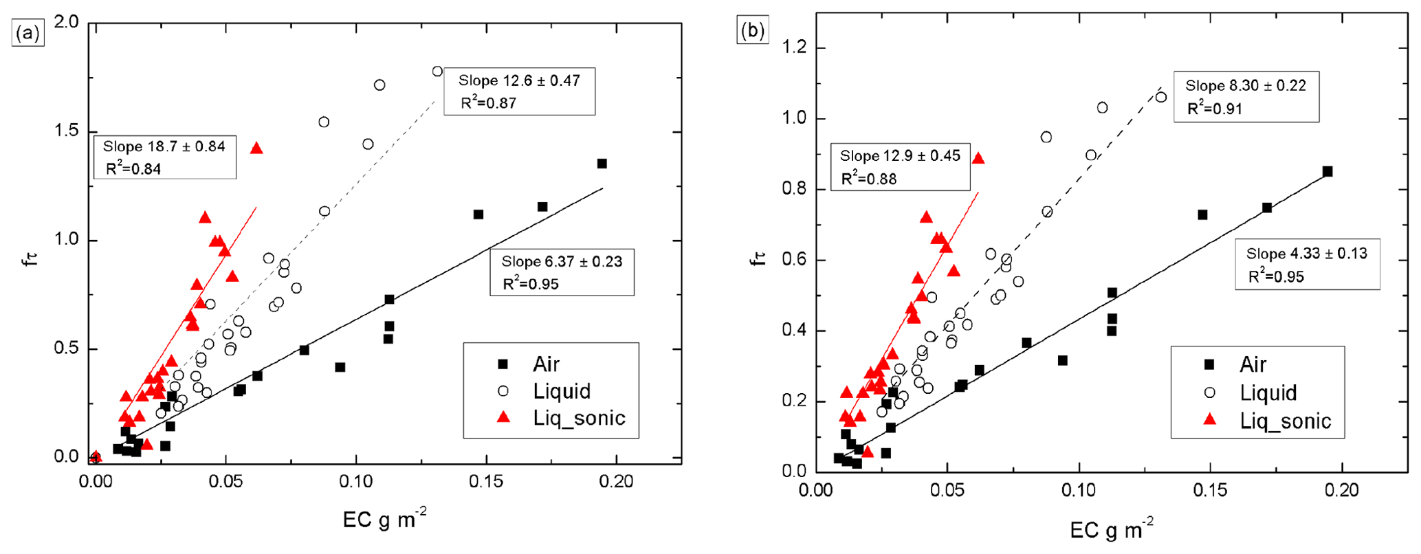
Figure 7 Linear regressions of transmittance-corrected optical depth fτ(λ=530 nm) vs. EC of the BC particles blown into the mixing chamber (Air), blown into water (Liquid), and blown into water and treated in the ultrasonic bath (Liq_sonic). The optical depths were corrected with the (a) f(Tr,V2010,ω_o=0.4) and (b) f(Tr,Q,O2010). The regressions were calculated by forcing offset to 0.

To visualize the combined effects of the loading correction functions and the two factors f_w and f_s, they are plotted as a function of τ in Fig. 8. The corresponding transmittances are shown in the secondary x axis. The range of optical depths of EC in snow presented by Svensson et al. (2018) are also shown in the figure. It is obvious that the transmittances through those filters were much lower than Tr = 0.3 used in the PSAP calibration in V2010 and even more low than the Tr = 0.6 recommended in the World Meteorological Organization and Global Atmosphere Watch (WMO/GAW, 2011) standard operating procedures. However, since there is no published calibration for such low transmittances and high optical depths for τ, the approach of extrapolating is the best method. Figure 8 also shows how V2010 and B1999 corrections are close to each other at low τ, but for dark filters at τ≈2, there is a difference of a factor of ∼2 between them.

3.3 Implications for field samples

Previously published laboratory and ambient τ vs. EC regressions in Svensson et al. (2018) were updated with the corrections developed above. Svensson et al. (2018) presented linear regressions of optical depth τ vs. EC of the same chimney soot we used in the present study, NIST soot (NIST-2975), and field samples from the Himalaya (India), and Finnish Lapland.

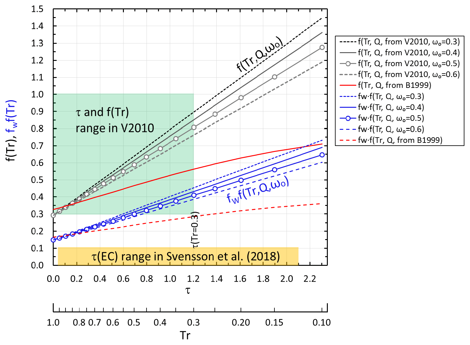
Figure 8 Loading correction functions derived from V2010 and O2010 for airborne BC particles collected on quartz filters (grey lines; f(Tr,Q,ω_o)) and for BC particles mixed in water and filtered through similar quartz filters (blue lines; f_wf(Tr,Q,ω_o)). The green shading shows the range of optical depths and f(Tr) of the V2010 Pallflex filter calibration, and the yellow shading shows the range of optical depths of EC in snow presented by Svensson et al. (2018).

We multiplied the τ of the laboratory data of Svensson et al. (2018) with f_sf_wf(Tr,V2010,${\mathit{\omega }}_{\mathrm{o}}=\mathrm{0.4},Q$), since an ultrasonic bath was also used in those experiments. The slopes of the chimney and NIST soot decreased from ∼40 and ∼35 m² g⁻¹ to 11.9±0.9 and 9.6±0.6 m² g⁻¹, respectively (Fig. 9a and b). In the scatter plot of the chimney soot, the two data points with the highest EC concentration of ∼0.04 g m⁻² are possible outliers. When they are discarded from the regression, the slope becomes 9.8±0.5 m² g⁻¹, which is indicated by the red line in Fig. 9a. This is within the uncertainties and is essentially the same as for the NIST soot.

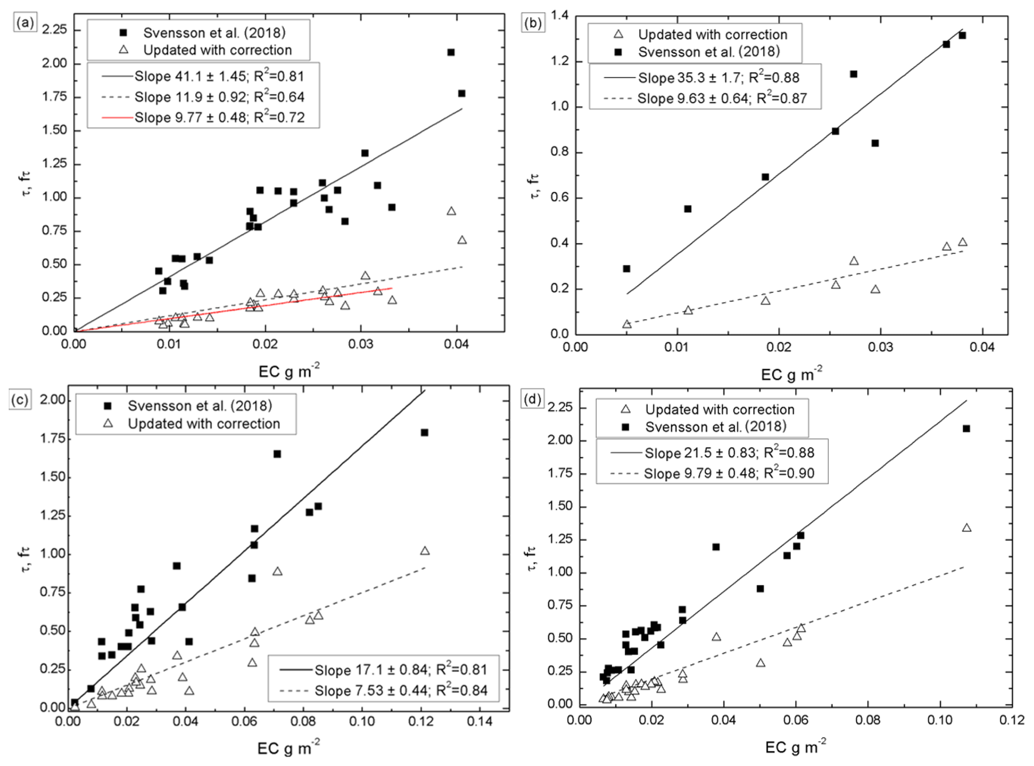
Figure 9 Reanalysis of linear regressions presented by Svensson et al. (2018). (a) chimney soot, with the red line showing the slope with the two points with the highest EC content excluded, (b) NIST soot, (c) field samples from the Indian Himalaya, and (d) field samples from Finnish Lapland. On the x axis is the EC concentration (in g m⁻²), and on the y axis are the non-corrected and corrected optical depth, τ and fτ, respectively.

These values are now of the order of published MACs, but for chimney and NIST soot, they are still considerably larger than the 6.4±0.2 m² g⁻¹ obtained in the present work (Sect. 3.2). The explanation for this difference is not clear. However, the procedures of processing the chimney soot and the NIST soot were not exactly identical to the ones we used in the present work. Svensson et al. (2018) mixed both types of soot manually in MQ water, added some ethanol to the solution, and mixed samples with variable amounts of MQ water before the ultrasonic mixing. In the present work, instead, we blew the aerosol through a virtual impactor into the MQ water, took samples of this solution, and diluted the samples before the mixing in the ultrasonic bath. The two major differences are the use of the size separation in the present work and the use of ethanol by Svensson et al. (2018), with the explanation being due to those.

For the re-evaluation of the field data presented by of Svensson et al. (2018) we multiplied the τ with f_wf(Tr,V2010,${\mathit{\omega }}_{\mathrm{o}}=\mathrm{0.4},Q$), since the field snow samples were melted and then filtered through the quartz filters. The slopes of the field samples from the Indian Himalaya and from Finnish Lapland decreased from 17.1±0.8 and 21.5±0.8 m² g⁻¹ to 7.5±0.4 and 9.8±0.5 m² g⁻¹, respectively (Fig. 9c and d). All slopes above are in the range of the published MAC of BC. For instance, Quinn and Bates (2005) obtained MAC values ranging from 6 to 20 m² g⁻¹; Bond and Bergstrom (2006) and Bond et al. (2013) reviewed several articles, and according to them the MAC of freshly generated BC is approximately 7.5±1.2 m² g⁻¹ at λ=550 nm.

4 Conclusions

Through the airborne laboratory experiments conducted in this study we determined that the multiple-scattering effect is enhanced by about 20 % with micro-quartz filters compared to Pallflex filters. In terms of the multiple-scattering correction factor, C_ref, of the quartz filters, we estimate it to be ∼3.4 for airborne sampled BC. It is worth noting that this is within the range of C_ref values published for the aethalometer, a very commonly used absorption photometer. The results of the airborne experiments also have other implications. Atmospheric aerosol is often collected on quartz filters and analyzed for EC concentration. The same filter samples can also be used for measuring light absorption to derive the MAC. The analysis showed that if this is done, the multiple-scattering correction and loading correction should be taken into account, just as they are in the data processing of online aerosol absorption photometers.

Mixing BC particles in water and filtering the solution essentially doubled the attenuation of light compared to airborne generated filters. This is probably explained by the fact that in the liquid phase and the subsequent filtering the soot particles penetrate deeper into the filter media. Deeper in the filter substrate, it is more likely that the light absorption effects are enhanced and thus account for the measured higher optical depth. In the airborne phase the depositional process is most probably different, with the particulates accumulating in the surface layer of the filter.

When samples were mixed in an ultrasonic bath before filtering through quartz filters the attenuation was further enhanced. The hypothesis for explaining the effect of the ultrasonic bath is that it possibly breaks the chain-like structure of BC particles, resulting in smaller BC particles that are able to move to further depths in the filter matrix. This remains to be confirmed and can possibly be done with electron microscopy. More research on the sampling of BC from melted snow and ice onto filter media is much needed.

All these effects mean that the absorption data obtained from melted snow samples have high uncertainties. However, the application of the correction functions to earlier published field data from the Himalaya and Finnish Lapland yielded MAC values of ∼7–10 m² g⁻¹ at λ=550 nm, which is in the range of the published MAC of airborne BC aerosol. This gives indirect support for the validity of the PSAP calibration also for darker filters than those used as the limit in atmospheric measurements.