Measurements and quality control of ammonia eddy covariance fluxes: a new strategy for high-frequency attenuation correction

Measurements of the surface–atmosphere exchange of ammonia (NH₃) are necessary to study the emission and deposition processes of NH₃ from managed and natural ecosystems. The eddy covariance technique, which is the most direct method for trace gas exchange measurements at the ecosystem level, requires trace gas detection at a fast sample frequency and high precision. In the past, the major limitation for measuring NH₃ eddy covariance fluxes has been the slow time response of NH₃ measurements due to NH₃ adsorption on instrument surfaces. While high-frequency attenuation correction methods are used, large uncertainties in these corrections still exist, which are mainly due to the lack of understanding of the processes that govern the time response. We measured NH₃ fluxes over a corn crop field using a quantum cascade laser spectrometer (QCL) that enables measurements of NH₃ at a 10 Hz measurement frequency. The 5-month measurement period covered a large range of environmental conditions that included both periods of NH₃ emission and deposition and allowed us to investigate the time response controlling parameters under field conditions. Without high-frequency loss correction, the median daytime NH₃ flux was 8.59 ng m⁻² s⁻¹ during emission and −19.87 ng m⁻² s⁻¹ during deposition periods, with a median daytime random flux error of 1.61 ng m⁻² s⁻¹. The overall median flux detection limit was 2.15 ng m⁻² s⁻¹, leading to only 11.6 % of valid flux data below the detection limit. From the flux attenuation analysis, we determined a median flux loss of 17 % using the ogive method. No correlations of the flux loss with environmental or analyser parameters (such as humidity or inlet ageing) were found, which was attributed to the uncertainties in the ogive method. Therefore, we propose a new method that simulates the flux loss by using the analyser time response that is determined frequently over the course of the measurement campaign. A correction that uses as a function of the horizontal wind speed and the time response is formulated which accounts for surface ageing and contamination over the course of the experiment. Using this method, the median flux loss was calculated to be 46 %, which was substantially higher than with the ogive method.

1 Introduction

Knowledge of ammonia (NH₃) exchange processes between ecosystems and the atmosphere is essential for improving our understanding of its impact on air quality, global warming and ecosystem health. As the most abundant base in the atmosphere, NH₃ is responsible for the formation of ammonium aerosol, impairing air quality and affecting climate. For example, it is estimated that 34 % of fine particulate matter in Europe is directly linked to emission of NH₃ that generates secondary particulate matter (Pozzer et al., 2017). Ammonium aerosol is often found to be the dominant particulate matter component in areas with strong ammonia sources, as was recently reported for North China and the Great Salt Lake region (Li et al., 2019; Moravek et al., 2019). Furthermore, deposition of NH₃ has been shown to strongly impact low-nitrogen ecosystems, thereby reducing biodiversity (Erisman et al., 2013).

Major sources of NH₃ to the atmosphere are emissions from agriculture, with 24 Tg yr⁻¹ from livestock and livestock waste and 9.4 Tg yr⁻¹ from synthetic fertiliser applications on agricultural fields being emitted globally (Paulot et al., 2014). In urban environments, fossil-fuel based NH₃ emissions can be the dominant source (Pan et al., 2016). The understanding and quantification of these emission sources is critical to propose effective NH₃ control and mitigation strategies. However, to date large uncertainties exist regarding the magnitude of NH₃ emissions. This is in part due to difficulties and challenges in measuring NH₃ fluxes, especially in environments where NH₃ fluxes are small and/or frequent changes between net emission and deposition are expected.

To measure NH₃ exchange at the ecosystem level, micrometeorological methods including gradient, relaxed eddy accumulation (REA) and eddy covariance (EC) have been used in the past. The method used largely depends on the expected flux magnitude, the site layout and the available instrumentation. Systems based on the capture of NH₃ by denuders or the thermal conversion to nitric oxide (NO) have been employed for flux gradient (e.g. Famulari et al., 2010; Flechard and Fowler, 1998; Sutton et al., 2000; Walker et al., 2006; Wolff et al., 2010) and REA-based flux measurements (Baum and Ham, 2009; Hansen et al., 2013, 2015; Hensen et al., 2009; Myles et al., 2007; Nelson et al., 2017; Zhu et al., 2000). The success of both methods often relies on the precise and accurate determination of a concentration difference measured over a typical time period of 30 min up to several hours. Especially under conditions where the measured vertical concentration gradient is small, like for flux measurements above forests, the REA method is the much stronger approach. The flux gradient measurement heights and the size of the REA deadband largely impact the concentration difference, and their choice has to be considered carefully in the flux measurement set-up and operation (Moravek et al., 2014).

The eddy covariance method is the most direct method of quantifying ecosystem-scale turbulent fluxes as it relies on the covariance between the near-ground turbulence and the scalar of interest. For this, the scalar has to be measured at a fast time response (≤0.1 s) with concurrent adequately high precision. In the last 2 decades, the development and improvement of mass spectrometry and infrared spectroscopy techniques for fast measurements of NH₃ provided the opportunity to measure NH₃ fluxes using eddy covariance. Shaw et al. (1998) presented the first eddy covariance measurements of NH₃ using a tandem mass spectrometer, and Sintermann et al. (2011) employed a proton transfer reaction mass spectrometer to measure NH₃ emissions after slurry application. For laser-based eddy covariance measurements, Famulari et al. (2004) and Whitehead et al. (2008) utilised diode laser absorption spectroscopy using cryogenically cooled lasers. A greater laser stability and output power is given by quantum cascade lasers (QCL) which can be Peltier-cooled (McManus et al., 2010). Ferrara et al. (2012, 2016) and Whitehead et al. (2008) used pulsed QCL spectrometers for NH₃ eddy covariance measurements on agricultural sites, whereas Zöll et al. (2016) employed a more sensitive continuous-wave QCL instrument to measure NH₃ fluxes above a peatland.

The common limitation of the previous studies using fast-response NH₃ analysers is the instrument time response due to the surface adsorption of NH₃. It is well-known that adsorption and desorption of NH₃ to and from surfaces, including inlet tubing, can be significant. This effect slows the time response of the measuring system leading to high-frequency attenuation (HFA) of the measured NH₃ time series, which affects the NH₃ flux measurements by eddy covariance. To avoid these effects, Sun et al. (2015) employed a custom-built open-path QCL (Miller et al., 2014) to measure eddy covariance fluxes above a cattle feedlot. While open-path QCL systems have the advantage of avoiding HFA effects, they may introduce flow distortion due to their size when placed close to the sonic anemometer and require frequent cleaning of the exposed cell mirrors (Sun et al., 2015). As closed-path systems will still play an important role in the future, our study focuses on the performance and quality control of closed-path eddy covariance systems. The magnitude of flux loss due to HFA in closed-path systems is highly variable depending on the instrumental set-up and meteorological conditions. For past NH₃ eddy covariance field measurements, the estimated flux loss ranged between 20 % and 50 % (Ferrara et al., 2012, 2016; Sintermann et al., 2011; Whitehead et al., 2008; Zöll et al., 2016). Although the flux loss can be corrected for in post-processing using spectral correction techniques, the applied correction factor can vary significantly depending on the chosen correction method (Ferrara et al., 2012). A lack of understanding of the factors impacting the time response of NH₃ eddy covariance systems is responsible for this uncertainty.

From previous studies, it is known that adsorption and desorption of NH₃ is governed by the surface area and material of the inlets and internal instrument components, with stainless steel showing significantly slower time responses than polyethylene (PE) or polytetrafluoroethylene (PTFE) (Whitehead et al., 2008). Ellis et al. (2010) showed that heating of their perfluoroalkoxy (PFA) inlet tubing to 40 ^∘C for NH₃ mixing ratios above 30 ppbv reduced the HFA significantly, whereas Sintermann et al. (2011) found that heating their drift tube inlet to 180 ^∘C enabled a time resolution high enough for eddy covariance measurements. It is suspected that heating removes – at least partially – liquid and molecular water layers on the surface, which decreases the adsorption sites for the polar NH₃ molecule (Sintermann et al., 2011), although NH₃ can also interact directly with the surface material. Roscioli et al. (2015) showed that using active passivation by continuously adding a fluorinated amine into the sample gas improved the time response significantly, as the polar amine group of the molecule occupies potential NH₃ adsorption sites and NH₃ does not react with its non-polar fluoro chain. Still, there is a lack of comprehensive mechanistic understanding of NH₃ sorption on surfaces (Sintermann et al., 2011), which is needed to reduce the uncertainties of the HFA correction for NH₃ eddy covariance fluxes. There is evidence that adsorption and desorption processes act at different rates (Whitehead et al., 2008), which would skew the high-frequency NH₃ distribution and may impact the flux covariance calculation. While Ellis et al. (2010) found the time response to degrade with the relative humidity of ambient air, the potential effect on NH₃ fluxes is not accounted for in the currently used HFA flux correction methods (Ferrara et al., 2012; Zöll et al., 2016). Evidence that the time response is improved when the NH₃ mixing ratio changes are larger (Ellis et al., 2010) can be interpreted in two ways: fluxes with higher magnitudes need to be corrected less than small fluxes, or fluxes at higher ambient concentrations are less attenuated due to a higher passivation of the surface. Finally, the time response effect of surface ageing and surface deposition of particulate matter is poorly understood and accounted for in HFA correction methods (Roscioli et al., 2015; Sintermann et al., 2011; Whitehead et al., 2008). As our understanding of the NH₃ time response in changing environmental and instrumental conditions is limited, the analysis of flux datasets under a wider range of conditions than previously sampled are needed reduce the uncertainties in the HFA correction of NH₃ fluxes.

In this study, we employed a NH₃ eddy covariance system over an entire growing season from May to October 2017 at a corn field in Eastern Canada. The system used a closed-path continuous wave QCL spectrometer with a 5.5 m heated PFA inlet line. The objectives were to (1) limit adsorption/desorption of NH₃ in the inlet of the QCL, and (2) quantify its impact on the systems time response under a large range of environmental and instrumental conditions in order to obtain a deeper understanding of the processes that govern the time response and of how this is ultimately applied to the NH₃ flux correction. This includes, for example, the examination of the relationship between time response and humidity or the flux magnitude. Due to the 5-month measurement period, we are able to examine the effect of inlet ageing and the benefit of cleaning procedures on the NH₃ flux measurement. Based on our findings, we present an approach to correct NH₃ fluxes that uses our improved understanding of NH₃ time response. The approach may also be used for flux correction of other species that show a strong surface adsorption, such as nitric or organic acids.

Next to the issue of HFA, NH₃ measurement systems need to resolve small NH₃ mixing ratio fluctuations at high time resolution. Especially under low flux conditions, a precise and stable operation of the NH₃ measurement system is required. For this reason, the paper also discusses the precision and flux detection limit of the QCL spectrometer depending on environmental and operational conditions. Currently, continuous wave QCL spectrometers are the most precise high time resolution NH₃ measurement systems available; however, their operation under field conditions requires careful set up and regular maintenance. With our findings we provide details on the set-up and operation of the QCL which are helpful for investigators that aim to use it for eddy covariance NH₃ flux measurements in the future.

2 Methods

2.1 Flux measurements

2.1.1 NH₃ detection with QCL

A quantum cascade tunable infrared laser differential absorption spectrometer (QC-TILDAS, Aerodyne Research Inc., USA) was used to measure the NH₃ mixing ratio at a 10 Hz sampling frequency for eddy covariance flux measurements. The QC-TILDAS (referred to as QCL hereafter) retrieves the NH₃ absorption spectrum at 967.3 cm⁻¹ using a thermoelectrically cooled continuous wave quantum cascade laser (Alpes Lasers, Switzerland), which is scanned across the full NH₃ transition within the spectral window. A continuous wave laser has an increased power output over a pulsed laser, which was used in the version of the QCL described in detail by Ellis et al. (2010), and is therefore more suitable for the high precision measurements needed for the eddy covariance method. As illustrated in Fig. 1, the laser beam is directed into an astigmatic Herriot multiple pass absorption cell (0.5 L, 76 m effective pass length) coated with a hydrophobic coating to reduce the interaction of NH₃ with cell walls. To minimise line-width broadening of the absorption peak, the pressure in the absorption cell is kept at approximately 4.67 kPa. A reference cell containing ethylene (C₂H₄), a less surface reactive gas that contains an absorption line near that of NH₃, is used for absorption line lock. The signal and reference paths are focused on the same thermoelectrically cooled mercury–cadmium–telluride (HgCdTe) infrared detector (Vigo Systems, Poland).

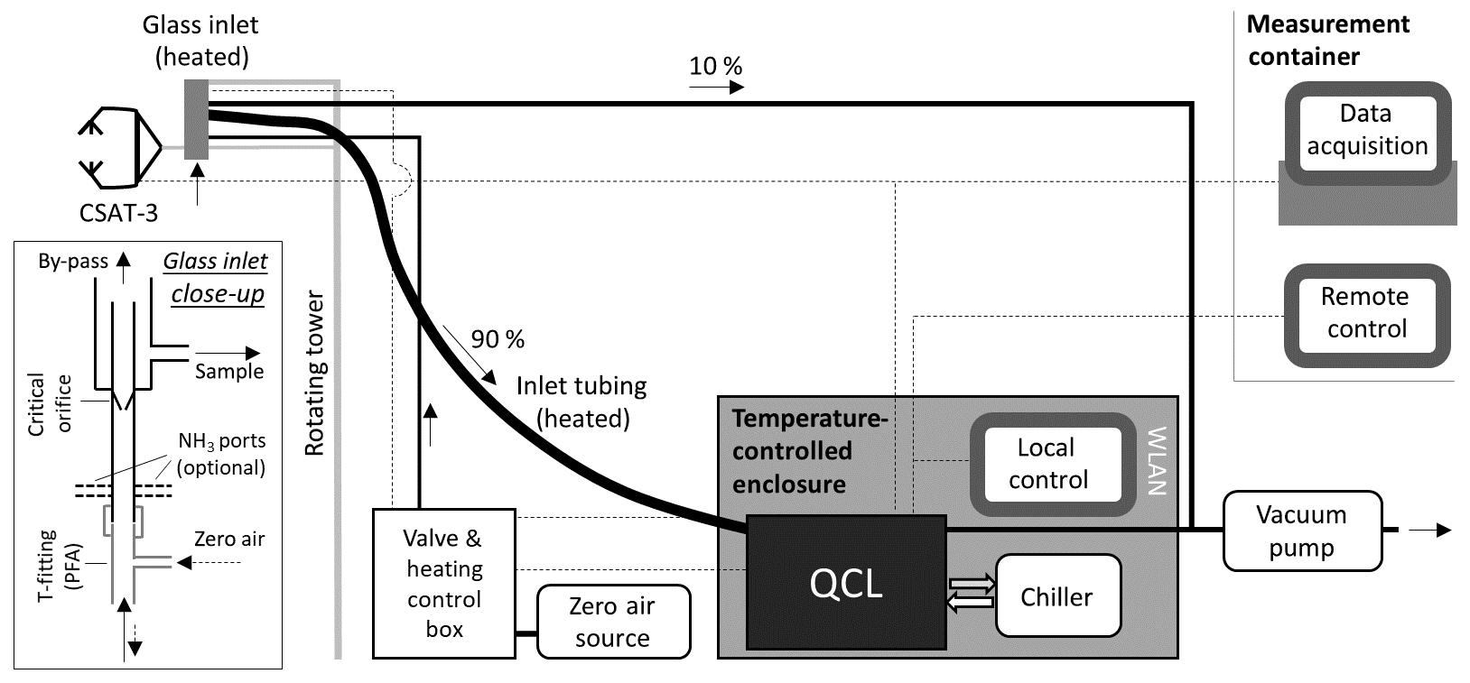
Figure 1 Schematic overview of the measurement set-up. The glass inlet of the QCL is mounted next to the sonic anemometer (measurement height 2.5 m, later 4.5 m). Inside the glass inlet (see Ellis et al., 2010), a critical orifice reduces the pressure regime and a sharp turn of the flow path leads to a reduction of particulate matter. Heated sample tubing (length of 5.5 m) leads the sample air (flow rate of 13.4 to 15.4 L min⁻¹) to the QCL, which is housed in a temperature and humidity controlled enclosure. Dotted lines show the electrical connections for data acquisition and control of the inlet heating and QCL analyser.

The laser control, spectral retrieval and mixing ratio calculations are managed by the TDLWintel software package (Aerodyne Research Inc., USA) described in Nelson et al. (2004). The measured NH₃ spectrum is fitted at the 10 Hz sample frequency by convolving the laser line shape with a calculated absorption line shape based on the HITRAN (high-resolution transmission) molecular absorption database and the measured pressure, temperature and path length of the optical cell (Herndon et al., 2007). The software allows for automatic user-defined additions of zero air via the use of a solenoid valve.

Variations in pressure, temperature and other disturbances may significantly impact the instrument performance by influencing the absorption spectrum fringe pattern. Fringes are structures in the absorption spectrum that are caused by optical interferences within the laser beam path and can be responsible for signal drift if their pattern changes over time. Especially for species that are typically present in the atmosphere in the lower parts per billion or parts per trillion mixing ratio range, such as NH₃, the impact of fringes to the absorption peak range can be significant. For that reason, the operation of the QCL requires a stable environment to house the QCL and frequent background measurements with zero air to account for potential drifts in the background spectrum.

2.1.2 Set-up and operation of NH₃ flux measurements

Eddy covariance flux measurements of NH₃ were performed from 28 May to 23 October 2017 on an agricultural corn field, equipped with twin flux towers near Ottawa in Eastern Canada (see Fig. 7, Pattey et al., 2006). The experimental site is located on the premises of the Canadian Food Inspection Agency (CFIA) and is managed by Agriculture and Agri-Food Canada (AAFC). Prior to the measurements, the agricultural field was tilled and fertilised on 25 May using granular urea fertiliser (155 kg N ha⁻¹). The corn crop was seeded on 28 May. The QCL was installed on the west eddy covariance flux tower, which had a fetch of 200 to 500 m depending on the wind direction.

To measure the 3-D wind vector for the covariance calculation, a CSAT3 (Campbell Scientific Inc, USA) sonic anemometer was installed on the tower at 2.5 m above ground level (a.g.l.). To accommodate the growing corn canopy, the tower was raised to a measurement height of 4.5 m a.g.l. on 6 July. Water vapour (H₂O) and carbon dioxide (CO₂) were measured using a closed-path infrared gas analyser (LI-7000, LI-COR, USA). The AAFC in-house data acquisition and control system, called “REAsampl” (Pattey et al., 1996), was used to record the analogue channels of the various instruments at 20 Hz. The REAsampl software adjusts the predetermined lags between the various close-path analysers and the vertical wind velocity, and rotates the horizontally symmetrical sonic anemometer head in the mean horizontal wind direction every hour when the hourly mean horizontal wind velocity is greater than 1.5 m s⁻¹. During the few seconds of the rotation for aligning the anemometer, the raw data are not recorded. By aligning the anemometer, the flow distortion and lateral loss of covariance are minimised.

As shown in Fig. 1, the set-up of the QCL consisted of five major parts: (1) the inlet system, (2) the QCL and chiller unit, (3) the valve and heating control box as well as enclosure housing, (4) the vacuum pump and (5) the zero air source. The inlet was mounted at the mid-vertical distance of the sonic anemometer open-path and 25 cm behind the anemometer open-path to minimise flow distortion from the inlet on the wind velocity measurements and lateral loss of covariance. The QCL uses a 10 cm quartz inlet which acts as virtual impactor to remove particulate matter from the sample air. As described in more detail in Ellis et al. (2010), about 90 % of the sample air makes a sharp turn (Fig. 1) and is pulled through the absorption cell, while 10 % of the flow, including particles larger than 300 nm due to their higher inertia, is pulled directly to the vacuum pump (TriScroll 600, Agilent, USA). To limit the condensation of water and the interaction of NH₃ with inlet surfaces, the glass inlet was internally coated with a hydrophobic fluorinated silane coating and was heated constantly to 40 ^∘C. The glass inlet acts as a critical orifice that regulates the volume flow at the inlet. From 28 May to 27 July a glass inlet with a flow rate of 15.4 L min⁻¹ was used, and after that period a glass inlet with a flow rate of 13.4 L min⁻¹, which had a newly applied silane coating, was utilised. For closed-path eddy covariance measurements, a high volume flow rate is essential to keep a plug flow in the inlet system, in order to minimise HFA in the inlet system. Depending on the flow rate and the actual sample gas temperature, the Reynolds number ranged between 3000 and 3700, indicating mainly transitional flow conditions with turbulent flow in the centre and laminar flow near the tubing walls. The glass inlet was connected to the QCL via a 5.5 m long $\mathrm{3}/{\mathrm{8}}^{\prime \prime }$ PFA sample tube, which was insulated and controlled to 40 ^∘C. While raising the tower on 6 July, the QCL was also raised by 2 m using wood pallets to keep a constant 5.5 m sample tube length.

The QCL, located at the bottom of the flux tower, was housed in an insulated aluminium enclosure that was equipped with two Peltier coolers to precisely control the internal temperature of the box to 28.0 (±0.2) ^∘C. Next to the QCL, the enclosure also housed the chiller (Oasis Three, Solid State Cooling Systems, USA) that was required for stable temperature control of the infrared laser and the optical and electronic parts of the QCL. To prevent the build-up of heat inside the enclosure, the intake and exhaust vents of the chiller were connected to the outside of the enclosure. A dehumidifier was built in to prevent condensation inside the box.

The time series of the 10 Hz NH₃ mixing ratios and analyser parameters were digitally recorded on the QCL computer. For precise time synchronisation between the post-processed digital NH₃ mixing ratios and the vertical wind velocity, an analogue signal of the NH₃ mixing ratio was recorded using REAsampl. A remote monitor was placed in a nearby trailer for regular checks and other operations like data transfer and manual valve switching, to avoid opening the temperature-controlled enclosure. Data were collected from the QCL computer regularly (every 2–4 d) and plotted for routine quality checks. To ensure optimal operation of the QCL instrumentation over the 5-month measurement period, the status of the QCL was checked regularly via remote access using a mobile hotspot.

Zero air for frequent background measurements was introduced at the front of the QCL glass inlet, which was designed so that zero air encountered the inlet in the same way as ambient air (Fig. 1). For zero air, a heating catalyst (Aadco Instruments, USA) was used, which scrubs NH₃ from ambient air by catalytic thermal conversion at 300 ^∘C using palladium beads. The automatic background schedule was set to flush the inlet with zero air for 5 min at the end of every 30 min period from 28 May to 16 July. Due to an operation failure of the heating catalyst, on 17 July the zero air source was replaced by ultra-high purity (UHP) compressed zero air (Praxair Canada Inc., Canada). To minimise the UHP compressed air consumption, the automated background interval was set to 1 h with a reduced duration of 3 min from 17 to 27 July. From 28 July to 31 August, the interval was set to 3 h without significantly compromising the data quality. In the final phase of the measurement period, from 15 September to 23 October, the background interval was set to 2 h. While the heating catalyst was running continuously, the zero air gas flow was introduced into the inlet by triggering a solenoid valve installed in the valve and heating control box.

To test the effect of surface ageing on the time response and to reduce the interaction of NH₃ with surfaces, regular cleaning of the glass inlet, inlet line and the absorption cell was performed by rinsing with deionised water and ethanol, while the tubing was heated to about 80 ^∘C during the cleaning process. The cleaning of the glass inlet was performed on 22 June, 27 July and 12 September. The inlet tubing was cleaned on 27 June, 27 July and 12 September. Along with cleaning of the glass inlet and the inlet tubing, the inner surface of the absorption cell was also cleaned on 12 September.

2.2 Eddy covariance flux calculation

The processing of the NH₃ data leading to the final calculated NH₃ fluxes consisted of four major steps: (1) processing and quality control (QC) of the digital NH₃ mixing ratio data, (2) time synchronisation between the quality-controlled digital NH₃ data and vertical wind velocity data recorded using REAsampl, (3) flux calculation and (4) flux random error calculation. The processing of QCL NH₃ data as well as all other processing was performed using the R software package (R Core Team, 2017).

The NH₃ mixing ratio time series were first scanned for periods of instrument failures and maintenance, which were removed. Spike detection and removal was conducted using a running-mean low-pass filter. Spikes were identified best as data points that exceeded 3.5 times the standard deviation of a 21-point averaging window. To correct for a potential drift of the QCL between two automated background periods (varying from 30 min to 3 h), the background mixing ratios were linearly interpolated between two consecutive background measurements and subtracted from the NH₃ mixing ratios. Following analogue acquisition using REAsampl, the 20 Hz CSAT3 sonic anemometer and uncorrected NH₃ data were extracted from the REAsampl raw data binary files, in which the data associated with tower rotation were already removed.

The time synchronisation between the NH₃ mixing ratios and vertical wind speed, which is essential for the eddy covariance flux calculation, was performed in two steps: (1) time synchronisation between the digital NH₃ data and the REAsampl data and (2)  time synchronisation between the digital NH₃ data and the vertical wind velocity. For the former, a circular cross-correlation was performed between the digital and analogue NH₃ signals. Accounting for the analogue output delay, the time lag between both systems was then determined as the position of the maximum correlation. In the second step, a circular cross-correlation (using a ±5 s window) between the time-synchronised sonic anemometer data and the digital NH₃ data was used to account for delays caused by the inlet system and the horizontal displacement of the CSAT3 and the glass inlet. As the cross-correlation method between the vertical wind velocity and a scalar only works well when turbulent fluxes are large enough, a quality assessment was performed on the results of the cross-correlation. Only lag times which were less than ±2.5 s and had a cross-correlation value greater than 0.05 were used. Missing lag times were then replaced by the last previous valid lag time. To detect further outliers, lag times that were offset by more than ±1.5 s were set to the preceding lag time if the difference between the preceding and successive lag time was less than 0.5 s, indicating a spike and not a real shift in the lag time. After applying the described quality control, the standard deviation of the lag time was 1.1 s, which can be partly attributed to changes in the wind speed influencing the lag time between the sonic anemometer and inlet position.

Background on the final eddy covariance flux calculation and the required correction methods is well-documented in the literature (Aubinet et al., 2012; Pattey et al., 2006). In brief, NH₃ fluxes are calculated by the covariance of the NH₃ mixing ratio (${\mathit{\chi }}_{{\mathrm{NH}}_{\mathrm{3}}}$) and the vertical wind velocity (w) multiplied by the molar density of air (ρ_m) as follows:

$$\begin{array}{}\text{(1)}& F_{{\mathrm{NH}}_{\mathrm{3}}}={\mathit{\rho }}_{\mathrm{m}}\cdot \stackrel{\mathrm{‾}}{w^{\prime }{\mathit{\chi }}_{{\mathrm{NH}}_{\mathrm{3}}}^{\prime }},\end{array}$$

where ${\mathit{\chi }}_{{\mathrm{NH}}_{\mathrm{3}}}^{\prime }$ and w^′ denote the fluctuations of NH₃ mixing ratio and the vertical wind velocity from their 30 min mean value respectively. The NH₃ fluxes presented in this study are given in nanograms of NH₃ per square metre per second (ng NH₃ m⁻² s⁻¹). Prior to the eddy covariance flux calculation, the 3-D wind vector coordinate is typically rotated to ensure zero vertical wind velocity over the averaging period (Finnigan et al., 2003; Wilczak et al., 2001). Due to the tower rotation mechanism used in this study, the wind vector was already rotated into the mean wind direction. Variations in the air density caused by temperature and air moisture fluctuations may impact the eddy covariance flux and are typically corrected for by the WPL correction (Webb et al., 1980). The sensible heat flux-induced fluctuations of the ambient air temperature are expected to be efficiently damped by the heat exchange in the inlet system and the 5 m long heated inlet line. An effect of air moisture fluctuations caused by the latent heat flux on the NH₃ flux is possible, although it was found that the effect on NH₃ fluxes is negligible (≤1 %) due to the relatively low concentrations of NH₃ in ambient air (Ferrara et al., 2016; Pattey et al., 1992). For these reasons, the WPL correction was not applied for the NH₃ fluxes in this study. High-frequency loss corrections, like for the flux loss due to the distance between the CSAT3 and the QCL glass inlet (Moore, 1986), were not applied to the initially calculated NH₃ fluxes as they were incorporated as part of the high-frequency loss analysis discussed later in this paper.

The TK3 software package (Mauder and Foken, 2011) was used to calculate fluxes of momentum, sensible heat and latent heat, and NH₃ flux quality parameters. The quality flag scheme of Foken and Wichura (1996) was used to filter for periods of low stationarity and low developed turbulence. Furthermore, the TK3 program derives the random flux errors of the NH₃ flux. The random errors include (1) the errors due to the stochastic nature of turbulence and (2) the random errors due to instrumental noise (Mauder et al., 2013). The former is calculated in TK3 following the method of Finkelstein and Sims (2001), which calculates the variance of the covariance function as a combination of the auto-covariance and cross-covariance terms with changing lag time. The random flux error due to instrumental noise is calculated in TK3 by extrapolating the auto-correlation function of the NH₃ time series towards a zero lag time (Mauder et al., 2013). As the random error calculation in TK3 was not successful for all 30 min periods, we additionally determined the instrumental noise error (${\mathit{\sigma }}_{\mathrm{cov}}^{\mathrm{noise}}$) using the variance of the zero air source measurements (conducted every 30 min to 3 h throughout the experiment) as the variance of the NH₃ mixing ratio and by implementing that in the instrumental noise function used in Mauder et al. (2013). To be comparable to other NH₃ flux studies, we also applied the approach used by Sintermann et al. (2011), where the random flux error is determined for each 30 min period by the standard deviation of the covariance function (${\mathit{\sigma }}_{\mathrm{cov}}^{\mathrm{stoch}}$) when using a time lag ranging between −120 and −70 s and +70 and +120 s. Using this approach, we defined the flux detection limit as $\mathrm{2}\cdot {\mathit{\sigma }}_{\mathrm{cov}}^{\mathrm{stoch}}$.

2.3 Time response determination of NH₃ measurements

A fast time response of the NH₃ measuring system is essential for performing eddy covariance measurements. To understand the processes that impact the adsorption and desorption of NH₃ to the measurement system, knowledge of the system's NH₃ time response is important. The time response of the QCL NH₃ measurements is mainly determined by two processes (Whitehead et al., 2008): (1) the exchange of the sample air volume in the inlet line and the sample cell and (2) the adsorption and desorption of NH₃ at the inlet and sample cell walls. As a result, the time response can be described by a double exponential function giving two time constants, τ₁ and τ₂, representing the time response towards the exchange of the sample air volume and wall interactions respectively:

$$\begin{array}{}\text{(2)}& \begin{array}{rl}f\left(t\right)& =y_{\mathrm{0}}+A_{\mathrm{1}}\cdot \exp \left({\displaystyle \frac{-(t-t_{\mathrm{0}})}{{\mathit{\tau }}_{\mathrm{1}}}}\right)\\ & +A_{\mathrm{2}}\cdot \exp \left({\displaystyle \frac{-(t-t_{\mathrm{0}})}{{\mathit{\tau }}_{\mathrm{2}}}}\right),\end{array}\end{array}$$

where t₀ is the start time and y₀ is the offset from zero (Fig. 2); A₁ and A₂ are proportionality coefficients that account for the contribution of each process to the overall time response. Accordingly, the percentage contribution of the wall interaction processes can be described as follows (Ellis et al., 2010):

$$\begin{array}{}\text{(3)}& D=\left({\displaystyle \frac{A_{\mathrm{2}}}{A_{\mathrm{1}}+A_{\mathrm{2}}}}\right)\cdot \mathrm{100}\mathit{\%}.\end{array}$$

Along with the time constants τ₁ and τ₂, D can be used to evaluate the performance of the QCL system with respect to its time response. To determine the time response for our instrument set-up, the double exponential function (Eq. 2) was fitted to the step change in the NH₃ mixing ratios when switching from ambient air to zero air measurements as part of the automated background correction. Those fits were performed for each background period in order to obtain the temporal variation of the time response over the course of the entire measurement period.

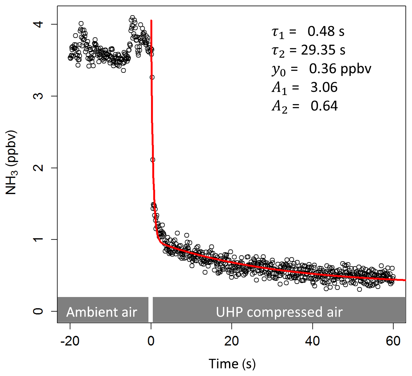
Figure 2 Time response of the 10 Hz NH₃ measurement. Shown is the step change NH₃ mixing ratios after switching from ambient air to the UHP compressed air. The red line is the fit of the double exponential decay function.

2.4 Analysis of flux loss due to high-frequency attenuation

2.4.1 Ogive method

The attenuation of the high-frequency scalar time series due to a slow response leads to an underestimation of the calculated eddy covariance flux. Both theoretical and experimental approaches are used to quantify the flux loss and ultimately correct for it; a summary is given in Foken et al. (2012). For NH₃ the HFA needs to be determined experimentally, as no adequate description of the surface adsorption and desorption processes currently exists. Experimental approaches typically compare the co-spectrum of the vertical wind velocity and the attenuated scalar time series to the co-spectrum of a non-attenuated reference flux. The sensible heat flux is most often used as a reference flux, either from direct measurements or from parameterisation available in the literature (Kaimal and Finnigan, 1994). In this study we used the ogive method described in Ammann et al. (2006). The ogive of a scalar flux (Og_ws) is calculated by the cumulative integral of the co-spectrum (Co_ws) as

$$\begin{array}{}\text{(4)}& {\mathrm{Og}}_{\mathrm{ws}}\left(f\right)={\int }_{\mathrm{1}/t}^{\mathrm{\infty }}{\mathrm{Co}}_{\mathrm{ws}}\left(f\right)\mathrm{d}f\end{array}$$

over the observed frequency range, beginning with the lowest frequency (1∕t, where t is the averaging interval). If the ogive is normalised by the covariance, the ogive value at the highest frequency is 1. The flux loss is derived by scaling the normalised ogive of the scalar flux to the normalised ogive of the sensible heat flux at a given limit frequency (f₀). The scalar ogive value at the highest frequency then represents the flux attenuation factor (between 0 and 1). The limit frequency is defined as the highest frequency at which no HFA occurs and can be determined by comparing the scalar co-spectrum to the sensible heat flux co-spectrum.

Ideally, a reference scalar is used that shows the highest scalar similarity to the investigated flux. The water vapour flux is expected to have a similar sink and source distribution to NH₃, but the measured flux may experience high-frequency loss if measured with a closed-path analyser. Therefore, in this study we used the measured non-attenuated sensible heat flux as a reference.

2.4.2 Time response method

Another approach to correct for the HFA is to simulate the flux loss by knowing the flux loss transfer function, which represents the flux attenuation factor as a function of frequency. The transfer function can be obtained by applying a low-pass filter, which represents the HFA of the system, to the time series or flux of a non-attenuated scalar and then comparing the filtered and non-filtered fluxes. In this study, we determined the transfer function through the system's time response, which was determined over the entire measurement period as described in Sect. 2.3. As for the ogive method, we used the sensible heat flux as a reference flux.

A low pass-filter can be applied either (1) in the frequency domain or (2) in the time domain. For the former method, a transfer function is applied to the sensible heat flux co-spectrum, which we modified using both τ₁ and τ₁ from Eq. (2). However, the low-pass filter effect of the inlet tubing introduces a phase shift next to the attenuation of high-frequency amplitudes (Horst, 1997; Massman and Ibrom, 2008). For that reason, we applied a low-pass filter in the time domain to the high-frequency temperature time series. This method accounts for the phase shift and was used in the past to simulate the HFA effect of eddy covariance water vapour fluxes (Ibrom et al., 2007) and of relaxed eddy accumulation systems (Moravek et al., 2013). In the time domain, a low-pass-filtered scalar time series (c_att) is retrieved as

$$\begin{array}{}\text{(5)}& c_{{\mathrm{att}}_n}=c_{\mathrm{n}}\cdot A+(\mathrm{1}-A)\cdot c_{{\mathrm{att}}_{\mathrm{n}}},\end{array}$$

where c is the non-attenuated scalar time series and A is the filter constant. For a given sampling frequency (f_s), this constant depends on the cut-off frequency (f_c), which is the frequency at which the filter reduces by a power of 2:

$$\begin{array}{}\text{(6)}& A=\mathrm{1}-e^{-\mathrm{2}\mathit{\pi }\cdot \left(f_{\mathrm{c}}/f_{\mathrm{s}}\right)},\end{array}$$

where f_c can be characterised by the time constant τ as

$$\begin{array}{}\text{(7)}& f_{\mathrm{c}}={\displaystyle \frac{\mathrm{1}}{\mathrm{2}\cdot \mathit{\pi }\cdot \mathit{\tau }}}.\end{array}$$

As the time response for NH₃ is described by two time constants, we low-pass filtered the high-frequency temperature time series using both τ₁ and τ₂, where τ₁ is the time constant describing the exchange of sample air volume and τ₂ is the time constant accounting for wall interactions. The respective low-pass-filtered time series, $c_{{\mathrm{att}}_{\mathrm{1}}}$ and $c_{{\mathrm{att}}_{\mathrm{2}}}$, can then be combined as

$$\begin{array}{}\text{(8)}& c_{\mathrm{att}}=\left(\mathrm{1}-D/\mathrm{100}\right)\cdot c_{{\mathrm{att}}_{\mathrm{1}}}+D/\mathrm{100}\cdot c_{{\mathrm{att}}_{\mathrm{2}}},\end{array}$$

using the D value from the time response analysis. The transfer function using the time domain low-pass filter method, T_time(f), is then defined as the ratio between the attenuated and non-attenuation sensible heat flux co-spectrum

$$\begin{array}{}\text{(9)}& T_{\mathrm{time}}\left(f\right)={\displaystyle \frac{{\mathrm{Co}}_{{\mathrm{wc}}_{\mathrm{att}}}\left(f\right)\mathrm{d}f}{{\mathrm{Co}}_{\mathrm{wc}}\left(f\right)\mathrm{d}f}}.\end{array}$$

To account to for the time lag introduced by the phase shift of the low-pass filter, a circular cross-correlation between the overall low-pass-filtered temperature and the vertical wind velocity time series was performed beforehand. The flux attenuation factor using the time response method (α_tr) is then determined by the ratio of the filtered co-spectrum and the non-filtered co-spectrum of the sensible heat flux, which is equal to the ratio of the attenuated and non-attenuated sensible heat flux covariance:

$$\begin{array}{}\text{(10)}& {\mathit{\alpha }}_{\mathrm{tr}}={\displaystyle \frac{{\int }_o^{\mathrm{\infty }}{\mathrm{Co}}_{w{T}_{\mathrm{att}}}\left(f\right)\mathrm{d}f}{{\int }_o^{\mathrm{\infty }}{\mathrm{Co}}_{wT}\left(f\right)\mathrm{d}f}}={\displaystyle \frac{\mathrm{cov}\langle w,c_{\mathrm{att}}\rangle }{\mathrm{cov}\langle w,c\rangle }}.\end{array}$$

To investigate the possible NH₃ flux loss over the measurement period, the flux loss was simulated for all 30 min periods, using τ₁, τ₂ and D values that represent the range of observed time responses.

3 Results

3.1 Measured NH₃ fluxes, random flux error and flux detection limit (before HFA correction)

The QCL eddy covariance measuring system was operated over a period of 149 d between May and October 2017, covering a total of 7132 flux measurement periods. Times of system maintenance, quality control checks and other system downtime were discarded from the dataset, resulting in a flux data coverage of around 85 % (Table 1).

Table 1 Statistics of the NH₃ flux quality control for the flux data collected over the 5-month experiment period. Values given in nanograms per square metre per second (ng m⁻² s⁻¹) represent the median value for the period.

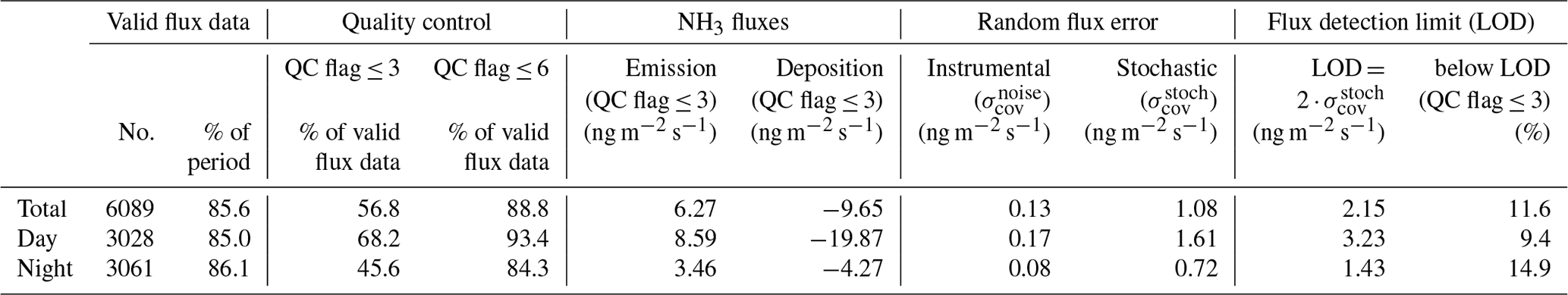
Figure 3 shows the statistics of flux magnitudes for each month from May to October before applying any HFA correction. Flux magnitudes are compared to the median diurnal flux detection limits of each month. As illustrated in the top-right corner of each month, the diurnal flux magnitudes were comprised of both NH₃ emission and deposition fluxes. Although fluxes in May only represent 4 days, the overall maximum flux of around 500 ng m⁻² s⁻¹ was observed in that period. While June and July were mainly dominated by small fluxes, typically less than ±10 ng m⁻² s⁻¹, in August clear emission was observed with a daytime median value of around 20 ng m⁻² s⁻¹. September marked an emission to deposition transition period, with significant deposition fluxes reaching as high as −300 ng m⁻² s⁻¹. In October, fluxes were dominated by deposition, with a median daytime value of around −30 ng m⁻² s⁻¹. Over the entire period, the daytime median flux was 8.6 ng m⁻² s⁻¹ during periods of emission and −19.87 ng m⁻² s⁻¹ during periods of deposition (Table 1). Night-time fluxes were significantly lower, with median values of 3.5 and −4.27 ng m⁻² s⁻¹ respectively, showing clear diurnal cycles during periods of high emission and deposition.

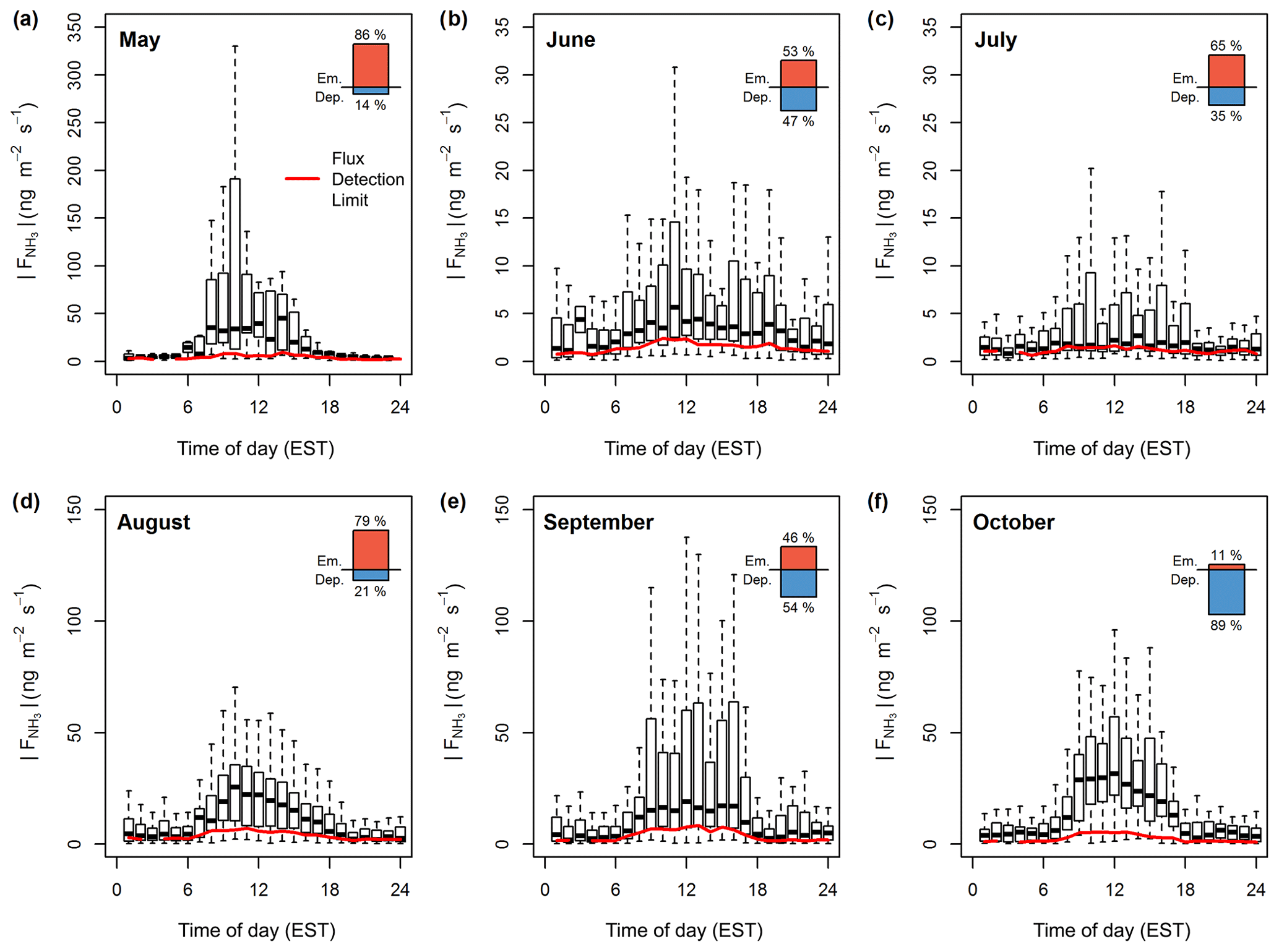
Figure 3 Box plot statistics of diurnal absolute NH₃ fluxes for each month from May to October 2017 before the application of a HFA correction. Red lines illustrate the diurnal course of the median flux detection limit. The percentages of flux periods with emission or deposition are indicated in the top-right corner of each month.

The flux statistics are affected by the choice of the flux quality flags used to remove periods of weakly developed turbulence or non-stationarity (Foken and Wichura, 1996). A quality flag ≤3 is typically used for fundamental research, whereas fluxes with quality flag ≤6 are used for long-term flux datasets. We only used fluxes with a quality flag of ≤3, leaving 68 % of daytime and 46 % of night-time fluxes (Table 1).

The random flux error due to instrumental noise (${\mathit{\sigma }}_{\mathrm{cov}}^{\mathrm{noise}}$) is dependent on the precision of the QCL and variations in the friction velocity (u_∗). Over the course of the field campaign, an average precision of 0.085 (±0.010) ppbv at the 10 Hz sample frequency was achieved, which was independent of the measured NH₃ mixing ratio. The resulting median flux error was 0.17 ng m⁻² s⁻¹ for daytime and 0.08 ng m⁻² s⁻¹ for night-time fluxes; much lower than the median observed fluxes (Table 1). In contrast, the random error derived from the lag time shift (${\mathit{\sigma }}_{\mathrm{cov}}^{\mathrm{stoch}}$) was significantly larger, with median values of 1.61 ng m⁻² s⁻¹ during daytime and 0.72 ng m⁻² s⁻¹ during night-time. However, still only 11.6 % of the total flux data were below the detection limit (2.15 ng m⁻² s⁻¹), which shows the overall good performance of the QCL eddy covariance measuring system.

3.2 High-frequency attenuation

3.2.1 Ogive method

We applied the ogive method to the co-spectra of the sensible heat and NH₃ flux. Figure 4 shows an example of the normalised co-spectra. To illustrate the effect of HFA, the co-spectra are multiplied by the frequency; HFA is indicated if the slope of the NH₃ co-spectrum in the inertial subrange (high frequency part of spectrum) is steeper than the slope of the sensible heat flux co-spectrum. While this is not clearly visible in the co-spectra (by comparing against the expected $-\mathrm{4}/\mathrm{3}$ slope line in the inertial subrange), the ogives show a clear underestimation of the NH₃ flux at higher frequencies, illustrated by the flattened NH₃ ogive curve at high frequencies. Applying the ogive method to all 30 min periods yields a frequency distribution of the attenuation factor (Fig. 5). As the ogives may show significant noise or fluctuations, the choice of the limit frequency for the determination of the scaling factor is critical. For that reason three limit frequencies of 0.050 Hz, 0.067 and 0.100 Hz were chosen representing timescales of 20, 15 and 10 s respectively. Only periods were used where the standard deviation of the scaling factors determined at those three limit frequencies was smaller than 5 %. Furthermore, only data periods were used where both the NH₃ and sensible heat flux were significant and of sufficient data quality (TK3 flag ≤3). After applying that filter, the median flux attenuation factor was calculated to be 0.83, corresponding to a flux loss of 17 %. The spread of the observed factors was significant with 50 % of the values lying between 0.75 and 0.91; the standard deviation was 16 %. Also, for some periods the attenuation factor was above 1, which was most likely caused by uncertainties in the ogive method.

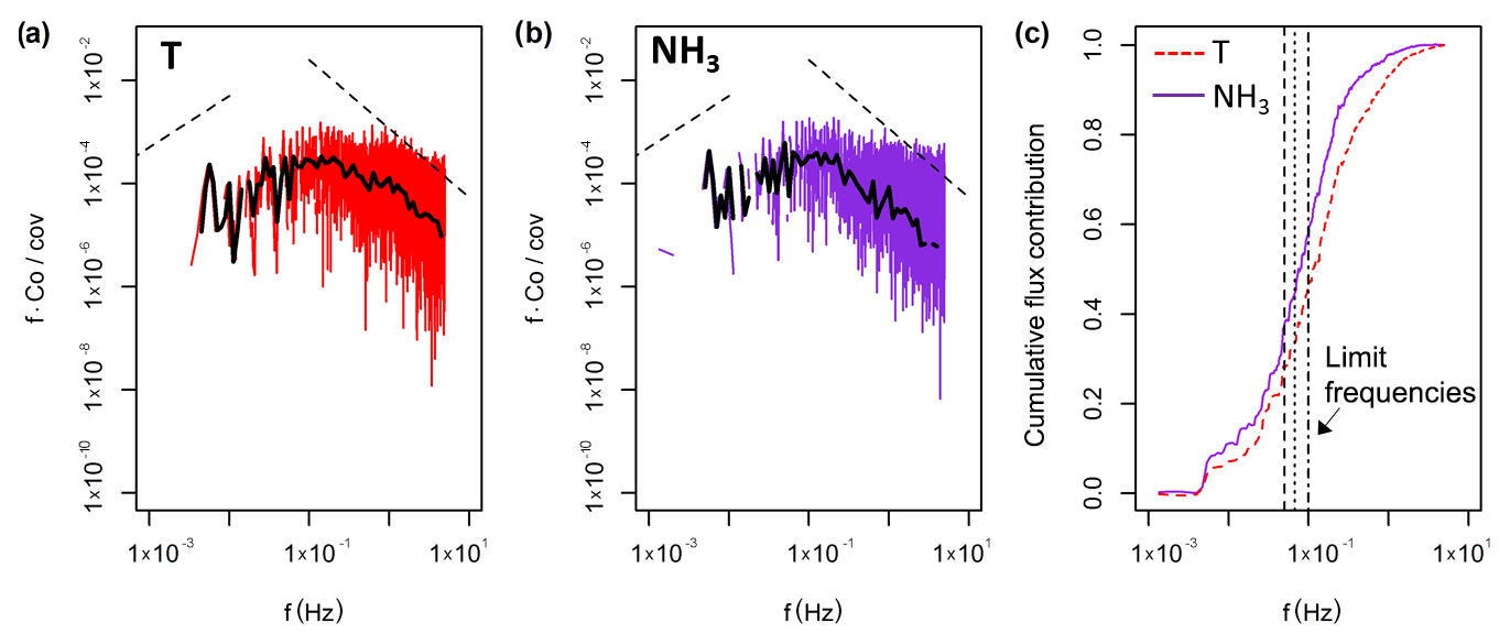
Figure 4 Results from the spectral analysis. Panels (a) and (b) show the respective co-spectral densities for the sensible heat and NH₃ flux for the period from 12:00 to 12:30 EST on 9 August 2017. The dashed lines indicate the expected slopes in the low frequency range and the inertial subrange. (c) The cumulative flux contribution (ogive) for both the sensible heat flux (T) and the NH₃ flux are shown for the same 30 min period. The dashed, dotted and dash-dotted vertical lines represent the limit frequencies used in the flux loss analysis at 0.050, 0.067 and 0.100 Hz respectively.

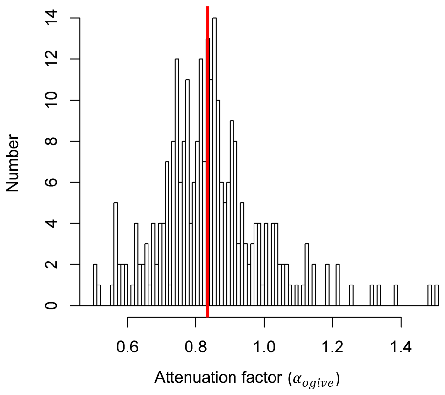
Figure 5 Results from the ogive analysis show the frequency distribution of the flux attenuation factor (α_ogive). Values lower than unity represent an underestimation of the NH₃ flux. The red vertical line marks the median value of 0.83, corresponding to a flux loss of 17 %.

To give insights into the causes of the NH₃ flux loss, the attenuation factor was analysed for dependencies on different parameters. No clear change of attenuation factor was observed over time, which would have suggested an effect of surface ageing or cleaning. Due to the uncertainties in the ogive method, the noise in the attenuation factors was larger than the effect of surface ageing or cleaning. Also, no correlation of the attenuation factor with ambient air humidity was found. The highest variation of attenuation factors occurred at conditions of neutral atmospheric stability, an indication of the limitations of the ogive method during these conditions. However, a slight decrease in the attenuation factor with increasing horizontal wind speed (u) was found (Figs. 6, S1), which is expected due to the shift of the turbulence spectra to higher frequencies with increasing wind speed. Given the non-Gaussian distribution of attenuation factors at some wind speeds, we used a quantile linear regression to obtain a function of the flux attenuation factor using the ogive method (α_ogive) with u (in m s⁻¹):

$$\begin{array}{}\text{(11)}& {\mathit{\alpha }}_{\mathrm{ogive}}=f\left(u\right)=-\mathrm{0.031}\cdot u+\mathrm{0.94}.\end{array}$$

As the majority of data used is clustered between wind speeds of 0.5 and 2.5 m s⁻¹, the correlation with wind speed is only weak as illustrated by a R² value of 0.04 of the least squares linear regression. The correlation might be impacted by changes of the aerodynamic measurement height, due to tower raise and the growth of the corn canopy over the season. However, as no clear correlation of the attenuation factor with time was found, this effect is not accounted for in the presented relation with horizontal wind speed.

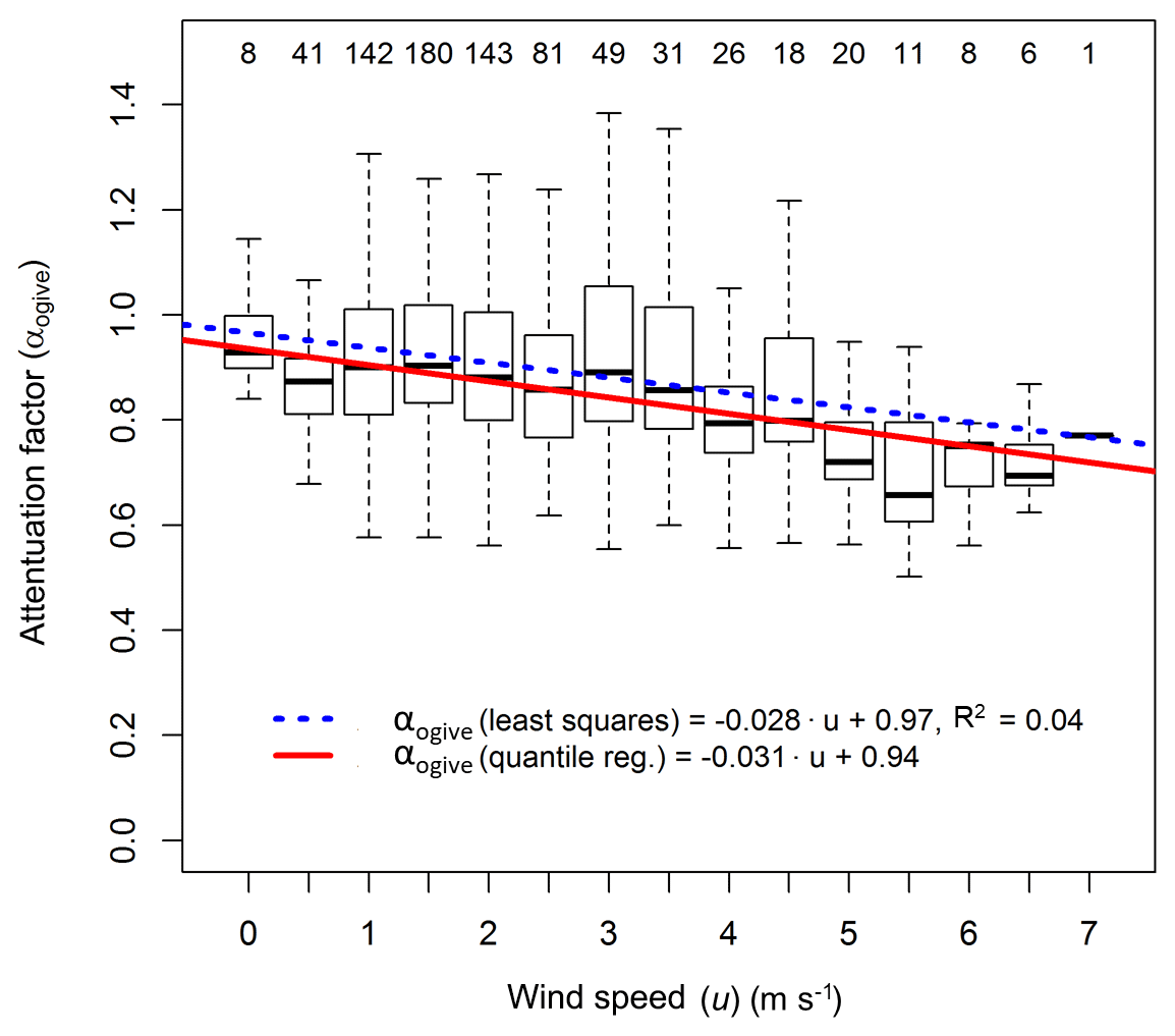
Figure 6 Box plot statistics of flux attenuation factors from the ogive analysis against the binned horizontal wind speed. Numbers on the top denote the number of data points in each bin. Both the least square and the quartile regression lines are shown. The coefficients from the quartile regression were used in Eq. (9).

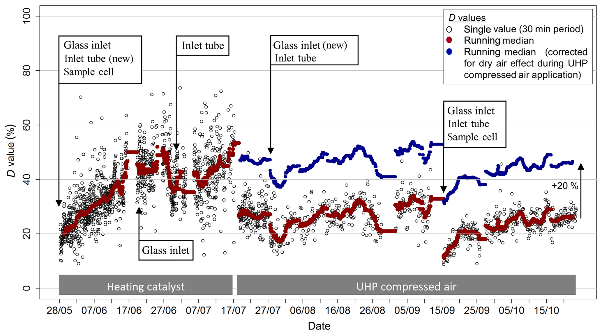
Figure 7 Variation in the time response during the experiment, represented by the D value, as well as times of cleaning of the QCL inlet system. The D value gives the percentage contribution of time constants associated with wall interactions. Red data points represent the 48 h moving median D value. To correct for the effect of dry air on the times response, the D values during times when the UHP compressed air was operated were increased by 20 % (blue data points).

3.2.2 Time response

The double exponential function used to determine the system's time response is characterised by τ₁, τ₂ and the D value. The median value for τ₁ was 0.6 s. This value is slightly higher than the calculated time constant for the exchange of air volume in the 0.5 L absorption cell (∼0.1 s). The time response needed to exchange the air volume in the inlet tubing is significantly less (< 0.03 s), due to its small volume and low pressure (< 15 kPa) in the inlet tubing. The time constant τ₂, representing the timescale for NH₃ surface interactions, showed a median value of 27 s. Both τ₁ and τ₂ did not exhibit a clear trend over time, nor a correlation with humidity or other parameters. In contrast, the D value revealed distinct differences over time. Figure 7 shows the evolution of the D value over the course of the field campaign as well as times of inlet, tube and cell cleaning. Initially, D values were around 20 % and then increased steadily to more than 50 % at the end of June. While cleaning of the glass inlet and the inlet tube in June did not directly lead to a decrease in the D value, the cleaning of the glass inlet and inlet tubing on 27 July led to a visible decrease in the D value. On 12 September, when the inlet, tubing and the surface of the absorption cell was cleaned, the largest decrease in the D values after cleaning down to 10 % was observed. Additionally, a significant overall decrease in D values was observed following 17 July , after switching the zero air source from the heating catalyst to the UHP compressed air. As the heating catalyst scrubs NH₃ from ambient air, the moisture level of the heating catalyst zero air is more similar to ambient air than to that of the dry UHP compressed air. Thus, the D value differences for the two zero air sources might be caused by different moisture levels. However, no distinct correlation of the D value with ambient air humidity was found for the heating catalyst period. A decrease in D values with increasing ambient air NH₃ mixing ratios, as discussed in Ellis et al. (2010), was detected (Fig. 8), suggesting a larger relative importance of adsorption and desorption processes at lower NH₃ mixing ratios. The increase in D values at lower NH₃ mixing ratios may also be due to the variation of D values caused by a larger uncertainty of the double exponential fit with small mixing ratio changes. While the relative random errors of A₁ and A₂ from double exponential fit increase exponentially with decreasing NH₃ mixing ratios, the propagated random error of D was typically below 10 % for NH₃ mixing ratios above 0.5 ppbv. For lower mixing ratios, only D values with a relative error of less than 50 % were used.

3.2.3 Time response method

To investigate the effect of the measured time response on the NH₃ fluxes, the flux loss was simulated using the time response method. As the time constants τ₁ and τ₂ did not show distinct trends over time like the D value, they were fixed at 0.6 and 27.0 s respectively. The flux loss was simulated for D values of 0 %, 20 %, 40 % and 60 %, which represent the observed range of D. Figure 9 shows T_time(f) for the four scenarios and their effect on the ogives of sensible heat flux for a selected 30 min period. To illustrate the contributions of the two time constants τ₁ and τ₂ as well as the influence of the phase shift, the respective frequency domain transfer functions $T_{f_{\mathrm{1}}}\left(f\right)$ and $T_{f_{\mathrm{2}}}\left(f\right)$ are shown. As the frequency domain transfer functions used here only account for the attenuation of the signal amplitudes and not the phase shift, their sum (T_f(f)) underestimates the flux loss compared with the time domain low-pass filter approach used in this study. For the 30 min period shown here, the flux loss ranged from 21 % to 64 %, increasing with higher D values, representing a higher contribution from the slow time constant that reflects adsorption/desorption. Applying the simulation for flux data from the entire measurement period, a clear decrease in the flux attenuation factor with increasing horizontal wind speed was observed (Fig. 10), which is explained by a shift of the co-spectrum to higher frequencies with increasing wind speeds. The linear regression lines for each simulation scenario are displayed in Fig. 10 including the respective linear regression functions. By expressing the slope (m) and the intercept (c) as a function of D through linear regression ($f_{m,c}\left(D\right)=m_{m,c}\cdot D+c_{m,c}$), we can describe the flux attenuation factor using the time response method (α_tr) as a single function of u and the D value as

$$\begin{array}{}\text{(12)}& \begin{array}{rl}{\mathit{\alpha }}_{\mathrm{tr}}& =f(u,D)=\left(m_m\cdot D/\mathrm{100}+c_m\right)\cdot u\\ & +m_c\cdot D/\mathrm{100}+c_c.\end{array}\end{array}$$

For the dataset presented, the linear regression yielded m_m=0.036, $c_m=-\mathrm{0.047}$, $m_c=-\mathrm{0.83}$ and c_c=0.93. The overlap of the regression lines of this generalised function with all individual regression lines in Fig. 10 shows the strong linear correlation of the flux attenuation factor with both u and the D value. In the case of D=0, Eq. (12) represents the damping that is not due to the wall interactions and would also be applicable to other, non-sticky, trace gases. After deriving α_tr, the NH₃ fluxes are then corrected individually for every 30 min period by dividing by α_tr.

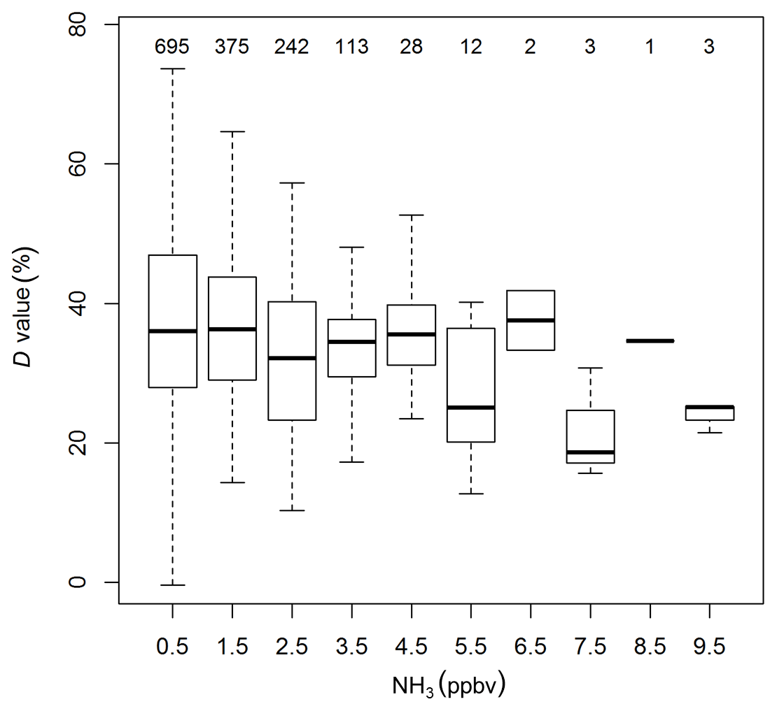
Figure 8 Box plots of statistics of time response results: D values against the binned ambient NH₃ mixing ratios before switching to the zero air source. Numbers on the top denote the number of data points in each bin.

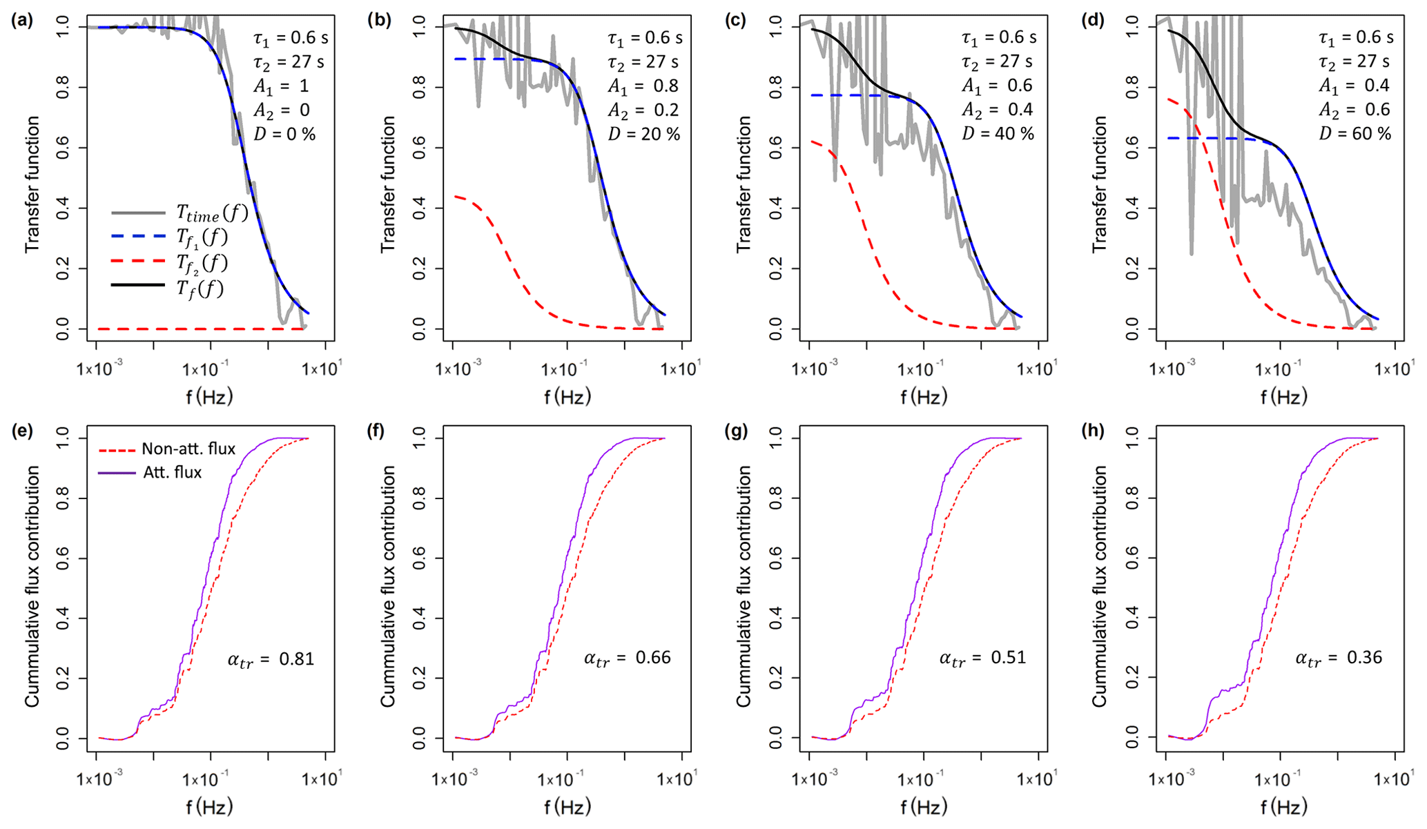
Figure 9 Results from the high-frequency loss simulation shown for the period from 12:00 to 12:30 EST on 9 August 2017. (a–d) Calculated transfer functions for four different scenarios of D (= 0 %, 20 %, 40 % and 60 %) values from the time response fitting procedure. Shown are the transfer function used in this study, T_time(f), where the high-frequency time series was low-pass filtered in the time domain, and the frequency domain transfer functions, $T_{f_{\mathrm{1}}}\left(f\right)$ and $T_{f_{\mathrm{2}}}\left(f\right)$, which illustrate the flux loss associated with τ₁ and τ₂ respectively. As the frequency domain transfer functions used here only account for the attenuation of the signal amplitudes and not the phase shift, their sum, T_f(f), underestimates the flux loss compared with the time domain low-pass filter approach used in this study. (e–f) The cumulative flux contribution (ogive) for the non-attenuated and attenuated sensible heat flux and calculated flux attenuation factors (α_tr). For each scenario the respective transfer function T_time(f) in the panel above was used.

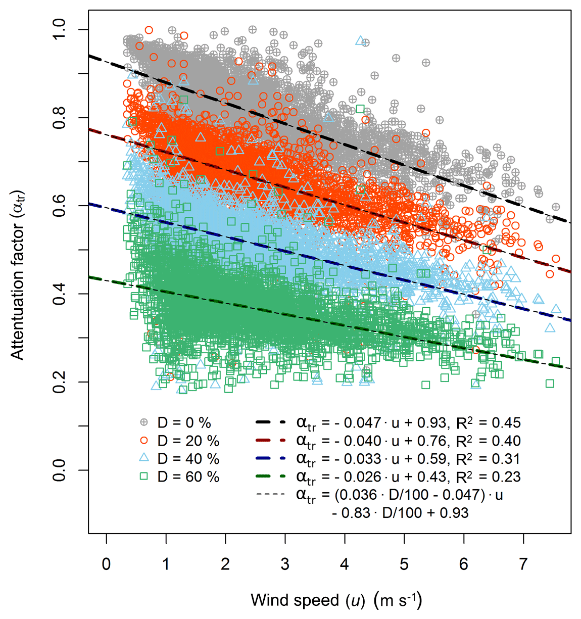
Figure 10 Correlation of the flux attenuation with horizontal wind speed for the different low-pass filter scenarios. The simulation was performed for all 30 min periods of the experiment, while for each scenario a linear regression function was derived. The four light dashed lines show the general fitting function using the D values from the simulation (Eq. 12).

4 Discussion

4.1 Random flux error and flux detection limit

Closely connected to the issue of HFA is the requirement of the NH₃ measurement system to resolve small NH₃ mixing ratio fluctuations at high time resolution. Due to the challenges in measuring small NH₃ fluxes, the quantification of the random flux error and flux detection limit is essential for the quality assessment and interpretation of NH₃ fluxes. Distinguishing between two types of random errors, we found that the error due to instrumental noise (${\mathit{\sigma }}_{\mathrm{cov}}^{\mathrm{noise}}$) was significantly lower than the stochastic random error (${\mathit{\sigma }}_{\mathrm{cov}}^{\mathrm{stoch}}$). This can be attributed to the high precision of the QCL measurement achieved during the measurement period, resulting in a median ${\mathit{\sigma }}_{\mathrm{cov}}^{\mathrm{noise}}$ of 0.13 ng m⁻² s⁻¹. To our knowledge, continuous wave QCL spectrometers are currently the most precise commercially available NH₃ measurement systems. As the instrumental noise also affects ${\mathit{\sigma }}_{\mathrm{cov}}^{\mathrm{stoch}}$, ${\mathit{\sigma }}_{\mathrm{cov}}^{\mathrm{stoch}}$ (median 1.08 ng m⁻² s⁻¹) can be used as the total random flux error. Investigating the entire measurement period, we found increasing ${\mathit{\sigma }}_{\mathrm{cov}}^{\mathrm{stoch}}$ values with a higher (absolute) flux magnitude, although, due to variations, no clear relationship could be formulated. Still, for (absolute) flux magnitudes above 20 ng m⁻² s⁻¹, the median random flux error was 13 %, giving a general random error estimate for those higher observed flux magnitudes.

Defining the flux detection limit as $\mathrm{2}\cdot {\mathit{\sigma }}_{\mathrm{cov}}^{\mathrm{stoch}}$, the median value was 2.15 ng m⁻² s⁻¹, which is about half of what was reported by Sintermann et al. (2011) for flux measurements using PTR-MS after slurry application (4.5 ng m⁻² s⁻¹) and 4.4 times lower than the detection limit given by Zöll et al. (2016) for measurement above a peatland (9.4 ng m⁻² s⁻¹), utilising the same QCL analyser used in this study. While our analysis of ${\mathit{\sigma }}_{\mathrm{cov}}^{\mathrm{stoch}}$ covered the entire measurement period, Sintermann et al. (2011) determined their flux detection limit during a period when no significant NH₃ fluxes were detected, most likely leading to a smaller flux detection limit calculation than with our approach. As we observed that ${\mathit{\sigma }}_{\mathrm{cov}}^{\mathrm{stoch}}$ can vary significantly over time, when filtering the NH₃ flux data the respective flux detection limit value of the relevant flux period seems to better reflect different turbulence conditions.

4.2 Parameters affecting time response

The QCL's time response for NH₃ was determined over the 5-month measurement period, providing a large dataset of different operational and environmental conditions which may impact the time response. Known parameters affecting the NH₃ time response are properties of the ambient air like humidity and magnitude of NH₃ mixing ratios, surface material and surface-adsorbing matter, surface temperature and sample flow conditions. As the temperature of the inlet and the sample flow rate were not significantly changed during the field campaign, we did not investigate the influence of surface temperature and sample flow conditions on time response. From the findings of our study, in the following we discuss and summarise the impact of humidity, ambient NH₃ mixing ratios, surface contamination on time response, as well as investigations on the availability of surface adsorption sites.

4.2.1 Ambient air humidity

As we determined the time response from the decay of NH₃ mixing ratios after switching from ambient to zero air, the humidity of the zero air source is important. While the UHP compressed air was dry, the humidity of the heating catalyst zero air is closer to ambient air humidity. There was a clear improvement in the time response when using the dry UHP compressed air. This indicates that humidity has an effect on the time response if dry air is compared with ambient air of average humidity. However, no correlation was found between time responses and ambient air humidity when the heating catalyst was used as zero air source. As the amount of water vapour in the measured ambient air was about 10⁶ times higher than the amount of NH₃, a humidity effect on the NH₃ time response might be not noticeable at ambient humidity levels. Due to the fact that there are only limited adsorption sites for water molecules available on the inlet and cell surfaces, low humidity levels may already lead to a saturation of surface sites. Once all surface sites are occupied by water molecules, the time response is insensitive to variations in ambient air humidity, which might explain why no correlation of the time response with ambient air humidity was observed. Ellis et al. (2010) found that the time response degraded with the relative ambient air humidity; however, their data was collected under significantly higher NH₃ mixing ratios reaching up to 1000 ppbv and the correlation was much weaker when the inlet line was heated to 40 ^∘C.

4.2.2 Ambient air NH₃ mixing ratio

As shown in Fig. 8, the relative importance of the slow component of the system's time response was higher with lower NH₃ mixing ratios. While our ambient air measurements were mainly below 10 ppbv, the laboratory study by Ellis et al. (2010) saw the same effect for NH₃ mixing ratios between 30 and 1000 ppbv. The proposed hypothesis for this effect is that a larger proportion of the ambient NH₃ can interact with surface adsorption sites at lower NH₃ mixing ratios, which leads to a larger D value. As the time response experiments were performed by switching from an ambient mixing ratio to zero air, the time response could be improved if the start and end NH₃ mixing ratio are offset by a fixed NH₃ mixing ratio, leading to higher passivation of the surface material. However, in a laboratory test (not shown), we found that the time response was not significantly improved when switching between two higher mixing ratios of the same mixing ratio difference. This may imply that the time response is also governed by the magnitude of the NH₃ change and not just the NH₃ mixing ratio alone. While for the former the NH₃ high-frequency loss would be related to the NH₃ flux magnitude, for the latter it would be dependent on the NH₃ mixing ratio, which has implications for the flux loss correction. For our dataset a mixing ratio decrease of about 10 ppbv increased the D value by about 10 % (Fig. 8), which would result in an additional flux of about 10 % (Fig. 10), However, as more tests are needed to distinguish whether the NH₃ flux magnitude or NH₃ mixing ratio are the determining factor, the correction factors developed here do not included this additional correction.

4.2.3 Inlet system surface material and contamination

Previous studies have shown the impact of surface material on time response, with PFA or PTFE being the most suitable material for inlet tubing (Whitehead et al., 2008; Zhu et al., 2012). Surface ageing and contamination are known to be important factors, although it has been not satisfactorily quantified in the past. The 5-month dataset presented shows how the time response gets slower with time, which is most clearly visible in the increasing D values in the first month of the measurements (Fig. 7). The fact that the time response is not improved after every cleaning of the inlet parts and absorption cell shows the complexity of NH₃ time response and the importance of the other factors affecting it.

4.2.4 Availability of surface sites and active passivation

The discussion of parameters controlling time response shows that the mechanisms that govern the time response of NH₃ measurements are still not well understood. One reason for this is the lack of knowledge on the amount of available surface sites for adsorption of NH₃ under different conditions. Also, the amount of NH₃ adsorbed to the surface is uncertain. It can be estimated by introduction of 1H, 1H-perfluorooctylamine into the sample inlet (Roscioli et al., 2015), where the NH₃ originally adsorbed to the surface is replaced by the amine and measured by the QCL. By integrating the NH₃ peak from the desorption process, Roscioli et al. (2015) estimated a density of NH₃ of 8×10¹⁴ molecules cm⁻² on the surface of their QCL system. We performed the same experiment for our system in the laboratory after the completion of the field campaign and found a surface coverage of about 4×10¹³ molecules cm⁻², which is about a factor of 20 lower than the value observed by Roscioli et al. (2015). As we carried out the test using the same tubing and glass inlet (both not cleaned) that were used during the campaign, the desorbed NH₃ amounts represents the amount of NH₃ at the end of the measurement campaign, although it cannot be excluded that some NH₃ was desorbed from the surface after the experiment. Repeated application of the amine after the exposure of the inlet to a calibration source of NH₃ (8 ppbv) showed that the desorbed NH₃ was proportional to the NH₃ exposure time. This shows the direct link between NH₃ exposure and adsorbed surface NH₃. However, similar experiments would be needed for a wider range of conditions to obtain a quantitatively meaningful characterisation of adsorbed surface NH₃ and a better understanding of available NH₃ adsorption sites. Along with the NH₃ adsorption capacity of the surface, a determination of the adsorption and desorption rate constants is necessary to describe the interaction of NH₃ with the surface material and to quantify the HFA during field conditions through adsorption and desorption mechanisms.

4.3 High-frequency loss correction for NH₃ fluxes

Knowledge about the parameters affecting the time response of NH₃ measurements is important to make improvements on the NH₃ measurements and to find the appropriate high-frequency flux loss correction method. In past studies, both experimental and theoretical approaches have been applied for the correction of NH₃ fluxes. Although experimental approaches were used in this study, we also discuss theoretical approaches in the following, based on the findings from the 5-months flux dataset presented.

4.3.1 Theoretical approaches

In the processing of eddy covariance fluxes, theoretical approaches to correct for the HFA are commonly applied. In this approach, transfer functions, which describe the HFA, are multiplied with the reference co-spectrum. The reference co-spectrum is either derived from parameterisations or from direct measurements of a non-attenuated flux, such as the sensible heat flux. For NH₃ fluxes, the transfer function has to account for the NH₃ surface interaction, as it has been formulated for fluxes of water vapour (Ibrom et al., 2007; Massman and Ibrom, 2008). Ferrara et al. (2012, 2016) used a reference co-spectral model combined with theoretical transfer functions for the effect of lateral/longitudinal separation between the sonic anemometer and the NH₃ measurement and for the HFA along the inlet tubing and within the QCL absorption cell. The main parameters controlling these transfer functions are wind speed, inner diameter and length of tubing, sample flow rate and the absorption cell time constant. The results from our study showed that the time response of the NH₃ measurements over the 5-month period was governed by desorption and adsorption processes of NH₃ on surfaces, which are not adequately considered in these transfer functions. Although short inlet tubing, a high sample flow rate, low tube pressure conditions and heating of the inlet line are factors that minimise the time response (Ferrara et al., 2012, 2016), we found that changes in operational conditions, such as humidity and surface contamination, can have significant impacts on the time response and, therefore, the flux attenuation. As also argued by Sintermann et al. (2011), a more mechanistic understanding of surface processes is necessary for a theoretical transfer function that adequately describes the time response of NH₃. For that reason, approaches that evaluate the high-frequency flux loss from measurements are necessary.

4.3.2 Experimental approaches

High-frequency flux loss in experimental approaches is determined by comparing the co-spectrum of the attenuated scalar flux to the co-spectrum of a non-attenuated flux. The ogive method, used for NH₃ fluxes by Ferrara et al. (2012), Sintermann et al. (2011), Zöll et al. (2016) and in this study, uses the cumulative co-spectra, and is mathematically equal to approaches that use the ratio of the scalar co-spectrum and the reference co-spectrum directly (used for NH₃ fluxes by Whitehead et al., 2008). Differences are mainly apparent in data preprocessing, averaging or fitting procedures used. As variations of co-spectra from the ideal shape can be significant, the method which yields the most robust relation between the NH₃ and reference ogives (or co-spectra) is preferred. In this study, we used the standard deviation of the attenuation factor from three different limit frequencies, the flux magnitude and the flux quality flag to filter the dataset, yielding a median flux attenuation factor of 0.83. The flux loss was significantly less than for NH₃ fluxes reported by Zöll et al. (2016), who found a median flux attenuation factor of 0.67 for their NH₃ QCL. Also using a NH₃ QCL system, Ferrara et al. (2012) determined an average correction factor of 1.37 with the ogive method, which translates to a flux attenuation factor of 0.73. Reasons for the differences in flux attenuation factors may be linked to operational differences. In contrast to our study and Zöll et al. (2016), the system by Ferrara et al. (2012) had a lower flow rate with laminar flow conditions, which would be expected to result in more significant attenuation factors. In contrast, their heated inlet line was shortest (2.5 m), followed by Zöll et al. (2016) (3 m) and our study (5.5 m). Regular cleaning of the QCL system over the 5-month period, likely contributed to the low flux attenuation in our study. Another factor affecting the flux loss is the flux magnitude. For example, the NH₃ fluxes presented by Ferrara et al. (2012) are significantly larger, covering 6 days directly after urea application to the agricultural field, which may explain the moderate flux attenuation despite the laminar flow conditions. Finally, differences in data processing and filtering of ogive results can be responsible for some of the discrepancies.

We observed a slight decrease in the flux attenuation factor with increasing horizontal wind speed, as was reported by Sintermann et al. (2011). However, uncertainties in the flux attenuation factor may be the reason why the correlation with wind speed was very weak. Zöll et al. (2016) did not find a correlation with wind speed, stating a random error of the flux attenuation factor of 15 %. In our study, the random error of the attenuation factor was 19 %, whereas the flux attenuation factor in Ferrara et al. (2012) had a variation of 27 %. Again, the data processing and data filtering method largely impact the standard variation of the ogive method results. For example, as shown in Fig. 6, our data included attenuation factors greater than 1, which are not realistic, but were included for statistical reasons. Next to the random uncertainty, Zöll et al. (2016) states that there might be potential systematic deviations of the attenuation factor, caused by HFA that is not detected by the ogive method; however, it is unclear which low-pass filtering processes might be responsible for that.

Due to the uncertainties in the ogive method and its failure to reflect the operational changes (such as inlet cleaning and tube ageing) that we expected to affect the attenuation, we used the time response measurements to quantify the flux loss over the experiment period. We found that the time response method captured cleaning and surface ageing over time. Also, from the change of the zero air source to dry UHP compressed air we found evidence that time response is sensitive to humidity, although a distinct correlation between ambient humidity and the time response could not be found. Furthermore, the applicability of the time response method is not limited to the flux magnitude, and therefore can also be used to determine the flux attenuation of low NH₃ fluxes where the ogive method shows large uncertainties.

To correct the NH₃ flux loss with the time response method, we determined the attenuation factor as a function of wind speed and the D value from the time response measurements (Eq. 12). As the observed D values showed significant fluctuations, which were attributed to the random uncertainty of the double exponential fitting procedure, we calculated a moving median D value as illustrated in Fig. 7. By using the smoothed D values, changes in the time response caused by operational changes and differences in mean environmental conditions over the course of the 5-month experiment are accounted for. Due to the fact that we link the significant change of the time response when switching the zero air source to the drier UHP compressed air, this effect has to be corrected for if the time response method is applied to the entire dataset. Therefore, we increased those D values which were derived with the UHP compressed air by a fixed absolute value of 20 % (blue data points in Fig. 7), which was the approximate difference of D values observed at the time of switching between the two sources. Applying the corrected D value in Eq. (12) to the entire flux dataset, the median flux attenuation factor is 0.54, corresponding to a median flux underestimation of 46 % that has to be corrected for. This is significantly larger than the median flux loss from the ogive method, which was 17 % (Fig. 5). Using the relationship of the ogive flux attenuation factor with wind speed (Eq. 11) yields a median flux loss of only 11 % for the entire dataset. However, the relation might be skewed by flux attenuation factor values above 1, which were not rejected.

After the application of the HFA correction, the magnitude of the NH₃ fluxes presented in Fig. 3 and Table 1 increases by the correction factor we derived with the time response method. While it is not within the scope of this paper to discuss the underlying processes that governed the NH₃ exchange at the site, the plausibility of the NH₃ fluxes is important and linked to the flux quality control. We used the WindTrax dispersion model (Thunder Beach Scientific, Canada) to estimate the range of possible NH₃ fluxes during periods when the highest NH₃ fluxes were observed for different scenarios of background NH₃ mixing ratios (see the Supplement for details). The analysis shows that the HFA-corrected measured NH₃ fluxes are within the range of fluxes predicted by WindTrax. During the peak emissions, the NH₃ emissions estimated by WindTrax emission are at most 1.5 times higher than the measured fluxes. This shows that a significant underestimation of the HFA correction with the time response method is unlikely. Furthermore, we found that the corrected NH₃ fluxes are in agreement with preliminary resistance model results, which underlines the plausibility of the NH₃ fluxes presented.

We showed that the time response method is a technique that can be used to correct for the HFA of NH₃ fluxes. The method accounts for changes in operational and environmental conditions over time, with a significantly lower random uncertainty than the ogive method. However, the applicability is largely dependent on the correct determination of the time response. The change of D values after switching between zero air sources showed that it is crucial to perform time response experiments under the conditions of the flux measurements. This entails using similar air humidity conditions and NH₃ mixing ratios as in ambient air, but also NH₃ step changes of a similar magnitude to the NH₃ fluctuations during the eddy covariance measurements. For example, the time response can be determined between two different NH₃ levels, as was carried out by Brodeur et al. (2009), by adding NH₃ from a NH₃ source to ambient air. However, the challenges of using such a system under field conditions remain, as short-term fluctuations (< 5 min) of ambient air would have to be filtered out in order to obtain a reliable estimation of the double exponential fit and, therefore, the time response.

5 Conclusions

Challenges in measuring atmospheric NH₃ at a fast sampling rate have limited the application of the eddy covariance technique to investigate the surface–atmosphere exchange of NH₃. While several studies have presented eddy covariance measurements, there is still a poor understanding on the drivers governing time response and how to account for HFA in the post-processing. In the present study, we deployed a continuous-wave QCL from May to October 2017 to measure NH₃ eddy covariance fluxes above a corn field in Eastern Canada.

Over the experimental period, the eddy covariance system was operated without major interruptions, while regular maintenance of the QCL guaranteed a consistently high precision of the 10 Hz NH₃ signal (90 pptv). The median random flux errors due to the instrumental noise was insignificant (0.1 ng m⁻² s⁻¹, 4 % using absolute NH₃ fluxes) compared with the stochastic error of the eddy covariance measurement (1.1 ng m⁻² s⁻¹, 15 % using absolute NH₃ fluxes), which is independent from the eddy covariance system performance. The median flux detection limit before applying the HFA correction was 2.15 ng m⁻² s⁻¹, leading to only 11.6 % of flux data below the detection limit. Considering for HFA flux loss with the time response method, the median flux detection limit was 4.08 ng m⁻² s⁻¹.

Over the 5-month measurement period, we obtained flux measurements over a large range of environmental and operational conditions, which allowed us to study the parameters affecting the instruments time response and its effect on the NH₃ flux measurements. While humidity is thought to be a factor affecting time response, we found no clear correlation between the ambient humidity and the time response. Instead we found that the time response was improved when dry UHP compressed air was used, which suggests the existence of a humidity effect. For that reason, the time response D value had to be corrected to account for the higher ambient humidity under flux measurement conditions. While we saw significant improvement of the analyser's time response after cleaning of the QCL sample cell, the cleaning of inlet tubing and the QCL glass inlet did not systematically lead to significant time response improvements. This shows the complexity of mechanisms governing NH₃ time response and the need for the appropriate flux loss correction method.

From the flux attenuation analysis with the ogive method, we determined a median flux loss of only 17 % (±16 %), which shows the overall good performance of the eddy covariance system. As for the time response, no correlation between the flux loss and ambient humidity was found; instead, a slight increase of the flux loss with increasing horizontal wind speed was noted, which was expected due to the shift to smaller turbulent scales at higher wind speeds. The ogive method did not detect the change of time response due to surface ageing and instrument cleaning, which we attribute to noise and fluctuations in the co-spectra. Due to the uncertainties in the ogive method and the complexity of NH₃ time response, we introduce the use of the time response method for NH₃, which simulates the flux attenuation according to measured changes in the system's time response, and thereby accounts for changes of the time response, for example due to surface ageing. We provide a correction factor as a function of the time response D value and the horizontal wind speed. The obtained flux correction factors ranged from 1.35 to 2.69, with a median flux loss of 46 %, which is substantially higher than the values obtained through the ogive method. We argue that due to the complexity of NH₃ adsorption and desorption processes to surfaces, it is important to determine the time response over the course of a field experiment, and also to make better informed decisions on instrument operation and maintenance. In the future, improvements have to be made regarding how the time response is determined over the course of a field experiments. Also, a more in-depth understanding of NH₃ surface adsorption and desorption processes is necessary to develop theoretical frameworks to correct the flux loss of NH₃ eddy covariance measurements and give guidance for improved fast time response NH₃ measurements.