the Creative Commons Attribution 4.0 License.
the Creative Commons Attribution 4.0 License.
 | 18 Dec 2019
Lee wave detection over the Mediterranean Sea using the Advanced Infra-Red WAter Vapour Estimator (AIRWAVE) total column water vapour (TCWV) dataset
Stefano Casadio
Elisa Castelli
Bianca Maria Dinelli
Mario Marcello Miglietta
Atmospheric gravity waves generated downstream by orography in a stratified airflow are known as lee waves. In the present study, such mesoscale patterns have been detected, over water and in clear-sky conditions, using the Advanced Infra-Red WAter Vapour Estimator (AIRWAVE) total column water vapour (TCWV) dataset, which contains about 20 years of day and night products, obtained from the thermal infrared measurements of the Along Track Scanning Radiometer (ATSR) instrument series. The high accuracy of such data, along with the native 1 km×1 km spatial resolution, allows the investigation of small-scale features such as lee waves. In this work, we focused on the Mediterranean Sea, the largest semi-enclosed basin on the Earth. The peculiarities of this area, which is characterised by complex orography and rough coastlines, lead to the development of these structures over both land and sea. We developed an automatic tool for the rapid detection of areas with high probability of lee wave occurrence, exploiting the TCWV variability in spatial regions with a area. Through this analysis, several occurrences of structures connected with lee waves have been observed. The waves are detected in spring, autumn and summer seasons, with TCWV values usually falling in the range of 15 to 35 kg m−2. In this article, we describe some cases over the central (Italy) and the Eastern Mediterranean Basin (Greece, Turkey and Cyprus). We compared a case of perturbed AIRWAVE TCWV fields due to lee waves occurring over the Tyrrhenian Sea on 18 July 1997 with the sea surface winds from the synthetic aperture radar (SAR), which sounded the same geographical area, finding a good agreement. Another case has been investigated in detail: on 2 August 2002 the Aegean Sea region was almost simultaneously sounded by both the second sensor of the ATSR series (ATSR-2) and the Advanced ATSR (AATSR) instruments. The AIRWAVE TCWV fields derived from the two sensors were successfully compared with the vertically integrated water vapour content simulated with the Weather Research and Forecasting (WRF) numerical model for the same time period, confirming our findings. Wave parameters such as amplitude, wavelength and phase are described through the use of the Morlet continuous wavelet transformation (CWT). The performed analysis derived typical wavelengths from 6 to 8 km and amplitudes of up to 20 kg m−2.
- Article
(10469 KB) - Full-text XML
- BibTeX
- EndNote


Atmospheric gravity waves (AGWs) may be generated in a stably stratified atmosphere when an airflow impinges on orographic obstacles, like isolated mountains or islands. AGWs may develop in both upstream and downstream directions. However, in situations where the wave energy is ducted close to the surface, the motion is confined downstream in the lower atmosphere, and the waves are located within a wedge‐shaped wake behind the obstacle (Vosper et al., 2006). Most of the observed AGWs fall in the latter group, and they are referred to as trapped lee waves (Li et al., 2011). The waves may be classified into two different categories: the (a) diverging wave type, characterised by crests oriented outwards from the centre of the wake, and (b) transverse wave type, where the crests are nearly perpendicular to the wind direction (Gjevik and Marthinsen, 1978). Lee waves may play an important role in modifying the vertical structure of wind, moisture and temperature near and behind an obstacle, being nowadays a well-recognised hazard to aviation, especially under dry conditions, when they do not generate clouds and, thus, cannot be easily detected (Christie, 1983; Uhlenbrock et al., 2007). In specific circumstances (e.g. as a consequence of the interaction with extensive mountain ranges), non-linear perturbations may also interact with larger-scale flow, impacting the global-scale circulation and the climatological momentum balance (Scorer, 1949; Wurtele et al., 1993; Teixeira et al., 2013, 2017; Teixeira and Miranda, 2017). Therefore, the study of such phenomena is of broad relevance. Lee waves can be identified through the use of satellite instruments, e.g. the synthetic aperture radar (SAR), that can detect, in the backscattered radar power, the small-scale sea surface roughness, enabling the estimation of the varying wind speeds at the sea surface (Cheng and Alpers, 2010).
Background concentrations of atmospheric constituents, such as the total column water vapour (TCWV), are also perturbed by AGWs. Therefore, TCWV fields, derived, for example, from satellite instruments, can also be used for lee wave identification. The only constraint is that their accuracy and resolution have to be sufficiently high. Water vapour is a highly variable gas, and its concentration can span several orders of magnitude in the lower atmosphere. It plays a major role in transporting latent heat and, for this reason, is a principal element in the thermodynamics of the atmosphere (Jacob, 2001). It is the most important natural greenhouse gas in the Earth's atmosphere, accounting for about half of the present-day greenhouse effect, and it is the dominant gaseous source of infrared opacity in the atmosphere (Held and Soden, 2000). Accurate knowledge of atmospheric water vapour is therefore important, and a big effort is made by space agencies and by the scientific community to globally derive its abundance using a wide range of techniques and observational platforms. Lee waves produce a deepening of the moist layer and oscillations in different atmospheric variables, including vertical velocity. As a consequence, the air is alternately lifted and lowered, causing convergence and divergence of air in the warmer, moist bottom layer, which is seen as bands in the TCWV field (Lyapustin et al., 2014). The columnar water vapour fields obtained from the Moderate Resolution Imaging Spectroradiometer (MODIS; Salomonson et al., 2002) have already been used to observe mountain lee waves over land: water vapour is derived from the 6.7 µm channel, whose peak sensitivity is at 550 hPa (about 5 km) in the free troposphere (Uhlenbrock et al., 2007). More recently, mountain lee waves have also been identified in the MODIS TCWV product derived from near-infrared (NIR) 0.94 µm measurements, which are sensitive to atmospheric features very close to the surface (Lyapustin et al., 2014). The perturbations of the vertical structure of the planetary boundary layer, causing quasi-periodic oscillations of columnar water vapour, aerosol optical depth and surface irradiance in different spectral bands, have also been detected using ground-based observations collected at Lampedusa, in the central Mediterranean Sea (di Sarra et al., 2013). The authors were also able to estimate the Saharan dust radiative-forcing variations during the gravity wave event.
Miglietta et al. (2010) showed that the simulations performed with the Weather Research and Forecasting (WRF) model are able to reproduce the near-surface wind speed variability due to gravity waves. Model lee wave features are similar to the sea surface wind patterns extracted from the Environmental Satellite (ENVISAT) Advanced Synthetic Aperture Radar (ASAR) images, proving that the model is able to represent such phenomena in a realistic way.
Recently, Casadio et al. (2016) developed the Advanced Infra-Red WAter Vapour Estimator (AIRWAVE) algorithm to obtain TCWV from the measurements of the Along Track Scanning Radiometer (ATSR) instrument series. The application of the AIRWAVE algorithm (Casadio et al., 2016) to the measurements of the ATSR missions (Delderfield et al., 1986) has produced a dataset of about 20 years of day and night TCWV, retrieved over water in clear-sky conditions, at the native 1 km×1 km spatial resolution grid. The dataset has been recently used to detect trends in the Intertropical Convergence Zone (ITCZ) latitudinal displacement over the duration of the combined ATSR missions (Castelli et al., 2018a). The quality of the AIRWAVE products has been verified using both satellite and radiosonde correlative measurements (Papandrea et al., 2018; Schröder et al., 2018). To date, the dataset is available in two versions; the latest version (V2) is obtained with an improved version of the AIRWAVE algorithm which accounts for the atmospheric variability at different latitudes and associated seasonality, reducing both biases and root-mean-square error, especially in polar and coastal regions (Castelli et al., 2019). The overall good quality of the dataset suggested that it could be used for systematic lee wave detection. Indeed, oscillations of the TCWV in regions where lee waves can form have been found during quality checks of the AIRWAVE dataset (Castelli et al., 2018b).
In this article we describe a method developed for the detection of wave structures in the AIRWAVE dataset, focusing on the Mediterranean region. The detections are obtained through an automatic tool that exploits the TCWV variability in spatial regions of appropriate extension. A subset of the identified occurrences is compared both with correlative measurements from the SAR instrument aboard the second European Remote Sensing (ERS-2) satellite and with WRF model simulations, strengthening the reliability of the lee wave identification in the AIRWAVE dataset.
The paper is organised as follows: in Sect. 2 we describe the approach adopted for the automatic lee wave detection, and we show some selected occurrences. In Sect. 3 we describe a case on 18 July 1997, comparing the AIRWAVE TCWV values with the SAR fields, and a case on 2 August 2002 (when both ATSR-2 and AATSR sounded the Aegean Sea region at very close times), comparing the AIRWAVE TCWV fields with WRF simulations. In Sect. 4, we perform a wave characterisation using the continuous wavelet transformation (CWT), and, finally, conclusions are given in Sect. 5.
The quality of the AIRWAVE V2 TCWV dataset (Castelli et al., 2019) was verified by not only using external correlative measurements but also by adopting internal quality checks (e.g. range of validity of the TCWV values and their spatial variability). The analysis highlighted the overall good quality of the dataset but also showed recurrent higher variability in specific areas in the Mediterranean region. We noticed that all these occurrences were associated with lee wave patterns, generated by airflows crossing one or more obstacles (Castelli et al., 2018b). These phenomena indeed induce water vapour perturbations very close to the surface, producing strong variations in TCWV. Considering the small scale of these patterns, the native 1 km×1 km spatial resolution of the AIRWAVE dataset is suitable for capturing the TCWV variations associated with lee waves.
Given that AIRWAVE TCWV could detect lee waves, we designed a systematic approach for the statistical analysis of these events. The very large number of ATSR products, covering about 20 years of measurements, requires an automatic and efficient tool for a systematic detection of the waves. The basic idea for the development of this tool is that the presence of waves produces a local enhancement in the TCWV variability. To detect this variability enhancement, we divided the examined region into regular grid cells of dimensions fine enough to capture the geographic details of the studied areas but large enough to contain an appropriate number of measurements to reliably determine the variability. For each grid cell, we computed the standard deviation (SD) of the observed TCWV. Background SD was estimated as the standard deviation of the monthly mean computed in grid cells in Mediterranean areas where lee wave occurrence was unlikely. For this purpose, the identified areas were selected on the basis of wind speed and direction (<2 m s−1 and not downwind to land). We then evaluated the normalised standard deviation (NSD) as the SD found in the examined areas divided by the background SD. The normalisation was performed in order to minimise the dependence of the results on intrinsic atmospheric variability and instrument characteristics (e.g. measurements noise) and allows using the same classification criteria for all the instruments in the ATSR series (the first sensor ATSR-1, aboard the ERS-1 satellite, and the following improved ATSR-2 and AATSR aboard, respectively, the ERS-2 and ENVISAT satellites) and for all the seasons. Based on ERA-Interim reanalysis, Wypych et al. (2018) provided an analysis of temporal and spatial variability in TCWV for Europe. Differences strongly depend on air temperature and on latitude; other determinants include local factors, such as the presence of water or land. Atmospheric circulation is a key factor for the moisture content in winter. In contrast, evaporation from the sea provides a relevant source of moisture in Mediterranean areas especially in autumn, when the air temperature is still high and the air is able to absorb water vapour emitted by the heated sea surface. The interannual variability in TCWV over the Mediterranean Sea is small, with changes less than 4.5 kg m−2 and a fairly even distribution. The seasonal variability is also relatively small in the Mediterranean, being less than 20 % of the monthly mean TCWV in summer. For these reasons, the influence of the variation in the baseline TCWV on the value of NSD is limited for our purposes.
The size of the grid cells is a critical issue in our method: different grid sizes have been tested, and a regular latitude–longitude grid, with each grid cell covering an area of (about 17 km× 13–14 km at 35–40∘ latitude), was found to give the best performance in terms of both the ability to capture coastline details and the robustness of statistics. Each cell is included in our analysis only if the fraction of cloud-free TCWV products is larger than 20 % (in order to ensure robust statistics). At latitudes typical of the investigated areas, these choices mean that the random uncertainty (noise) in the mean TCWV is reduced, by averaging within each grid cell, to less than 1 % (in a single pixel, the TCWV error due to noise was estimated to be 4.8 % and 5.2 % for AATSR and ATSR-2, respectively, in the midlatitudes; for more details, see Castelli et al., 2019).
The events have been classified using two criteria, both applied on the latitude–longitude regular grid. The first is based on the percentage of cloud-free grid cells (we label the associated threshold as TR1), and the second is based on the percentage of grid cells with NSD values exceeding the value of 2 (labelled as TR2). The aim of this selection scheme is to detect the most-evident cases of lee waves in events characterised by a sufficient number of available (i.e. cloud-free) measurements. The classification of the most-representative events was populated with the events where both the criteria TR1>70 % and TR2>1 % were satisfied. We mainly considered, for the lee wave detection, three Mediterranean sub-basins, which are shown in the top-left map of Fig. 1. The first two are located over the central Mediterranean Sea and include mainly the Tyrrhenian Sea (R1) and the southern Tyrrhenian Sea and Ionian Sea (R2), while the other is located over the Eastern Mediterranean Sea (R3). In the whole AIRWAVE dataset, we found about 30 occurrences in R1 plus R2 and 50 in R3. The relatively low number of detections is related to the revisit time over one specific location (about 3 d) due to the limited ATSR across-track swath (about 500 km wide).
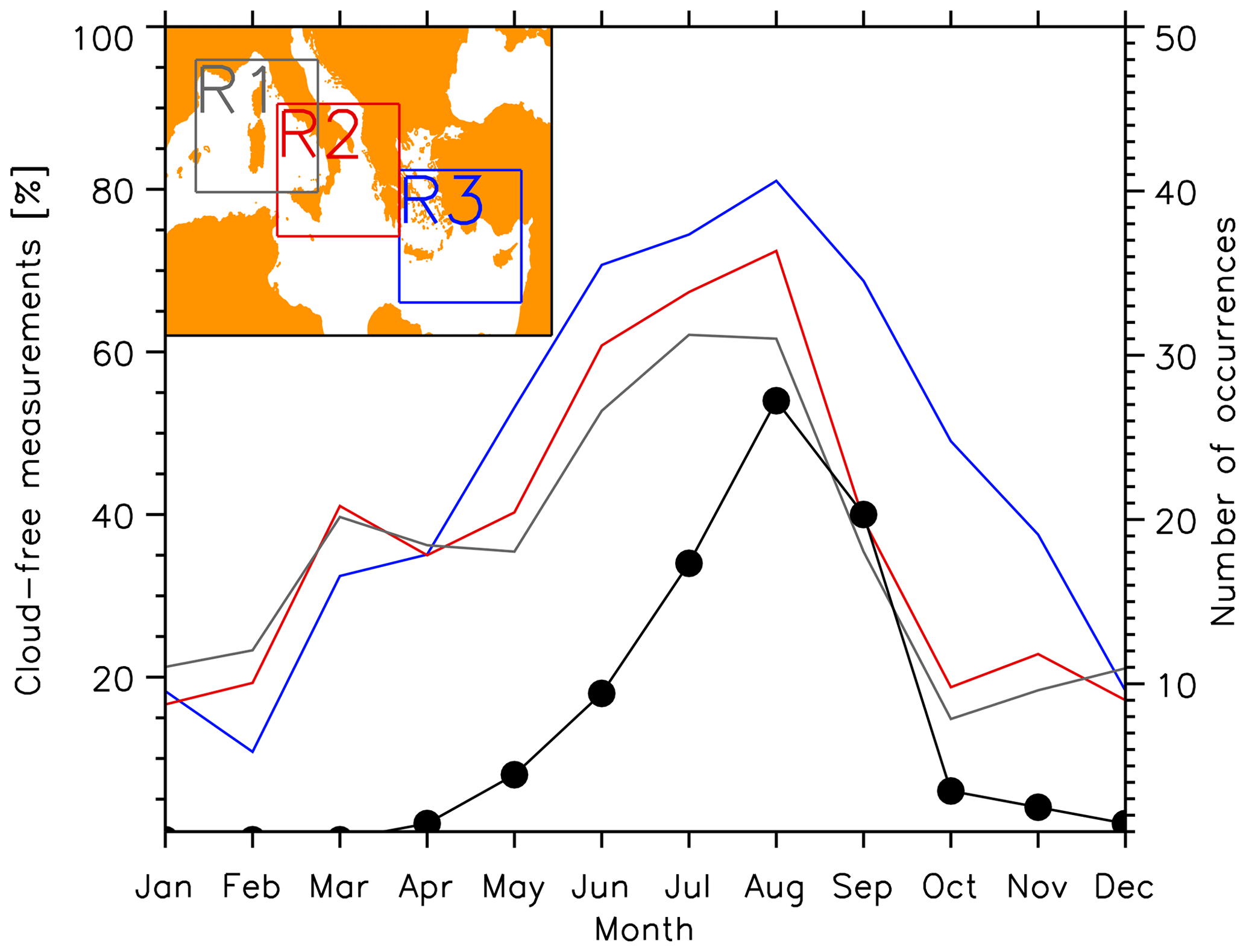
Figure 1Monthly means of the percentage of cloud-free measurements for the three corresponding areas (shown on the top-left map: R1 is grey, R2 is red and R3 is blue) for the year of 2003. The total number of lee wave occurrences (ATSR-2 + AATSR for the whole missions) is also reported as a function of the month (black curve, with the scale on the right-hand side).
Figure 1 shows the total number of monthly TCWV wave occurrences as a function of the month of the year (black curve). About 76 % of the selected cases are detected in JJA (June–July–August), 17 % are detected in MAM (March–April–May), and the remaining 7 % are detected in SON (September–October–November). Since we use only cloud-free measurements to detect the TCWV wave occurrences, the number of identified cases depends on the amount of available cloud-free data. In order to estimate the typical number of cloud-free pixels in each month, we performed an analysis using all the available AATSR measurements for the whole year of 2003. In Fig. 1 the monthly means of the percentage of cloud-free measurements are also plotted, using different colours according to the different geographical regions shown on the map. The highest number of available observations is found in August, in particular over the Eastern Mediterranean Sea (about 80 %), while the lowest observation amount is found in the winter (December–January–February – DJF; about 20 %), corresponding closely to the number of wave detections. One reason for the absence of TCWV wave occurrence in the winter months could be attributed to the frequent presence of lee waves accompanied by cloud.
The Aegean Sea is particularly suitable for the observation of these phenomena. From spring to fall, the northern Aegean is often crossed by the north-easterly Etesian winds (Kotroni et al., 2001; Miglietta et al., 2017), which change direction (becoming north-westerly or westerly) and intensify over the southern Aegean, approaching JJA monthly averages of about 8–10 m s−1 in parts of the Cyclades, parts of the Dodecanese Islands and to the east of Crete (e.g. Vagenas et al., 2017). Anticyclonic circulations, typical of summertime in the region, often yield clear-sky conditions. The complexity of the coastal orography and the presence of mountainous islands deeply influence the local-scale atmospheric circulation in the Ekman layer, producing effects at spatial scales down to a few kilometres (Vagenas et al., 2017).
As an example of TCWV wave detection, Fig. 2 shows the AATSR TCWV fields (Fig. 2a) and the corresponding NSD over the Aegean Sea (Fig. 2b) for 2 August 2002. In this figure, the wind speeds and directions, obtained from ERA-Interim products at a grid resolution of , are indicated with white arrows. The reported speeds have been derived using a linear interpolation over time of the 10 m (u and v) wind components, available every 6 h. Figure 2a clearly shows the lee wave structure of the AATSR TCWV, while Fig. 2b, showing the NSD, clearly demonstrated the correct geolocation of the lee wave area derived using our tool. In correspondence with the TCWV waves, the NSD value increases with respect to the background values, showing patterns clearly correlated with the wind direction. The used approach, which makes use, for simplicity, of a regular aggregation box size used to calculate the NSD, works almost uniformly for the majority of typical wavelengths. Nevertheless, small effects may arise both in case of wavelengths lower than half of the box size (wave effects are not completely resolved) or in case of wavelengths approaching the box size (only part of the wave is captured within the box), resulting in a decrease in the NSD value.
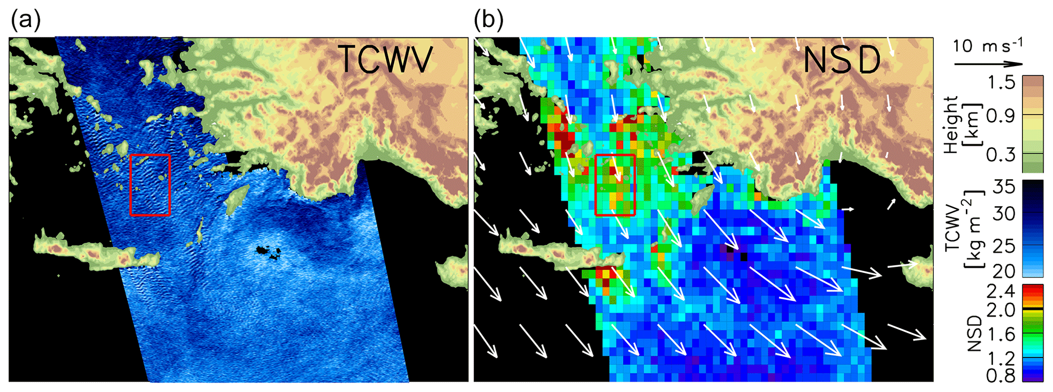
Figure 2(a) AIRWAVE TCWV for 2 August 2002 and AATSR orbit 2214 (ascending). (b) Corresponding normalised standard deviation. The arrows represent the wind speed (length) and direction, as derived from ERA-Interim products at resolution. The area delimited by the red box is studied more in detail in Fig. 4.
Several lee wave occurrences have been found close to the island of Crete, which has an elongated shape, spanning 260 km from east to west, while its north–south extension ranges from 12 to 60 km. The shape of the island and the presence of elevated mountain regions (up to 2450 m a.s.l.) generate wave-like patterns. Other occurrences have been found close to Sardinia and Corsica and near Cyprus.
Figure 3 shows the derived NSD for a set of selected lee wave events. Two cases are located between Sardinia, Corsica and the Italian Peninsula, over the Tyrrhenian Sea (Fig. 3g and h). One event is located in the Eastern Mediterranean across the island of Cyprus (Fig. 3f), and the remaining five are located over the Aegean Sea (Fig. 3a–e). In the figure, two cases are measured at two different times of the same day: Fig. 3a and b are obtained from, respectively, ERS-2 morning and evening satellite passes for the same day, with local crossing times at approximately 10:20 (descending) and 22:20 (ascending).
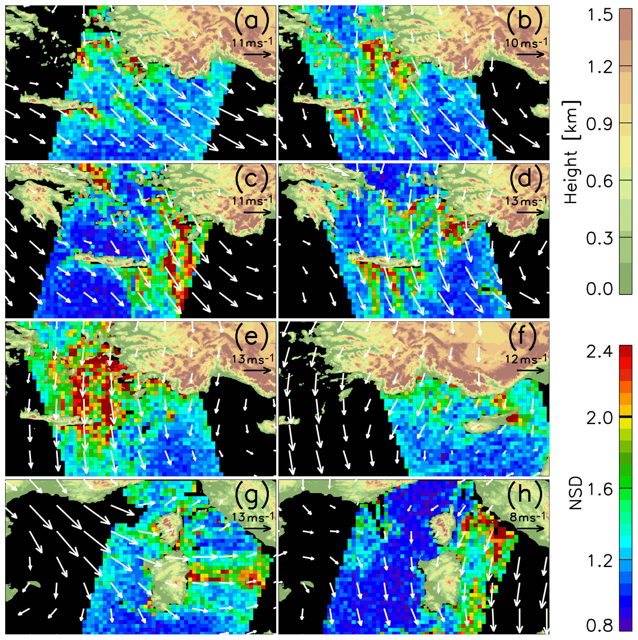
Figure 3Normalised standard deviation for (a) 23 July 1997, ATSR-2 orbit 11798 (descending); (b) 23 July 1997, ATSR-2 orbit 11805 (ascending); (c) 23 July 2002, ATSR-2 orbit 37936 (descending); (d) 26 April 2003, AATSR orbit 6036 (ascending); (e) 15 July 2009, AATSR orbit 38558 (ascending); (f) 19 June 2002, ATSR-2 orbit 37456 (ascending); (g) 2 August 2006, AATSR orbit 23121 (descending); and (h) 27 July 2002, ATSR-2 orbit 37994 (descending). The arrows represent the wind speed (length) and direction, as derived from ERA-Interim products at resolution.
The European Centre for Medium-Range Weather Forecasts (ECMWF) wind speeds for the selected events are shown with white arrows superimposed on the mapped NSD. The figure indicates that the patterns of the NSD are evidently correlated with the wind direction. The atmospheric conditions of the reported cases, all characterised by intense and constant wind direction, allowed the AGW propagation over long horizontal distances, trapping the wave vertically. Wind jets in the lee of mountain ranges may indeed generate horizontal waves which may propagate in a wave duct or wave guide horizontally over distances of even several hundreds of kilometres (Cheng and Alpers, 2010).
In order to find scientific evidence that the detected structures are indeed lee waves, we selected a subset of lee wave occurrences, and we compared them with both independent observations and model simulations. We found one particular case where the lee waves were measured almost simultaneously by two ATSR instruments. The comparison of the results of the detection algorithm applied to the two instruments enabled the assessment of its robustness, since each instrument has its own characteristics (e.g. noise and systematic errors) which may act in a different way in their measurements. This lee wave detection was then compared to the outputs of the WRF limited-area numerical model (see Sect. 3.1).
We also searched for SAR sea surface wind data co-located in time and space with AIRWAVE TCWV wave detections. We found one particular case suitable for our purposes from the ERS-2 SAR (see Sect. 3.2).
In all the aforementioned comparison exercises, we observed the presence of similar structures both in the AIRWAVE dataset and in the correlative data, thus enhancing the level of confidence of the detected AIRWAVE lee wave events (see Sect. 3.1).
The performed comparisons are illustrated in more detail in the following subsections.
3.1 ATSR-2 and AATSR near-simultaneous measurements and WRF model comparison
On 2 August 2002 the Aegean Sea area was observed by both ATSR-2 and AATSR with almost the same orbit track and a time separation of around 30 min. This “tandem” configuration offers an important opportunity to compare the TCWV products of the two sensors, which are similar in design but are characterised by different random and systematic measurement errors.
North-westerly winds were blowing with high intensity. Furthermore, the cloud masks of the two sensors indicate that the sky over the sea was almost entirely cloud-free. Our algorithm detected lee waves with similar spatial distributions from the TCWV fields derived from both sensors. In particular, the lee waves were located in the south-east of central Greece (Euboea Island) and of numerous Cyclades and Dodecanese islands (Andros; Tinos; Amorgos; Ikaria; Samos; Kos; and, to the south, up to Crete, Karpathos and Kassos), as can be seen in the TCWV fields and in the corresponding NSD map shown in Fig. 2.
We investigated, in more detail, the geographical area surrounded by the red box in Fig. 2. Figure 4a and b report the AIRWAVE TCWV values of this region for both ATSR-2 and AATSR, respectively. In this region, the island of Amorgos plays an important role in the development of the lee waves. Amorgos is a long and narrow island, with a length of 32 km and a width ranging between 1.9 and 5.5 km. It has relatively high, steep mountains (three of them over 500 m a.s.l.), located next to the sea. The wind direction on 2 August 2002 was almost perpendicular to the island main axis, as indicated by the ECMWF ERA-Interim wind speeds and directions, which are superimposed on the figure. These conditions led to the formation of observed trapped waves that extended several kilometres away from the source, clearly visible in the figure as alternate darker and lighter stripes. In Fig. 4, a very large correlation between the two AIRWAVE datasets can be noticed. This suggests that the observed pattern is real and not an artefact of a particular sensor.

Figure 4AIRWAVE TCWV (bluish colours) for 2 August 2002 over Aegean Sea, derived from ATSR-2, orbit 38086 (ascending), with measurements acquired from 20:11:41 to 20:12:00 (a), and AATSR, orbit 2214 (ascending), with measurements acquired from 19:43:11 to 19:43:30 (b). The black arrows represent wind speed (length) and direction, as derived from ERA-Interim fields interpolated at resolution. TCWV as computed from WRF model run (output at 20:00:00) is superimposed as white contour lines for two specific values of 29.2 and 30.5 kg m−2. The top-right box shows the satellite flight direction.
To strengthen the robustness of our analysis, we used the WRF model to simulate the atmospheric conditions of the sounded area. The Advanced Research WRF model (WRF-ARW version 3.5.1; Wang et al., 2010) was implemented with a grid spacing sufficient for the simulation of small-scale atmospheric waves. In this work, it was implemented in a one-way nested three-grid configuration, with 40 vertical levels and horizontal grid spacing, respectively, of 16, 4 and 1 km. 400×400 grid points are used in the inner domain, covering the area of 33.6–37.4∘ N, 24.7–29.2∘ E. ECMWF analysis and forecasts are used as initial and 3-hourly boundary conditions. The model simulation starts at 00:00 UTC, 2 August 2002, and lasts for 24 h so that the times of satellite observations are definitely after the model spin-up time. The following parameterisation schemes are employed: the Thompson et al. (2008) microphysics scheme, the rapid radiative transfer model (RRTM) for longwave radiation (Mlawer et al., 1997), the Dudhia (1989) scheme for shortwave radiation, the unified Noah land-surface model (Niu et al., 2011) and the Mellor–Yamada–Janjić scheme for the planetary boundary layer (Janjić, 2001). In the past, the model was successfully employed, with a similar configuration, to simulate wind speed in two case studies of orographic lee waves over the Eastern Mediterranean Sea in comparison with SAR retrieval (Miglietta et al., 2013).
In Fig. 4, the modelled vertically integrated water vapour values are superimposed on the ATSR TCWV fields (for the sake of image readability, only two contour levels are shown). The model foresees the presence of waves, with similar periodicity and direction to the ones detected by AIRWAVE, capturing very well the south-eastward lee waves extending from the Cyclades islands of Amorgos and Anafi. The presence of variability in a wave-like pattern in the lower troposphere was also confirmed from the WRF geopotential and temperature fields (not shown).
3.2 ATSR-2 and SAR comparison
An opportunity for comparison with independent correlative data was found for the event on 18 July 1997. On that day, the Tyrrhenian Sea region was observed by both the ATSR-2 instrument and the SAR instrument, both aboard ERS-2 satellite. Strong westerly winds blew across the island of Sardinia and over the Tyrrhenian Sea, with a direction and strength almost constant over the considered basin.
An enhancement of the NSD, derived from the ATSR-2 AIRWAVE TCWV fields of the ERS-2 orbit 11734, was detected in many grid cells of the considered region, as shown in Fig. 5a. The corresponding TCWV values, shown in Fig. 5b, show that the winds crossing Sardinia (from the ERA-Interim fields at ) clearly generate wave patterns over the sea, induced by the orography of the island. The formed lee waves propagate downstream for hundreds of kilometres in the Tyrrhenian Sea towards the Italian Peninsula. Once again, the NSD enhancements are largely correlated with the lee wave patterns in the TCWV fields. However some NSD values appear to be anomalously high, particularly in areas where there are missing data due to cloud. It may be that some thin cloud is missed in the ATSR mask, leading to error (increased variability) in the retrieved TCWV. A secondary cause may be the presence of clouds, reducing the number of elements that can be used within the grid cells. The observed TCWV fluctuations can be compared to the SAR wind fields, shown in the single-look complex images for the same day reported in Fig. 5c. The picture was obtained using the Earth Observation Link (EOLi; https://earth.esa.int/web/guest/eoli, last access: 20 November 2019), the European Space Agency's client for the Earth Observation Catalogue Service. The EOLi tool allowed the selection of Earth Observation products acquired by the ERS and ENVISAT satellites and the display of the related images on the top of an orthographic representation of the Earth. The service has been recently replaced by the ESA Simple Online Catalogue (https://esar-ds.eo.esa.int/oads/access/, last access: 20 November 2019).
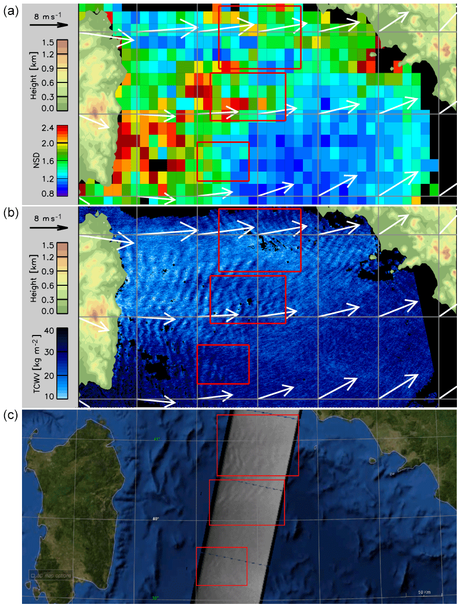
Figure 518 July 1997 over Tyrrhenian Sea. (a) NSD derived from the AIRWAVE TCWV fields (shown in b), ATSR-2, orbit 11734 (ascending), with measurements acquired at 21:14. The arrows represent the wind speed (length) and direction, as derived from ERA-Interim fields at resolution. (c) ERS-2 SAR single-look complex images; track 351; frames 2763, 2781, 2799 and 2817; and orbit 11728 (descending), with measurements acquired at 09:58.
The spatial resolution of the ERS-2 SAR images is very high: 26 m in range (across track) and between 6 and 30 m in azimuth (along track). The swath width of the sensor is about 100 km, thus covering only a portion of the AIRWAVE products in the longitude domain. The lee wave patterns shown in the SAR images downstream of the island of Sardinia reflect the sea surface impression of the perturbations in the lower troposphere. The patterns are in agreement with those derived from the AIRWAVE dataset. In particular, the geographical regions where the trapped lee waves are located are consistent between the two sensors (red boxes are shown in Fig. 5 as a guide).
As described in Sect. 2, the first step of our methodology consists of the detection of lee wave occurrence. Once the lee waves are found, it is useful to have a tool to provide quantitative information about the “local” wave characteristics, such as amplitude and wavelength estimated in different locations within the considered area. The fact that lee waves are stationary waves enables wave parameters to be recovered from the 2-D spatial patterns observed by satellites.
Small variations in the features induced by lee waves may occur, but their timescale is much longer than the duration of the satellite overpass so that they do not affect our results. We adopted the wavelet approach proposed by Torrence and Compo (1998), which was found to be suitable for characterising signals. The method used here is based on the Morlet CWT, a tool that can be used to analyse scale-dependent structures of a signal as it varies in time (or in space; Sadowsky, 1996). Several practical aspects of the analysis are reported in Torrence and Compo (1998), using time series of the El Niño–Southern Oscillation (ENSO) as a possible example of its application. The CWT approach has been successfully applied in several studies, e.g. for mesoscale gravity waves (Lu et al., 2005; Koch et al., 2005) and in the characterisation and removal of non-stationary and localised vertical structures in atmospheric temperature and density profiles retrieved from satellites (Iannone et al., 2014).
In this work, we used the wavelet software package, developed by Torrence and Compo (1998) in a series of different programming languages (available at http://paos.colorado.edu/research/wavelets/, last access: 20 November 2019). We applied the CWT method to the AIRWAVE TCWV fields shown in Fig. 4. The analysis was performed in the along-track direction (i.e. coincident with the satellite motion), which (in these cases) is nearly aligned with the wind direction and therefore with the wave pattern.
The method computes the energy of spectral components as a function of the along-track position (associated with a value of latitude, longitude and TCWV amount) and oscillation wavelength. For each along-track position, we then selected the wavelength corresponding to the most energetic wave. Repeating the analysis for each vector corresponding to a different across-track position, we obtained the results shown in Fig. 6. Figure 6a shows the analysis for the ATSR-2 orbit number 38086, while Fig. 6b shows that for the co-located AATSR orbit number 2214.
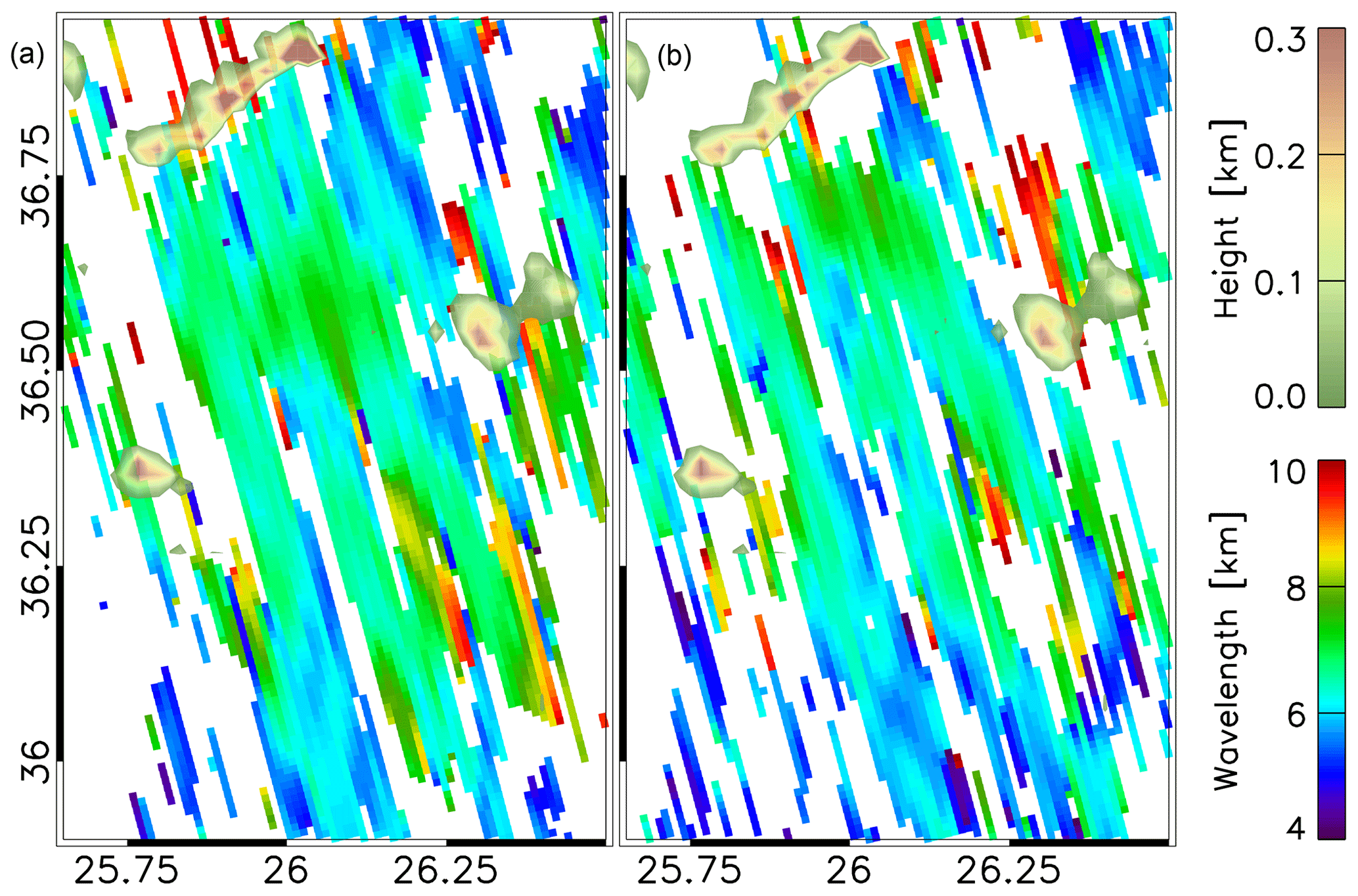
Figure 6Wavelength, indicated by the lower bar, with a colour scale ranging from 4 to 10 km, as derived by applying the CWT method to the AIRWAVE TCWV products shown in Fig. 4. (a) shows ATSR-2 orbit 38086 (ascending), and (b) shows AATSR orbit 2214 (ascending). The height of the ground is also shown (upper bar).
We considered only wave power values within the 95 % confidence interval, which is obtained by comparing the spectrum of individual wavelength series against a certain background level (the red noise; Torrence and Compo, 1998). Furthermore, we selected only wavelength values within the space–frequency region determined using the so-called cone of influence (COI), which is the region where the wavelet power spectra values can be considered unbiased by edge effects. The analysis shows that the majority of the TCWV fluctuations are statistically significant, both for AATSR and for ATSR-2. Wavelengths were detected mainly from 6 to 8 km (associated with azure–green colours in Fig. 6), with amplitudes of up to 75 % of the average TCWV amounts. Our findings are confirmed by the theoretical study performed by Nappo (2013). The paper states that the most energetic wavenumber kmax can be simply predicted using a mechanical approximation for lee wave development, assuming a spectrum of horizontal wavenumbers with kmax=4b, where b is the scale width of the mountain, computed as the distance between the maximum height and the point where the altitude reaches half of the maximum. Since the island of Amorgos is characterised by scale widths ranging from 1 to 2 km, this leads to a prediction of wavelengths ranging from 4 to 8 km, consistent with the wavelet analysis. Our method is analogous to the more rigorous Taylor–Goldstein approach described in Shutts (1997), whereby the wind and stability structure in the troposphere determines the resonant wavelength of the trapped wave.
We have identified lee wave occurrence over the Mediterranean Basin from the AIRWAVE total column water vapour dataset. The AIRWAVE data comprise about 20 years of daytime and nighttime products over water in clear-sky conditions, derived from the ATSR instrument series. The high (1 km×1 km) spatial resolution of the dataset is essential for the detection of these phenomena. We have investigated regions over the Tyrrhenian and Aegean seas, finding that the Greek basin is the place where lee waves are observed with the highest frequency due to its complex orography and coastlines and to the presence of intense winds and clear-sky conditions during most of the year. Lee waves have been found using an automatic tool that computes the TCWV standard deviation in spatial regions about 200–250 km2 wide and classifies the cases based on the number of clear-sky measurements and the derived normalised standard deviation.
We verified that the adopted method does not produce “false-positive” detections in regions where the presence of lee wave events is not expected (e.g. open ocean). The proposed approach has been intentionally kept simple; however some future improvements could be implemented, such as including in the detection algorithm the caveat of repetitive features in a short horizontal distance along the flow direction. We validated a subset of detected lee wave events, finding the presence of similar structures both in the AIRWAVE dataset and in the correlative data (independent observations or WRF model simulations).
Using the Morlet continuous wavelet transformation analysis, we were able to determine the characteristics of the observed lee waves in a region located south-west of the narrow island of Amorgos, finding wavelengths between 6 to 8 km, with amplitudes up to 75 % of the mean TCWV amount. The values are reasonable from a theoretical point of view and were confirmed by a WRF model run performed for the selected case. Therefore, the wavelength analysis approach adopted in this work has been found to be adequate. Nevertheless, we are investigating the possibility to develop a more sophisticated method for a statistical analysis of these events.
The proposed approach, which does not rely on external information, could in principle be applied to high-spatial-resolution TCWV products from other satellite instruments. The method is also very efficient from a computational point of view and is therefore suitable for near-real-time detection of lee waves from current flying sensors, e.g. the Sea and Land Surface Temperature Radiometer (SLSTR) and the Ocean and Land Color Instrument (OLCI), both aboard Copernicus Sentinel-3 (Donlon et al., 2012), and the two Moderate Resolution Imaging Spectroradiometer (MODIS) instruments aboard Terra and Aqua (Barnes and Salomonson, 1992). The tool could also be applied to other regions of the Earth. Future developments include a possible evaluation of radiative-forcing variations associated to wave events and a more accurate characterisation of the waves exploiting the tandem periods when measurements of two instruments almost overlap (e.g. Sentinel-3a SLSTR and Sentinel-3b SLSTR).
The AIRWAVE V2 data used in this work are available on request from the corresponding author.
EP, EC, SC and BMD conceived the method. MMM performed the WRF model simulations. EP performed the validation, performed the wavelet analysis and drafted the paper. All authors discussed the results and read and commented on the paper.
The authors declare that they have no conflict of interest.
We sincerely thank Richard Siddans for proofreading the article.
This paper was edited by Marcos Portabella and reviewed by two anonymous referees.
This research has been supported by ESA/ESRIN IDEAS+ (contract no. 4000108531/13/I-NB) and the funding from the European Commission (project “CEASELESS” (grant no. 730030)).
Barnes, W. L. and Salomonson, V. V.: MODIS: A global imaging spectroradiometer for the Earth Observing System, in: Optical Technologies for Aerospace Sensing: A Critical Review, International Society for Optics and Photonics, 10269, p. 102690G, https://doi.org/10.1117/12.161578, 1992. a
Casadio, S., Castelli, E., Papandrea, E., Dinelli, B. M., Pisacane, G., Burini, A., and Bojkov, B. R.: Total column water vapour from along track scanning radiometer series using thermal infrared dual view ocean cloud free measurements: The Advanced Infra-Red WAter Vapour Estimator (AIRWAVE) algorithm, Remote Sens. Environ., 172, 1–14, https://doi.org/10.1016/j.rse.2015.10.037, 2016. a, b
Castelli, E., Papandrea, E., Valeri, M., Greco, F. P., Ventrucci, M., Casadio, S., and Dinelli, B. M.: ITCZ trend analysis via Geodesic P-spline smoothing of the AIRWAVE TCWV and cloud frequency datasets, Atmos. Res., 214, 228–238, https://doi.org/10.1016/j.atmosres.2018.07.019, 2018a. a
Castelli, E., Miglietta, M. M., Dinelli, B. M., Stefano, C., Papandrea, E., and Bojkov, B.: Atmospheric Lee waves over the Eastern Mediterranean Basin as seen by the AIRWAVE Total Column Water Vapor and the WRF model, in: EUMETSAT Meteorological Satellite Conference 2018, Tallin, Estonia, 17–21 September 2018, 6.3_192, 2018b. a, b
Castelli, E., Papandrea, E., Di Roma, A., Dinelli, B. M., Casadio, S., and Bojkov, B.: The Advanced Infra-Red WAter Vapour Estimator (AIRWAVE) version 2: algorithm evolution, dataset description and performance improvements, Atmos. Meas. Tech., 12, 371–388, https://doi.org/10.5194/amt-12-371-2019, 2019. a, b, c
Cheng, C. M. and Alpers, W.: Investigation of trapped atmospheric gravity waves over the South China Sea using Envisat synthetic aperture radar images, Int. J. Remote Sens., 31, 4725–4742, https://doi.org/10.1080/01431161.2010.485145, 2010. a, b
Christie, D. R.: Solitary waves as aviation hazard, Eos T. Am. Geophys. Un., 64, 67–67, https://doi.org/10.1029/EO064i007p00067-01, 1983. a
Delderfield, J., Llewellyn-Jones, D. T., Bernard, R., De Javel, Y., Williamson, E. J., Mason, I., Pick, D. R., and Barton, I. J.: The along track scanning radiometer (ATSR) for ERS1, in: Instrumentation for optical remote sensing from space, International Society for Optics and Photonics, 589, 114–121, 1986. a
di Sarra, A., Fuà, D., and Meloni, D.: Estimate of surface direct radiative forcing of desert dust from atmospheric modulation of the aerosol optical depth, Atmos. Chem. Phys., 13, 5647–5654, https://doi.org/10.5194/acp-13-5647-2013, 2013. a
Donlon, C., Berruti, B., Buongiorno, A., Ferreira, M.-H., Féménias, P., Frerick, J., Goryl, P., Klein, U., Laur, H., Mavrocordatos, C., Nieke, J., Rebhan, H., Seitz, B., Stroede, J., and Sciarra, R.: The global monitoring for environment and security (GMES) sentinel-3 mission, Remote Sens. Environ., 120, 37–57, https://doi.org/10.1016/j.rse.2011.07.024, 2012. a
Dudhia, J.: Numerical study of convection observed during the winter monsoon experiment using a mesoscale two-dimensional model, J. Atmos. Sci., 46, 3077–3107, https://doi.org/10.1175/1520-0469(1989)046<3077:NSOCOD>2.0.CO;2, 1989. a
Gjevik, B. and Marthinsen, T.: Three-dimensional lee-wave pattern, Q. J. Roy. Meteor. Soc., 104, 947–957, https://doi.org/10.1002/qj.49710444207, 1978. a
Held, I. M. and Soden, B. J.: Water vapor feedback and global warming, Annu Rev. Energ. Env., 25, 441–475, https://doi.org/10.1146/annurev.energy.25.1.441, 2000. a
Iannone, R. Q., Casadio, S., and Bojkov, B.: A new method for the validation of the GOMOS high resolution temperature profiles products, Ann. Geophys.-Italy, 57, 0546, https://doi.org/10.4401/ag-6487, 2014. a
Jacob, D.: The role of water vapour in the atmosphere. A short overview from a climate modeller's point of view, Phys. Chem. Earth Pt. A 26, 523–527, https://doi.org/10.1016/S1464-1895(01)00094-1, 2001. a
Janjić, Z. I.: Nonsingular implementation of the Mellor-Yamada level 2.5 scheme in the NCEP Meso model, NCEP Tech. Rep., 437, 61 pp., available at: http://www2.mmm.ucar.edu/wrf/users/phys_refs/SURFACE_LAYER/eta_part4.pdf (last access: 20 November 2019), 2001. a
Koch, S. E., Jamison, B. D., Lu, C., Smith, T. L., Tollerud, E. I., Girz, C., Wang, N., Lane, T. P., Shapiro, M. A., Parrish, D. D., and Cooper, O. R.: Turbulence and gravity waves within an upper-level front, J. Atmos. Sci., 62, 3885–3908, https://doi.org/10.1175/JAS3574.1, 2005. a
Kotroni, V., Lagouvardos, K., and Lalas, D.: The effect of the island of Crete on the Etesian winds over the Aegean Sea, Q. J. Roy. Meteor. Soc., 127, 1917–1937, https://doi.org/10.1002/qj.49712757604, 2001. a
Li, X., Zheng, W., Yang, X., Li, Z., and Pichel, W. G.: Sea surface imprints of coastal mountain lee waves imaged by synthetic aperture radar, J. Geophys. Res., 116, C02014, https://doi.org/10.1029/2010JC006643, 2011. a
Lu, C., Koch, S. E., and Wang, N.: Stokes parameter analysis of a packet of turbulence-generating gravity waves, J. Geophys. Res., 110, D20105, https://doi.org/10.1029/2004JD005736, 2005. a
Lyapustin, A., Alexander, M. J., Ott, L., Molod, A., Holben, B., Susskind, J., and Wang, Y.: Observation of mountain lee waves with MODIS NIR column water vapor, Geophys. Res. Lett., 41, 710–716, https://doi.org/10.1002/2013GL058770, 2014. a, b
Miglietta, M. M., Zecchetto, S., and De Biasio, F.: WRF model and ASAR-retrieved 10 m wind field comparison in a case study over Eastern Mediterranean Sea, Adv. Sci. Res., 4, 83–88, https://doi.org/10.5194/asr-4-83-2010, 2010. a
Miglietta, M. M., Zecchetto, S., and De Biasio, F.: A comparison of WRF model simulations with SAR wind data in two case studies of orographic lee waves over the Eastern Mediterranean Sea, Atmos. Res., 120, 127–146, https://doi.org/10.1016/j.atmosres.2012.08.009, 2013. a
Miglietta, M. M., Huld, T., and Monforti-Ferrario, F.: Local complementarity of wind and solar energy resources over Europe: an assessment study from a meteorological perspective, J. Appl. Meteorol. Clim., 56, 217–234, https://doi.org/10.1175/JAMC-D-16-0031.1, 2017. a
Mlawer, E. J., Taubman, S. J., Brown, P. D., Iacono, M. J., and Clough, S. A.: Radiative transfer for inhomogeneous atmospheres: RRTM, a validated correlated-k model for the longwave, J. Geophys. Res., 102, 16663–16682, https://doi.org/10.1029/97JD00237, 1997. a
Nappo, C. J.: An introduction to atmospheric gravity waves, 2nd edn., Academic press, CJN Research Meteorology, Knoxville, Tennessee 37919, USA, 2013. a
Niu, G.-Y., Yang, Z.-L., Mitchell, K. E., Chen, F., Ek, M. B., Barlage, M., Kumar, A., Manning, K., Niyogi, D., Rosero, E., Tewari, M., and Xia, Y.: The community Noah land surface model with multiparameterization options (Noah-MP): 1. Model description and evaluation with local-scale measurements, J. Geophys. Res., 116, D12109, https://doi.org/10.1029/2010JD015139, 2011. a
Papandrea, E., Casadio, S., Castelli, E., Dinelli, B. M., De Grandis, E., and Bojkov, B.: Validation of the Advanced Infra-Red Water Vapour Estimator (AIRWAVE) Total Column Water Vapour using Satellite and Radiosonde products., Ann. Geophys.-Italy, 61, 1–8, https://doi.org/10.4401/ag-7524, 2018. a
Sadowsky, J.: Investigation of signal characteristics using the continuous wavelet transform, Johns Hopkins APL Technical Digest, 17, 258–269, 1996. a
Salomonson, V. V., Barnes, W., Xiong, J., Kempler, S., and Masuoka, E.: An overview of the Earth Observing System MODIS instrument and associated data systems performance, in: IEEE International Geoscience and Remote Sensing Symposium, IEEE, 2, 1174–1176, https://doi.org/10.1109/IGARSS.2002.1025812, 2002. a
Schröder, M., Lockhoff, M., Fell, F., Forsythe, J., Trent, T., Bennartz, R., Borbas, E., Bosilovich, M. G., Castelli, E., Hersbach, H., Kachi, M., Kobayashi, S., Kursinski, E. R., Loyola, D., Mears, C., Preusker, R., Rossow, W. B., and Saha, S.: The GEWEX Water Vapor Assessment archive of water vapour products from satellite observations and reanalyses, Earth Syst. Sci. Data, 10, 1093–1117, https://doi.org/10.5194/essd-10-1093-2018, 2018. a
Scorer, R. S.: Theory of waves in the lee of mountains, Q. J. Roy. Meteor. Soc., 75, 41–56, https://doi.org/10.1002/qj.49707532308, 1949. a
Shutts, G.: Operational lee wave forecasting, Meteorol. Appl., 4, 23–35, https://doi.org/10.1017/S1350482797000340, 1997. a
Teixeira, M. and Miranda, P.: Drag associated with 3D trapped lee waves over an axisymmetric obstacle in two-layer atmospheres, Q. J. Roy. Meteor. Soc., 143, 3244–3258, https://doi.org/10.1002/qj.3177, 2017. a
Teixeira, M. A., Argaín, J., and Miranda, P.: Drag produced by trapped lee waves and propagating mountain waves in a two-layer atmosphere, Q. J. Roy. Meteor. Soc., 139, 964–981, https://doi.org/10.1002/qj.2008, 2013. a
Teixeira, M. A., Paci, A., and Belleudy, A.: Drag produced by waves trapped at a density interface in nonhydrostatic flow over an axisymmetric hill, J. Atmos. Sci., 74, 1839–1857, https://doi.org/10.1175/JAS-D-16-0199.1, 2017. a
Thompson, G., Field, P. R., Rasmussen, R. M., and Hall, W. D.: Explicit forecasts of winter precipitation using an improved bulk microphysics scheme. Part II: Implementation of a new snow parameterization, Mon. Weather Rev., 136, 5095–5115, https://doi.org/10.1175/2008MWR2387.1, 2008. a
Torrence, C. and Compo, G. P.: A practical guide to wavelet analysis, B. Am. Meteorol. Soc., 79, 61–78, https://doi.org/10.1175/1520-0477(1998)079<0061:APGTWA>2.0.CO;2, 1998. a, b, c, d
Uhlenbrock, N. L., Bedka, K. M., Feltz, W. F., and Ackerman, S. A.: Mountain wave signatures in MODIS 6.7-μ m imagery and their relation to pilot reports of turbulence, Weather Forecast., 22, 662–670, https://doi.org/10.1175/WAF1007.1, 2007. a, b
Vagenas, C., Anagnostopoulou, C., and Tolika, K.: Climatic study of the marine surface wind field over the Greek seas with the use of a high resolution RCM focusing on extreme winds, Climate, 5, 29, https://doi.org/10.3390/cli5020029, 2017. a, b
Vosper, S. B., Sheridan, P. F., and Brown, A. R.: Flow separation and rotor formation beneath two-dimensional trapped lee waves, Q. J. Roy. Meteor. Soc., 132, 2415–2438, https://doi.org/10.1256/qj.05.174, 2006. a
Wang, W., Bruyère, C., Duda, M., Dudhia, J., Gill, D., Lin, H.-C., Michalakes, J., Rizvi, S., and Zhang, X.: ARW version 3 modelling system user's guide, NCAR, Boulder, Colorado, 312 pp., 2010. a
Wurtele, M. G., Datta, A., and Sharman, R. D.: Lee waves: Benign and malignant, NASA-CR-186024, Los Angeles, CA 90024-1565, 26 pp., available at: http://www.nasa.gov/centers/dryden/pdf/88288main_H-1890.pdf (last access: 20 November 2019), 1993. a
Wypych, A., Bochenek, B., and Różycki, M.: Atmospheric moisture content over Europe and the Northern Atlantic, Atmosphere, 9, 18, https://doi.org/10.3390/atmos9010018, 2018. a