the Creative Commons Attribution 4.0 License.
the Creative Commons Attribution 4.0 License.
 | 20 Dec 2019
High-precision atmospheric oxygen measurement comparisons between a newly built CRDS analyzer and existing measurement techniques
Tesfaye A. Berhanu
John Hoffnagle
Chris Rella
David Kimhak
Peter Nyfeler
Markus Leuenberger
Carbon dioxide and oxygen are tightly coupled in land biosphere CO2–O2 exchange processes, whereas they are not coupled in oceanic exchange. For this reason, atmospheric oxygen measurements can be used to constrain the global carbon cycle, especially oceanic uptake. However, accurately quantifying small (∼1–100 ppm) variations in O2 is analytically challenging due to the very large atmospheric background which constitutes about 20.9 % (∼209 500 ppm) of atmospheric air. Here we present a detailed description of a newly developed high-precision oxygen mixing ratio and isotopic composition analyzer (Picarro G2207) that is based on cavity ring-down spectroscopy (CRDS) as well as to its operating principles; we also demonstrate comprehensive laboratory and field studies using the abovementioned instrument. From the laboratory tests, we calculated a short-term precision (standard error of 1 min O2 mixing ratio measurements) of < 1 ppm for this analyzer based on measurements of eight standard gases analyzed for 2 h, respectively. In contrast to the currently existing techniques, the instrument has an excellent long-term stability; therefore, calibration every 12 h is sufficient to get an overall uncertainty of < 5 ppm. Measurements of ambient air were also conducted at the Jungfraujoch high-altitude research station and the Beromünster tall tower in Switzerland. At both sites, we observed opposing and diurnally varying CO2 and O2 profiles due to different processes such as combustion, photosynthesis, and respiration. Based on the combined measurements at Beromünster tower, we determined height-dependent O2:CO2 oxidation ratios varying between −0.98 and −1.60; these ratios increased with the height of the tower inlet, possibly due to different source contributions such as natural gas combustion, which has a high oxidation ratio, and biological processes, which have oxidation ratios that are relatively lower.
- Article
(3945 KB) - Full-text XML
- BibTeX
- EndNote


Atmospheric oxygen comprises about 20.9 % of the global atmosphere, and over the past decade its concentration has decreased at a rate of ∼20 per meg yr−1 (Keeling and Manning, 2014) which has mainly been associated with the increase in fossil fuel combustion. Measurements of atmospheric O2 are reported as the ratio of the O2 concentration to the N2 concentration: expressed as δ(O2∕N2). This is due to the fact that variations in the concentrations of other atmospheric gases, such as CO2, can influence the O2 partial pressure, whereas the abovementioned ratio is insensitive to changes in other gases. Atmospheric O2 is commonly expressed in units of per meg due to its small variability with respect to a large background, where
Equation (1) is used to convert oxygen mole fraction changes expressed in parts per million (as measured by several techniques such as paramagnetic cell, UV cell, and the CRDS analyzer presented here) into changes in δO2∕N2. This is associated with the influence of dilution effects on the mole fractions but not necessarily on the ratios. These conversion difficulties and their expressions in uncertainties are discussed in the Appendix. In contrast to O2, the global average atmospheric CO2 mixing ratio has increased to 405.0 ppm averaged over 2017 from its preindustrial value of 280 ppm (Le Quéré et al., 2018). As the variability of atmospheric oxygen is directly linked to the carbon cycle, both its short- and long-term observations can be used to better constrain the carbon cycle. For example, since it was first suggested by Keeling and Shertz (1992), the long-term trends derived from concurrent measurements of atmospheric CO2 and O2 have been widely used to quantify the partitioning of atmospheric CO2 between the land biosphere and oceanic sinks (Battle et al., 2000; Goto et al., 2017; Manning and Keeling, 2006; Valentino et al., 2008). This method hinges on the linear coupling between CO2 and O2 with an oxidation ratio (OR; defined as the stoichiometric ratio of exchange during various process such as photosynthesis and respiration and expressed using α) of 1.1 for the terrestrial biosphere photosynthesis–respiration processes (αb) and 1.4 for fossil fuel combustion (αf), whereas they are decoupled for oceanic processes. Meanwhile, the short-term variability in atmospheric oxygen can be used to estimate marine biological productivity and air–sea gas exchange (Keeling et al., 1998; Nevison et al., 2012). However, the accuracy of these estimates is primarily linked to the accuracy and precision of atmospheric O2 measurements and the assumed ORs for the different processes that are highly variable in contrast to atmospheric CO2, which can be well measured within the precision guidelines set by the Global Atmospheric Watch (GAW; ±0.1 ppm for the Northern Hemisphere).
Currently there are several, mostly custom-built, techniques that can measure atmospheric O2 variations as the oxygen concentration, based on interferometric, paramagnetic, UV absorption, and fuel cell technology (Keeling, 1988a; Manning et al., 1999; Stephens et al., 2007), or as O2∕N2 ratios to account for the large background effect, using gas chromatography with thermal conductivity detector (GC-TCD) or gas chromatography coupled to mass spectrometry (GC-MS) (Bender et al., 1994; Tohjima, 2000). Despite the fact that these techniques have been used for more than 2 decades, accurate quantification of atmospheric oxygen variability remains challenging; this is primarily because the small atmospheric oxygen signal (in parts per million) rides on a ∼210 000 ppm background, which places stringent requirements on the precision and drift of the analysis methods – especially for continuous monitoring (note that the GAW recommendation for the measurement precision of O2∕N2 is 2 per meg). The techniques listed above struggle to routinely achieve the necessary performance for various reasons, including (i) instability over time that requires frequent measurement interruption for calibration, (ii) measurement bias with respect to ambient and sample temperature and/or pressure, and/or (iii) systematic errors in the measurement due to other atmospheric species. Furthermore, some techniques require the use of consumables and rely on high vacuum, which complicates field deployment.
In this paper we describe a new high-precision oxygen concentration and isotopic composition analyzer by Picarro Inc., Santa Clara, USA (G2207) based on CRDS technology. Here, we will introduce the analyzer design principles in detail, describe the unique features of the analyzer, and evaluate its performance based on various independent laboratory and field tests by comparing it with currently existing techniques. We will then present and interpret our observations based on field measurements. Finally, we will present conclusions on its overall performance and provide recommendations and possible improvements.
The analyzer described here is derived from the Picarro G2000 series of CRDS analyzers. The basic elements have been described elsewhere (Crosson, 2008; Martin et al., 2016; Steig et al., 2014); briefly, the instrument is built around a high-finesse, traveling-wave optical cavity, which is coupled to one of two single-frequency distributed feedback-stabilized semiconductor lasers. One cavity mirror is mounted on a piezoelectric translator (PZT) to allow fine tuning of the cavity resonance frequencies. A semiconductor optical amplifier between the laser sources and the cavity boosts the laser power and serves as a fast optical switch. The cavity body is constructed of invar and enclosed in a temperature-stabilized box (T=45 ∘C, stabilized to approximately 0.01 ∘C) for dimensional and spectroscopic stability. A vacuum pump pulls the gas to be sampled through the cavity, and a proportional valve between the cavity and the pump maintains the sample pressure in the cavity at a value of 340 hPa, with variations of the order of 1 Pa. The instrument has a wavelength monitor, based upon measurements of interference fringes from a solid etalon, which is used to control the laser wavelength by adjusting the laser temperature and current. The wavelength monitor is a fiber-coupled device located between the laser and the cavity. A fraction of the beam from the input fiber is collected using a beam splitter for the wavelength measurement and the remaining power is collected in the output fiber. A high-speed photodiode monitors the optical power emerging from the cavity. The instrument's data acquisition system sweeps the laser frequency over the spectral feature to be measured, modulates the laser output to initiate ring-downs, and fits the ring-down signal to an exponential function to generate a spectrogram of optical loss versus laser frequency. For this instrument the empty cavity ring-down time constant is about 39 µs. Subsequent program modules compare the measured loss spectrum to a spectral model, using nonlinear least-squares fitting (Press et al., 1986) to find the best-fit model parameters; thus, they obtain a quantitative measure of the absorption due to the target molecule, and finally apply a calibration factor to the optical absorption to deduce the molecular concentration. When operating in its normal gas analysis mode, the instrument acquires about 200–300 ring-downs per second and typically achieves a noise equivalent absorption of about 10−11 cm−1 Hz, with some variation between instruments.
The primary goal when designing this analyzer was to measure the molecular oxygen concentration with a few-per-meg level of precision and stability. In this context operational stability is as important as the signal-to-noise ratio. Our experience has been that the most stable operation of the analyzer is achieved when the optical phase length of the cavity is held as constant as possible. In this case the free spectral range (FSR; 0.0206 cm−1) of the temperature-stabilized, invar ring-down cavity provides a better optical frequency standard than the etalon-based wavelength monitor, which in turn allows for more consistent measurements of the absorption line width and integrated absorption line intensity (Steig et al., 2014). For a small, field-deployable instrument, it is not practical to stabilize the absolute frequencies of the cavity modes to an optical frequency standard (Hodges et al., 2004); however, the oxygen lines themselves, under conditions of constant temperature and pressure, provide an adequate frequency reference. The oxygen spectrum was also used to calibrate the FSR by comparing a wide (approximately 10 cm−1) FSR-spaced spectrum with the HITRAN database (Gordon et al., 2016).
To determine the molecular oxygen concentration, the analyzer measures absorption of the Q13Q13 component of the band, at 7878.805547 cm−1, according to the latest edition of HITRAN (Gordon et al., 2017). This is one of the strongest near-infrared lines of oxygen, well separated from other oxygen lines, and is reasonably free of spectral interference from water, carbon dioxide, methane, and other constituents of clean air. The spectral model for this line was developed using reference spectra of clean, dry, synthetic air that were acquired with the same hardware as in the field-deployable analyzer, but with specialized software that allows it to operate as a more general spectrometer.
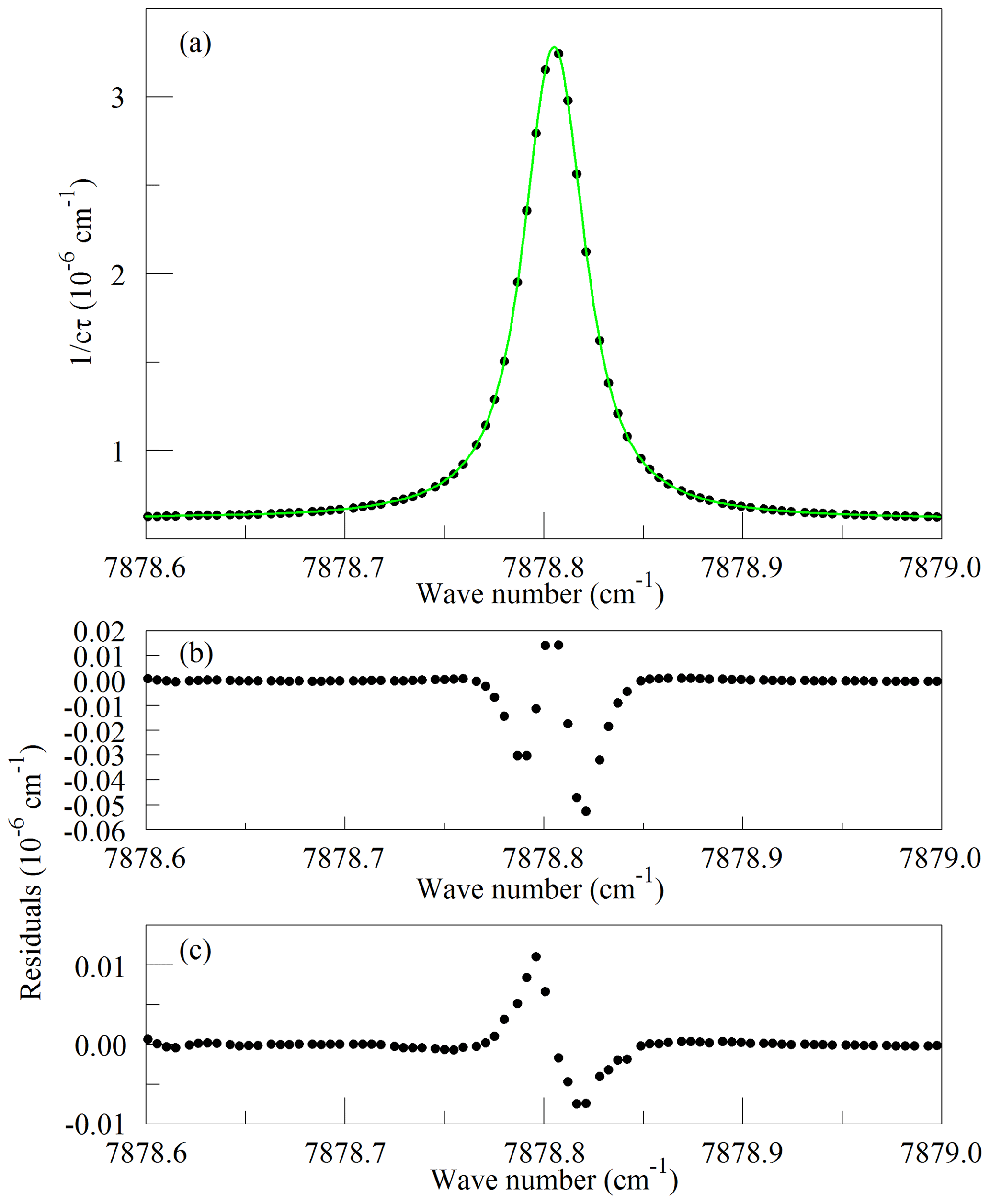
Figure 1Panel (a) shows the raw data (points) and the best-fit Galatry function (solid line); residuals of the Voigt fit are shown in panel (b); and residuals of the Galatry fit are shown in panel (c).
Recently, considerable work has been carried out to advance the understanding of spectral line shapes and to define functional representations that better describe the processes that determine spectral line shapes than the Voigt model does (Hartmann et al., 2008; Tennyson et al., 2014; Tran et al., 2019). Line shape studies have been published for the 1.27 µm band of O2 (Lamouroux et al., 2014), although not to our knowledge for the Q branch. The apparatus used here is not capable of spectroscopic studies of comparable precision; the absolute temperature and pressure monitoring and especially the frequency metrology are far too crude for that purpose. Our goal is merely to define a simple model of the Q13Q13 line that is adequate for least-squares retrievals of the O2 absorption under the limited range of conditions (stabilized temperature and pressure) that the operational analyzer experiences in the field. The CRDS analyzers use the Galatry function (Varghese and Hanson, 1984), which is distinctly better than the Voigt and is still easily and quickly evaluated for line shape modeling. Ultimately, the usefulness of the spectral model is to be evaluated by the precision and stability of the O2 measurements when compared with established techniques. For spectral model development, this spectrometer has the drawback that the cavity FSR is too large to reveal much detail of the absorption line shape, even with the simplifying assumption of a Galatry line shape. Therefore, we acquired a set of four interleaved spectra, with the PZT-actuated mirror moved to offset the cavity modes of the individual FSR-spaced spectra by one-fourth of an FSR. The precise offsets were determined from fits to the strong and well-isolated O2 lines in the spectra. From the consistency of the fitted line centers, we estimate that the positioning of the interleaved spectra was accurate to approximately 10 MHz. The spectrum of the Q13Q13 line acquired in this manner is shown in Fig. 1, along with the best-fit Galatry function. It stands out that the residuals are largely odd in detuning from the line center: this shows the limitations of the Galatry model in this case, as the Galatry function is purely even about the line center. The shape of the absorption line in this model is specified by two dimensionless parameters: the collisional broadening parameter
and the collisional narrowing parameter
where γ is the frequency of broadening transitions, β is the velocity change collision rate, and σD is the 1∕e Doppler half-width of the transition; the latter is given by
where ν0 is the transition frequency, kB is the Boltzmann constant (J K−1), T is the sample temperature (K), M is the molecular mass (amu), and c is the speed of light (m s−1). Figure 2 shows the values of y and z obtained from spectra acquired in the same way as in Fig. 1, as a function of cavity pressure. The values depend linearly on pressure, as expected from the Galatry model, but the unconstrained linear fits do not pass precisely through the origin. It is not clear whether this represents a breakdown of the Galatry model or simply reflects the limited quality of the data set. The slope of y can be converted to an air-broadened collisional width γair=0.0442 cm−1 atm−1, which agrees with the HITRAN value of 0.0460 cm−1 atm−1 (Gordon et al., 2016) to within the uncertainty estimate stated by HITRAN (uncertainty code 4 for γair corresponding to 10 %–20 % relative uncertainty). The slope of z can be interpreted in terms of the optical diffusion coefficient (Fleisher et al., 2015), yielding D=0.285 cm2 s−1, compared with the literature value of 0.233 cm2 s−1 for O2 in air at 45 ∘C (Marrero and Mason, 1972). Although the anticipated use of the analyzer is for ambient air samples with a very small range of O2 concentrations, we did investigate the variation of the line shape in binary mixtures of O2 and N2 (shown in Fig. 3). The error bars are taken from the output of the Levenberg–Marquardt fitting routine (Press et al., 1992). The dependence of the collisional broadening parameter z on O2 mole fraction was considered to be too small to be significant, but the variation in y was used in the subsequent analysis of the air samples. Note that Wójtewicz et al. (2014) also found collisional broadening coefficients for nitrogen to be slightly larger than for oxygen in measurements of one O2 line in the B-band.
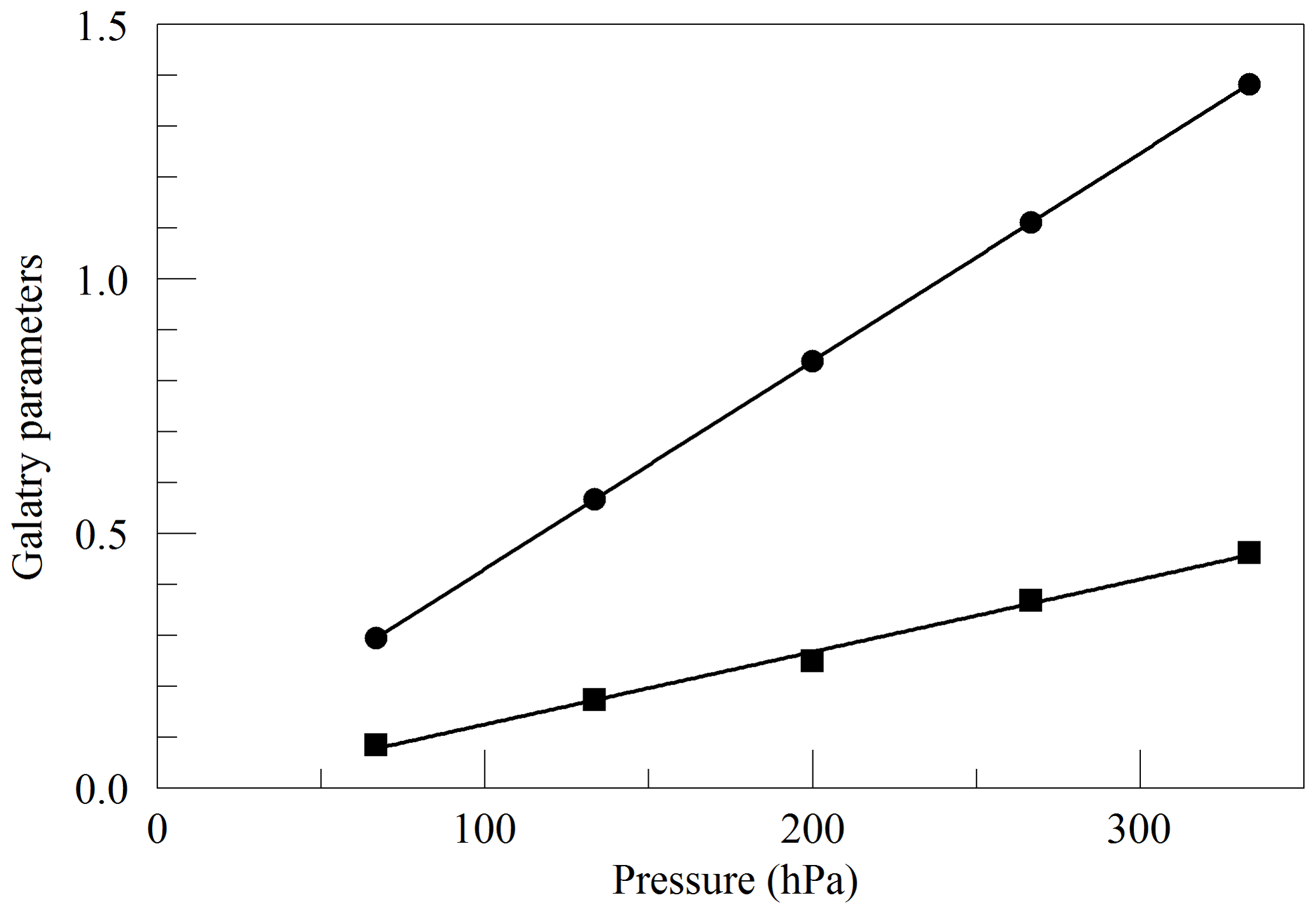
Figure 2Best-fit values for the Galatry parameters of the Q13Q13 line of O2, as a function of pressure. The line broadening parameter y is represented by circles, and the line narrowing parameter z is represented by squares. The solid lines are linear fits to the measurements. The respective best-fit offset and slope are 0.0227 and 0.004082 hPa−1 for y, and −0.0169 and 0.001424 hPa−1 for z.
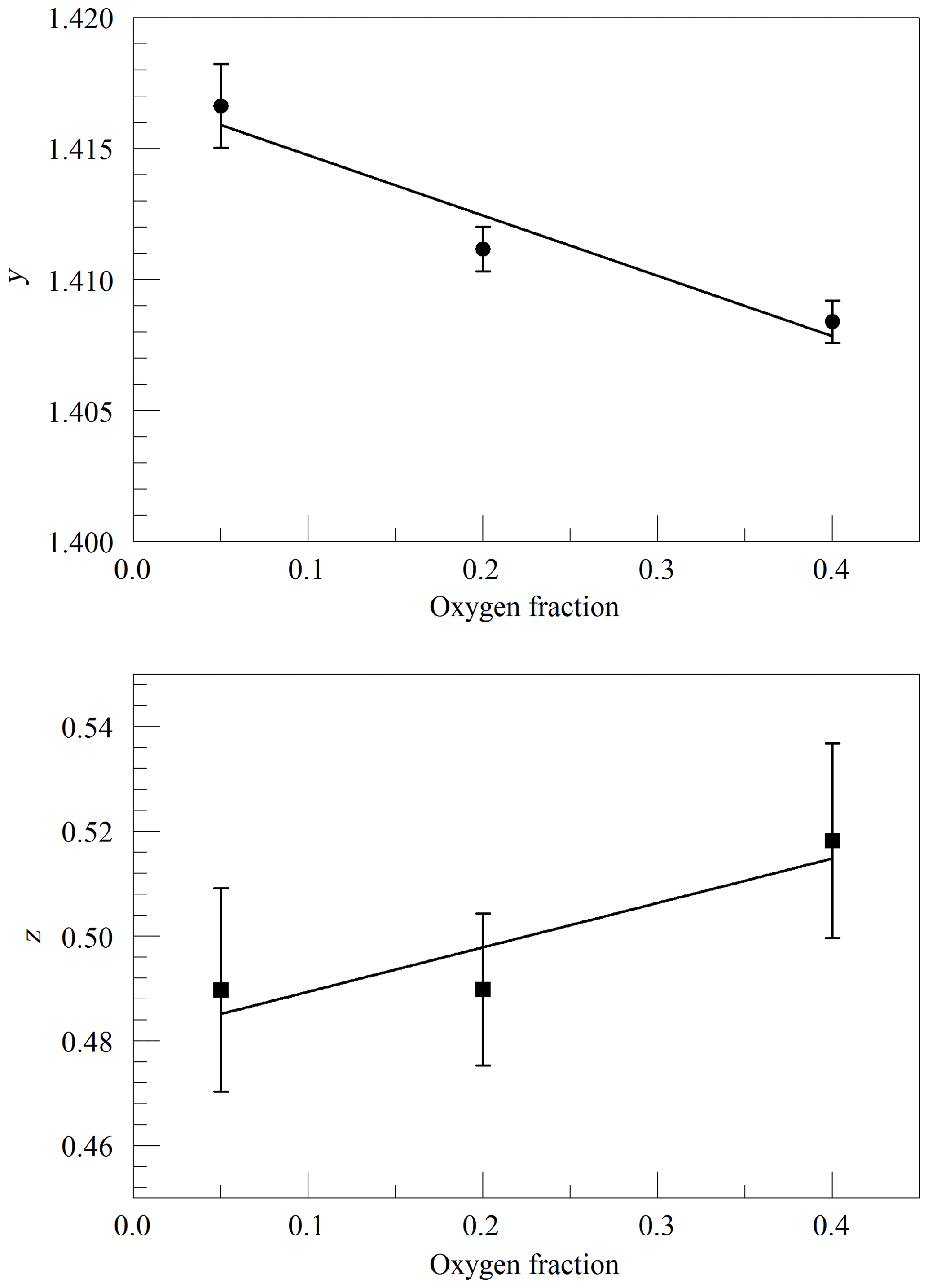
Figure 3Galatry parameters of the Q13Q13 line of O2 at 340 hPa and 45 ∘C as a function of the O2 mole fraction in binary O2–N2 mixtures. The linear fits to the data are and .
The primary goal in designing the analyzer was to achieve high enough precision to make meaningful measurements of O2 in clean atmospheric samples. Although the current best practice for such high-precision measurements is to work with dried samples, we decided to include high-precision measurements of water vapor. There were two reasons for this decision: one was to serve as a monitor for residual water vapor, which is difficult to remove completely from the ring-down cavity and associated sample handling hardware, and the second and more ambitious reason was to see how well the effect of water vapor could be corrected for measurements of undried ambient air. While it was considered unlikely that measurements of undried air could compete with those of dried air with respect to accuracy, it might be possible to correct for water vapor well enough to enable useful measurements in some circumstances without the expense and inconvenience of drying the sample. For this purpose, a second laser was added, which probed the component of the 2v3 band of water vapor, at of 7816.75210 cm−1 (Gordon et al., 2017). The Galatry model was used to fit spectra of synthetic air humidified to various levels of water vapor concentration. These fits also included two other nearby, very weak water lines, with intensities of less than 1 % of the strong transition, so that their absorption would not perturb the line shape of the main transition. Results for the shape of the 7816.75210 cm−1 line are shown in Fig. 4. At the level that we can measure, only the y parameter has a meaningful variation with water concentration. From the linear fit, one obtains a pressure broadening coefficient for air, γair=0.0752 cm−1 atm−1, which is in reasonable agreement with the HITRAN value γair=0.0787 cm−1 atm−1 (Gordon et al., 2017), and a self-broadening coefficient, γself=0.413 cm−1 atm−1, to be compared with the HITRAN value of γself=0.366 cm−1 atm−1. As the uncertainty estimate for the HITRAN values is 10 %–20 %, this level of agreement seems reasonable.
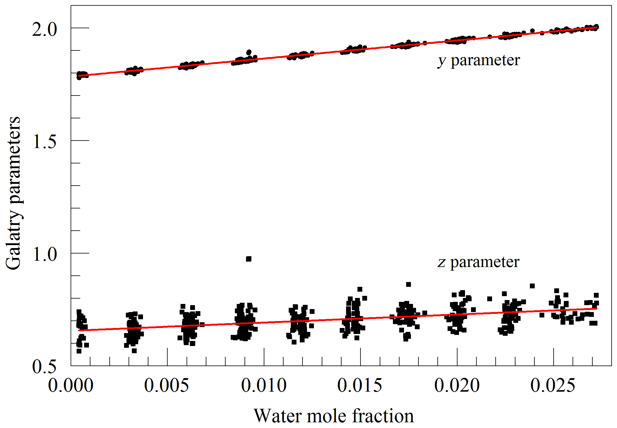
Figure 4Galatry parameters of the 7816.75210 cm−1 water line in air at 340 hPa and 45 ∘C as a function of water mole fraction. Black points are from measurements and red lines are linear fits of and .
We also looked at absorption from water near the Q13Q13 absorption line of O2. These spectra were measured on a background of pure nitrogen to reveal the very weak lines interfering with the O2 measurement. Without the strong O2 lines, it was impossible to interleave FSR-spaced spectra; therefore, in this case, the frequency axis comes from the analyzer's wavelength monitor. Figure 5a shows the spectrum of saturated water vapor in nitrogen and a fit to a Voigt model of the molecular lines. The measurement was made at a pressure of 340 hPa and a temperature of 45 ∘C. The main features are the Q13Q13 line from the trace contamination of oxygen in the sample and several lines that arise from normal water () and deuterated water (1H2H16O also abbreviated HDO). Figure 5b shows the lines tabulated in HITRAN. Immediately after the data in Fig. 5 were acquired, measurements were also made at 7816.85210 cm−1 to establish the relationship between the absorption strengths in the two spectral regions. The relative intensities of the H2O and HDO lines change with variations in the isotopic composition of the water, but fortunately the direct interference with the oxygen Q13Q13 lines stems entirely from the H2O isotopologue, with the strongest HDO line being separated by approximately 8 line widths (full width at half maximum) from the Q13Q13 line. HITRAN simulations for molecules other than water that are expected to be present in clean, ambient air indicate that direct interference with the Q13Q13 line should be negligible at the level of precision considered here. In the case of CO2, the dilution of oxygen due to 400 ppm of CO2 is significant, and larger than any direct spectral interference.
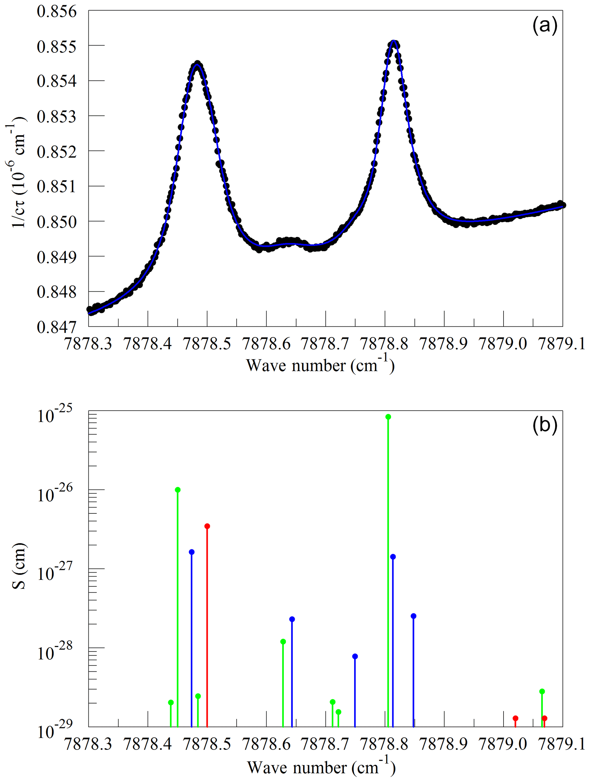
Figure 5(a) Spectrum of water in nitrogen (points) and fit to the Voigt model (blue curve). (b) Oxygen (green), normal water (blue), and deuterated water (red) lines in the 2016 HITRAN database.
Finally, we investigated the influence of water vapor on the shape of the O2 Q13Q13 line. Switching between the two lasers sources, we acquired FSR-spaced spectra of humidified synthetic air, alternately covering the 7817 and 7878 cm−1 regions. Individual spectra were acquired in less than 2 s, so changes in water vapor concentration between spectra were small. These spectra, with a frequency resolution of 0.0206 cm−1, were analyzed by nonlinear least-squares fitting with the following spectral models: the 7817 cm−1 spectra were modeled as the sum of an empty-cavity baseline with an adjustable offset level and slope, and the water spectrum was modeled with three peaks – one strong line and two weak perturbers. The molecular absorption of the main peak was expressed as an adjustable amplitude, Aw, multiplying a dimensionless, area-normalized Galatry function (Varghese and Hanson, 1984). The weak perturbers were modeled by Voigt profiles with amplitudes and line widths that were constrained to be in fixed proportions with the strong line, and therefore added no new degrees of freedom to the fitting procedure. As the amplitude Aw multiplies an area-normalized shape function, it is essentially equivalent to the area of the absorption line, to the extent that the Galatry model provides a valid description of the line shape. The Doppler width of the Galatry function was fixed based on the measured cell temperature, the y parameter was allowed to vary, and the z parameter was constrained to be proportional to y, based on measurements summarized in Fig. 2. In addition, the center frequency of the Galatry function was adjusted to match the data set, giving a total of five free parameters for this fit. The 7878 cm−1 spectra were modeled with an adjustable baseline offset and slope and a molecular absorption amplitude, , describing the Q13Q13 O2 line. Here, the y parameter and line center position of the O2 lines were also allowed to adjust, and the z parameter was constrained to be proportional to y. The weak water lines interfering with oxygen absorption were included in the model, but with no additional free parameters; rather the amplitudes were preset based on the measured water absorption at 7817 cm−1 and the previously determined amplitude relationships between the water lines. This procedure does not account for variations in HDO abundance, which may introduce some systematic error into the water vapor correction for samples of unusual isotopic composition, but it should accurately model the most important lines that interfere with the oxygen measurement. Collisional broadening of the Q13Q13 O2 line by water vapor is shown in Fig. 6. From the linear fit, one obtains a coefficient for collisional broadening of the Q13Q13 line by water vapor of γwater=0.0442 cm−1 atm−1 at 45 ∘C. Recently, parameters describing the broadening of oxygen lines by water vapor, obtained by empirical modeling of selected experimental data, were added to the HITRAN database (Tan et al., 2019). The new HITRAN entries predict a value of 0.0486 cm−1 atm−1 at 45 ∘C, which is in agreement with our measurement within the 5 %–10 % uncertainty attributed by HITRAN to the broadening parameter. The alternating measurements at 7817 and 7878 cm−1 also calibrated the relationship between the water mole fraction and the absorption at 7817 cm−1, using a dilution analysis described by Filges et al. (2018), who showed that the results obtained this way agree well with water vapor fractions measured with a conventional hygrometer. Figure 7 shows the measured amplitudes of the water and oxygen lines for samples of variable humidity. As the air came from a tank of constant composition, the oxygen concentration changes due to dilution of oxygen when water is added. Assuming that this is the sole cause of the change in measured absorption, as the line shapes were being constantly adjusted to account for changes in collisional broadening, it is straightforward to deduce the relation between the water fraction and the absorption amplitude. This calibration was used to generate the water fraction axes in Figs. 4 and 6. We note that we did not take particular care to control or measure the quantity of dissolved gases, especially oxygen and carbon dioxide, in the water used for this experiment. While these gases would not significantly affect the water calibration, they may affect the water vapor correction of the oxygen measurement at the part per million level. More work needs to be carried out to investigate the water vapor correction of the oxygen measurement.
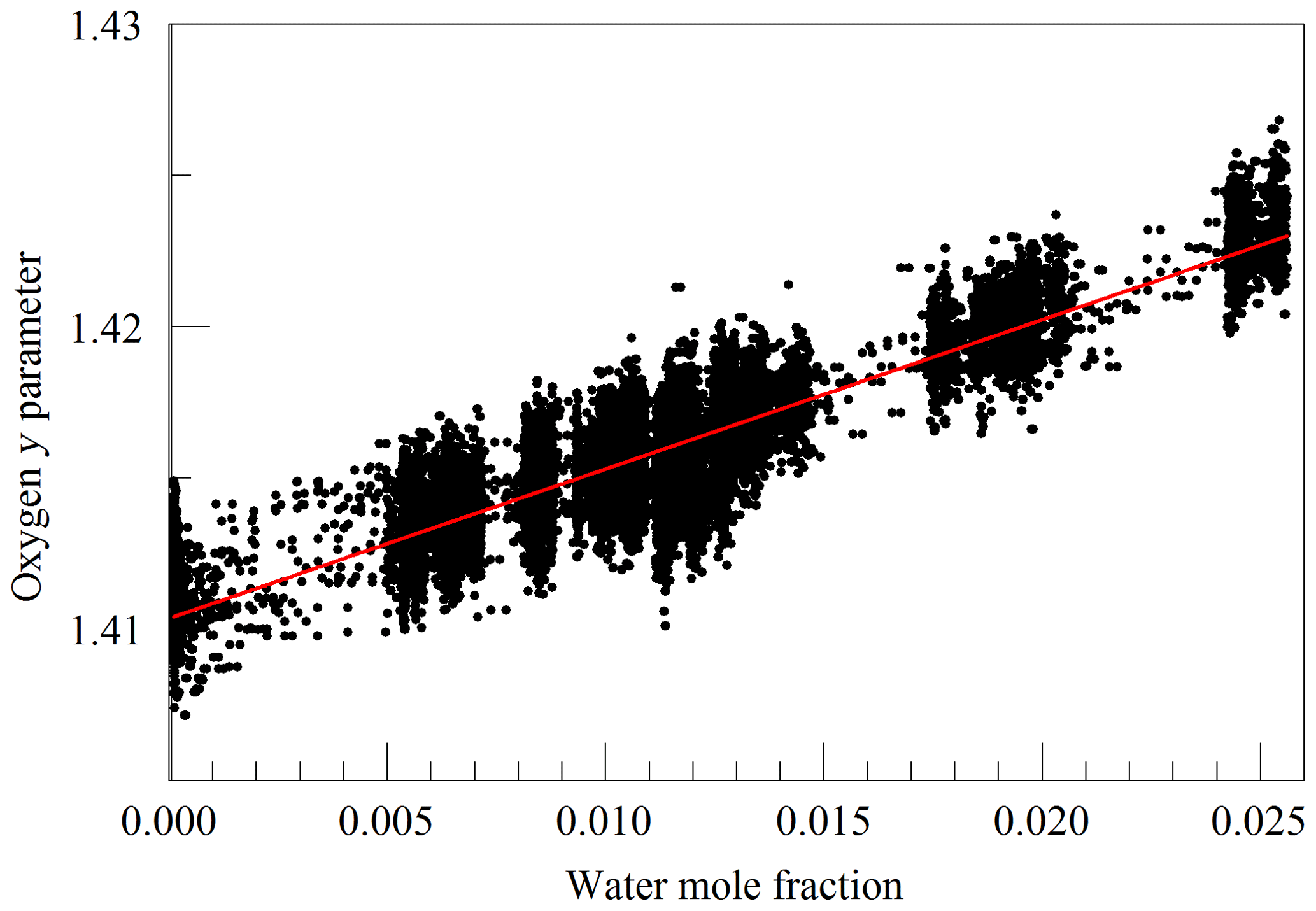
Figure 6Galatry collisional broadening parameter of the oxygen Q13Q13 line at 340 hPa and 45 ∘C versus the water mole fraction. Black points are from measurements and the red line is a linear fit of .

Figure 7Measured absorption line amplitudes for oxygen and water vapor for water vapor mixing ratios ranging from nearly 0 to 0.025. Black points are from measurements and the red line is a linear fit with an intercept of cm−1 and a slope of −0.014807.
The observations described above were used to design a method to measure oxygen concentration in ambient air. Gas from the inlet to the analyzer is drawn through the cavity at a rate of about 100 sccm (standard cubic centimeters per minute) and the conditions in the cavity are held stable at 340 hPa and 45 ∘C. In its analysis mode the analyzer alternately measures ring-downs in the respective 7817 and 7878 cm−1 regions. At 7878 cm−1 measurements are made at 11 different frequencies, spaced by one FSR of the cavity and centered at the peak of the Q13Q13 line. Multiple ring-down measurements are made to improve the precision of the loss determination, with a total of 305 ring-downs allocated to one spectrum. In the 7817 cm−1 region measurements are also made at 11 distinct frequencies at FSR spacings. Only 35 ring-downs are allocated to this spectral region, as the measurement of O2 is much more important than water vapor. The data sets are analyzed using a Levenberg–Marquardt fitting routine, which adjusts five free parameters in each region to find the best agreement to a spectral model based on Galatry line shapes, as described above. One of the outputs of the 7878 cm−1 fit is the frequency offset of the FSR grid from the center of the Q13Q13 line. This information is used to adjust the position of the PZT-actuated mirror to keep the measurements centered on the line, effectively stabilizing the optical path length of the cavity to the frequency of the O2 line. The reported water fraction is obtained by multiplying the fitted amplitude of the water line by a calibration constant derived from the dilution experiment, as explained above. For the O2 fraction a slightly more complicated procedure is followed. It was observed that the least-squares fitting of the data gives highly correlated results for the amplitude of the absorption line and the line width parameter y. The correlation may be due in part to covariance of the fitted amplitude (proportional to line area) and line width (Press et al., 1992) and it may also have a contribution from pressure variations that the pressure sensor is unable to detect. The ratio can be determined from the fit much more precisely than alone and therefore gives a more sensitive measurement of molecular absorption. It also has the advantage of being independent of sample pressure, to the extent that the Galatry model applies (Fig. 2). However, using the ratio as a metric for absorption adds more complications if measurements are to be made over a range of O2 and water concentrations, because the O2∕N2 ratio and the water concentration affect the line width independently of pressure and O2 concentration alone. To minimize systematic errors due to these broadening effects, we define a nominal y parameter based on the measured amplitudes of the O2 and water lines and the line broadening dependences shown in Figs. 3 and 4. The measured ratio is multiplied by the nominal y to obtain a quantity that is ideally independent of pressure and water concentration, and this is the quantity that is multiplied by a calibration constant to give the reported O2 fraction. In addition, a dry mole fraction is reported for O2, which is defined as the directly measured mole fraction corrected for water dilution.
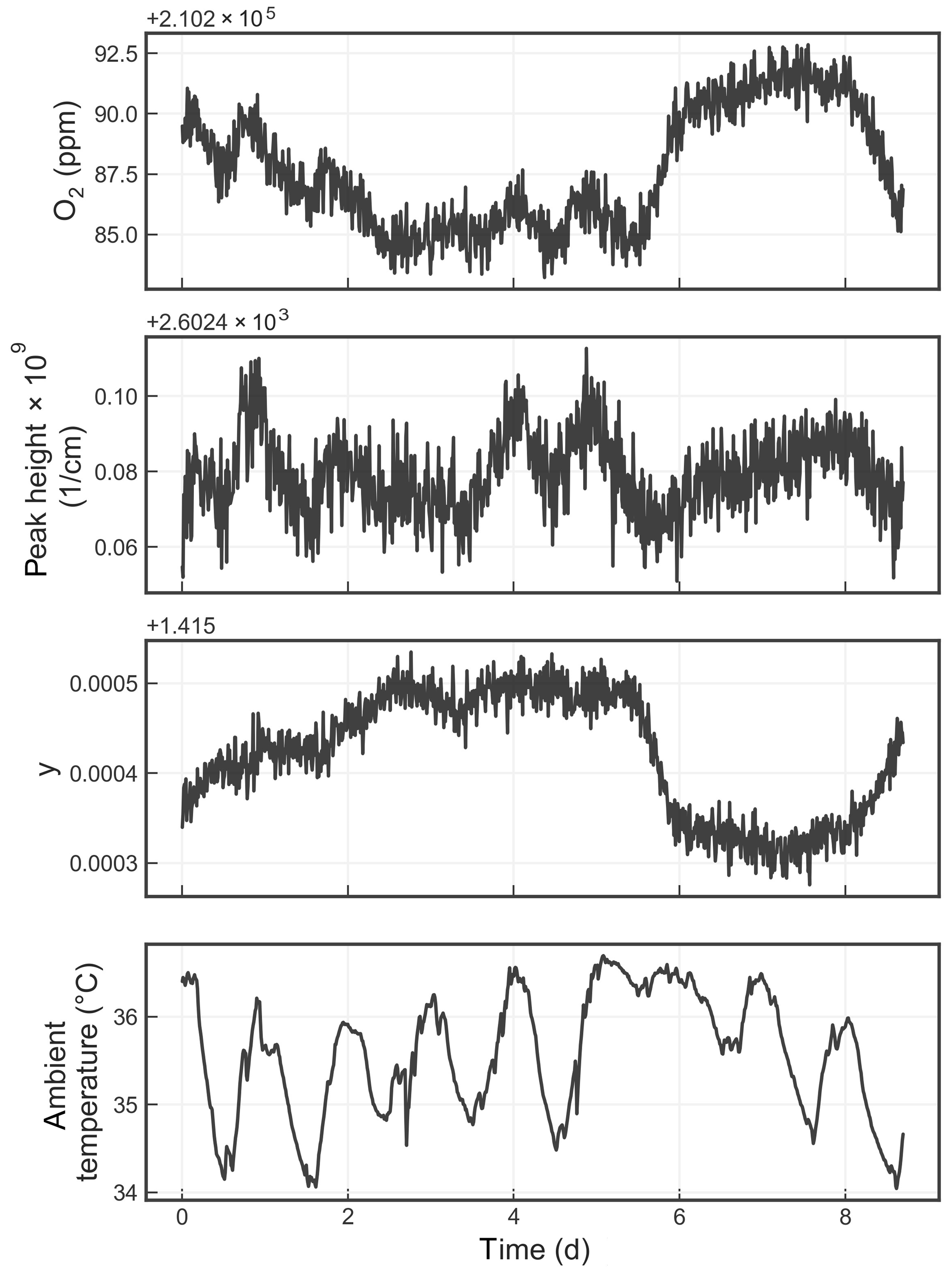
Figure 8Time series from a measurement of a single tank over about a week. The four panels show the water-corrected oxygen concentration, the absorption peak loss minus the baseline loss, the measured Lorentzian broadening factor, and the ambient temperature (measured in the instrument housing), respectively. A windowed average of 300 s was applied to all four data sets.
The main goal in developing this instrument was to make high-precision measurements of the O2 mole fraction, based on absorption by the dominant 16O2 isotopologue. The absorption lines of the rarer isotopologues are also present nearby; therefore, a mode of operation was included in which one laser is scanned over neighboring lines of 16O2 and 16O18O and the ratio of amplitudes is used to derive an isotopic ratio, reported in the usual delta notation. In this case the operating pressure was reduced to 160 hPa to improve the resolution of the nearby lines. The lines measured were the Q3Q3 line of 16O2, at 7882.18670 cm−1, and the Q9Q9 line of 16O18O, at 7882.050155 cm−1. The measurement procedure is very similar that of the O2 fraction measurement, so it will not be described in detail and only the main differences will be noted. One is that in determining an isotopic ratio, normalizing absorption amplitudes by line widths does not provide any advantage, instead we simply take the ratio of amplitudes to compute delta. Although the Q9Q9 line and its neighbor Q8Q8 are the strongest ones in this band, absorption by 16O18O is still very weak – only about cm−1 at the line center under the conditions we used. The signal-to-noise ratio that can be achieved with this analyzer is not adequate to determine both the amplitude and the width of the 16O18O line with useful precision; thus, in the fitting step, the y parameter of the 16O18O line is constrained to be a constant factor times the fitted y parameter for the 16O2 line. Additionally, because of the weakness of the rare isotopologue absorption, the majority of ring-downs in each spectrum is devoted to measuring 16O18O, i.e., 232 ring-downs in each spectrum versus only 40 for 16O2. This implies that the mole fraction measurement in the isotopic mode is much less precise than when the analyzer measures the Q13Q13 line alone.
3.1 Laboratory tests at Picarro, Santa Clara
3.1.1 Temperature and pressure sensitivity
One set of tests was carried out to determine how well the goal of minimizing the susceptibility of the concentration measurements to noise or drift of the sample temperature and pressure was met. For these tests the analyzer sampled dry synthetic air from a tank, and the temperature and pressure set points of the cavity were adjusted upward and downward from the nominal values in order to obtain an estimate of the differential response. We express the sensitivity to experimental conditions in relative form: the derivative with respect to temperature or pressure divided by the signal under nominal conditions.
From these experiments, we determined a temperature sensitivity of K−1 and a pressure sensitivity of hPa−1. The temperature sensitivity is somewhat larger than expected based on a calculation using HITRAN data to estimate the temperature dependences of all the quantities that go into the measured absorption of the Q13Q13 line. The pressure sensitivity is strikingly small, indicating a good cancelation of the pressure dependence of the absorption amplitude and line width. Both temperature and pressure sensitivities are small enough to have a negligible effect on the short-term precision of measurements made with the stabilized ring-down cavity, although long-term drifts in the sensors are always a matter of concern.
3.1.2 Measurement precision and drift
Measurement precision was evaluated by analyzing synthetic air containing nominal atmospheric concentrations of CO2 and CH4 from an aluminum Luxfer cylinder over a period of several days. The tank, oriented horizontally and thermally insulated (although not controlled), was connected directly to the instrument (S/N TADS2001) with a two-stage pressure regulator and stainless-steel tubing with an additional orifice of about 55 sccm. For the isotopic mode of operation, the precision of the measurement was also tested by making repeated measurements from a tank of clean, dry synthetic air.
Figure 8 shows the time series of the precision test data, displaying the reported oxygen concentration, the height of the oxygen absorption peak, the width of the oxygen absorption peak, and the ambient temperature. The residual error of the analyzer, although small, is still significant given the stringent targets set forth by the WMO-GAW program. Possible sources of error include temperature drifts due to sensor drift or gradients; pressure errors due to sensor drift; and optical artifacts such as parasitic reflections, higher-order cavity mode excitation, and/or a loss of nonlinearity that can distort the reported oxygen spectrum. More work is required to identify and eliminate these small drifts.
The Allan standard deviation of the reported O2 fraction is shown in the Allan–Werle plot in Fig. 9. The ordinate on this plot is the square root of the Allan variance of the reported mole fraction, so 1 ppm in these units corresponds to about 5 per meg in the O2∕N2 ratio. The precision of averaged measurements improves as for approximately 5000 s, reaches 1 ppm in less than 10 min, and remains below 1 ppm for timescales of the order of about 1 h (τ is the averaging time, which is the abscissa of the Allan–Werle plot).
Figure 10 shows the precision of δ(18O) (uncalibrated) derived from the ratio of lines measured at 7882 cm−1. Because of the weak signal from the 16O18O line, it is necessary to average for 20 s or more to achieve 1 ‰ precision for the isotopic ratio. As for the concentration measurement, averaging improves the measurement precision for timescales up to about 1 h.
Table 1Assigned mixing ratios of standard gases used in this study and their corresponding values measured by the NDIR, CRDS, and IRMS at the University of Bern.
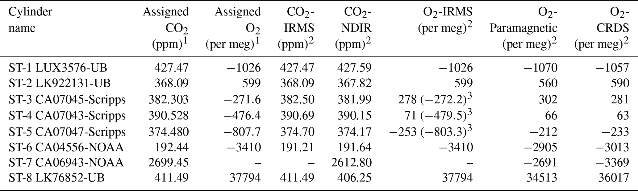
1 The assigned values are based on measurements from different institutions (University of Bern (UB), Scripps, or NOAA; see column cylinder name). 2 Measurements are on the Bern scale for CO2 and O2. The Bern scale is shifted by +550 per meg. 3 Values on the Scripps scale.
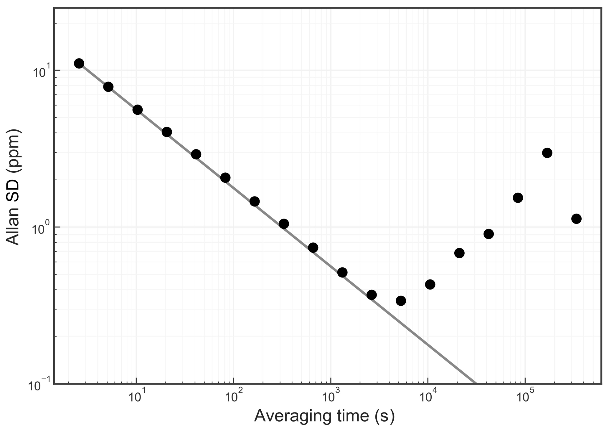
Figure 9Precision of the O2 mole fraction measured from a tank of synthetic air. Filled circles are measurements and the line shows the ideal dependence.
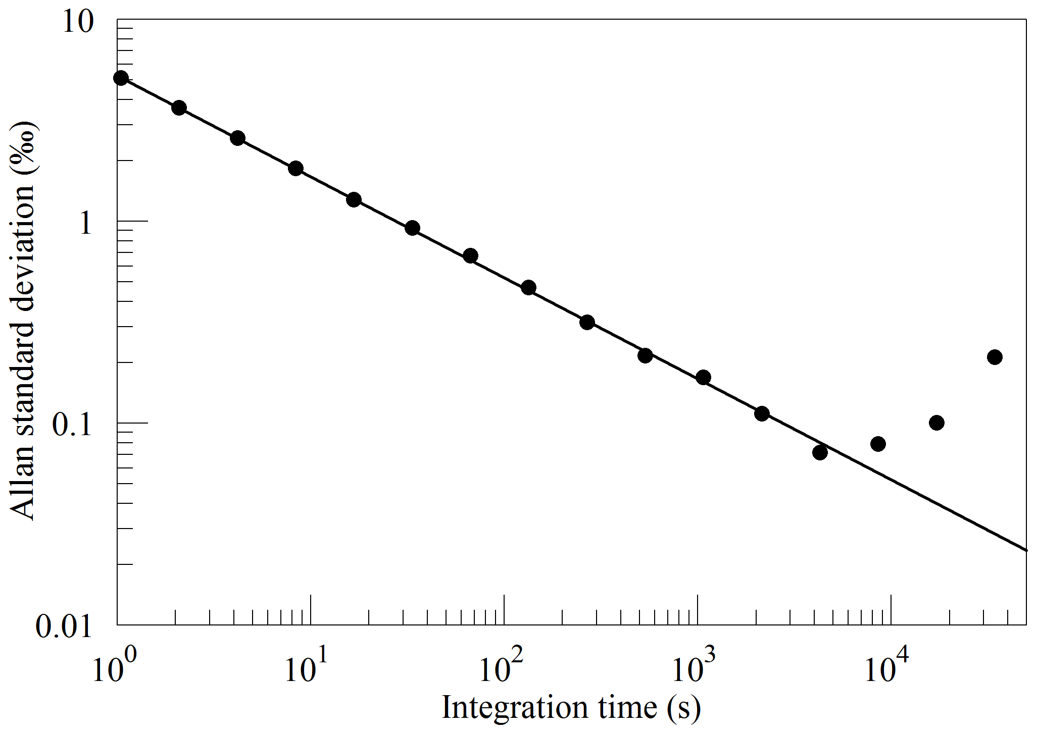
Figure 10Precision of δ(18O) measured from a tank of synthetic air. Filled circles are measurements and the line shows the ideal dependence.
3.2 Laboratory measurements at the University of Bern
3.2.1 Measurements of standard gases
The performance of the instrument was tested by analyzing eight standard gases with precisely known CO2 and O2 compositions (Table 1) using the CRDS analyzer. These values were then compared to parallel measurements with a paramagnetic oxygen sensor (PM1155 oxygen transducer, Servomex Ltd, UK) embedded to a commercially available fuel cell oxygen analyzer (OXZILLA II, Sable Systems International, USA) (Sturm et al., 2006) as well as with an isotope ratio mass spectrometer (IRMS, Finnigan DeltaPlusXP). The design of the measurement setup is shown in Fig. 11. Standard gases were directly connected to the pressure controlling unit, and a multi-port valve (V2) was used to select among the standard gases. Flow from each cylinder was adjusted to about 120 sccm and was eventually directed to a selection valve (V1), allowing for switching between ambient air and standard gases. Flow towards and out of the fuel cell analyzer was controlled by the pressure controlling unit. The O2 mixing ratio of this incoming gas was first measured on the paramagnetic oxygen sensor and then directed towards a nondispersive infrared analyzer (NDIR; Li-7000, LICOR, USA) to measure CO2 and H2O. The outflow from this analyzer (100 sccm) returns to the pressure controlling unit and was eventually divided between the CRDS analyzer (which uses about 75–80 sccm) and the IRMS (∼20 sccm) via a tee junction. Each cylinder was measured for 2 h in each system and controlled by a LabVIEW program.
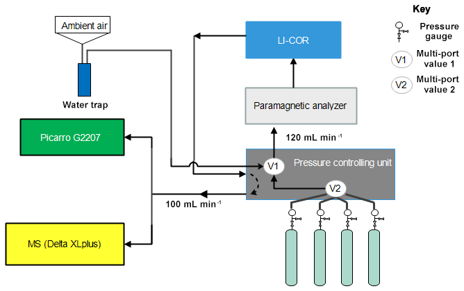
Figure 11Schematics of the measurement system used to compare the Picarro analyzer with the mass spectrometer at Bern.
First, we investigated the influence of this tee junction, which splits the gas flow between the CRDS and the IRMS, on the measured O2 values. Manning (2001) showed that the fractionation of O2 in the presence of a tee junction is strongly dependent on the splitting ratios as well as temperature and pressure gradients. Hence, we measured and compared the O2 mixing ratios of two standard gases (CA07045 and CA060943) in two cases: (i) in the presence of a tee junction with different CRDS to IRMS splitting ratios and (ii) without a tee junction so that all gas flow is directed towards the CRDS analyzer. The splitting ratios in these test experiments varied from 1:1 to 1:100, and reversed to change the major flow direction either to the CRDS or the IRMS. Note that the experimental condition in this paper is a 4:1 splitting ratio (i.e., approximately 80 sccm towards the CRDS analyzer and approximately 20 sccm towards the IRMS).
In the cases of smaller splitting ratios (1:1, 1:4, and 4:1), which are relevant for the results presented in this study, only minor differences in the measured O2 mixing ratios were observed when compared to case (ii) (i.e., without a tee junction). For the two cylinders measured, the average differences in these cases were about 0.5 ppm, calculated as the mean of the differences in the raw O2 measurements of the last 60 s. The negligible fractionation can indeed be the result of smaller splitting ratios, whereas strong influence is usually expected for larger splitting ratios (Stephens et al., 2007). For higher splitting ratios, the result seems inconclusive without any dependence on the ratios due to the strong decline in the cylinder temperature (specifically at the pressure gauge) caused by higher flow to achieve the higher splitting ratios (as high as 1:100). Hence, these tests need to be conducted under temperature-controlled conditions, and the results could not be discussed in this paper.

Figure 12Comparison of oxygen mixing ratios for the seven standard gases measured using the CRDS analyzer (black) and the paramagnetic sensors (red).
Figure 12 shows the standard gas measurements for the seven cylinders with known CO2 and O2 mixing ratios (Table 1) using both the CRDS and the paramagnetic analyzers. Standard 8, which has an overly high O2 content, is not shown in the figure as the figure is zoomed-in to better illustrate the change in O2 for the remaining cylinders. While the first five cylinders contain O2 and CO2 mole fractions comparable to ambient air values, standards 6 and 8 either had very low or very high O2, respectively. In addition, standards 6 and 7 had very low and very high CO2 mixing ratios, respectively. Note that due to its very high CO2 content (approximately 2700 ppm), standard 7 was not measured on the IRMS; hence, its O2 mixing ratio is unknown. The measured mixing ratios for the six standard gases measured with the two systems are in very good agreement, whereas cylinder 7 showed an inverse signal for the two analyzers compared with standard 6 (Fig. 12). While the paramagnetic analyzer showed a higher O2 mixing ratio, the values from the CRDS analyzer are lower in O2. This could be associated with the very high CO2 mixing ratio in standard 7, which leads to a strong dilution effect in the CRDS analyzer as it does not include any correction function for the dilution effect from CO2. However, such high CO2 mixing ratios may not be that important in most atmospheric research. Yet, including an additional laser to this analyzer in order measure the CO2 mixing ratio in parallel should be considered important, as it will further improve the accuracy of the oxygen measurements. This would be especially important for biological or physiological studies where a wide range of CO2 and O2 concentrations must be expected.
The measurement precision of the CRDS analyzer was calculated as the standard error of the mean, i.e., the standard deviation (1σ) of the last 1 min raw measurements divided by the square root of the number of measurements (n=60); for all of these cylinders the values were usually between 0.5 and 0.7 ppm. For parallel measurements of these cylinders using a paramagnetic analyzer, we obtained a precision of about 1 ppm, calculated in exactly the same way.
We also made a correlation plot to see which of the two instruments was in better agreement with the assigned values based on IRMS measurements for the individual cylinders. While similar correlation coefficients were observed for both analyzers, different slopes were calculated (Fig. A1). This is due to the fact that the IRMS measures the O2 to N2 ratio (δ(O2∕N2)) in per meg, whereas the CRDS and the paramagnetic analyzers provide non-calibrated O2 mixing ratios in parts per million and per meg, respectively. If we exclude the two standard gases with the highest and lowest O2 mixing ratios (standards 7 and 8) that are subjected to strong dilution effects, both the slope and the r2 values decrease from those shown in Fig. A1. However, this decrease is larger in the case of the paramagnetic measurements, implying a slightly better linearity of the CRDS analyzer.
Furthermore, the slope between the IRMS and CRDS O2 values in Fig. A1 corresponds to 5.78 per meg ppm−1, which is significantly larger than the conversion factor of 4.78 per meg ppm−1 as derived from Eq. (1) assuming a constant N2 content. This higher slope is due to the dilution effect originating from any gas component change (Δ, given in parts per million) on all air components of air samples, which has not been corrected for in the CRDS values. When accounting for this dilution effect – that scales with – the factor approaches 4.78 per meg ppm−1. The scaling of the dilution effects is independent of which air component is changing and it affects all air components in a similar fashion relative to their molecular fractions. Oxygen values measured using a CRDS or paramagnetic cell instrument are affected even if there is no change in O2 or N2 but there is a change in CO2, water vapor, or any other component that is present. This is in contrast to measurements of O2∕N2 ratios for the same case where an equal ratio would be measured. Major dilution influences are expected from O2, CO2, and H2O changes due to natural exchange processes on air samples or when using artificial air-like compositions.
3.2.2 Measurements of ambient air
Ambient air measurements were conducted from the roof top of our laboratory at the University of Bern to evaluate the analyzer's performance under atmospherically variable conditions. Ambient air was continuously aspirated from the inlet on the roof of the building at a flow rate of approximately 250 sccm; the air was then dried using a cooling trap, kept at −90 ∘C towards the switching valve (V1), and measured in similar fashion to the standard gases, as explained above. The measurement values obtained here were compared with the parallel measurements from the paramagnetic sensor to test the instruments stability and accuracy.
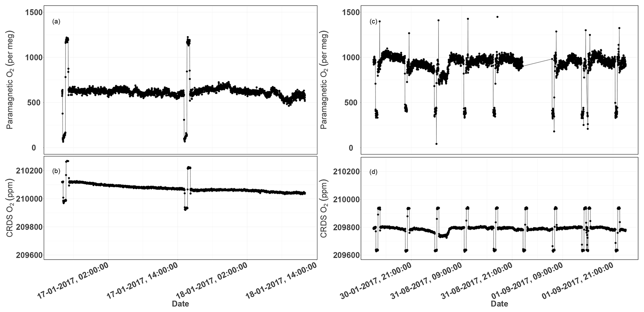
Figure 13Parallel ambient air measurements from the paramagnetic and CRDS analyzers at the beginning of the testing period (a, b, January 2017) and the second phase of testing (c, d, September 2017). The spikes are measurements from the two standard gases bracketing the ambient air values.
Figure 13a and b show the 1 min average ambient air measurements from the rooftop inlet from the paramagnetic and CRDS analyzers at the beginning of the testing period, including standard gases measured every 12 h. While the paramagnetic analyzer seemed to be stable, the CRDS analyzer showed a strong drift for an extended period. This could be due to unstable conditions in the CRDS measurement system as it started operating right after it was unpacked. Hence, we examined the temperature inside the instrument chassis and pressure records, which were stable within the manufacturer's recommended range during this period. As the CRDS analyzer incorporates a water correction function, interference from this species should be well accounted for. Even when comparing the analyzer's parallel water measurements to water measurements from the NDIR system, such a drift was not observed. It should be noted that the two internal standard gases, which were less frequently measured (every 12 h) during this period, were also drifting following similar pattern. This implies that the drift is associated with the analyzer. Interestingly, this pattern can be modeled using a polynomial function which can then be used to correct for the observed drift in the ambient air measurements. After applying a polynomial drift correction, we were able to fully account for the observed drift. However, the manufacturer decided to further investigate possible causes of this drift. After further improvements, we obtained the first commercial analyzer in September 2017 and repeated the above tests (Fig. 13c, d). The abovementioned drift was no longer observed in the standard gases nor in ambient air measurements.
We believe that the optical amplifier that caused the drift in the first system – and is no longer included in the design of the product – produced a significant amount of broadband light that could have filled the cavity (albeit with a low coupling coefficient), and would have caused the instrument to ring-down with a different (and generally much faster) time constant to that of the baseline loss of the cavity. However, the ring-down time on the peak of the oxygen line is just 10 microseconds, such that the broadband light might have distorted the single exponential decay of the central laser frequency, leading to the observed drift in the oxygen signal. However, we were not able to confirm this hypothesis.
3.2.3 Water correction test
Measurements of oxygen are reported as both wet (O2,raw) and dry (O2,dry) mole fractions by the CRDS analyzer, as it also measures water vapor in parallel at its water absorption line (7817 cm−1) and corrects for the dilution effect based on a built-in numerical function:
where H2O is the measured water mole fraction.
The efficiency of the water correction by this function was assessed in two ways: (i) by comparing the water vapor content in standard air measured by this analyzer with similar measurements from the NDIR analyzer and (ii) by comparing the oxygen mixing ratios between non-dried ambient air measured and corrected for water dilution from the CRDS analyzer with dried air measured using a paramagnetic analyzer.

Figure 14Parallel water vapor measurements for a dried ambient air from both the NDIR and CRDS analyzers. Note that the water values from the NDIR analyzer are not calibrated.
Figure 14 shows the water vapor content for standard gases measured continuously for 2 d by the CRDS and NDIR analyzers. Note that the two data sets are manually fitted to each other, as the measured water values from the NDIR analyzer are not calibrated. Based on this plot, the two analyzers are in very good agreement, although there are small differences during very dry conditions (low water content).
Figure 15a shows the dried ambient air water measurements from both analyzers, with frequent spikes due to valve switching while measuring standard gases. In the second case, where the water trap was bypassed and non-dried air was allowed to the CRDS analyzer while the dried air flow to the NDIR was maintained (Fig. 15b), a clear increase in the water measurements in the CRDS analyzer can be observed. Here, it should be noted that there are no spikes in the water measurements of the CRDS analyzers, as there are no standard gas measurements in between and the inlet is directly connected to the CRDS analyzer (Fig. 11). Figure 15c and d show the difference in the oxygen measurements of ambient air measured using both analyzers in the two abovementioned cases (note that the CRDS uses its built-in water correction function and applies Eq. 5). The measurements of the paramagnetic analyzer were scaled to parts per million by applying the correlation equation obtained from the six standard gas measurements of the two analyzers (Fig. A1). Note that the CRDS measurements were corrected for the observed drift using the polynomial fit of the two standard gas measurements stated above.
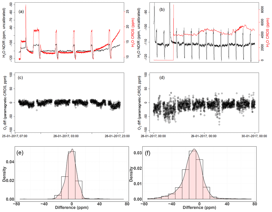
Figure 15Results of water correction tests. Water measurements of the NDIR (left axis) for dry conditions (a, b) and the CRDS analyzer (right axis) for dry (a) and wet (b) conditions. The difference in oxygen measurements between the paramagnetic and the CRDS instrument using the built-in water correction for the CRDS values under dry (c) and wet (d) conditions. Panels (e) and (f) show the population density functions.
In the first period of the measurement when both analyzers measured dried ambient air, the absolute differences between the 1 min averages measured over 2 d by the two analyzers were mostly within 15 ppm (Fig. 15c) and were symmetrically distributed around zero (Fig. 15e). However, when wet air was admitted to the CRDS analyzer and the built-in water correction was applied, a stronger variability was observed in the calculated differences (Fig. 15d). This implies stronger short-term variability in the CRDS analyzer measurement values (as nothing was changed for the paramagnetic measurement system) when wet samples are analyzed. The more negative values in the differences (Fig. 15f) can also be associated with an overestimation of the O2 mixing ratios by the CRDS, originating from an overestimated water correction. However, detailed evaluation of the analyzer's water correction function is beyond the scope of this study.
3.3 Field Measurements
After a series of tests at University of Bern, we conducted multiple field measurements at the high-altitude research station Jungfraujoch and the Beromünster tall tower sites in Switzerland described below.
3.3.1 Tests at the high-altitude research station Jungfraujoch
The high-alpine research station Jungfraujoch is located on the northern ridge of the Swiss Alps (46∘33′ N, 7∘59′ E) at an elevation of 3580 m a.s.l. It is one of the Global Atmosphere Watch (GAW) stations and is well-equipped for measurements of numerous species and aerosols. The site is above the planetary boundary layer most of the time due to its high elevation (Henne et al., 2010; Zellweger et al., 2003). However, thermally uplifted air from the surrounding valleys during hot summer days or polluted air from heavily industrialized northern Italy may reach this site (Zellweger et al., 2003). The Division of Climate and Environmental Physics at the University of Bern has been monitoring CO2 and O2 mixing ratios at this site based on weekly flask sampling and continuous measurements since 2000 and 2004, respectively (Schibig et al., 2015). The CO2 mixing ratio is measured using a commercial NDIR analyzer (S710 UNOR, SICK MAIHAK), whereas O2 is measured using a paramagnetic sensor (PM1155 oxygen transducer, Servomex Ltd, UK) and fuel cells (Max-250, Maxtec, USA) installed inside a custom-built controlling unit. Similar to the comparison tests at the University of Bern, we conducted parallel measurements between the CRDS analyzer and the paramagnetic cell at this high-altitude site from 3 to 14 February 2017. The measurement of ambient air in the Jungfraujoch system is composed of sequential switching between low-span (LS) and high-span (HS) calibration gases followed by a target gas (T) measurement (once a day) to evaluate the overall system performance and finally a working gas (WG) measurement before switching back to ambient air.
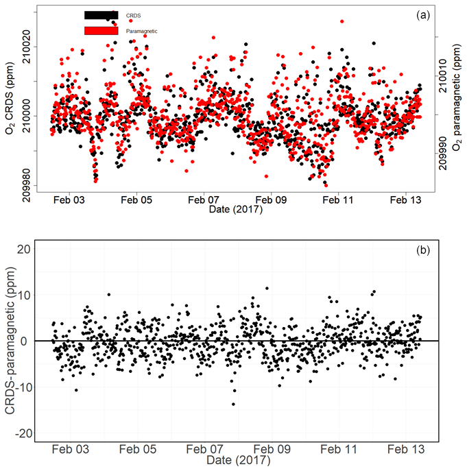
Figure 16Calibrated ambient air oxygen measurements (1 min average) at the Jungfraujoch site using the CRDS and paramagnetic analyzers (both in parts per million) (a) and the absolute difference between the two measurements (in parts per million) (b) carried out by matching time stamps.
Figure 16a shows the calibrated 1 min averaged O2 mixing ratios measured at this high-altitude site in comparison with the paramagnetic oxygen analyzer already available at the site. Despite the strong variability observed during the 10 d measurement period for both analyzers, very good agreement was observed between them.
Figure 16b shows the absolute difference of 1 min averages in atmospheric O2 measured at Jungfraujoch between the two analyzers, which are mostly within ±5 ppm range (but are sometimes as high as ±10 ppm) without an offset. However, for generally reported 10 min, 30 min, or 1 h means these values correspond to < 1.5, < 1, and < 0.65 ppm, respectively.
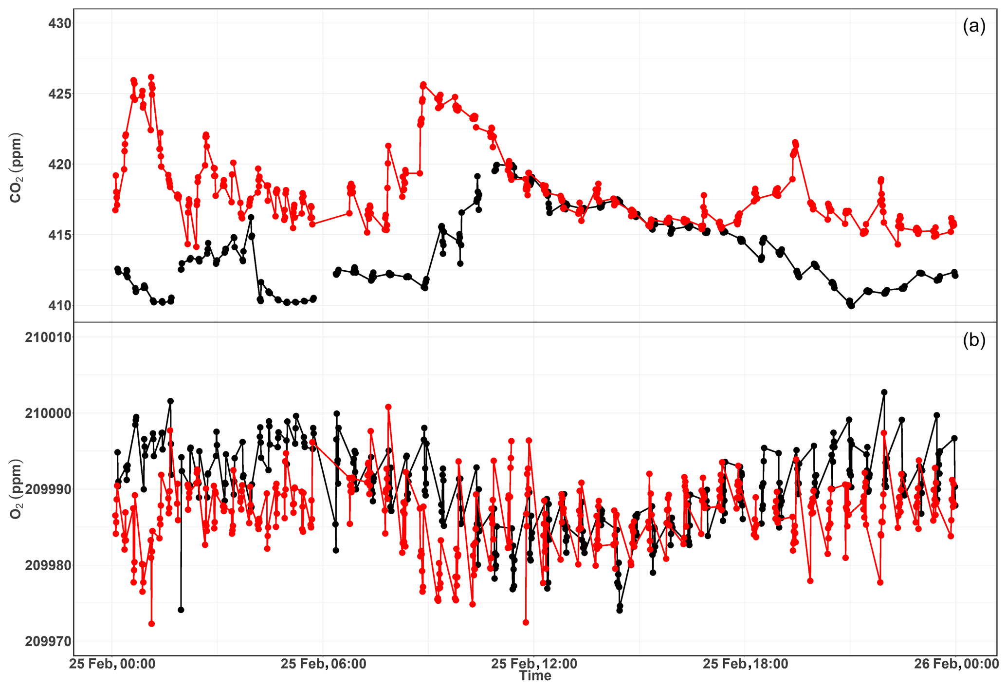
Figure 17Diurnal variations of CO2 (a) and O2 (b) measurements from the 12 m (red) and the 212.5 m (black) height levels at Beromünster tower.
3.3.2 Tests at the Beromünster tall tower site
The Beromünster tower is located near the southern border of the Swiss Plateau, which is the comparatively flat part of Switzerland between the Alps in the south and the Jura Mountains in the northwest (47∘11′23′′ N, 8∘10′32′′ E, 797 m a.s.l.); this region is characterized by intense agriculture and a rather high population density. A detailed description of the tower measurement system as well as a characterization of the site with respect to local meteorological conditions, seasonal and diurnal variations of greenhouse gases, and regional representativeness can be obtained from previous publications (Berhanu et al., 2016, 2017; Oney et al., 2015; Satar et al., 2016). The tower is 217.5 m tall with access to five sampling heights (12.5, 44.6, 71.5, 131.6, and 212.5 m) for the measurement of CO, CO2, CH4, and H2O using cavity ring-down spectroscopy (Picarro Inc., G2401). By sequentially switching from the highest to the lowest level, mixing ratios of these trace gases were recorded continuously for 3 min per height, but only the last 60 s were retained for data analysis. The calibration procedure for ambient air includes measurements of reference gases with high and low mixing ratios that are traceable to international standards (WMO-X2007 for CO2 and WMO-X2004 for CO and CH4), as well as target gas and more frequent working gas determinations to ensure the quality of the measurement system. From 2 years of data, a long-term reproducibility of 2.79 ppb, 0.05 ppm, and 0.29 ppb for CO, CO2 and CH4, respectively, was determined for this system (Berhanu et al., 2016).
Between 15 February and 2 March 2017, we connected the new CRDS oxygen analyzer in series with the CO2 analyzer (Picarro G2401) and measured the O2 mixing ratios at the corresponding heights. Similar to the CO2 measurements, O2 was also measured for 3 min at each height. During this period, we evaluated the two features (isotopic mode and concentration mode) of the CRDS analyzer. In the isotopic mode, the CRDS measured the δ18O values as well as the O2 concentration, whereas in concentration mode only the latter was measured.
During the tests conducted at this tower site, we first evaluated the two operational modes (concentration versus isotopic modes) of the CRDS analyzer. Ambient air measurements in isotopic mode over a 4 d period showed a strong variability in the measured oxygen mixing ratios and it was not possible to distinguish the variability in the O2 mixing ratios among the five height levels. The calculated 1 min standard error for ambient air measurements was as high as 10 ppm, whereas a standard error of less than 1 ppm was determined from similar measurements in the concentration mode. Additionally, comparing the O2 values between the two modes, frequent short-term variation in ambient air O2 (∼200 ppm) was observed in the isotope mode measurements, whereas the variation in the concentration mode was significantly smaller (∼30 ppm). This precision degradation is due to the weaker 16O oxygen line used for the isotopic mode, and the fact that far more ring-downs are collected on the rare isotopologue in isotopic mode. Hence, we conducted the remaining test measurements in concentration mode.
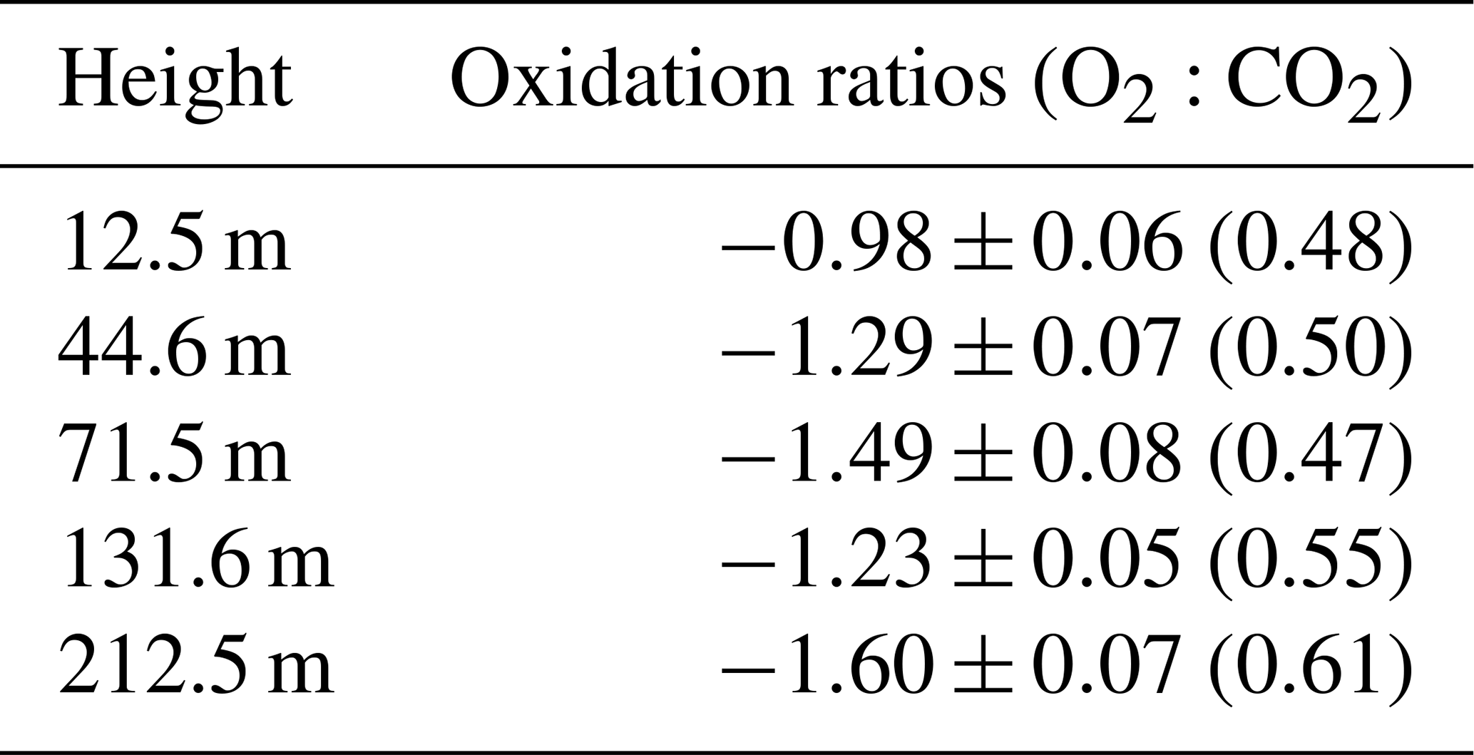
As this tower has five sampling height levels, we first undertook 3 min of switching per inlet level, which enabled four measurements per hour at a given level. However, we noticed hardly any difference among the different levels due to strong short-term variability in O2 mixing ratios between the consecutive heights. Hence, we switched to a longer sampling period of 6 min per height. Figure 17 shows the diurnal CO2 and O2 variations at the lowest (12 m) and highest (212.5 m) sampling heights of the tower. These two heights were selected in order to better illustrate the difference in the mixing ratios. The CO2 mixing ratios in Fig. 17a show higher values at the 12 m inlet than at the highest level most of the day, due to the former level's proximity to sources, except during the afternoon (11:00–17:00 UTC) when both levels show similar but decreasing CO2 mixing ratios. This was due to the presence of a well-mixed planetary boundary layer (PBL; Satar et al., 2016). The lag in the CO2 peak between the two height levels of about 2 h indicates the duration for uniform vertical mixing along the tower during winter 2017. The opposite variability patterns are also clearly visible in the O2 mixing ratios shown in Fig. 17b with a clear distinction between the two height levels during early in the morning and in the evening, whereas similar O2 values were observed in the afternoon. These opposing profiles are expected, as CO2 and O2 are linearly coupled with a mean oxidation ratio of (Severinghaus, 1995) for land biospheric processes (photosynthesis and respiration) and for fossil fuel burning (Keeling, 1988b).
Table 2 shows the oxidation ratios derived as the slopes of the linear regression between CO2 and O2 mixing ratios at the different height levels measured on 25 February 2017. Accordingly, height-dependent slopes were observed with a slope of at the lowest level, close to the biological-process-induced slope but slightly lower than its mean value. For the highest level, we calculated a slope of – a value close to the fossil fuel combustion oxidation ratio. Note that, depending on the fossil fuel type, the oxidation ratio can range between −1.17 and −1.95 for coal and natural gas, respectively (Keeling, 1988b). While the slopes derived for the two other levels (44.6 and 131.6 m) show similar values between the highest and lowest height levels, possibly from mixed sources, the middle level showed a slightly higher slope than these two levels but was still within the large range between the lowest and highest inlet heights.
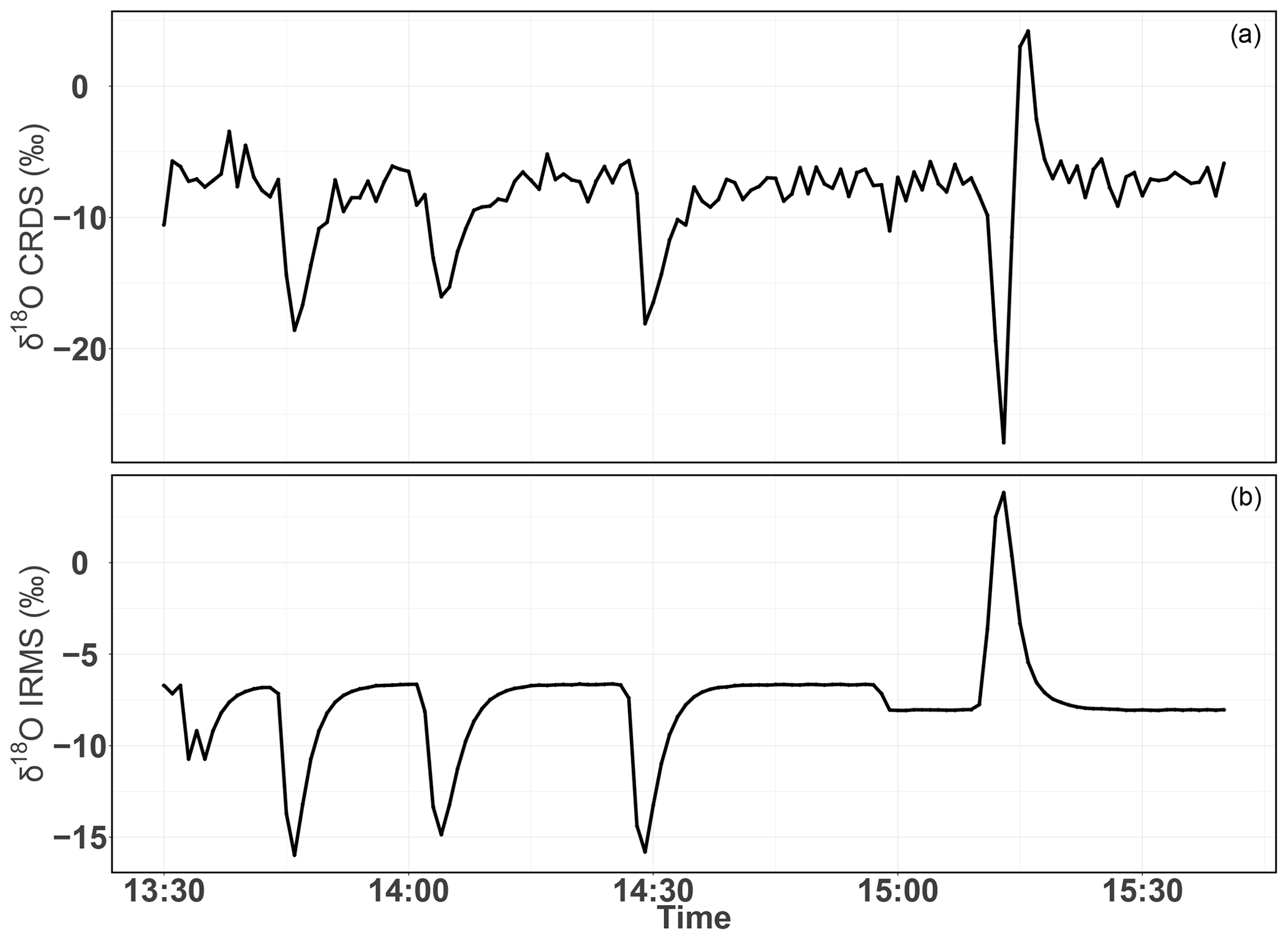
Figure 18Consecutive δ18O measurements of a standard gas (CO2-free air) filled into three flasks followed by measurement of breath air using the CRDS analyzer (a) and the IRMS (b). These measurements were carried out in the middle of ambient air measurements.
Table 2The CO2 and O2 correlation coefficients at the different height levels derived using the least-squares fit and the correlation coefficients (r2). Uncertainties are calculated as the standard error of the slope.
3.4 Evaluation of the δ18O measurements
To further evaluate the analyzer's performance with respect to measuring stable oxygen isotopes, we conducted ambient air isotopic composition measurements as well as analyzing a standard gas without CO2, which had a known δ18O value. The choice of this CO2-free air standard gas is twofold: one it has a known δ18O value and second as it has no interference from a possible CO2 absorption band overlap. For this test three 0.5 L glass flasks were preconditioned and filled with this standard gas to ambient pressure. These flasks were attached before or after the water trap (Fig. 11) and measured in a similar fashion to ambient air measurements. These measurements were then compared with δ(34O∕32O) values obtained by parallel measurements using the IRMS.
Figure 18 shows the δ18O values of ambient air from the roof top with three consecutive measurements of glass flasks filled with CO2-free air in-between followed by a fourth flask filled with breath air. Excellent agreement was observed for measurements from both instruments for the three flasks filled with a standard gas. However, the fourth flask with breath air showed a signal opposite to that of the IRMS measurements. As breath air contains large amount of water and CO2 in addition to O2, which can possibly interfere with the CRDS analyzer measurements, we removed H2O and CO2 using a cryogenic trap (−130 ∘C); in an additional experiment, we also used Schütze reagent to remove both CO and CO2. However, we did not observe any improvement towards an agreement with the IRMS measurements. Therefore, another gas component in the breath air must be responsible for the abovementioned interference. Based on the absorption lines in the spectral range of the instrument (7878 cm−1) retrieved from the HITRAN database, we expect the interference to stem from either carbon monoxide (now excluded by the tests), methane, or volatile organic compounds including acetone, ethanol, methanol, or isoprenes – all of which have been measured in breath air (Gao et al., 2017; Gottlieb et al., 2017; Mckay et al., 1985; Ryter and Choi, 2013; Wolf et al., 2017). Further investigations are required to shed light on these interferences in order to take corresponding action to surpass these shortcomings in the isotope analysis based on cavity ring-down spectroscopy.
We thoroughly evaluated the performance of a new CRDS analyzer that measures O2 mixing ratios and isotopic composition using both laboratory and field tests. Even if a drift in the analyzer was observed at the beginning of this study, which could be easily corrected by calibration, the recent analyzers built by the manufacturer have not shown any such instrumental drift. However, prior tests are recommended to assess the analyzer's stability.
The tee-junction tests for the current measurement setup based on the measurements of two standard gases showed a difference within the measurement uncertainty. However, this effect may become significant when applying larger splitting ratios, and we recommend conducting further experiments to accurately quantify this influence for larger splitting ratios.
We observed a strong influence of dilution in the measured O2 values in the presence of high CO2 mixing ratios. Even if such an influence may not be critical for the present study, such an effect might be significant in other studies where higher CO2 mixing ratios might be present; thus, we recommend following a correction strategy based on parallel CO2 measurements. This also applies for more accurate analysis.
The water correction applied by the instrument's built-in function seems to sufficiently correct for the water vapor influence. However, a larger variability of the difference was observed between the CRDS analyzer and the paramagnetic cell when dried samples were used in both systems. This may possibly be due to an overcorrection by the water correction function of the CRDS analyzer when dried samples were used. This is particularly true for the very low water vapor range (< 100 ppm). We believe that it is important to further investigate this issue and identify an improved water correction strategy.
Based on the analysis of O2 mixing ratios in the concentration and isotopic modes, we observed a significant decrease in precision (about 10-fold) in the latter measurement mode. The measured δ18O values for the standard air by the CRDS analyzer are in excellent agreement with the IRMS values. However, such measurements for breath air showed a contrasting signal, possibly due to interference from other gases such as CH4. Hence, we recommend further investigation on such possible contaminants and how to possibly remove them while conducting ambient air measurements. However, we believe that this analyzer can be used for tracer experiments where artificially enriched isotopes are used to study biological processes, such as photosynthesis in plants, using isotopically labeled CO2 and H2O.
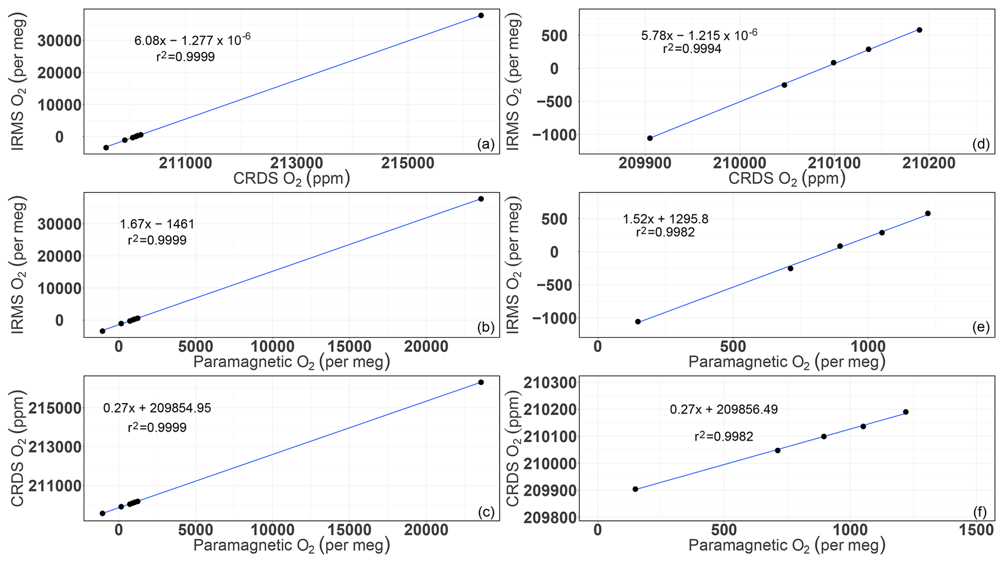
Figure A1Correlations of the O2 mixing ratios measured by the CRDS and paramagnetic analyzers with the mass spectrometric measurements (uncalibrated values). Panels (a), (b), and (c) are for all of the cylinders measured (standards 1 to 8), whereas panels (d), (e), and (f) are after selecting standards 1–5.
Table A1Different dilution scenarios and their effect on air-like compositions.
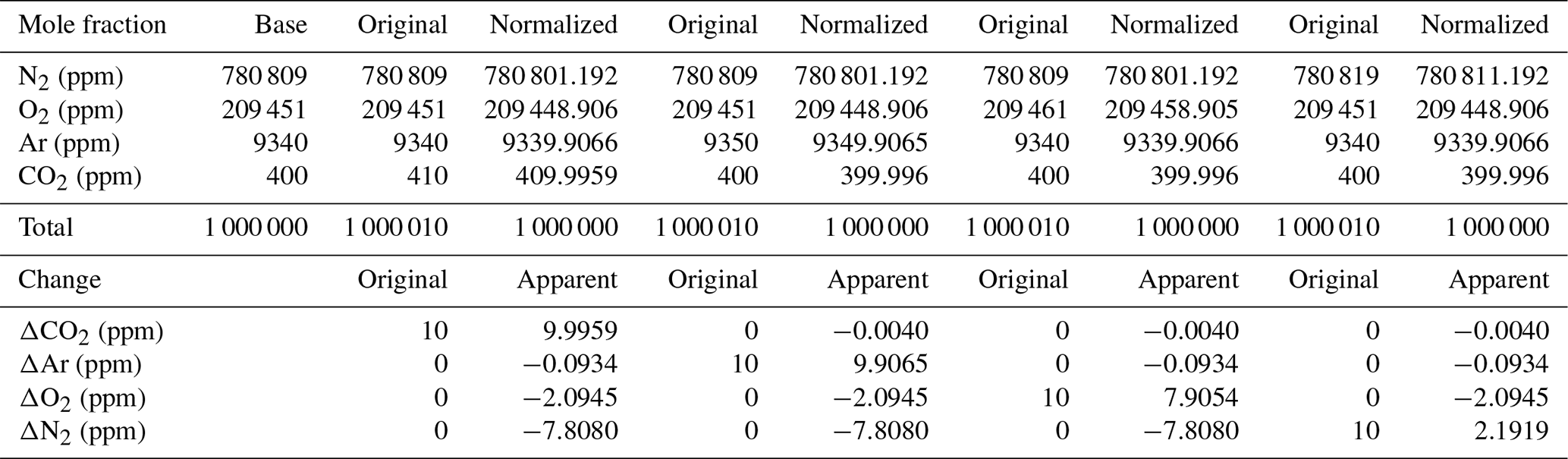
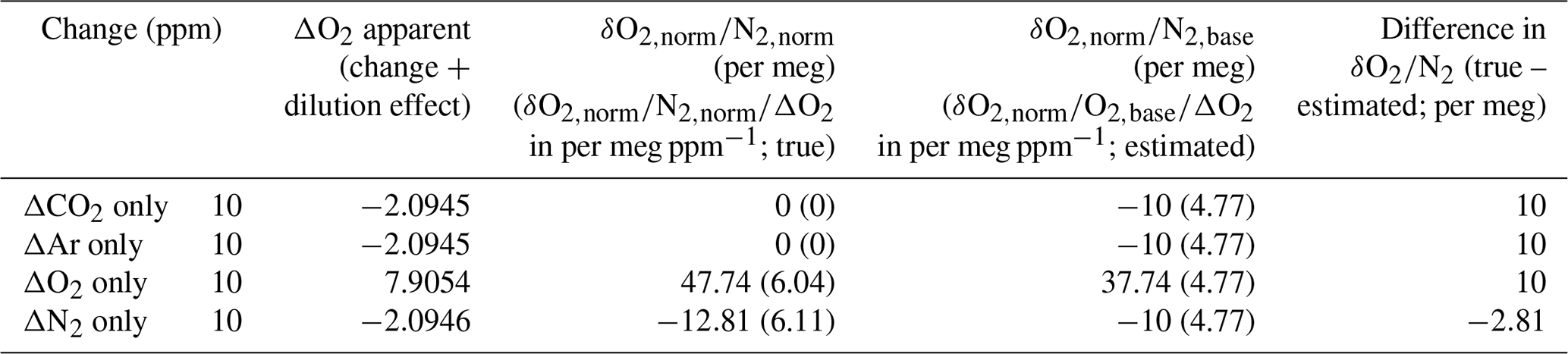
Table A2Mole fraction to delta conversion for air-like compositions according to different scenarios.
Generally, the delta notation (δ(O2∕N2)), as given in Eq. (1) of this publication (and also shown below), is used in order to circumvent the influences of dilution by other gas components when determining oxygen mole fractions (Table A1). However, several instruments are used to measure the oxygen mole fraction, such as the paramagnetic cell, the UV cell, and the CRDS analyzer presented here. Therefore, thorough consideration of the conversion from parts per million (mole fraction) to per meg (δ(O2∕N2) notation) is necessary and is consequently explained in the following.
Following Eq. (1) in Thojima et al. (2000), the per meg to parts per million conversion has a slope of 6.04 if a change in oxygen alone is applied, as seen in Table A2. It changes slightly to 6.11 per meg ppm−1, when we consider nitrogen changes only, or to a slope of zero (horizontal line) when talking about any other changes in air components excluding oxygen and nitrogen. The fact that our supplementary plot shows slopes of 5.78 (for the first five standards) or 6.08 per meg ppm−1 (for all standards except standard 7, ST-7) is due to the mixed influence of dilution effects. The lower slope of 5.78 per meg ppm−1 particularly documents the influence of the CO2 dilution effect.
Note that under the assumption that the atmospheric N2 content is constant (i.e., N2sample equals N2reference), we convert relative changes in oxygen given in per meg to oxygen changes in parts per million (equivalent to micromol mol−1) by multiplying by the O2 mole fraction (O2reference) expressed as 209 500 ppm (the O2 mole fraction of atmospheric air) (Machta and Hughes, 1970). Hence 1 ppm corresponds to approximately 4.8 per meg, or 1 per meg to 1∕4.8 (209 500/106) ppm.
This is used in our approach, as the Picarro instrument measures the O2 mole fraction which then requires conversion to an O2∕N2 ratio. The effect of water dilution (the amount of water vapor is measured by the CRDS instrument) is taken into account as described in the main body of the paper. However, no other dilution effect is considered unless additional information is available, e.g., CO2 concentration measurements. Indeed these dilution effects can be significant, and are displayed in Table A2.
This will lead to the following changes for oxygen, the true and estimated (when N2 is not measured) δ(O2∕N2) ratios, and the difference in these δ(O2∕N2) values: is calculated (e.g., Thojima et al., 2000) or measured, for instance, by mass spectrometry; uses a fixed conversion factor of 4.77 per meg ppm−1 based on the measured O2 mole fraction (ppm), for instance, by the CRDS analyzer.
Incorrectly assumed N2, Ar, CO2, or any additional gas component can lead to changes in the estimated values, as stated in the Table A2. For example, a 10 ppm increase in CO2 can lead to a bias of −10 per meg in compared with the true value. This is simply the dilution effect that the increased CO2 concentration has on the corresponding O2 mole fraction (Table A1; the dilution in oxygen corresponds to the percentage-wise assignment of the excess CO2 in parts per million to oxygen, i.e., −10 ppm x oxygen mole fraction =2.0946 ppm, if the O2 mole fraction corresponds to 0.20946). As can be seen from Table A2, the addition of 10 ppm N2 leads to a reduced and inverse effect for the difference in δO2∕N2 (true – estimated) because the dilution effect on O2 cannot compensate for the change from the increase in nitrogen; therefore, it scales with −10 ppm x (oxygen mole fraction/nitrogen mole fraction). This also shows that the difference in the delta values (true – estimated) scales with the δO2∕N2 ratio present in the sample. Therefore, the best results are obtained when the calibration gases for which the gas composition is known have a composition that is close to the sample gas composition. In our case, this is given – but can certainly be improved – as we are comparing natural air to an air standard. Yet, determinations of the standards that have been used in this study have a range of N2 concentrations from −110 to +110 ppm for ST-1 to ST-5, whereas ST-6 (+700 ppm) and ST-8 (−6200 ppm) are significantly different from the primary standard used for mass spectrometric determination in this study. Therefore, special attention is required for the precise determination of the standard gas composition and the control of the air sample composition by means of flask measurements in order to detect potential fractionation effects during air intake.
The data are available upon request from the University of Bern (leuenberger@climate.unibe.ch).
TAB, ML, and PN carried out the measurements at the field sites and at the University of Bern laboratory. JH, CR, and DK were involved in the instrument development and performed tests at the Picarro company site. TAB and ML wrote a first draft of the paper, and JH and CR provided input on the instrument development section of the paper. All authors were involved in editing the paper.
The authors declare that they have no conflict of interest.
We would like to thank ICOS-RI and the Swiss National Science Foundation (SNF) for funding ICOS-CH (grant nos. 20FI21_148994 and 20FI21_148992). We are also grateful to the International Foundation High Alpine Research Stations, Jungfraujoch and Gornergrat. The measurement system at the Beromünster tower was built and maintained by the CarboCount-CH (grant no. CRSII2_136273) and IsoCEP (grant no. 200020_172550) projects which are both funded by SNF.
This research has been supported by the Swiss National Science Foundation (SNF) through its funding for the ICOS-CH (grant nos. 20FI21_148994 and 20FI21_148992), CarboCount-CH (grant no. CRSII2_136273), and IsoCEP (grant no. 200020_172550) projects.
This paper was edited by Christof Janssen and reviewed by two anonymous referees.
Battle, M., Bender, M. L., Tans, P. P., White, J. W. C., Ellis, J. T., Conway, T., and Francey, R. J.: Global carbon sinks and their variability inferred from atmospheric O-2 and delta C-13, Science, 287, 2467–2470, 2000.
Bender, M. L., Tans, P. P., Ellis, J. T., Orchardo, J., and Habfast, K.: A High-Precision Isotope Ratio Mass-Spectrometry Method for Measuring the O-2 N-2 Ratio of Air, Geochim. Cosmochim. Ac., 58, 4751–4758, 1994.
Berhanu, T. A., Satar, E., Schanda, R., Nyfeler, P., Moret, H., Brunner, D., Oney, B., and Leuenberger, M.: Measurements of greenhouse gases at Beromünster tall-tower station in Switzerland, Atmos. Meas. Tech., 9, 2603–2614, https://doi.org/10.5194/amt-9-2603-2016, 2016.
Berhanu, T. A., Szidat, S., Brunner, D., Satar, E., Schanda, R., Nyfeler, P., Battaglia, M., Steinbacher, M., Hammer, S., and Leuenberger, M.: Estimation of the fossil fuel component in atmospheric CO2 based on radiocarbon measurements at the Beromünster tall tower, Switzerland, Atmos. Chem. Phys., 17, 10753–10766, https://doi.org/10.5194/acp-17-10753-2017, 2017.
Crosson, E. R.: A cavity ring-down analyzer for measuring atmospheric levels of methane, carbon dioxide, and water vapor, Appl. Phys. B, 92, 403–408, https://doi.org/10.1007/s00340-008-3135-y, 2008.
Filges, A., Gerbig, C., Rella, C. W., Hoffnagle, J., Smit, H., Krämer, M., Spelten, N., Rolf, C., Bozóki, Z., Buchholz, B., and Ebert, V.: Evaluation of the IAGOS-Core GHG package H2O measurements during the DENCHAR airborne inter-comparison campaign in 2011, Atmos. Meas. Tech., 11, 5279–5297, https://doi.org/10.5194/amt-11-5279-2018, 2018.
Gao, F., Zhang, X., Zhang, X., Wang, M., and Wang, P.: Virtual electronic nose with diagnosis model for the detection of hydrogen and methane in breath from gastrointestinal bacteria, 28–31 May 2017, 1–3, https://doi.org/10.1109/ISOEN.2017.7968880, 2017.
Gordon, E., Rothman, S., Hill, C., Kochanov, V., Tan, Y., Bernath, P., Birk, M., Boudon, V., Campargue, A., Chance, K., Drouin, J., Flaud, J., Gamache, R. R., Hodges, J., Jacquemart, D., Perevalov, I., Perrin, A., Shine, P., Smith, M., Tennyson, J., Toon, G., Tran, H., Tyuterev, G., Barbe, A., Császár, G., Devi, M., Furtenbacher, T., Harrison, J., Hartmann, J., Jolly, A., Johnson, J., Karman, T., Kleiner, I., Kyuberis, A. A., Loos, J., Lyulin, M., Massie, S., Mikhailenko, S., Moazzen-Ahmadi, N., Muller, S., Naumenko, O. V., Nikitin, A. V., Polyansky, O. L., Rey, M., Rotger, M., Sharpe, S., Sung, K., Starikova, E., Tashkun, S., Auwera, J., Wagner, G., Wilzewski, J., Wcisło, P., Yu, S., and Zak, E. J.: The HITRAN2016 molecular spectroscopic database, Science Direct, 203, 3–69, 2017.
Goto, D., Morimoto, S., Ishidoya, S., Aoki, S., and Nakazawa, T.: Terrestrial biospheric and oceanic CO2 uptake estimated from long-term measurements of atmospheric CO2 mole fraction, δ13C and δ(O2∕N2) at Ny-Ålesund, Svalbard, J. Geophys. Res.-Biogeo., 122, https://doi.org/10.1002/2017JG003845, 2017.
Gottlieb, K., Le, C. X., Wacher, V., Sliman, J., Cruz, C., Porter, T., and Carter, S.: Selection of a cut-off for high- and low-methane producers using a spot-methane breath test: results from a large north American dataset of hydrogen, methane and carbon dioxide measurements in breath, Gastroenterol. Rep., 5, 193–199, 2017.
Hartmann, J.-M., Boulet, C., and Robert, D.: Collisional Effects on Molecular Spectra, Elsevier Science, 2008.
Henne, S., Brunner, D., Folini, D., Solberg, S., Klausen, J., and Buchmann, B.: Assessment of parameters describing representativeness of air quality in-situ measurement sites, Atmos. Chem. Phys., 10, 3561–3581, https://doi.org/10.5194/acp-10-3561-2010, 2010.
Hodges, J. T., Layer, H. P., Miller, W. W., and Scace, G. E.: Frequency-stabilized single-mode cavity ring-down apparatus for high-resolution absorption spectroscopy, Rev. Sci. Instrum. 75, 849–863, https://doi.org/10.1063/1.1666984, 2004.
Keeling, R. F.: Development of an Interferometric Oxygen Analyzer for Precise Measurement of the Atmospheric O2 Mole Fraction, UMI, available at: http://bluemoon.ucsd.edu/publications/ralph/34_PhDthesis.pdf (last access: 18 December 2019), 1988a.
Keeling, R. F.: Measuring correlations between atmospheric oxygen and carbon dioxide mole fractions: A preliminary study in urban air, J. Atmos. Chem., 7, 153–176, 1988b.
Keeling, R. F. and Manning, A. C.: 5.15 – Studies of Recent Changes in Atmospheric O2 Content A2 – Holland, Heinrich D., in: Treatise on Geochemistry (Second Edition), edited by: Turekian, K. K., Elsevier, Oxford, 2014.
Keeling, R. F. and Shertz, S. R.: Seasonal and Interannual Variations in Atmospheric Oxygen and Implications for the Global Carbon-Cycle, Nature, 358, 723–727, 1992.
Keeling, R. F., Stephens, B. B., Najjar, R. G., Doney, S. C., Archer, D., and Heimann, M.: Seasonal variations in the atmospheric O-2/N-2 ratio in relation to the kinetics of air-sea gas exchange, Global Biogeochem. Cy., 12, 141–163, 1998.
Lamouroux, J., Sironneau, V., Hodges, J. T., and Hartmann, J. M.: Isolated line shapes of molecular oxygen: Requantized classical molecular dynamics calculations versus measurements, Phys. Rev. A, 89, 042504, https://doi.org/10.1103/PhysRevA.89.042504, 2014.
Le Quéré, C., Andrew, R. M., Friedlingstein, P., Sitch, S., Pongratz, J., Manning, A. C., Korsbakken, J. I., Peters, G. P., Canadell, J. G., Jackson, R. B., Boden, T. A., Tans, P. P., Andrews, O. D., Arora, V. K., Bakker, D. C. E., Barbero, L., Becker, M., Betts, R. A., Bopp, L., Chevallier, F., Chini, L. P., Ciais, P., Cosca, C. E., Cross, J., Currie, K., Gasser, T., Harris, I., Hauck, J., Haverd, V., Houghton, R. A., Hunt, C. W., Hurtt, G., Ilyina, T., Jain, A. K., Kato, E., Kautz, M., Keeling, R. F., Klein Goldewijk, K., Körtzinger, A., Landschützer, P., Lefèvre, N., Lenton, A., Lienert, S., Lima, I., Lombardozzi, D., Metzl, N., Millero, F., Monteiro, P. M. S., Munro, D. R., Nabel, J. E. M. S., Nakaoka, S., Nojiri, Y., Padin, X. A., Peregon, A., Pfeil, B., Pierrot, D., Poulter, B., Rehder, G., Reimer, J., Rödenbeck, C., Schwinger, J., Séférian, R., Skjelvan, I., Stocker, B. D., Tian, H., Tilbrook, B., Tubiello, F. N., van der Laan-Luijkx, I. T., van der Werf, G. R., van Heuven, S., Viovy, N., Vuichard, N., Walker, A. P., Watson, A. J., Wiltshire, A. J., Zaehle, S., and Zhu, D.: Global Carbon Budget 2017, Earth Syst. Sci. Data, 10, 405–448, https://doi.org/10.5194/essd-10-405-2018, 2018.
Machta, L. and Hughes, E.: Atmospheric Oxygen in 1967 to 1970, Science, 168, 3939, 1582–1584, 1970.
Manning, A.: Temporal variability of atmospheric oxygen from both continuos and measurements and a flask sampling network: tools for studying the global carbon cycle, PhD, University of California, San Diego, San Diego, Calofornia, USA, 2001.
Manning, A. C. and Keeling, R. F.: Global oceanic and land biotic carbon sinks from the Scripps atmospheric oxygen flask sampling network, Tellus B, 58, 95–116, 2006.
Manning, A. C., Keeling, R. F., and Severinghaus, J. P.: Precise atmospheric oxygen measurements with a paramagnetic oxygen analyzer, Global Biogeochem. Cy., 13, 1107–1115, 1999.
Marrero, T. R. and Mason, E. A.: Gaseous Diffusion Coefficients, J. Phys. Chem. Ref. Data, 1, 3, https://doi.org/10.1063/1.3253094, 1972.
Martin, N. A., Ferracci, V., Cassidy, N., and Hoffnagle, J.: The application of a cavity ring-down spectrometer to measurements of ambient ammonia using traceable primary standard gas mixtures, Appl. Phys. B, 122, 219, https://doi.org/10.1007/s00340-016-6486-9, 2016.
Mckay, L. F., Eastwood, M. A., and Brydon, W. G.: Methane Excretion in Man – a Study of Breath, Flatus, and Feces, Gut, 26, 69–74, 1985.
Nevison, C. D., Keeling, R. F., Kahru, M., Manizza, M., Mitchell, B. G., and Cassar, N.: Estimating net community production in the Southern Ocean based on atmospheric potential oxygen and satellite ocean color data, Global Biogeochem. Cy., 26, https://doi.org/10.1029/2018GL079575, 2012.
Oney, B., Henne, S., Gruber, N., Leuenberger, M., Bamberger, I., Eugster, W., and Brunner, D.: The CarboCount CH sites: characterization of a dense greenhouse gas observation network, Atmos. Chem. Phys., 15, 11147–11164, https://doi.org/10.5194/acp-15-11147-2015, 2015.
Press, W. H., Teukolsky, S. A., Vetterling, W. T., and Flannery, B. P.: Numerical Recipes 3rd Edition: The Art of Scientific Computing, Cambridge Printing Press, Cambridge, England, 1986.
Press, W. H., Teukolsky, S. A., Vetterling, W. T., and Flannery, B. P.: Numerical recipes in C: the art of scientific computing, Cambridge University Press, London, 1992.
Ryter, S. W. and Choi, A. M. K.: Carbon monoxide in exhaled breath testing and therapeutics, J. Breath Res., 7, https://doi.org/10.1088/1752-7155/7/1/017111, 2013.
Satar, E., Berhanu, T. A., Brunner, D., Henne, S., and Leuenberger, M.: Continuous measurements (2012–2014) at Beromünster tall tower station in Switzerland, Biogeosciences, 13, 2623–2635, https://doi.org/10.5194/bg-13-2623-2016, 2016.
Schibig, M. F., Steinbacher, M., Buchmann, B., van der Laan-Luijkx, I. T., van der Laan, S., Ranjan, S., and Leuenberger, M. C.: Comparison of continuous in situ CO2 observations at Jungfraujoch using two different measurement techniques, Atmos. Meas. Tech., 8, 57–68, https://doi.org/10.5194/amt-8-57-2015, 2015.
Severinghaus, J. P.: Studies of the terresterial O2 and carbon cycles in sand dune gases and in Biosphere Doctoral PhD, Columbia University, New York, USA, 1995.
Steig, E. J., Gkinis, V., Schauer, A. J., Schoenemann, S. W., Samek, K., Hoffnagle, J., Dennis, K. J., and Tan, S. M.: Calibrated high-precision 17O-excess measurements using cavity ring-down spectroscopy with laser-current-tuned cavity resonance, Atmos. Meas. Tech., 7, 2421–2435, https://doi.org/10.5194/amt-7-2421-2014, 2014.
Stephens, B. B., Bakwin, P. S., Tans, P. P., Teclaw, R. M., and Baumann, D. D.: Application of a differential fuel-cell analyzer for measuring atmospheric oxygen variations, J. Atmos. Ocean. Tech., 24, 82–94, 2007.
Sturm, P., Leuenberger, M., Valentino, F. L., Lehmann, B., and Ihly, B.: Measurements of CO2, its stable isotopes, O2∕N2, and 222Rn at Bern, Switzerland, Atmos. Chem. Phys., 6, 1991–2004, https://doi.org/10.5194/acp-6-1991-2006, 2006.
Tan, Y., Kochanov, R. V., Rothman, L., and Gordon, I. E.: Introduction of Water‐Vapor Broadening Parameters and Their Temperature‐Dependent Exponents Into the HITRAN Database: Part I – CO2, N2O, CO, CH4, O2, NH3, and H2S, J. Geophys. Res.-Atmos., https://doi.org/10.1029/2019JD030929, 2019.
Tennyson, J., Bernath, P. F., Campargue, A., Császár, A. G., Daumont, L., Gamache, R. R., Hodges, J. T., Lisak, D., Naumenko, O. V., Rothman, L. S., Tran, H., Zobov, N. F., Buldyreva, J., Boone, C. D., De Vizia, M. D., Gianfrani, L., Hartmann, J.-M., McPheat, R., Weidmann, D., Murray, J., Ngo, N. H., and Polyansky, O. L.: Recommended isolated-line profile for representing high-resolution spectroscopic transitions, IUPAC Technical Report, 86, 1931–1943, 2014.
Tohjima, Y.: Method for measuring changes in the atmospheric O-2/N-2 ratio by a gas chromatograph equipped with a thermal conductivity detector, J. Geophys. Res.-Atmos., 105, 14575–14584, 2000.
Tran, H., Turbet, M., Hanoufa, S., Landsheere, X., Chelin, P., Ma, Q., and Hartmann, J.: The CO2–broadened H2O continuum in the 100–1500 cm−1 region: Measurements, predictions and empirical model, J. Quant. Spectrosc. Ra., 230, 75–80, 2019.
Valentino, F. L., Leuenberger, M., Uglietti, C., and Sturm, P.: Measurements and trend analysis of O2, CO2 and δ13C of CO2 from the high altitude research station Junfgraujoch, Switzerland – A comparison with the observations from the remote site Puy de Dôme, France, Sci. Total Environ., 391, 203–210, 2008.
Varghese, P. L. and Hanson, R. K.: Collisional narrowing effects on spectral line shapes measured at high resolution, Appl. Optics, 23, 2376–2385, 1984.
Wójtewicz, S., Cygan, A., Masłowski, P., Domysławska, J., Wcisło, P., Zaborowski, M., Lisak, D., Trawiński, R. S., and Ciuryło, R.: Spectral line-shapes of oxygen B-band transitions measured with cavity ring-down spectroscopy, J. Phys. Conf. Ser., 548, 012028, https://doi.org/10.1088/1742-6596/548/1/012028, 2014.
Wolf, P. G., Parthasarathy, G., Chen, J., O'Connor, H. M., Chia, N., Bharucha, A. E., and Gaskins, H. R.: Assessing the colonic microbiome, hydrogenogenic and hydrogenotrophic genes, transit and breath methane in constipation, Neurogastroent. Motil., 29, https://doi.org/10.1111/nmo.13056, 2017.
Zellweger, C., Forrer, J., Hofer, P., Nyeki, S., Schwarzenbach, B., Weingartner, E., Ammann, M., and Baltensperger, U.: Partitioning of reactive nitrogen (NOy) and dependence on meteorological conditions in the lower free troposphere, Atmos. Chem. Phys., 3, 779–796, https://doi.org/10.5194/acp-3-779-2003, 2003.
- Abstract
- Introduction
- Analyzer design principles
- Results and discussions
- Conclusions
- Appendix A
- Appendix B: Uncertainty consideration during mole fraction (ppm) to delta (per meg) conversion for air-like gas compositions according to different scenarios
- Data availability
- Author contributions
- Competing interests
- Acknowledgements
- Financial support
- Review statement
- References