the Creative Commons Attribution 4.0 License.
the Creative Commons Attribution 4.0 License.
 | 20 Dec 2019
Development of the DRoplet Ice Nuclei Counter Zurich (DRINCZ): validation and application to field-collected snow samples
Maria Cascajo-Castresana
Killian P. Brennan
Michael Rösch
Nora Els
Julia Werz
Vera Weichlinger
Lin S. Boynton
Sophie Bogler
Nadine Borduas-Dedekind
Claudia Marcolli
Ice formation in the atmosphere is important for regulating cloud lifetime, Earth's radiative balance and initiating precipitation. Due to the difference in the saturation vapor pressure over ice and water, in mixed-phase clouds (MPCs), ice will grow at the expense of supercooled cloud droplets. As such, MPCs, which contain both supercooled liquid and ice, are particularly susceptible to ice formation. However, measuring and quantifying the concentration of ice-nucleating particles (INPs) responsible for ice formation at temperatures associated with MPCs is challenging due to their very low concentrations in the atmosphere (∼1 in 105 at −30 ∘C). Atmospheric INP concentrations vary over several orders of magnitude at a single temperature and strongly increase as temperature approaches the homogeneous freezing threshold of water. To further quantify the INP concentration in nature and perform systematic laboratory studies to increase the understanding of the properties responsible for ice nucleation, a new drop-freezing instrument, the DRoplet Ice Nuclei Counter Zurich), is developed. The instrument is based on the design of previous drop-freezing assays and uses a USB camera to automatically detect freezing in a 96-well tray cooled in an ethanol chilled bath with a user-friendly and fully automated analysis procedure. Based on an in-depth characterization of DRINCZ, we develop a new method for quantifying and correcting temperature biases across drop-freezing assays. DRINCZ is further validated performing NX-illite experiments, which compare well with the literature. The temperature uncertainty in DRINCZ was determined to be ±0.9 ∘C. Furthermore, we demonstrate the applicability of DRINCZ by measuring and analyzing field-collected snow samples during an evolving synoptic situation in the Austrian Alps. The field samples fall within previously observed ranges for cumulative INP concentrations and show a dependence on air mass origin and upstream precipitation amount.
- Article
(11652 KB) - Full-text XML
- BibTeX
- EndNote


In the atmosphere, ice plays an important role in initiating precipitation and affects the radiative properties of clouds. As much as 80 % of land-falling precipitation initiates through the ice phase (Mülmenstädt et al., 2015), making it essential to understand the pathways for ice formation in the atmosphere. The ratio of cloud droplets to ice crystals in a mixed-phase cloud (MPC) alters the radiative properties of the cloud and its lifetime (Lohmann and Feichter, 2005; Matus and L'Ecuyer, 2017; Tan et al., 2016). This ratio is important for future climate projections, as warmer temperatures will lead to a decrease in ice content, ultimately increasing cloud lifetime and cloud albedo (Tan et al., 2016). Additionally, ice formation at temperatures above −38 ∘C in the atmosphere occurs primarily in MPCs through the freezing of cloud droplets (Ansmann et al., 2009; de Boer et al., 2011; Westbrook and Illingworth, 2011). Therefore, understanding ice formation in conditions associated with MPCs is of the utmost importance.
When an ice-nucleating particle (INP) gets immersed in a cloud droplet either by acting as a cloud condensation nucleus or through scavenging by a cloud droplet, the INP can induce ice formation by reducing the energy barrier associated with the formation of an ice germ and thus freeze at warmer temperatures than homogeneous freezing (Vali et al., 2015). To reproduce the immersion freezing pathway in the laboratory, several methods are used. Single-particle methods, such as continuous-flow diffusion chambers (Rogers, 1988; Stetzer et al., 2008) operated at water supersaturated conditions (DeMott et al., 2015, 2017; Hiranuma et al., 2015), or with extended chambers that activate individual particles into cloud droplets before exposing them to supercooled conditions (Burkert-Kohn et al., 2017; Kohn et al., 2016; Lüönd et al., 2010), allow for the quantification of the number concentration of INPs as a function temperature. Larger laboratory-based single-particle methods for examining INPs in the immersion mode include expansion chambers where cloud droplets are first formed by adiabatic cooling due to the expansion of an air volume (Niemand et al., 2012) or experiments where droplets are initially activated and then subsequently cooled as they travel through a laminar flow tube (Hartmann et al., 2011). Aerosols introduced into such systems by dry dispersion or atomization of suspensions and solutions allow for a range of particulates to be examined. However, the single-particle methods have detection limitations due to the background ice crystal concentration of the chamber and the optical methods for discriminating between ice and water. Due to the rarity of INPs at MPC conditions, single-particle methods are typically unable to quantify INP concentrations within natural ambient samples at temperatures higher than approximately −22 ∘C in remote regions without the use of concentrators (Cziczo et al., 2017).
In contrast bulk methods such as drop-freezing assays (Hill et al., 2014; Stopelli et al., 2014; Vali, 1971), differential scanning calorimetry (Kaufmann et al., 2016; Pinti et al., 2012) and microfluidic devices (Reicher et al., 2018; Riechers et al., 2013; Stan et al., 2009; Tarn et al., 2018) immerse the samples in water and can be used to detect lower atmospheric INP concentrations. The majority of atmospheric INP concentrations at temperatures above −15 ∘C have been quantified using drop-freezing assays. To retrieve the concentrations of INP from such bulk suspensions, Vali (1971, 2019) showed that by dividing a sample into several aliquots, it is possible to calculate the number of INPs present in the sample as a function of temperature. The probability for more than one INP in an aliquot that freezes at the same temperature can be predicted using Poisson's law (Vali, 1971). Following Vali (1971), the cumulative number of INPs in a given sample for each temperature can be calculated as
where FF(T) is the fraction of frozen aliquots at a given temperature, T, and Va is the volume of an aliquot. As can be seen in Eq. (1), the only way to extend the range of measurable INPs across temperature scales is to change Va. Due to instrumental limitations, it is often difficult to change Va by significant enough values for a change in INP(T) within a single instrumental setup. Rather it is easier to dilute the initial sample, thereby reducing the number of INPs in each aliquot. Alternatively, to explore freezing towards warmer temperatures, field samples (e.g., rain or snow samples) can be concentrated by evaporating a part of the water. To account for dilution, Eq. (1) can be rewritten as
where DF is the dilution factor of the initial sample. However, in some cases dilution alone cannot be used to observe the total number of INP(T) values due to the presence of impurities that act as INPs in the water used for dilution (Polen et al., 2018). Therefore, it is necessary to use different bulk techniques that measure aliquots with volumes that span several orders of magnitude, typically microliter to picoliter volumes (Harrison et al., 2018; Hill et al., 2014; Murray et al., 2010; Whale et al., 2015).
Studies have investigated the concentrations of INPs in the atmosphere over the last 50 years and show that the concentration in the atmosphere spans several orders of magnitude (Fletcher, 1962; Kanji et al., 2017; Petters and Wright, 2015; Welti et al., 2018). Some of the original studies investigated the INP concentrations in melted hail and snow samples (e.g., Vali, 1971). Since then, studies have diversified to sample INPs directly from the air (Boose et al., 2016b; Creamean et al., 2013; DeMott et al., 2003; Lacher et al., 2017; Richardson et al., 2007; Welti et al., 2018) and from precipitation (Christner et al., 2008; Hill et al., 2014; Petters and Wright, 2015; Stopelli et al., 2015) and investigated potential types of INPs in the laboratory from commercial and naturally occurring samples as well as field-collected samples (Atkinson et al., 2013; Boose et al., 2016a; Broadley et al., 2012; Felgitsch et al., 2018; Hill et al., 2014; Hiranuma et al., 2015, 2019; Kaufmann et al., 2016; Murray et al., 2012; Pummer et al., 2012; Wex et al., 2015). Yet the atmospheric variability in INP concentrations remains unresolved (Hoose and Möhler, 2012; Kanji et al., 2017; Petters and Wright, 2015; Welti et al., 2018). In order to further quantify the variability in ambient INP concentration relevant to ice formation in MPCs and increase the understanding of the ice nucleation ability of laboratory and field-collected samples, we developed and characterized the DRoplet Ice Nuclei Counter Zurich (DRINCZ). DRINCZ is a drop-freezing instrument to investigate ice nucleation at temperature conditions between −25 and 0 ∘C, representative of MPCs. Furthermore, DRINCZ complements and extends the INP concentration measurement capabilities of the single-particle and bulk methods employed at ETH Zürich (e.g., Kohn et al., 2016; Lacher et al., 2017; Lüönd et al., 2010; Marcolli et al., 2007; Stetzer et al., 2008). The automation of DRINCZ and its portable design allow for the acquisition of INP data in the field and laboratory, ultimately increasing the attainable information about the global distribution of INPs.
DRINCZ is based on the design of Stopelli et al. (2014) and Hill et al. (2014), which was initially suggested by Vali and Upper (1995). It consists of a temperature-controlled ethanol bath (LAUDA Proline RP 845, Lauda-Königshofen, Germany), a home-built LED light consisting of several LED light strips enclosed in an ethanol-proof housing, a home-built 96-well tray holder and camera mount, a webcam (Microsoft LifeCam HD-3000), and a custom-designed bath leveler, composed of a bath level sensor and valve (see Sect. 2.2; Fig. 1a). The working principle is similar to that of Stopelli et al. (2014) in that a USB camera detects the light transmission through aliquots of sample. In DRINCZ, the aliquots are typically 50 µL and dispensed into a 96-well polypropylene tray (732-2386, VWR, USA). To avoid contamination, the top of the 96-well tray is sealed with a transparent non-permeable foil (Axgen, Platemax CyclerSeal Sealing Film, PCR-TS). The well tray is placed in the tray holder (Fig. A1) and left to rest for 1 min at 0 ∘C before the cooling ramp is started. The webcam is programmed to take a picture every 15 s, which corresponds to a picture taken approximately every 0.25 ∘C decrease when the bath is cooled at a rate of 1 ∘C min−1. Moreover, both the picture frequency and cooling rate are adjustable. Upon freezing, the light transmission through an individual well decreases (red circled well in Fig. 1b) due to the polycrystallinity of the ice frozen in the wells.

Figure 1(a) Picture of DRINCZ. (b) Change in light transmission through the wells during an experiment, with an example of an unfrozen (blue circle) and frozen (red circle) well.
The cooling cycle of the ethanol-based LAUDA bath is controlled using LabVIEW®, and the bath temperature is written to a text file that is then read in by MATLAB® during the analysis. In addition, MATLAB® is also used to take and save the pictures from the webcam. Both the LabVIEW®-generated text file and pictures from the experiment are stored in the same folder for data handling. A suite of MATLAB® functions have been written to automatically analyze and store the data from each experiment, allowing for minimal user input (details of the code are provided in Appendix A) and rapid experiment throughput of approximately 30 min per experiment and 2 min to process the data for the frozen fraction (FF) as a function of temperature.
2.1 Detection method
Similar to Stopelli et al. (2014), the ice nucleation detection in DRINCZ is achieved by the attenuation of visible radiation due to a frozen well compared to transmission through a supercooled well. The images are analyzed by first detecting the pixels that correspond to each well of the 96-well tray and then calculating the change of the average well brightness during an experiment between one picture and the next. The well detection method is described in the following subsection, followed by the technique used to detect well freezing.
2.1.1 Circular Hough transform for well detection
A fixed 96-well tray holder with an integrated webcam mount reduces variations in setting up the experiment. Nevertheless, small changes in the location of the webcam due to mechanical shock during transport or testing can produce misidentified wells when algorithms rely on fixed well locations. Therefore, a freezing detection algorithm was developed to avoid errors arising from small changes in the location of the wells. To optimize contrast, the PCR tray holder was constructed out of aluminum so that light transmission only occurs through the wells (see Fig. A1). The high contrast between the illuminated wells and dark tray holder allows for the automatic detection of the wells using a circular Hough transform (CHT; e.g., Atherton and Kerbyson, 1999). The CHT first identifies pixels along regions of large gradients in brightness to identify the pixels at the edge of the well. To determine the center of each well, the algorithm draws circles with varying diameters (ranging between 7 and 15 pixels in radius, which corresponds to the previously observed diameters of a well in terms of pixel number) around these edge pixels and classifies the pixel intersecting the largest number of circles as the well center. The radius of the well is then given as the radius of the circles that led to the highest number of intersections. The pixels within a well are then identified as the ones encompassed by a circle drawn from a well center with the calculated radius as denoted by the red circles in Fig. 2a. Since the CHT identifies the well center locations in random order, they must be sorted based on their x and y coordinates using a pixel scale for spatial biases or refreezing results to be analyzed. The wells are sorted based on their center locations using the following equation:
where Ci is the value of the well center based on its pixel location in y and x coordinates, yi and xi, respectively, with the origin taken as the pixel in the upper left-hand corner of the image. Lx is the pixel number across the well array in the x coordinate, and D is the diameter (pixel number) of the wells. All the Ci values are then sorted to ensure that the wells are identified based on their location independent of the experiment.
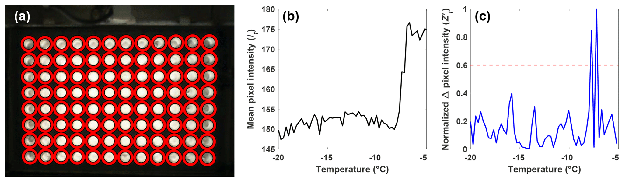
Figure 2(a) Automatic detection of the wells (red circles) using a CHT. (b) Light intensity, or It, of a single well as a function of temperature as observed by the webcam, and (c) the normalized change in pixel intensity, , for the same well as in (b) between subsequent pictures taken during an experiment, as a function of temperature. The most intense peak corresponds to the ice nucleation temperature, and the second-most intense peak is due to the slow freezing of the solution after nucleation. The red dashed line represents the 0.6 threshold required for a well to be classified as frozen.
2.1.2 Freezing detection
With the well locations identified, the intensity values of the pixels within each well are averaged for each image recorded during an experiment (It). The change in It between subsequent images is used to identify the image where freezing occurred and the corresponding temperature (Fig. 2b). However, due to the slow freezing process, which is limited by the latent heat release, the light transmission of a well continuously changes until the water is completely frozen, as can be seen as two large peaks in Fig. 2c. To correctly identify the point in time when ice nucleation and not just freezing within the well occurs, the maximum change in It between subsequent images is normalized to 1 using the following procedure:
First, the Z score (Zt) of It is taken to level out differences in illumination within the 96-well tray:
where μ and σ are the mean and standard deviation of It for all images of a well, respectively. The absolute value of the time derivative or the change in Zt between subsequent images (dt) is given as
is then normalized to 1 by dividing by the maximum of the well. The normalization ensures that a fixed threshold for the identification of ice nucleation can be used rather than relying on a fixed change in light transmission through the well, as done by other drop-freezing setups (Beall et al., 2017). This ensures that the initial freezing detection is independent of the absolute change in light transmission through a well. Based on validation experiments, a threshold value of was found to be best for detecting the initial freezing and to avoid assigning subsequent changes in transparency as a nucleation event due to slow freezing.
2.2 Bath leveler
Due to the thermal contraction of the ethanol in the chilled bath between 0 and −30 ∘C, the ethanol level within the bath decreases during an experiment, affecting the immersion level of the wells and thus the thermal contact. It has been shown that large vertical gradients of up to 1.8 ∘C can exist between the bottom of a well and the air above it in block-based drop-freezing setups (Beall et al., 2017). We anticipate vertical gradients to be reduced in DRINCZ due to the direct contact between the cooling medium (ethanol) and the well tray. Therefore, we incorporated a bath leveler composed of a level sensor and solenoid valve to ensure that the ethanol level remains constant. The level sensor (Honeywell LLE 102101 liquid level sensor) detects when the ethanol falls below a fixed level relative to the wells and triggers the opening of the solenoid valve (Kuhnke 64.025, 12 VDC valve), allowing additional ethanol to flow into the bath. The level sensor and solenoid are monitored and controlled using a “sketch” written in Arduino (Arduino Uno Rev3 SMD). In order to minimize thermal gradients by adding warm ethanol to the bath, the ethanol is precooled to 0 ∘C using an ice water bath and then added through a copper pipe that extends to the bottom of the bath. Thus, the bath leveler ensures that the wells remain in good thermal contact due to a constant level of ethanol during experiments, while minimizing temperature fluctuations within the bath. The resulting increased reproducibility of experiments due to the bath leveler is discussed in Sect. 3.4.
The validation of the instrument is presented in four sections, with the first discussing the temperature calibration, followed by a discussion on the observed bias in freezing, the quantification of instrumental uncertainty and, lastly, the improved reproducibility of DRINCZ due to the addition of the bath leveler.
3.1 Temperature calibration
The temperature reported as the freezing temperature is based on the ethanol bath temperature measured by the LAUDA chiller (Tlauda). In order to correct for the difference between the temperatures of the sample in the wells (Twell) and Tlauda, a temperature calibration was performed. The calibration was conducted by measuring the temperature (type-K thermocouple) within the four corner wells and a center well of the 96-well tray (Fig. 3a). The same thermocouple was used for all the well temperature measurements to avoid biases between different thermocouples. The wells were filled with 50 µL of ethanol instead of water to extend the calibration across the entire experimental temperature range of DRINCZ without the interference of freezing. The temperature bias between the wells and Tlauda was measured every 1 ∘C while the bath was cooled at the typical ramp rate of 1 ∘C min−1. The calibration was performed three times for each well (Fig. 3b). Not surprisingly, we found that the ethanol temperature in the bath was consistently lower than the temperature in the five calibration wells, and the difference between bath and well temperature increased linearly as the bath temperature decreased. Based on these results the linear function , with Tlauda in ∘C (black line in Fig. 3b), was derived to correct the well temperature. The maximum standard deviation taken as the temperature difference between the temperature fit, and the individual well temperature was ±0.6 ∘C.

Figure 3(a) Locations of the type-K thermocouples tested during the temperature calibration. Additionally, the temperature difference between the LAUDA temperature and the ethanol bath was measured at the indicated location (black open circle). (b) The temperature bias between the wells and ethanol bath is displayed versus the LAUDA bath temperature. The linear temperature correction is shown in black.
3.2 Freezing bias across the 96-well tray
The temperature calibration discussed above revealed potential variations in the well temperatures between the corner and the center wells. We thus quantified the bias for individual wells but conclude that it is within the instrument experimental error as discussed below. To do so, 20 pure-water (Molecular Biology Reagent, W4502, Sigma-Aldrich; hereafter referred to as SA water) experiments were analyzed. SA water was chosen for this analysis due to its homogeneity and low freezing temperature, where the observed spread in well temperature was maximized (see Fig. 3). For each well the median freezing temperature (or temperature when FF =0.5; ) was compared to the median freezing temperature of the four corner wells () used for the temperature calibration (see Figs. 3a and A2 for the distribution in freezing temperatures of the wells). The difference between and () is shown in Fig. 4a. The red (blue) shading indicates a warm (cold) bias and signifies that the solution in these wells is exposed to warmer (colder) temperatures than the average of the four reference wells. The higher concentration of red shades in the middle of the tray suggests that the center of the tray is exposed to as much as 1.5 ∘C warmer ethanol flow than the tray periphery. Indeed, the chilled ethanol circulates clockwise in the LAUDA chiller, and thus the freezing appears to track the flow (arrows in Fig. 4). Thus, the ethanol circulation explains the observed bias in freezing temperatures across the well plate. The same analysis procedure was applied to the same 20 samples separated by user (12 and 8 experiments), and a similar bias was observed (see Fig. A3). Therefore, the reported bias is instrumental and reproducible, and any potential user bias can be excluded. The bias was found to be statistically significant at the 95 % confidence interval for 30 % of the wells and resulted in an overall bias of 0.23 ∘C (see Fig. 4b and Appendix A). As such, a well-by-well bias correction was developed and tested as described in Appendix A. Although the bias correction performed as expected, the bias of 0.23 ∘C falls within the instrumental uncertainty as discussed in Sect. 3.3 and is therefore not applied to DRINCZ measurements by default. Nevertheless, the potential benefits and impacts of a bias correction are discussed in the following section.
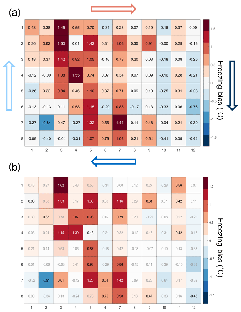
Figure 4(a) Bias in the freezing of SA water ( in ∘C) based on the median value of each well over 20 experiments relative to the median temperature of freezing for the four corner wells used during the temperature calibration. A positive (negative) bias indicates that the wells experience a warmer (colder) temperature than the four corner wells used for temperature calibration and therefore freeze at lower (higher) temperatures than reported. The arrows represent the ethanol circulation in the chiller, and the color represents the temperature trend of the ethanol as it circulates in the bath with, dark blue being the coldest and red the warmest. (b) Mean freezing bias of SA water between the four reference wells and each well (). Positive (negative) values indicate, as denoted by shades of red (blue), wells that systematically freeze at colder (warmer) temperatures and therefore experience warmer (colder) temperatures than reported. Statistically insignificant biases as determined by Welch's t test (see Eq. A1) are depicted with white shading.
Impact of bias correction on frozen fraction
By accounting for the bias in freezing temperature across the 96-well tray by first applying the temperature calibration and then the bias correction such that corrected well value ( becomes
the slope of the FF curves steepens and becomes smoother, which is expected as the observed freezing temperatures become more constrained (see Fig. 5). Although the median freezing temperature with and without the bias correction only changes by 0.2 ∘C (consistent with the correction of the mean bias of 0.23 ∘C found above), the narrowing of the freezing temperature distribution is significant at the 95 % significance level (Welch's t test, see Eq. A1). This result shows that by using the spatially dependent freezing information of a well from optically based drop-freezing instruments like DRINCZ, temperature can be better constrained. Such a bias correction should also be applicable to freezing methods that use block-based cooling, where gradients across the block have been observed or modeled (Beall et al., 2017; Harrison et al., 2018).
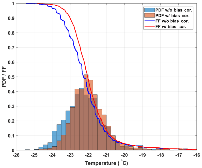
Figure 5Histograms representing the probability distribution functions for freezing temperatures of the 20 SA water experiments without (blue bars) and with (red bars) the bias correction. The calculated cumulative distribution functions, or frozen fraction curves without and with the bias correction, are represented as the blue and red lines, respectively.
3.3 Instrument uncertainty
The instrumental uncertainty for DRINCZ is assessed by using the standard deviation in the observed freezing temperatures of the SA water experiments across all wells in combination with the error in the temperature of the wells established during the temperature calibration. The standard deviation of the freezing temperature of the SA water is dependent on FF, with a minimum at 0.5 FF (Fig. 6a). This dependence is expected, as the 0.5 FF corresponds to the most likely temperature for the SA water to freeze and, therefore, should show the least variability across the 20 experiments used in the analysis. Furthermore, by using the 0.5 FF, the influence of contamination and outliers is minimized. The standard deviation at each FF is the uncertainty due to the instrument as well as the variability in the freezing temperature of the SA water and represents the upper limit of the instrumental uncertainty. Given the contribution to the uncertainty due to the variability in the freezing temperature of the SA water, the standard deviation at FF=0.5 can be used as the upper limit of the instrumental uncertainty across the entire FF range. Incorporating a bias correction results in a negligible average difference in the standard deviation (as shown by dashed lines in Fig. 6a). Thus, the upper limit of the instrumental precision is ±0.3 ∘C (the mean of the standard deviation of freezing temperature over the entire freezing spectrum).
Although the instrumental precision indicates that DRINCZ is very reproducible (±0.3 ∘C), the accuracy in the reported temperature must be accounted for. Based on the temperature calibration, the standard deviation of the well temperatures is temperature dependent. At the coldest temperatures of the freezing range of the SA water ( ∘C), the standard deviation of the well temperatures is largest, likely due to the increased gradient between the bath and air temperature, and therefore the importance of the ethanol circulation through the bath is increased. To account for this temperature dependence, the maximum standard deviation of ±0.6 ∘C from the temperature calibration, corresponding to the lowest observable freezing temperature in DRINCZ (freezing temperature of SA water), is used. Therefore, when accounting for both the precision of the measurements and the accuracy of the temperature, the overall uncertainty of the reported freezing temperature of a well in DRINCZ is ±0.9 ∘C. This value is comparable to other recently developed drop-freezing techniques, which report uncertainties ranging between ±0.9 ∘C (Harrison et al., 2018) and ±2.2 ∘C (Beall et al., 2017).
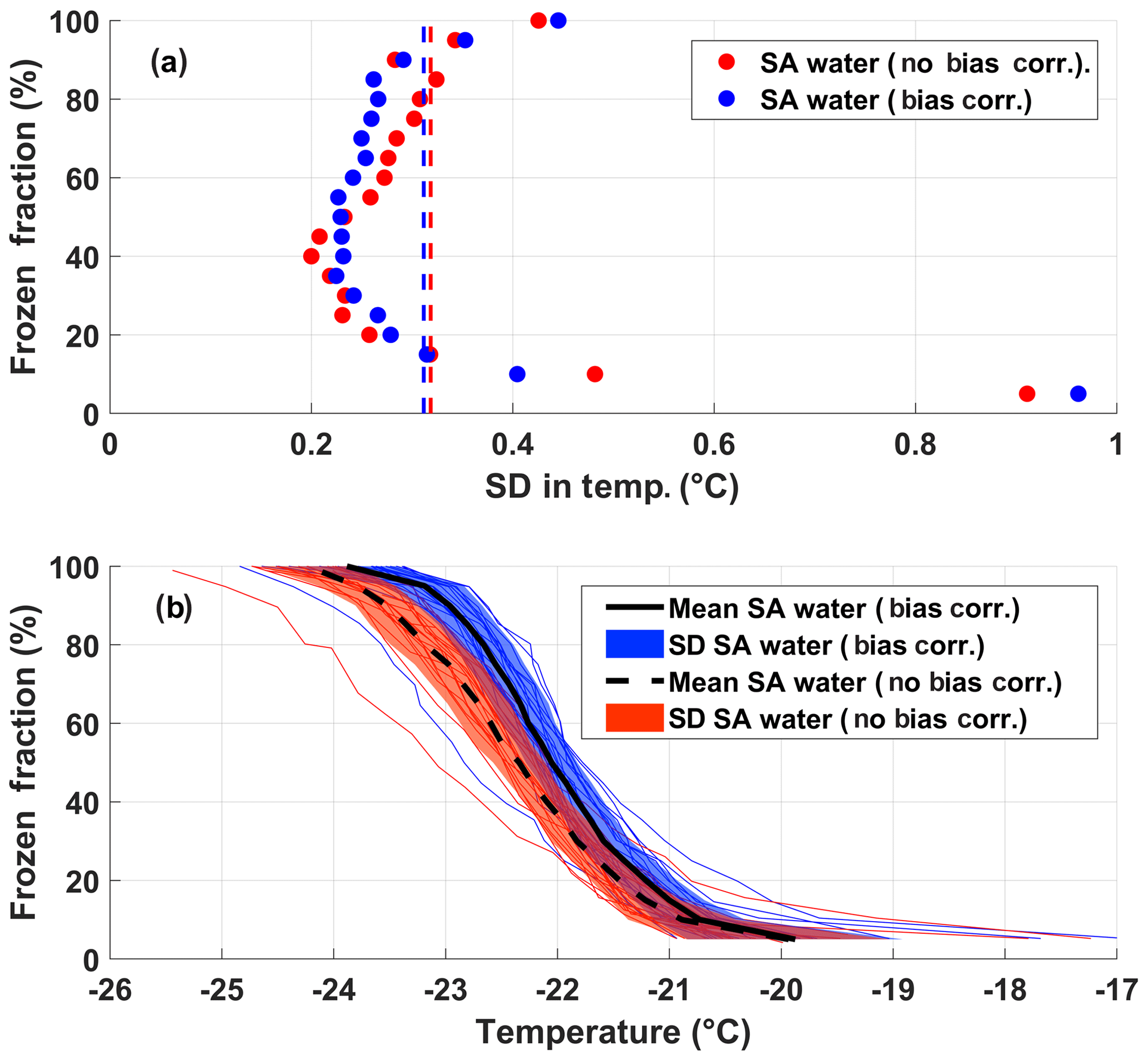
Figure 6(a) FF and the corresponding standard deviation (SD) of the freezing temperatures from the 20 SA experiments with and without the bias correction, shown as blue and red dots, respectively. The red and blue dashed lines represent the standard deviations in temperature averaged over all FF values without and with the bias correction, respectively. (b) The FF of the 20 SA water experiments as a function of temperature with and without the bias correction (thin blue and red lines, respectively). The colored shading represents the standard deviations of the SA water from the mean freezing temperature with (solid black line) and without (black dashed line) the bias correction.
3.4 Importance of the bath leveler
To assess the impact of the decreasing ethanol level on experiments in DRINCZ, 32 experiments with SA water without a bath leveler were compared to the 20 SA water with a bath level sensor, the same 20 SA water discussed in the previous section. Figure 7a shows that the bath sensor reduces the spread in freezing temperatures observed. The decrease in the 0.5 FF temperature without the bath leveler is due to a larger gradient between the aliquot and the bath temperatures; thus the well is warmer than expected, requiring further cooling to observe freezing. The additional cooling in combination with the variable starting level of the ethanol relative to the wells in the cases of no bath leveler is responsible for the longer freezing tail of the FF curve (blue line) at higher FFs. Without the bath leveler, the initial height of ethanol relative to the wells is user dependent and not reproducible, leading to both the higher and lower observed freezing temperatures.
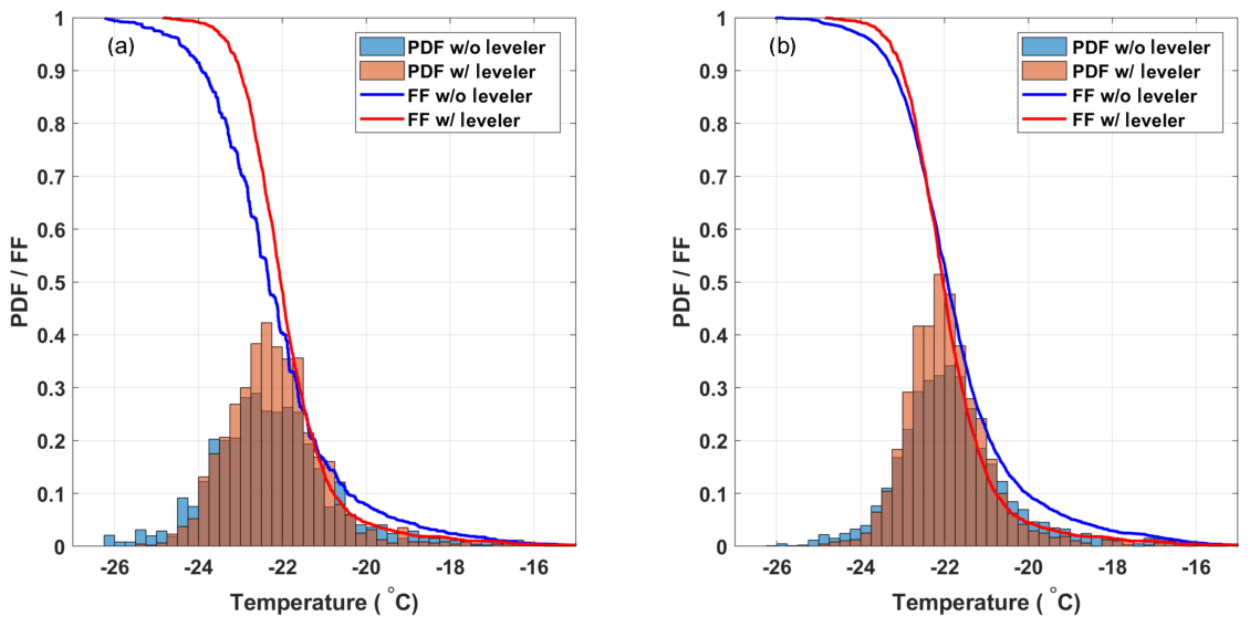
Figure 7(a) Comparison of the freezing temperature of SA water without (32 experiments; blue) and with (20 experiments; red) the bath leveler. The histograms are normalized to represent the PDF of the freezing temperatures, and the lines represent the mean FF curves of the SA water experiments. (b) Shows the same as panel (a) except that a bias correction is applied to both sets of experiments.
Although the median freezing temperature (FF=0.5) only decreased by 0.25 ∘C without the bath leveler, the freezing curves steepen when the bath leveler is incorporated into DRINCZ, leading to a decrease in the standard deviation from ±1.4 to ±1.0 ∘C over the entire FF range. A bias correction applied following the procedure in Sect. 3.2 reduces the issues associated with a variable bath level as seen by the similar FF curves and histograms normalized using the probability density function (PDF) estimate in Fig. 7b for experiments with and without the bath leveler. The difference in mean freezing temperatures decreases to 0.05 ∘C at FF=0.5, and the standard deviation of the SA water freezing temperature without the leveler decreases from ±1.4 to ±1.2 ∘C over the entire FF range. This decrease is expected, as the bias correction is designed to reduce the spread in freezing temperatures within the 96 aliquots. Although the bias correction reduces the need for a bath leveler in DRINCZ, the bias is instrument dependent and may be less pronounced in other drop-freezing setups. Therefore, we recommend the use of a bath leveler in any bath-based drop-freezing device.
To verify the performance of DRINCZ in the context of other published drop-freezing techniques, we use the SA water experiments to characterize the instrumental background (Sect. 4.1) and perform freezing experiments with NX-illite suspensions (Sect. 4.2). To demonstrate applicability of the instrument to analysis of field samples, the evolution of the ice-nucleating ability of atmospheric aerosol particles collected in snow samples at the Sonnblick Observatory in the Hohe Tauern region of Austria during a midlatitude storm system is assessed in Sect. 4.3. Lastly, some uncertainties associated with measuring INPs in snow samples (Sect. 4.4) and further validation of DRINCZ through dilutions are discussed (Sect. 4.5).
4.1 Background of DRINCZ
The background freezing due to the experimental technique and the SA water used to suspend and dilute samples must be known to discriminate freezing events due to the sample from freezing events due to the water used. Furthermore, an SA water sample is run as a standard at the beginning of each measurement day to ensure that the system is operating correctly. The 20 SA water experiments are therefore used to assess the instrument background freezing. It is important to note that in cases where solvents other than SA water are used or where contamination from a sampling technique (e.g., snow collection or impinger measurements) is possible, a different background calculation must be used to accurately assess the freezing ability of a sample. The background of DRINCZ, when used with SA water, is calculated by fitting the 20 SA water experiments with a five-parameter Boltzmann fit. The five-parameter version was chosen to account for asymmetry (Spiess et al., 2008) in the freezing of the SA water, but due to the minimum and maximum values of FF, given as 0 and 1, respectively, the fit reduces to three parameters and takes the form
where FFBGfit is the fitted FF of the SA water as a function of the observed freezing temperatures of the SA water, TfrzBG, and the fitting parameters, a, b and c, represent the slope of the fit (a=1.9651), the inflection point () and the asymmetry factor (c=0.6160), respectively. The value of 1 in the numerator represents the maximum FF. The fit and associated coefficients (including 95 % confidence range and r2) are shown in Table 1 and Fig. 8, respectively.
Table 1Coefficients for the three-parameter Boltzmann fit of the SA water freezing background and values bound by the 95th-percentile confidence interval.
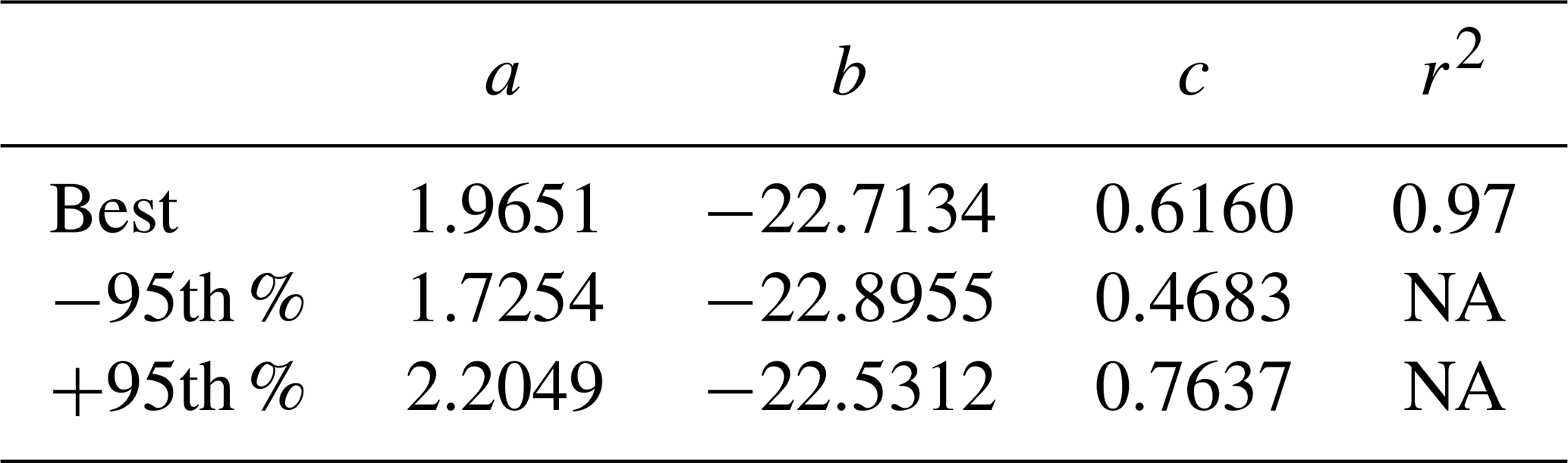
NA: not available.
The fitted freezing background is used to correct for the contribution of SA water to the observed freezing of a sample. To account for the presence of multiple ice-nucleating particles coexisting in a single well, the background is removed by subtracting the differential nucleus concentration of the background from that of the sample (Vali, 1971, 2019). The differential nucleus concentration (k(T)) is initially defined in Vali (1971) as
where N(T) is the number of unfrozen aliquots at the beginning of a temperature step, while ΔN is the number of aliquots that freeze during the temperature step (between pictures), or ΔT.
The background-corrected differential nucleus concentration (kcorr(T)) is obtained by
where ksam(T) and kbg(T) are the sample and background differential nucleus concentration, respectively. The background-corrected FFcor(T) is then achieved by inverting Eq. (9) and taking the cumulative sum of kcorr(T):
An example of the impact of the background correction on the FF of the diluted snow sample collected on 30 November 2017 (discussed in Sect. 4.3) is shown in Fig. 8.
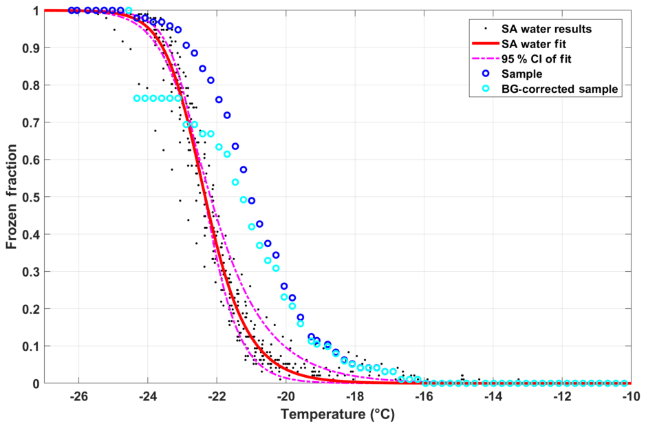
Figure 8SA water data (black dots) and corresponding fit (red line; Eq. 8), including the 95th-percentile confidence interval (CI; dashed–dotted magenta lines). The blue circles represents the diluted snow sample collected on 30 November 2017, which is then corrected for the contributions of freezing from the SA water using the background correction (FFcor(T) as described in Eq. 11; cyan circles).
4.2 Comparison of DRINCZ to other immersion freezing techniques
To validate the performance of DRINCZ, we use different weight percent suspensions of NX-illite to compare the results from DRINCZ to those summarized in Hiranuma et al. (2015), Beall et al. (2017) and Harrison et al. (2018). In the atmosphere, illite constitutes up to ∼40 % of the transported dust fraction (Broadley et al., 2012; Murray et al., 2012), making it an excellent surrogate for atmospherically relevant dust. An initial stock suspension of 0.1 wt % NX-illite was prepared with SA water and then diluted to produce mass concentrations of NX-illite of 0.05 and 0.01 wt %. The suspensions were manually shaken for 30 s, poured into a dispensing tray and then immediately pipetted into the well plate. Triplicates of each suspension concentration were investigated with DRINCZ (see Fig. A4 for FF curves) and then normalized to the number of active sites per BET-derived surface area (nsBET) using a variation of Eq. (2) as follows:
where SABET is the BET surface area of the particles used (NX-illite) and CNX is the mass concentration of NX-illite in an experiment.
The nsBET of NX-illite calculated using Eq. (12) from the measurements made with DRINCZ and background corrected (using Eq. 11) falls within the results from Hiranuma et al. (2015), Beall et al. (2017) and Harrison et al. (2018) (Fig. 9). In theory, nsBET should be insensitive to concentration as the number of ice-nucleating sites is normalized to the total surface area. Indeed, the samples differing in weight percent overlap to an extent (Fig. 9). Furthermore, the lower weight percent suspensions extend the observable nsBET to higher values and colder temperatures. Similar to the observations of Harrison et al. (2018), the data points from the 0.01 wt % suspension appear as outliers at the warmest temperatures. However, it is not possible to determine if these outliers are due to random freezing events that occur at high temperatures and therefore produce elevated cumulative nsBET values at lower temperatures or if they are due to an uneven distribution of the active sites in each aliquot that may result from diluting a single stock suspension rather than preparing individual weight percent suspensions (Harrison et al., 2018). Thus a spread equivalent to or less than the spread in the concentrations, up to an order of magnitude in this case, can be expected. Furthermore, considering the ±0.9 ∘C uncertainty, depicted by the horizontal error bars, the differences between concentrations are not significant. They fall within the same range as the measurements of Beall et al. (2017) and between BINARY and Leeds-NIPI and IR-NIPI at colder temperatures (Fig. 9). The overlap between the nsBET measured with DRINCZ and the NX-illite parameterization (Hiranuma et al., 2015) indicate that DRINCZ is capable of accurately measuring the concentration of INPs and their active sites in the immersion freezing mode (Fig. 9).
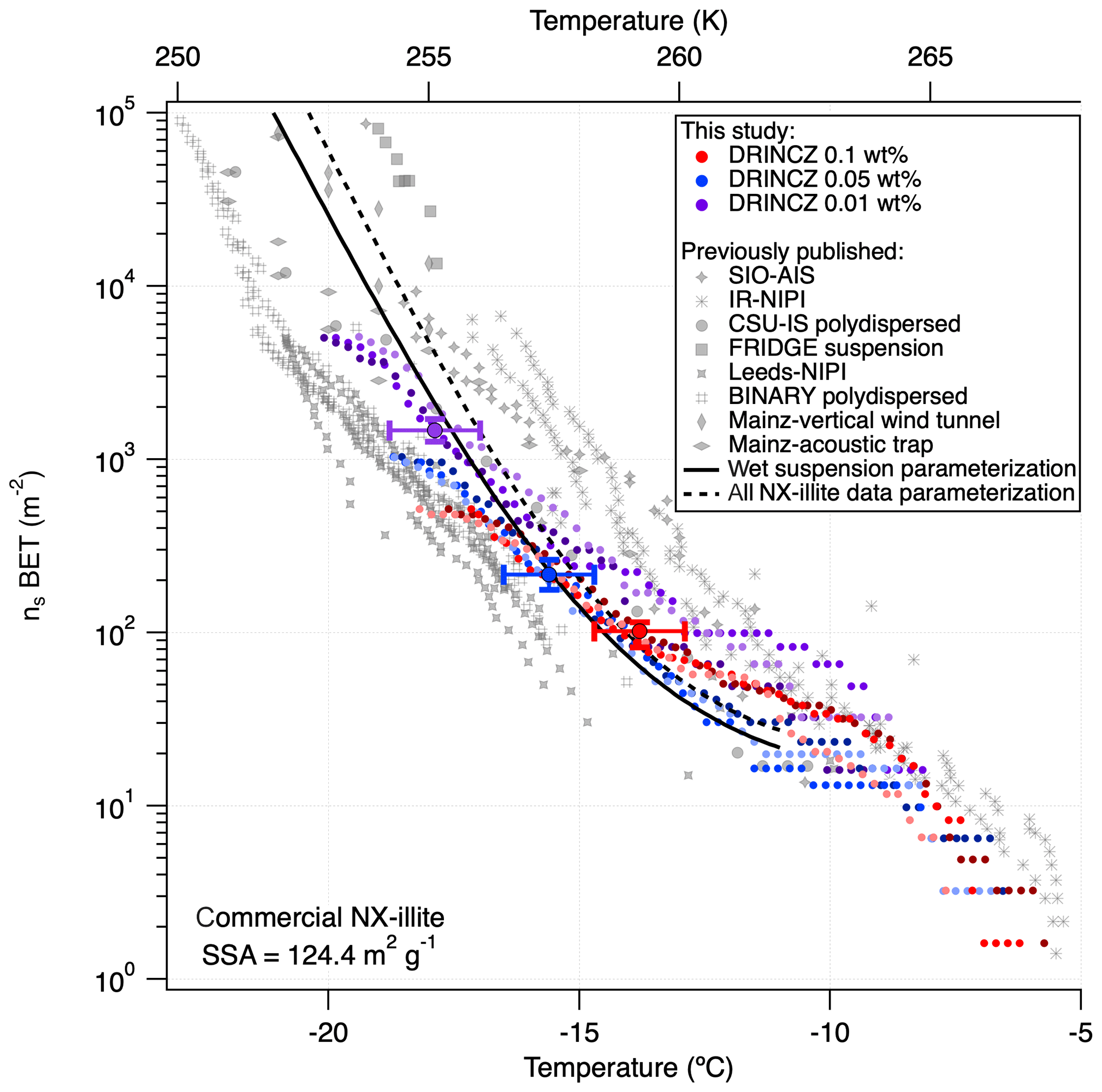
Figure 9Triplicates of nsBET (depicted by shading of the same color) as a function of temperature for three concentrations of NX-illite, 10−3 g mL−1 (red dots), g mL−1 (blue dots) and 10−4 g mL−1 (purple dots), measured by DRINCZ. An example of the temperature uncertainty and the uncertainty due to the background correction are depicted for each weight percent as horizontal and vertical error bars, respectively. Literature values from Hiranuma et al. (2015), Beall et al. (2017) and Harrison et al. (2018) are shown for comparison. nsBET was calculated using a BET surface area of 124.4 m2 g−1 (Hiranuma et al., 2015).
4.3 Ice-nucleating particle concentrations in snow samples from a mountaintop observatory in Austria
In order to demonstrate the performance of DRINCZ, snow samples collected between 27 and 30 November 2017 at the Sonnblick Observatory (SBO) were analyzed. The SBO is located at 3106 m on the summit of Mt. Sonnblick in the Hohe Tauern Region of Austria and has previously been used for cloud microphysical measurements (e.g., Beck et al., 2018; Puxbaum and Tscherwenka, 1998). Freshly fallen snow was collected from a wind-sheltered area where the snow could not drift. A stainless-steel shovel (Roth) was conditioned with snow by turning (10 times) in the surface snow next to the sampling site prior to sampling. The snow was then sampled into sterile Nasco Whirl-Paks (Roth) and then melted at room temperature (20 ∘C), immediately after which aliquots of snow meltwater were filled into sterile centrifugation tubes (15 mL; Falcon tubes) and stored at −20 ∘C. The samples were shipped and stored frozen until processed with DRINCZ at the Atmospheric Physics Laboratory at ETH Zürich to minimize any bacterial growth or changes due to liquid storage (Stopelli et al., 2014). The snowfall collected at SBO occurred during two snowfall events. The first event began on 25 November and ended overnight on 26 November (early hours of 27 November), while the second event (28–30 November) was associated with an intensifying upper-level trough, a developing surface cyclone, a strong cold front and an associated secondary low (see Figs. A5 and A6).
The frozen fractions of five different snow samples were determined using DRINCZ, and the cumulative concentration of active sites (or INP(T), see Eq. 1) was normalized per liter of meltwater (nmw; Fig. 10). Overall, the nmw values of the snow samples fall within the range of previously reported values for precipitation samples (Petters and Wright, 2015) except for the 30 November sample. Within these samples, we identify (1) a particularly active snow sample (28 November), (2) samples having intermediate ice nucleation activity (27 and 29 November) and (3) a least-active sample (30 November). We attempt to compare these snow samples based on their air mass origin.
The snowfall sampled on 28 November had the highest nmw of all collected samples (Fig. 10). The meteorological conditions and a comparison of back trajectories indicate that the air mass was associated with the warm sector of a synoptic system (Fig. A7) that originated from North America and the North Atlantic that then crossed France and Switzerland before arriving at SBO (Fig. A8). In contrast, the arctic air mass responsible for the snowfall sampled on 27 November originated over Svalbard before crossing Iceland, the British Isles, northern France and Germany (Fig. A8).
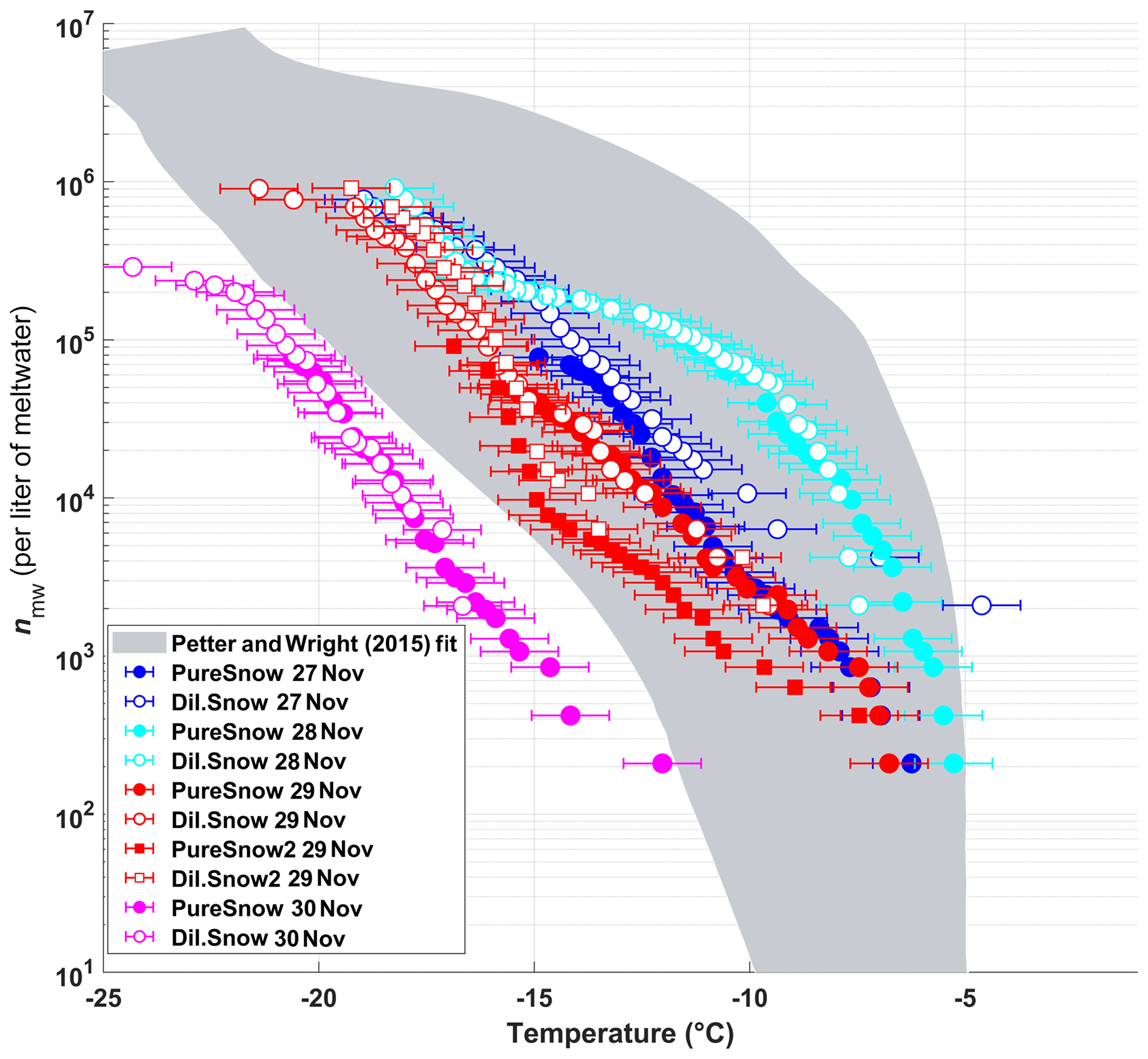
Figure 10The cumulative number of active sites per liter of meltwater (nmw) of snow for undiluted snow (filled) and of snow samples diluted by a factor of 10 (white-filled symbols) as a function of temperature. The colors represent the different sampling days. On 29 November two samples were taken, and the second sample of the day is indicated by square symbols. The shaded area represents the previously reported nmw from precipitation events as described in Petters and Wright (2015). The error bars represent the instrumental temperature uncertainty of ±0.9 ∘C.
Even though the local conditions at SBO did not change significantly between 28 and 29 November, a decrease in nmw was observed relative to 28 November, and nmw gradually decreased between the first and second sample on 29 November (Fig. 10). The back trajectories show that the origin of the air mass changed from North America and the North Atlantic on 28 November to exclusively originating over the North Atlantic on 29 November (Fig. A8). Additionally some of the back trajectories on 29 November show an increased interaction with the boundary layer over Europe (Fig. A8). Nevertheless, the decrease in nmw suggests that if boundary layer aerosols from parts of Europe did reach the precipitating clouds at the SBO, they are less efficient INPs than the marine aerosols (Lacher et al., 2017, 2018) associated with the samples on 27 and 28 November.
Finally, the lowest nmw values observed were from meltwater collected on 30 November. The cold frontal passage and associated cold-air advection caused the temperature to drop by 6 ∘C by noon on 30 November (Fig. A7), and the nmw in the associated snowfall decreased substantially, exceeding the lower limit of previously reported nmw values (Petters and Wright, 2015, Fig. 10). The decrease in nmw, however, cannot be explained solely by the origin of the air mass, as the arctic air mass on 27 November also crossed similar parts of the UK or had significant interaction with the marine boundary layer. Nevertheless, the concentration of INPs in the sea surface microlayer is variable, and the efficiency of emitting marine INP from the surface is wind speed dependent (DeMott et al., 2016; Irish et al., 2017; McCluskey et al., 2018; Wilson et al., 2015). Therefore, even though the trajectories on 27 and 30 November interacted with the marine boundary layer, they may contain different concentrations of INPs, yielding the observed differences in nmw. In addition to air mass origin, it has been shown that precipitation efficiently removes INP and thus influences nmw (Stopelli et al., 2015). Indeed, the most upstream precipitation (see Fig. A8) corresponds to the sample collected on 30 November, which has the lowest nmw. Therefore, the most efficient INPs could have been removed in the upstream precipitation, contributing to the observed decrease in nmw.
The differences in nmw could not be rectified by a single metric in this study, but rather a combination of factors likely led to the observed variability. In particular, as the warm sector of the cyclone approached the sampling site (28 November), nmw increased. Conversely, after cold frontal passage (30 November) the nmw decreased. Back trajectories indicate that the air mass source region and the amount of upstream precipitation differed between the two sectors of the cyclone. This result is consistent with previous studies that suggest that air mass origin (e.g., Ault et al., 2011; Creamean et al., 2013; Field et al., 2006; Lacher et al., 2017, 2018) and upstream precipitation (Stopelli et al., 2015) influence the INP concentration. Furthermore, the dependence on the long-range air mass history to the observed variability in nmw suggests that local sources are not responsible for the observed INPs.
4.4 Limitations of snow meltwater sample comparisons
One limitation when comparing snow samples collected at different times and locations is the unknown number of aerosols, INPs and ice crystals that contributed to the collected meltwater. Since nmw depends on the number and mass of the ice crystals within a snow sample, the meltwater volume or density of each snowflake influences nmw. For example, snow-to-liquid ratios, which can be used as a proxy for snow flake density and meltwater equivalent, can vary between a 5-to-1 ratio in heavy wet snow and a 100-to-1 ratio in powdery snow (Roebber et al., 2003). However, even when considering this variability in the required amount of snow to produce the same volume of ice crystal meltwater, nmw would only differ by a factor of 20. As can be seen in Fig. 10, nmw varies by 2 orders of magnitude or more between 28 and 30 November, and the difference is therefore robust. Additionally, heavy wet snow has been found to occur in the warm core of a synoptic system, while lighter, more powdery snow was found in the air mass after cold frontal passage, where air temperatures are colder (Roebber et al., 2003). As the nmw on 28 November was collected in the warm sector and the sample on 30 November was after the cold front, differences in snow density may lead to an underestimation in the difference between the nmw values of these two samples. Therefore, we recommend that future studies also consider the snow water equivalent when comparing the nmw, as this could influence the nmw by a factor of 20 or more.
Another uncertainty with using precipitation samples for analyzing INP concentrations is associated with aerosol scavenging and chemical aging (e.g., Petters and Wright, 2015). As previously mentioned, the samples were stored frozen to avoid any decrease in ice-nucleating ability associated with storage (Stopelli et al., 2014), and therefore degradation is likely not an issue in this study (Wex et al., 2019). The ability of a falling ice crystal to scavenge aerosols or rime cloud droplets depends on the ice crystal habit and size and the difference between the fall velocity of the crystal and the interstitial aerosol or cloud droplets. With the exception of interstitial aerosol concentration, which has been shown to influence nmw by a factor of 2 (Petters and Wright, 2015), these factors are all important when estimating snow density and thus make it difficult to disentangle their effects on nmw. Therefore, there is value in future studies of INPs in MPCs in investigating the INP concentrations in cloud water, interstitial aerosols and snow samples.
4.5 Ice-nucleating particle concentrations in diluted snow samples
In order to extend the reported temperature range of DRINCZ, the snow samples were also diluted by a factor of 10 with SA water (see Eq. 2). The dilutions (open symbols) overlay the pure samples except at the warmest temperatures, where, as previously mentioned, a single freezing event can lead to an increase in nmw of an order of magnitude relative to the undiluted sample. This effect is especially evident on 27 November, when the first few wells of the diluted sample (open blue circles) froze at the same or higher temperatures than the undiluted sample (filled blue circles) and led to an increase in nmw of up to an order of magnitude. However, this issue has been previously observed when diluting from stock suspensions (Harrison et al., 2018), which is similar to diluting a snow water sample. Therefore, the dilutions further validate DRINCZ as an INP measurement technique.
We describe and characterize DRINCZ as a newly developed drop-freezing instrument for quantifying the ability of aerosols to act as ice-nucleating particles in the immersion freezing mode. The instrument uncertainty is ±0.9 ∘C, similar to previously published drop-freezing techniques. We show that thermal contraction of ethanol as a coolant used in bath-based drop-freezing techniques increases temperature variations within the sample. This issue can be corrected by incorporating a bath leveler, which ensures that the coolant level in the bath remains constant during an experiment. Typical drop-freezing methods report temperature measured in the corner wells of a 96-well tray, at the edge of a cooling block or within the block itself (Beall et al., 2017; Hill et al., 2014; Stopelli et al., 2014). Here we show that by making use of the freezing sequence of pure water aliquots, the spatial pattern of temperature bias in the 96-well tray can be assessed. Although variations are within the instrumental uncertainty of DRINCZ and are not used for DRINCZ data analysis, we present our detailed analysis of this potential bias and draw attention to this issue for other drop-freezing techniques. The calculated bias correction increases the precision of drop-freezing setups and is an alternative to computationally expensive heat transfer simulations (Beall et al., 2017). Validation experiments conducted with NX-illite showed good agreement with data reported in the literature for this INP standard.
We exemplify the use of DRINCZ by measuring the concentration of INP in snow samples collected at the Sonnblick Observatory in Austria. The observed INP concentrations are within previously reported values as summarized in Petters and Wright (2015) for the same temperature range as investigated here (−22 to 0 ∘C). Differences in INP concentration can be explained by differing sectors of a midlatitude cyclone. As the warm sector of the cyclone approached the sampling site, the INP concentration increased, while after the cold front passed, the INP concentration decreased. Back trajectories indicate that the air mass source region and the amount of upstream precipitation differed between the two sectors of the cyclone. This result is consistent with previous studies that suggest that air mass origin (e.g., Ault et al., 2011; Creamean et al., 2013; Field et al., 2006; Lacher et al., 2017) and upstream precipitation (Stopelli et al., 2015) influence the INP concentration. This suggests that INPs in precipitation samples are likely transported from specific source regions rather than originating from local sources. Thus identifying the specific sources responsible for INP and their transport pathways is essential for accurately modeling the ice phase in clouds and, ultimately, climate.
The code for detecting the wells and determining when a freezing event occurs is written in MATLAB® and available upon request from the authors.
The data presented in this publication are available at the following DOI: https://doi.org/10.3929/ethz-b-000369839 (David et al., 2019).
A1 Freezing bias by user
The 20 SA water experiments were performed over a 3-month period by two users. The SA water was unaffected by aging over this period, as it originated from varying bottles distributed by the manufacturer (Sigma-Aldrich). The user bias was calculated the same way as the bias for all 20 experiments. The bias is relative to the median freezing temperature of the four corner wells obtained by the respective user. As can be seen in Fig. A3, the pattern of freezing bias is consistent regardless of the user. This similarity indicates that the reported bias is instrumental and not user specific.

Figure A1Schematic of the 96-well tray holder from above (a) and the side (b); dimensions are in millimeters.
A2 Bias significance and correction
To ensure that the observed bias is statistically significant, a two-sample, two-tailed t test was performed. In particular, Welch's t test was used due to the different number of samples between the combination of the four reference wells (20 experiments ×4 wells =80 values) and each well (20 experiments ×1 well =20 values) and the different variance in freezing for each well (Derrick and White, 2016). In Welch's t test the location parameter of two independent data samples is assessed as follows:
where and are the mean freezing temperature of the reference wells and an individual well, respectively. and are the variances in freezing in the reference and the individual wells, and Nw4ref and Nwi are the number of samples for the reference wells and an individual well, respectively. The variance in the freezing temperature of SA water in each well is shown as box plots in the Appendix A (Fig. A2). The temperature of approximately 30 % of the wells was found to be statistically different from the average freezing temperature of the four reference wells at the 95 % confidence level, with a resultant mean bias of 0.23 ∘C (Fig. 4b). Due to a fraction of wells with a statistically significant bias, a correction factor based on the mean bias from the 20 SA water experiments is tested for all wells excluding the four corner wells used as the reference to avoid overfitting the data. Of note, the reported bias is derived based on the freezing range of SA water, from −16 to −26 ∘C. However, based on the relatively constant spread in the temperature calibration data (see Fig. 3b), it is reasonable to assume that the bias has a weak temperature dependence.

Figure A2A side-by-side comparison of box plots for the freezing temperatures of the 20 SA water experiments of the reference wells (left box) and the well represented by the location (right box) of each subplot. The median is shown as a red line, the interquartile range is depicted by the blue box, extreme values not considered outliers (whiskers) and outliers (red crosses) are shown as a function of temperature (in ∘C; y axes).
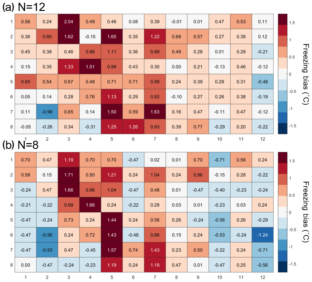
Figure A3(a) Bias in the freezing of SA water (∘C) based on the median value of each well over 12 experiments, and (b) 8 experiments relative to the median temperature of freezing for the four corner wells used during the temperature calibration. A positive (negative) bias indicates that the wells experience a warmer (colder) temperature than the four corner wells used for temperature calibration and therefore freeze at lower (higher) temperatures than reported.
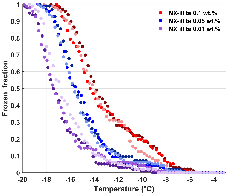
Figure A4Frozen fraction curves of suspensions of 0.1 wt % (red dots), 0.05 wt % (red dots) and 0.01 wt % (purple dots) of NX-illite run in triplicates as shown by shading.
Although the freezing bias was shown to be representative when the SA water data were split into two (8 and 12 samples), it is still necessary to validate its robustness on a larger sample size. In order to artificially increase the sample size of the experiments, the bias was recalculated randomly such that only 90 %, or 18, of the experiments were used. The resultant bias correction was then applied to the remaining 10 %, or 2, of the experiments and tested to see if the mean freezing temperature of the bias-corrected tray was closer to the reference freezing temperature of the four corner wells. This procedure was repeated 1000 times at random. The difference in the median freezing temperature (FF=0.5) and four corner reference wells decreased from 0.23 to 0.04 ∘C, while the standard deviation of the bias-corrected data increased by 0.007 ∘C. Thus, the bias correction performed as expected and reduced the bias in freezing temperature. Nonetheless, this improvement falls within the uncertainty of the instrument, as discussed in Sect. 3.3, and is therefore not applied to DRINCZ measurements by default.
A3 Synoptic summary 27–30 November
The synoptic pattern over Europe on 27 through 30 November produced large variations in both temperature and air mass origin at the SBO. As can be seen from the surface pressure maps shown in Fig. A5, an evolving cyclone tracked across northern Europe before occluding in the vicinity of Denmark. This cyclone produced strong warm advection at SBO on 27 November (see Fig. A7) in advance of the approaching cold front. As the cyclone began to fill over southern Scandinavia, the cold front stalled along the Alps and westerly flow continued at SBO from 28 to 29 November (Fig. A7). Farther west, the cold front reached the Mediterranean, where a secondary low developed along the remnant baroclinic zone (Fig. A6c). This secondary low traversed Italy and rapidly intensified as it crossed the Adriatic Sea before entering the northern Balkans (Fig. A6d). The secondary low and an amplifying ridge over the British Isles forced the cold front over SBO at 00Z on 30 November, when cold-air advection ensued over the SBO region (Fig. A7), as shown by the back trajectories (Fig. A8e and f).
A4 HYSPLIT back trajectories
The HYbrid Single-Particle Lagrangian Integrated Trajectory (HYSPLIT) model (Stein et al., 2015) was run using the interactive web portal (Rolph et al., 2017). The trajectories were calculated using 0.5∘ resolution, and the trajectories were initialized 1000, 2000 and 3000 m above the model terrain height. Although the majority of snow mass growth has been shown to occur between the mountaintop and 1 km above the surface (Lowenthal et al., 2016), these heights were chosen due to the coarse resolution of the model terrain height and the observed sensitivity of the back trajectories to height. HYSPLIT was initialized using the 0.5∘ hourly Global Data Assimilation System (GDAS) archived database, and the vertical velocity was model-based rather than isentropic.
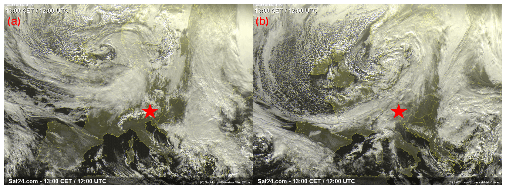
Figure A5Visible satellite image of the storm system impacting the SBO (red star), taken at 12:00 UTC on (a) 27 November and (b) 28 November. Images courtesy of sat24, EUMETSAT, and the Met Office (http://www.sat24.com/history.aspx, last access: 22 March 2019).
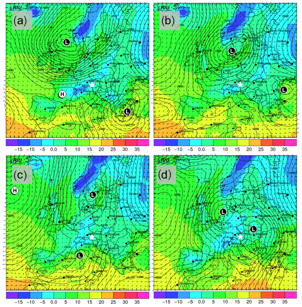
Figure A6Forecasted surface pressure in hectopascals (black contours); 2 m surface temperature (in ∘C; colored shading); and wind vectors (in m s−1; black arrows) for 12:00 UTC on (a) 27, (b) 28, (c) 29 and (d) 30 November. Forecasts are based on model runs initialized on 00:00 UTC of the day of interest (12 h before shown values). Surface low-pressure and high-pressure centers are indicated with L and H, respectively. The location of SBO is indicated with the white star. Images are taken and adapted from the Rhenish Institute for Environmental Research at the University of Cologne (http://www.uni-koeln.de/math-nat-fak/geomet/eurad/index_e.html, last access: 22 March 2019).
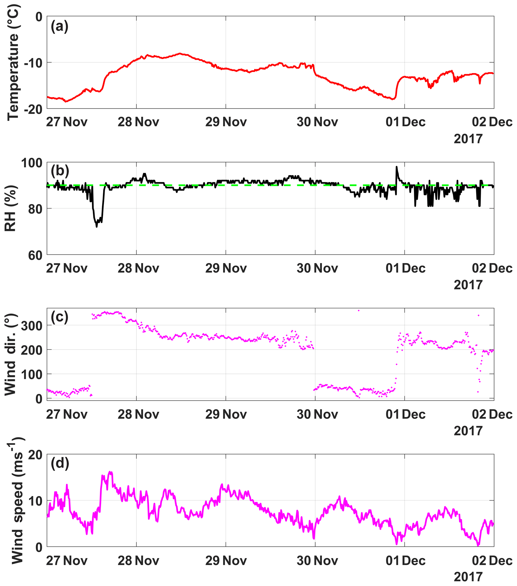
Figure A7(a) Temperature (∘C), (b) humidity (%), (c) wind direction (∘) and (d) wind speed (m s−1) as a function of date, spanning from 27 November to 2 December (in UTC). The humidity when cloud is present at SBO (90 %) is shown (dashed green line).
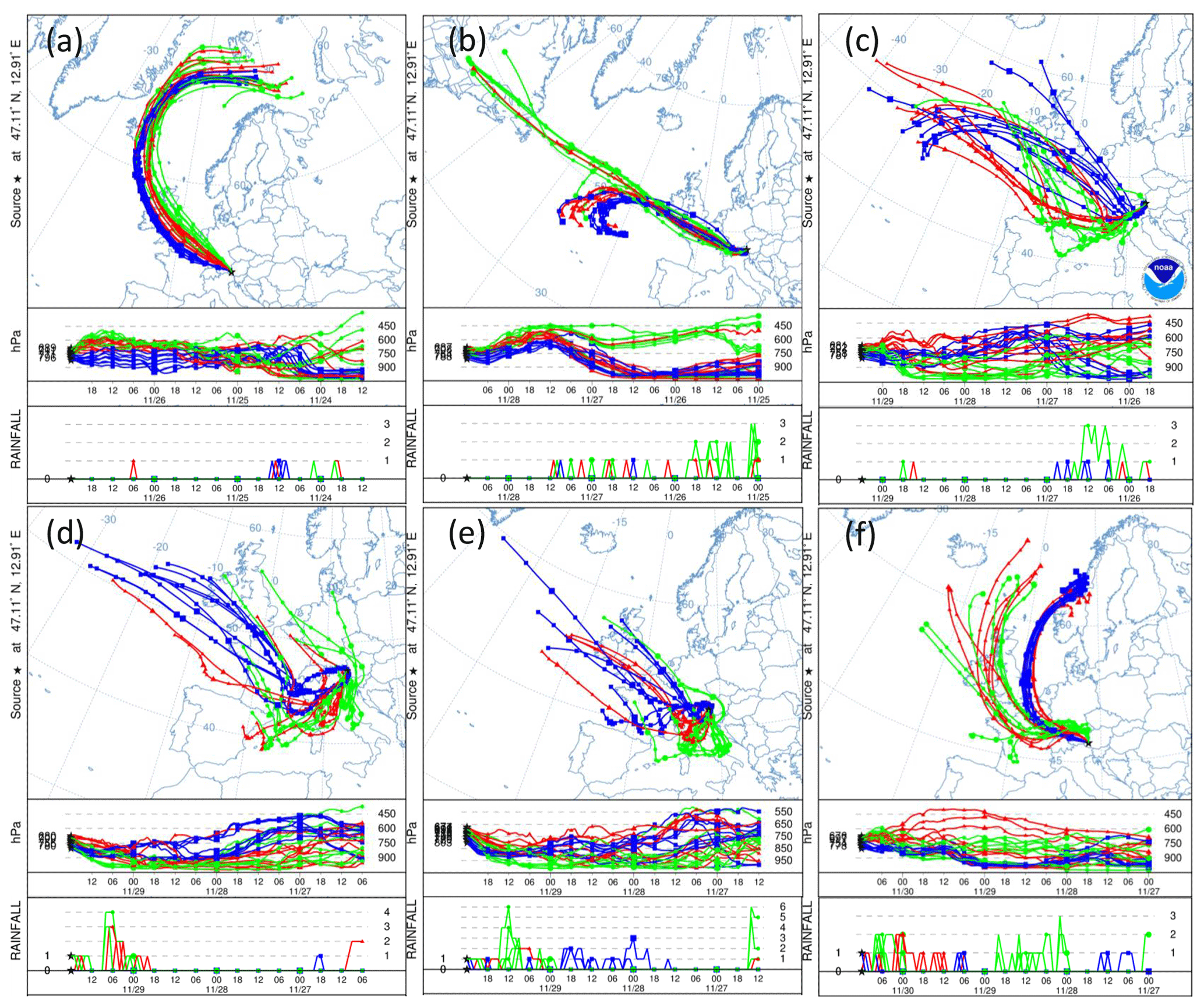
Figure A8(a) 84 h HYSPLIT back trajectories from the Sonnblick Observatory, initialized at 00:00 UTC on 27 November, (b) 12:00 UTC on 28 November, (c) 06:00 UTC and (d) 18:00 UTC on 29 November, and (e) 00:00 UTC and (f) 12:00 UTC on 30 November. The blue, green and red lines represent eight ensemble back trajectories initialized 1000, 2000 and 3000 m above the model terrain height, respectively. The two lower panels in each subplot show the back trajectory height in units of pressure (hPa) and rainfall (mm) as a function of time (in 6-hourly intervals) and as a function of pressure (in hPa).
DRINCZ was developed and designed by ROD, with the assistance of MCC, MR, LSB, KPB and NBD. The SA water experiments were conducted by MCC, KPB, LSB, VW, JW, SB and ROD. The temperature calibration and NX-illite experiments were conducted and analyzed by KPB and NBD. The snow samples were collected by NE and analyzed by ROD. The instrumental error, uncertainties and calibration were conducted by ROD, with contributions from ZAK and CM. The automation and analysis software was developed by ROD, with contributions from KPB and MCC. The well plate holder was designed by MR and ROD and manufactured by MR. The paper was written by ROD, with contributions from NBD, CM and ZAK. The project was supervised by ZAK.
The authors declare that they have no conflict of interest.
Zamin A. Kanji would like to acknowledge Franz Conen and Emillano Stopelli for assistance with the initial set up of the droplet freezing assay. We are grateful to James D. Atkinson for discussions and help with experiments during the preparatory phase of DRINCZ development. We acknowledge technical assistance from Hannes Wylder. Robert O. David would like to thank William Ball for insightful statistical discussions, Ellen Gute for performing camera tests and Michele Gregorini for assistance with the automation.
This research has been supported by the Swiss National Science Foundation (grant no. 200021_156581).
This paper was edited by Pierre Herckes and reviewed by Gabor Vali and one anonymous referee.
Ansmann, A., Tesche, M., Seifert, P., Althausen, D., Engelmann, R., Fruntke, J., Wandinger, U., Mattis, I., and Müller, D.: Evolution of the ice phase in tropical altocumulus: SAMUM lidar observations over Cape Verde, J. Geophys. Res., 114, D17208, https://doi.org/10.1029/2008JD011659, 2009.
Atherton, T. J. and Kerbyson, D. J.: Size Invariant Circle Detection, Image Vision Comput., 17, 795–803, 1999.
Atkinson, J. D., Murray, B. J., Woodhouse, M. T., Whale, T. F., Baustian, K. J., Carslaw, K. S., Dobbie, S., O'Sullivan, D., and Malkin, T. L.: The importance of feldspar for ice nucleation by mineral dust in mixed-phase clouds, Nature, 498, 355–358, https://doi.org/10.1038/nature12278, 2013.
Ault, A. P., Williams, C. R., White, A. B., Neiman, P. J., Creamean, J. M., Gaston, C. J., Ralph, F. M., and Prather, K. A.: Detection of Asian dust in California orographic precipitation, J. Geophys. Res., 116, D16205, https://doi.org/10.1029/2010JD015351, 2011.
Beall, C. M., Stokes, M. D., Hill, T. C., DeMott, P. J., DeWald, J. T., and Prather, K. A.: Automation and heat transfer characterization of immersion mode spectroscopy for analysis of ice nucleating particles, Atmos. Meas. Tech., 10, 2613–2626, https://doi.org/10.5194/amt-10-2613-2017, 2017.
Beck, A., Henneberger, J., Fugal, J. P., David, R. O., Lacher, L., and Lohmann, U.: Impact of surface and near-surface processes on ice crystal concentrations measured at mountain-top research stations, Atmos. Chem. Phys., 18, 8909–8927, https://doi.org/10.5194/acp-18-8909-2018, 2018.
de Boer, G., Morrison, H., Shupe, M. D., and Hildner, R.: Evidence of liquid dependent ice nucleation in high-latitude stratiform clouds from surface remote sensors, Geophys. Res. Lett., 38, L01803, https://doi.org/10.1029/2010GL046016, 2011.
Boose, Y., Welti, A., Atkinson, J., Ramelli, F., Danielczok, A., Bingemer, H. G., Plötze, M., Sierau, B., Kanji, Z. A., and Lohmann, U.: Heterogeneous ice nucleation on dust particles sourced from nine deserts worldwide – Part 1: Immersion freezing, Atmos. Chem. Phys., 16, 15075–15095, https://doi.org/10.5194/acp-16-15075-2016, 2016a.
Boose, Y., Kanji, Z. A., Kohn, M., Sierau, B., Zipori, A., Crawford, I., Lloyd, G., Bukowiecki, N., Herrmann, E., Kupiszewski, P., Steinbacher, M., and Lohmann, U.: Ice Nucleating Particle Measurements at 241 K during Winter Months at 3580 m MSL in the Swiss Alps, J. Atmos. Sci., 73, 2203–2228, https://doi.org/10.1175/JAS-D-15-0236.1, 2016b.
Broadley, S. L., Murray, B. J., Herbert, R. J., Atkinson, J. D., Dobbie, S., Malkin, T. L., Condliffe, E., and Neve, L.: Immersion mode heterogeneous ice nucleation by an illite rich powder representative of atmospheric mineral dust, Atmos. Chem. Phys., 12, 287–307, https://doi.org/10.5194/acp-12-287-2012, 2012.
Burkert-Kohn, M., Wex, H., Welti, A., Hartmann, S., Grawe, S., Hellner, L., Herenz, P., Atkinson, J. D., Stratmann, F., and Kanji, Z. A.: Leipzig Ice Nucleation chamber Comparison (LINC): intercomparison of four online ice nucleation counters, Atmos. Chem. Phys., 17, 11683–11705, https://doi.org/10.5194/acp-17-11683-2017, 2017.
Christner, B. C., Cai, R., Morris, C. E., McCarter, K. S., Foreman, C. M., Skidmore, M. L., Montross, S. N., and Sands, D. C.: Geographic, seasonal, and precipitation chemistry influence on the abundance and activity of biological ice nucleators in rain and snow, P. Natl. Acad. Sci. USA, 105, 18854–18859, https://doi.org/10.1073/pnas.0809816105, 2008.
Creamean, J. M., Suski, K. J., Rosenfeld, D., Cazorla, A., DeMott, P. J., Sullivan, R. C., White, A. B., Ralph, F. M., Minnis, P., Comstock, J. M., Tomlinson, J. M., and Prather, K. A.: Dust and Biological Aerosols from the Sahara and Asia Influence Precipitation in the Western U.S., Science, 339, 1572–1578, https://doi.org/10.1126/science.1227279, 2013.
Cziczo, D. J., Ladino, L., Boose, Y., Kanji, Z. A., Kupiszewski, P., Lance, S., Mertes, S., and Wex, H.: Measurements of Ice Nucleating Particles and Ice Residuals, Meteor. Mon., 58, 8.1–8.13, https://doi.org/10.1175/AMSMONOGRAPHS-D-16-0008.1, 2017.
David, R. O., Cascajo Castresana, M., Brennan, K. P., Rösch, M., Els, N., Werz, J., Weichlinger, V., Boynton, L. S., Bogler, S., Borduas-Dedekind, N., Marcolli, C., and Kanji, Z. A.: Development of the DRoplet Ice Nuclei Counter Zürich (DRINCZ): Validation and application to field collected snow samples, https://doi.org/10.3929/ethz-b-000369839, 2019.
DeMott, P. J., Cziczo, D. J., Prenni, A. J., Murphy, D. M., Kreidenweis, S. M., Thomson, D. S., Borys, R., and Rogers, D. C.: Measurements of the concentration and composition of nuclei for cirrus formation, P. Natl. Acad. Sci. USA, 100, 14655–14660, https://doi.org/10.1073/pnas.2532677100, 2003.
DeMott, P. J., Prenni, A. J., McMeeking, G. R., Sullivan, R. C., Petters, M. D., Tobo, Y., Niemand, M., Möhler, O., Snider, J. R., Wang, Z., and Kreidenweis, S. M.: Integrating laboratory and field data to quantify the immersion freezing ice nucleation activity of mineral dust particles, Atmos. Chem. Phys., 15, 393–409, https://doi.org/10.5194/acp-15-393-2015, 2015.
DeMott, P. J., Hill, T. C. J., McCluskey, C. S., Prather, K. A., Collins, D. B., Sullivan, R. C., Ruppel, M. J., Mason, R. H., Irish, V. E., Lee, T., Hwang, C. Y., Rhee, T. S., Snider, J. R., McMeeking, G. R., Dhaniyala, S., Lewis, E. R., Wentzell, J. J. B., Abbatt, J., Lee, C., Sultana, C. M., Ault, A. P., Axson, J. L., Martinez, M. D., Venero, I., Santos-Figueroa, G., Stokes, M. D., Deane, G. B., Mayol-Bracero, O. L., Grassian, V. H., Bertram, T. H., Bertram, A. K., Moffett, B. F., and Franc, G. D.: Sea spray aerosol as a unique source of ice nucleating particles, P. Natl. Acad. Sci. USA, 113, 5797–5803, https://doi.org/10.1073/pnas.1514034112, 2016.
DeMott, P. J., Hill, T. C. J., Petters, M. D., Bertram, A. K., Tobo, Y., Mason, R. H., Suski, K. J., McCluskey, C. S., Levin, E. J. T., Schill, G. P., Boose, Y., Rauker, A. M., Miller, A. J., Zaragoza, J., Rocci, K., Rothfuss, N. E., Taylor, H. P., Hader, J. D., Chou, C., Huffman, J. A., Pöschl, U., Prenni, A. J., and Kreidenweis, S. M.: Comparative measurements of ambient atmospheric concentrations of ice nucleating particles using multiple immersion freezing methods and a continuous flow diffusion chamber, Atmos. Chem. Phys., 17, 11227–11245, https://doi.org/10.5194/acp-17-11227-2017, 2017.
Derrick, B. and White, P.: Why Welch's test is Type I error robust, The Quantitative Methodsfor Psychology, 12, 30–38, https://doi.org/10.20982/tqmp.12.1.p030, 2016.
Felgitsch, L., Baloh, P., Burkart, J., Mayr, M., Momken, M. E., Seifried, T. M., Winkler, P., Schmale III, D. G., and Grothe, H.: Birch leaves and branches as a source of ice-nucleating macromolecules, Atmos. Chem. Phys., 18, 16063–16079, https://doi.org/10.5194/acp-18-16063-2018, 2018.
Field, P. R., Möhler, O., Connolly, P., Krämer, M., Cotton, R., Heymsfield, A. J., Saathoff, H., and Schnaiter, M.: Some ice nucleation characteristics of Asian and Saharan desert dust, Atmos. Chem. Phys., 6, 2991–3006, https://doi.org/10.5194/acp-6-2991-2006, 2006.
Fletcher, N. H.: The physics of rainclouds, Cambridge University Press, New York, USA, 1962.
Harrison, A. D., Whale, T. F., Rutledge, R., Lamb, S., Tarn, M. D., Porter, G. C. E., Adams, M. P., McQuaid, J. B., Morris, G. J., and Murray, B. J.: An instrument for quantifying heterogeneous ice nucleation in multiwell plates using infrared emissions to detect freezing, Atmos. Meas. Tech., 11, 5629–5641, https://doi.org/10.5194/amt-11-5629-2018, 2018.
Hartmann, S., Niedermeier, D., Voigtländer, J., Clauss, T., Shaw, R. A., Wex, H., Kiselev, A., and Stratmann, F.: Homogeneous and heterogeneous ice nucleation at LACIS: operating principle and theoretical studies, Atmos. Chem. Phys., 11, 1753–1767, https://doi.org/10.5194/acp-11-1753-2011, 2011.
Hill, T. C. J., Moffett, B. F., DeMott, P. J., Georgakopoulos, D. G., Stump, W. L., and Franc, G. D.: Measurement of Ice Nucleation-Active Bacteria on Plants and in Precipitation by Quantitative PCR, Appl. Environ. Microb., 80, 1256–1267, https://doi.org/10.1128/AEM.02967-13, 2014.
Hiranuma, N., Augustin-Bauditz, S., Bingemer, H., Budke, C., Curtius, J., Danielczok, A., Diehl, K., Dreischmeier, K., Ebert, M., Frank, F., Hoffmann, N., Kandler, K., Kiselev, A., Koop, T., Leisner, T., Möhler, O., Nillius, B., Peckhaus, A., Rose, D., Weinbruch, S., Wex, H., Boose, Y., DeMott, P. J., Hader, J. D., Hill, T. C. J., Kanji, Z. A., Kulkarni, G., Levin, E. J. T., McCluskey, C. S., Murakami, M., Murray, B. J., Niedermeier, D., Petters, M. D., O'Sullivan, D., Saito, A., Schill, G. P., Tajiri, T., Tolbert, M. A., Welti, A., Whale, T. F., Wright, T. P., and Yamashita, K.: A comprehensive laboratory study on the immersion freezing behavior of illite NX particles: a comparison of 17 ice nucleation measurement techniques, Atmos. Chem. Phys., 15, 2489–2518, https://doi.org/10.5194/acp-15-2489-2015, 2015.
Hiranuma, N., Adachi, K., Bell, D. M., Belosi, F., Beydoun, H., Bhaduri, B., Bingemer, H., Budke, C., Clemen, H.-C., Conen, F., Cory, K. M., Curtius, J., DeMott, P. J., Eppers, O., Grawe, S., Hartmann, S., Hoffmann, N., Höhler, K., Jantsch, E., Kiselev, A., Koop, T., Kulkarni, G., Mayer, A., Murakami, M., Murray, B. J., Nicosia, A., Petters, M. D., Piazza, M., Polen, M., Reicher, N., Rudich, Y., Saito, A., Santachiara, G., Schiebel, T., Schill, G. P., Schneider, J., Segev, L., Stopelli, E., Sullivan, R. C., Suski, K., Szakáll, M., Tajiri, T., Taylor, H., Tobo, Y., Ullrich, R., Weber, D., Wex, H., Whale, T. F., Whiteside, C. L., Yamashita, K., Zelenyuk, A., and Möhler, O.: A comprehensive characterization of ice nucleation by three different types of cellulose particles immersed in water, Atmos. Chem. Phys., 19, 4823–4849, https://doi.org/10.5194/acp-19-4823-2019, 2019.
Hoose, C. and Möhler, O.: Heterogeneous ice nucleation on atmospheric aerosols: a review of results from laboratory experiments, Atmos. Chem. Phys., 12, 9817–9854, https://doi.org/10.5194/acp-12-9817-2012, 2012.
Irish, V. E., Elizondo, P., Chen, J., Chou, C., Charette, J., Lizotte, M., Ladino, L. A., Wilson, T. W., Gosselin, M., Murray, B. J., Polishchuk, E., Abbatt, J. P. D., Miller, L. A., and Bertram, A. K.: Ice-nucleating particles in Canadian Arctic sea-surface microlayer and bulk seawater, Atmos. Chem. Phys., 17, 10583–10595, https://doi.org/10.5194/acp-17-10583-2017, 2017.
Kanji, Z. A., Ladino, L. A., Wex, H., Boose, Y., Burkert-Kohn, M., Cziczo, D. J., and Krämer, M.: Overview of Ice Nucleating Particles, Meteor. Mon., 58, 1.1–1.33, https://doi.org/10.1175/AMSMONOGRAPHS-D-16-0006.1, 2017.
Kaufmann, L., Marcolli, C., Hofer, J., Pinti, V., Hoyle, C. R., and Peter, T.: Ice nucleation efficiency of natural dust samples in the immersion mode, Atmos. Chem. Phys., 16, 11177–11206, https://doi.org/10.5194/acp-16-11177-2016, 2016.
Kohn, M., Lohmann, U., Welti, A., and Kanji, Z. A.: Immersion mode ice nucleation measurements with the new Portable Immersion Mode Cooling chAmber (PIMCA), J. Geophys. Res.-Atmos., 121, 4713–4733, https://doi.org/10.1002/2016JD024761, 2016.
Lacher, L., Lohmann, U., Boose, Y., Zipori, A., Herrmann, E., Bukowiecki, N., Steinbacher, M., and Kanji, Z. A.: The Horizontal Ice Nucleation Chamber (HINC): INP measurements at conditions relevant for mixed-phase clouds at the High Altitude Research Station Jungfraujoch, Atmos. Chem. Phys., 17, 15199–15224, https://doi.org/10.5194/acp-17-15199-2017, 2017.
Lacher, L., Steinbacher, M., Bukowiecki, N., Herrmann, E., Zipori, A., and Kanji, Z. A.: Impact of Air Mass Conditions and Aerosol Properties on Ice Nucleating Particle Concentrations at the High Altitude Research Station Jungfraujoch, Atmosphere, 9, 363, https://doi.org/10.3390/atmos9090363, 2018.
Lohmann, U. and Feichter, J.: Global indirect aerosol effects: a review, Atmos. Chem. Phys., 5, 715–737, https://doi.org/10.5194/acp-5-715-2005, 2005.
Lowenthal, D., Hallar, A. G., McCubbin, I., David, R., Borys, R., Blossey, P., Muhlbauer, A., Kuang, Z., and Moore, M.: Isotopic Fractionation in Wintertime Orographic Clouds, J. Atmos. Ocean. Tech., 33, 2663–2678, https://doi.org/10.1175/JTECH-D-15-0233.1, 2016.
Lüönd, F., Stetzer, O., Welti, A., and Lohmann, U.: Experimental study on the ice nucleation ability of size-selected kaolinite particles in the immersion mode, J. Geophys. Res., 115, D14201, https://doi.org/10.1029/2009JD012959, 2010.
Marcolli, C., Gedamke, S., Peter, T., and Zobrist, B.: Efficiency of immersion mode ice nucleation on surrogates of mineral dust, Atmos. Chem. Phys., 7, 5081–5091, https://doi.org/10.5194/acp-7-5081-2007, 2007.
Matus, A. V. and L'Ecuyer, T. S.: The role of cloud phase in Earth's radiation budget, J. Geophys. Res.-Atmos., 122, 2559–2578, https://doi.org/10.1002/2016JD025951, 2017.
McCluskey, C. S., Ovadnevaite, J., Rinaldi, M., Atkinson, J., Belosi, F., Ceburnis, D., Marullo, S., Hill, T. C. J., Lohmann, U., Kanji, Z. A., O'Dowd, C., Kreidenweis, S. M., and DeMott, P. J.: Marine and Terrestrial Organic Ice-Nucleating Particles in Pristine Marine to Continentally Influenced Northeast Atlantic Air Masses, J. Geophys. Res.-Atmos., 123, 6196–6212, https://doi.org/10.1029/2017JD028033, 2018.
Mülmenstädt, J., Sourdeval, O., Delanoë, J., and Quaas, J.: Frequency of occurrence of rain from liquid-, mixed-, and ice-phase clouds derived from A-Train satellite retrievals: RAIN FROM LIQUID- AND ICE-PHASE CLOUDS, Geophys. Res. Lett., 42, 6502–6509, https://doi.org/10.1002/2015GL064604, 2015.
Murray, B. J., Broadley, S. L., Wilson, T. W., Bull, S. J., Wills, R. H., Christenson, H. K., and Murray, E. J.: Kinetics of the homogeneous freezing of water, Phys. Chem. Chem. Phys., 12, 10380–10387, https://doi.org/10.1039/C003297B, 2010.
Murray, B. J., O'Sullivan, D., Atkinson, J. D., and Webb, M. E.: Ice nucleation by particles immersed in supercooled cloud droplets, Chem. Soc. Rev., 41, 6519–6554, https://doi.org/10.1039/C2CS35200A, 2012.
Niemand, M., Möhler, O., Vogel, B., Vogel, H., Hoose, C., Connolly, P., Klein, H., Bingemer, H., DeMott, P., Skrotzki, J., and Leisner, T.: A Particle-Surface-Area-Based Parameterization of Immersion Freezing on Desert Dust Particles, J. Atmos. Sci., 69, 3077–3092, https://doi.org/10.1175/JAS-D-11-0249.1, 2012.
Petters, M. D. and Wright, T. P.: Revisiting ice nucleation from precipitation samples, Geophys. Res. Lett., 42, 8758–8766, https://doi.org/10.1002/2015GL065733, 2015.
Pinti, V., Marcolli, C., Zobrist, B., Hoyle, C. R., and Peter, T.: Ice nucleation efficiency of clay minerals in the immersion mode, Atmos. Chem. Phys., 12, 5859–5878, https://doi.org/10.5194/acp-12-5859-2012, 2012.
Polen, M., Brubaker, T., Somers, J., and Sullivan, R. C.: Cleaning up our water: reducing interferences from nonhomogeneous freezing of “pure” water in droplet freezing assays of ice-nucleating particles, Atmos. Meas. Tech., 11, 5315–5334, https://doi.org/10.5194/amt-11-5315-2018, 2018.
Pummer, B. G., Bauer, H., Bernardi, J., Bleicher, S., and Grothe, H.: Suspendable macromolecules are responsible for ice nucleation activity of birch and conifer pollen, Atmos. Chem. Phys., 12, 2541–2550, https://doi.org/10.5194/acp-12-2541-2012, 2012.
Puxbaum, H. and Tscherwenka, W.: Relationships of major ions in snow fall and rime at sonnblick observatory (SBO, 3106 m) and implications for scavenging processes in mixed clouds, Atmos. Environ., 32, 4011–4020, https://doi.org/10.1016/S1352-2310(98)00244-1, 1998.
Reicher, N., Segev, L., and Rudich, Y.: The WeIzmann Supercooled Droplets Observation on a Microarray (WISDOM) and application for ambient dust, Atmos. Meas. Tech., 11, 233–248, https://doi.org/10.5194/amt-11-233-2018, 2018.
Richardson, M. S., DeMott, P. J., Kreidenweis, S. M., Cziczo, D. J., Dunlea, E. J., Jimenez, J. L., Thomson, D. S., Ashbaugh, L. L., Borys, R. D., Westphal, D. L., Casuccio, G. S., and Lersch, T. L.: Measurements of heterogeneous ice nuclei in the western United States in springtime and their relation to aerosol characteristics, J. Geophys. Res., 112, D02209, https://doi.org/10.1029/2006JD007500, 2007.
Riechers, B., Wittbracht, F., Hütten, A., and Koop, T.: The homogeneous ice nucleation rate of water droplets produced in a microfluidic device and the role of temperature uncertainty, Phys. Chem. Chem. Phys., 15, 5873, https://doi.org/10.1039/c3cp42437e, 2013.
Roebber, P. J., Bruening, S. L., Schultz, D. M., and Cortinas, J. V.: Improving Snowfall Forecasting by Diagnosing Snow Density, Weather Forecast., 18, 264–287, https://doi.org/10.1175/1520-0434(2003)018<0264:ISFBDS>2.0.CO;2, 2003.
Rogers, D. C.: Development of a continuous flow thermal gradient diffusion chamber for ice nucleation studies, Atmos. Res., 22, 149–181, https://doi.org/10.1016/0169-8095(88)90005-1, 1988.
Rolph, G., Stein, A., and Stunder, B.: Real-time Environmental Applications and Display sYstem: READY, Environ. Model. Softw., 95, 210–228, https://doi.org/10.1016/j.envsoft.2017.06.025, 2017.
Spiess, A.-N., Feig, C., and Ritz, C.: Highly accurate sigmoidal fitting of real-time PCR data by introducing a parameter for asymmetry, BMC Bioinformatics, 9, 221, https://doi.org/10.1186/1471-2105-9-221, 2008.
Stan, C. A., Schneider, G. F., Shevkoplyas, S. S., Hashimoto, M., Ibanescu, M., Wiley, B. J., and Whitesides, G. M.: A microfluidic apparatus for the study of ice nucleation in supercooled water drops, Lab. Chip, 9, 2293–2305, https://doi.org/10.1039/B906198C, 2009.
Stein, A. F., Draxler, R. R., Rolph, G. D., Stunder, B. J. B., Cohen, M. D., and Ngan, F.: NOAA's HYSPLIT Atmospheric Transport and Dispersion Modeling System, B. Am. Meteorol. Soc., 96, 2059–2077, https://doi.org/10.1175/BAMS-D-14-00110.1, 2015.
Stetzer, O., Baschek, B., Lüönd, F., and Lohmann, U.: The Zurich Ice Nucleation Chamber (ZINC)-A New Instrument to Investigate Atmospheric Ice Formation, Aerosol Sci. Tech., 42, 64–74, https://doi.org/10.1080/02786820701787944, 2008.
Stopelli, E., Conen, F., Zimmermann, L., Alewell, C., and Morris, C. E.: Freezing nucleation apparatus puts new slant on study of biological ice nucleators in precipitation, Atmos. Meas. Tech., 7, 129–134, https://doi.org/10.5194/amt-7-129-2014, 2014.
Stopelli, E., Conen, F., Morris, C. E., Herrmann, E., Bukowiecki, N., and Alewell, C.: Ice nucleation active particles are efficiently removed by precipitating clouds, Scientific Reports, 5, 16433, https://doi.org/10.1038/srep16433, 2015.
Tan, I., Storelvmo, T., and Zelinka, M. D.: Observational constraints on mixed-phase clouds imply higher climate sensitivity, Science, 352, 224–227, https://doi.org/10.1126/science.aad5300, 2016.
Tarn, M. D., Sikora, S. N. F., Porter, G. C. E., O'Sullivan, D., Adams, M., Whale, T. F., Harrison, A. D., Vergara-Temprado, J., Wilson, T. W., Shim, J., and Murray, B. J.: The study of atmospheric ice-nucleating particles via microfluidically generated droplets, Microfluid. Nanofluid., 22, 52 https://doi.org/10.1007/s10404-018-2069-x, 2018.
Vali, G.: Quantitative Evaluation of Experimental Results an the Heterogeneous Freezing Nucleation of Supercooled Liquids, J. Atmos. Sci., 28, 402–409, https://doi.org/10.1175/1520-0469(1971)028<0402:QEOERA>2.0.CO;2, 1971.
Vali, G.: Revisiting the differential freezing nucleus spectra derived from drop-freezing experiments: methods of calculation, applications, and confidence limits, Atmos. Meas. Tech., 12, 1219–1231, https://doi.org/10.5194/amt-12-1219-2019, 2019.
Vali, G. and Upper, C. D.: Principles of Ice Nucleation, in: Biological Ice Nucleation and Its Applications, edited by: Lee, R. E., Warren, G. J., and Gusta, L. V., The American Phytopathological Society, St. Paul, Minnesota, USA, available at: https://www.loot.co.za/product/richard-e-lee-biological-ice-nucleation-and-its-applica/wxrm-421-gaa0 (last access: 16 September 2019), 1995.
Vali, G., DeMott, P. J., Möhler, O., and Whale, T. F.: Technical Note: A proposal for ice nucleation terminology, Atmos. Chem. Phys., 15, 10263–10270, https://doi.org/10.5194/acp-15-10263-2015, 2015.
Welti, A., Müller, K., Fleming, Z. L., and Stratmann, F.: Concentration and variability of ice nuclei in the subtropical maritime boundary layer, Atmos. Chem. Phys., 18, 5307–5320, https://doi.org/10.5194/acp-18-5307-2018, 2018.
Westbrook, C. D. and Illingworth, A. J.: Evidence that ice forms primarily in supercooled liquid clouds at temperatures ∘C, Geophys. Res. Lett., 38, L14808, https://doi.org/10.1029/2011GL048021, 2011.
Wex, H., Augustin-Bauditz, S., Boose, Y., Budke, C., Curtius, J., Diehl, K., Dreyer, A., Frank, F., Hartmann, S., Hiranuma, N., Jantsch, E., Kanji, Z. A., Kiselev, A., Koop, T., Möhler, O., Niedermeier, D., Nillius, B., Rösch, M., Rose, D., Schmidt, C., Steinke, I., and Stratmann, F.: Intercomparing different devices for the investigation of ice nucleating particles using Snomax® as test substance, Atmos. Chem. Phys., 15, 1463–1485, https://doi.org/10.5194/acp-15-1463-2015, 2015.
Wex, H., Huang, L., Zhang, W., Hung, H., Traversi, R., Becagli, S., Sheesley, R. J., Moffett, C. E., Barrett, T. E., Bossi, R., Skov, H., Hünerbein, A., Lubitz, J., Löffler, M., Linke, O., Hartmann, M., Herenz, P., and Stratmann, F.: Annual variability of ice-nucleating particle concentrations at different Arctic locations, Atmos. Chem. Phys., 19, 5293–5311, https://doi.org/10.5194/acp-19-5293-2019, 2019.
Whale, T. F., Murray, B. J., O'Sullivan, D., Wilson, T. W., Umo, N. S., Baustian, K. J., Atkinson, J. D., Workneh, D. A., and Morris, G. J.: A technique for quantifying heterogeneous ice nucleation in microlitre supercooled water droplets, Atmos. Meas. Tech., 8, 2437–2447, https://doi.org/10.5194/amt-8-2437-2015, 2015.
Wilson, T. W., Ladino, L. A., Alpert, P. A., Breckels, M. N., Brooks, I. M., Browse, J., Burrows, S. M., Carslaw, K. S., Huffman, J. A., Judd, C., Kilthau, W. P., Mason, R. H., McFiggans, G., Miller, L. A., Nájera, J. J., Polishchuk, E., Rae, S., Schiller, C. L., Si, M., Temprado, J. V., Whale, T. F., Wong, J. P. S., Wurl, O., Yakobi-Hancock, J. D., Abbatt, J. P. D., Aller, J. Y., Bertram, A. K., Knopf, D. A., and Murray, B. J.: A marine biogenic source of atmospheric ice-nucleating particles, Nature, 525, 234–238, https://doi.org/10.1038/nature14986, 2015.