3-D tomographic limb sounder retrieval techniques: irregular grids and Laplacian regularisation

Multiple limb sounder measurements of the same atmospheric region taken from different directions can be combined in a 3-D tomographic retrieval. Mathematically, this is a computationally expensive inverse modelling problem. It typically requires an introduction of some general knowledge of the atmosphere (regularisation) due to its underdetermined nature.

This paper introduces a consistent, physically motivated (no ad-hoc parameters) variant of the Tikhonov regularisation scheme based on spatial derivatives of the first-order and Laplacian. As shown by a case study with synthetic data, this scheme, combined with irregular grid retrieval methods employing Delaunay triangulation, improves both upon the quality and the computational cost of 3-D tomography. It also eliminates grid dependence and the need to tune parameters for each use case. The few physical parameters required can be derived from in situ measurements and model data. Tests show that a 82 % reduction in the number of grid points and 50 % reduction in total computation time, compared to previous methods, could be achieved without compromising results. An efficient Monte Carlo technique was also adopted for accuracy estimation of the new retrievals.

1 Introduction

Dynamics and mixing processes in the upper troposphere and lower stratosphere (UTLS) are of great interest. They control the exchange between these layers (Gettelman et al., 2011) and have a strong influence on the composition and thereby on radiative forcing (Forster and Shine, 1997; Riese et al., 2012). High spatial resolution observations are required to understand the low length-scale processes typical of this region.

Infrared limb sounding is an important tool for measuring the temperature and volume mixing ratios of trace gases in UTLS with high resolution, especially in the vertical direction, which is critical for resolving typical structures there (e.g. Birner, 2006; Hegglin et al., 2009). Modern limb sounders are capable of high-frequency operation, resulting in many measurements that are taken close to one another, which are best exploited if the data from these measurements can be combined. Producing a 2-D curtain of an atmosphere along the flight path of the instrument by combining the observations close to each other is already an established technique (e.g. Steck et al., 2005; Worden et al., 2004). With suitable measurement geometries, this technique can be extended to obtain 3-D data.

A tomographic data retrieval uses multiple measurements of the same air mass, taken from different directions, to obtain high-resolution 3-D temperature and trace gas concentration data. There is, as it often happens with remote sensing retrievals, a large number of the atmospheric states that would agree with the given observations within their expected precision. A regularisation algorithm is employed to pick the solution that is in best agreement with our prior knowledge of the atmospheric state and general understanding of the physics involved. The mathematical framework of the tomographic retrieval is outlined in Sect. 2.1.

The classic Tikhonov regularisation scheme (Tikhonov and Arsenin, 1977) is an established technique used for infrared limb sounding instruments such as the Michelson Interferometer for Passive Atmospheric Sounding (Steck et al., 2005; Carlotti et al., 2001), and GLORIA (Ungermann et al., 2010; Ungermann et al., 2011). It quantifies the spatial continuity of an atmospheric state by evaluating spatial derivatives of the retrieved quantities. This technique serves the purpose of ruling out very pathological, oscillatory retrieval results, but requires fine tuning of several unphysical ad-hoc parameters and subsequent validation. In this paper, we introduce an improved, more physically and statistically motivated approach to regularisation that requires less tuning. It relies on the calculation of both the derivatives of the first order and Laplacian of atmospheric quantities, which provide more complete information about smoothness and feasibility of a particular atmospheric state. The regularisation parameters we use are physical, in the sense that they can be estimated from in situ measurements or model data and are less grid dependent: their values, once established, can be more readily used for new retrievals.

Data retrievals from limb sounders are typically performed on a rectilinear grid. In this paper, we define a rectilinear grid by taking a set of longitudes, a set of latitudes and a set of altitudes and placing a grid point at each of the possible combinations of these coordinates. Such grids can be a limiting factor for efficiency of numerical calculations. Due to the exponential nature of atmosphere density distribution with altitude, most of the radiance along any line of sight of a limb imager comes from the vicinity of the lowest altitude point on a given line of sight (called the “tangent point”). The resolution of the retrieved data depends on the density of tangent points in the area. For airborne observations this density is highly inhomogeneous. The densely measured regions are limited in size, located below flight altitude only and rarely rectangular. The large, poorly resolved areas with little or no tangent points still need to be included in the grid as long as lines of sight of any measurements pass through them. A rectilinear grid retrieval tends to either underresolve the well-measured area, or waste memory and computation time for regions with few measurements. To avoid this problem, a tomographic retrieval on an irregular grid with Delaunay triangulation was developed (Sect. 2). It allows for significant computational cost improvements without compromising retrieval quality.

Most retrieval error estimation techniques would be unreasonably computationally expensive in the case of a 3-D tomographic retrieval. Monte Carlo methods allow a relatively quick error estimation. In order to apply Monte Carlo for a 3-D tomographic retrieval on an irregular grid and using our newly developed regularisation, dedicated algorithms have to be developed. These are presented in Sect. 3.

The new methods described in Sects. 2 and 3 were tested with synthetic measurement data to compare their results and computational costs. The tests, and their results, are described in detail in Sect. 4.

2 Regularisation improvements and irregular grids

2.1 The retrieval

The main focus of this paper is the algorithm for retrieving atmospheric quantities, such as temperature or trace gas mixing ratios, from limb sounder measurements in 3-D. In this section, we outline the general inverse modelling approach to this problem and identify some aspects we aim to improve upon.

Let an atmospheric state vector x∈ℝⁿ represent the values of some atmospheric quantities on a finite grid and let y∈ℝ^m be a set of m remote measurements taken within the region in question. The physics of the measurement process itself has to be understood for the instrument to be practical, so one can usually build a theoretical model of the measurement (the forward model) $F:{\mathbb{R}}^n\to {\mathbb{R}}^m$. The inverse problem of determining x given y is then typically both underdetermined and ill posed: many atmospheric states would result in the same measurement, but due to instrument and model errors no states would yield the exact measurement result y. One can solve this problem by finding an atmospheric state x that minimises the following quadratic cost function:

$$\begin{array}{ll}{\displaystyle }& {\displaystyle }J\left(\mathit{x}\right)={\left(\mathit{F}\left(\mathit{x}\right)-\mathit{y}\right)}^T{\mathbf{S}}_{\mathit{ϵ}}^{-\mathrm{1}}\left(\mathit{F}\left(\mathit{x}\right)-\mathit{y}\right)\\ \text{(1)}& {\displaystyle }& {\displaystyle }+{\left(\mathit{x}-{\mathit{x}}_{\mathrm{a}}\right)}^T{\mathbf{S}}_{\mathrm{a}}^{-\mathrm{1}}\left(\mathit{x}-{\mathit{x}}_{\mathrm{a}}\right).\end{array}$$

The first term of Eq. (1) quantifies the difference between the actual measurement and a simulated one (given the atmospheric state is x). The matrix ${\mathbf{S}}_{\mathit{ϵ}}^{-\mathrm{1}}\in {\mathbb{R}}^m\times {\mathbb{R}}^m$ represents the expected instrument errors. The second term introduces regularisation; i.e. it is larger for x that are unlikely given our general, measurement-unrelated knowledge about the atmosphere. In practice this is achieved using an a priori state x_a, usually derived from climatologies. It is meant for introducing the best of our prior knowledge into the retrieval process without imposing any features of the kind to be measured. The precision matrix ${\mathbf{S}}_{\mathrm{a}}^{-\mathrm{1}}$ (the inverse of a covariance matrix for atmospheric states S_a) contains prior knowledge about the probability distribution of atmospheric states. For a more detailed discussion of this approach refer to Rodgers (2000).

Finding the precision matrix ${\mathbf{S}}_{\mathrm{a}}^{-\mathrm{1}}$ that would correctly represent the physical and statistical properties of the atmosphere is challenging. The Tikhonov regularisation approach (Tikhonov and Arsenin, 1977)

$$\begin{array}{}\text{(2)}& {\mathbf{S}}_{\mathrm{a}}^{-\mathrm{1}}={\mathit{\alpha }}_{\mathrm{0}}^{\mathrm{2}}{\mathbf{L}}_{\mathrm{0}}{\mathbf{L}}_{\mathrm{0}}^T+{\mathit{\alpha }}_v^{\mathrm{2}}{\mathbf{L}}_z{\mathbf{L}}_z^T+{\mathit{\alpha }}_h^{\mathrm{2}}{\mathbf{L}}_x{\mathbf{L}}_x^T+{\mathit{\alpha }}_h^{\mathrm{2}}{\mathbf{L}}_y{\mathbf{L}}_y^T,\end{array}$$

is widely used for this purpose. Here the matrix L₀ is diagonal and contains reciprocals of standard deviations of atmospheric quantities, and L_x, L_y, L_z represent spatial derivatives in the respective directions on a regular rectangular grid, estimated by forward differences. The positive constants α₀, α_h, α_v are chosen ad-hoc. This is a convenient way to construct ${\mathbf{S}}_{\mathrm{a}}^{-\mathrm{1}}$, and it serves the purpose of ruling out very pathological, oscillatory retrievals. The constants α₀, α_h, α_v are, however, unphysical, grid dependent, and hence have to be estimated (typically by trial and error) for each use case. They are not related to the properties of the atmosphere in any simple fashion. Also, the usage of first-order derivatives only is justified mostly by simplicity and the need to keep the computations cheap.

We chose a slightly different, more physically and statistically motivated approach to regularisation, which is introduced in the following section.

2.2 Covariance

This section describes the theoretical background for the regularisation algorithm used for our retrieval, i.e. the motivation for ${\mathbf{S}}_{\mathrm{a}}^{-\mathrm{1}}$ in Eq. (1).

If the atmospheric state x has the mean x_apr and covariance matrix S_a then its entropy is maximised if x has multivariate normal distribution (proved e.g. by Rodgers, 2000). Hence, by treating x as a random vector with this distribution we impose the smallest restriction possible while still introducing a priori information from S_a into our retrieval. Also, the probability density of x is then

$$\begin{array}{}\text{(3)}& f_{\mathit{x}}\left(\widehat{\mathit{x}}\right)\sim \exp \left(-{\left(\widehat{\mathit{x}}-{\mathit{x}}_{\mathrm{apr}}\right)}^T{\mathbf{S}}_{\mathrm{a}}^{-\mathrm{1}}\left(\widehat{\mathit{x}}-{\mathit{x}}_{\mathrm{apr}}\right)\right)\end{array}$$

This immediately justifies the second term of Eq. (1), provided that ${\mathbf{S}}_{\mathrm{a}}^{-\mathrm{1}}$ represents, to some extent, the actual statistics of the atmosphere. This is often referred to as the Bayesian approach to regularisation (Rodgers, 2000). The precision matrix from Eq. (2) is, however, a mathematical device not meant to represent the physical world, as discussed in the previous section. Furthermore, we would like to derive a coordinate independent expression for the regularisation term of cost function (also unlike Eq. 2), as this would be useful for work with irregular grids and allow us to use the same regularisation on completely different grid geometries. To achieve these goals, we use continuous covariance operators and their associated norms and only discretise them as a last step, hence preserving the grid independence and their statistical interpretation. The resulting discrete regularisation is a variant of Tikhonov in its final numerical form, but can be interpreted as a realisation of general continuous covariance relations. The following paragraph introduces some of the required formalism (Lim and Teo, 2009; Tarantola, 2013).

Let us denote the departure of the atmospheric quantity f(r) from the a priori by $\mathit{\varphi }\left(\mathit{r}\right)=f\left(\mathit{r}\right)-f_{\mathrm{apr}}\left(\mathit{r}\right)$ for some r∈ℝ³. In some finite volume V⊂ℝ³, we define the covariance operator C by

$$\begin{array}{}\text{(4)}& \mathrm{C}\mathit{\varphi }\left(\mathit{r}\right)=\underset{{\mathit{r}}^{\mathbf{\prime }}\in V}{\int }\mathit{\varphi }\left({\mathit{r}}^{\mathbf{\prime }}\right)C_{\mathrm{k}}\left(\mathit{r},{\mathit{r}}^{\mathbf{\prime }}\right)\mathrm{d}V,\end{array}$$

where $C_{\mathrm{k}}:{\mathbb{R}}^{\mathrm{3}}\times {\mathbb{R}}^{\mathrm{3}}\to \mathbb{R}$ is the covariance kernel (also known as covariance function). Then we can treat the scalar fields ϕ(r) as elements of Hilbert space with the product

$$\begin{array}{}\text{(5)}& \langle \mathit{\varphi },\mathit{\phi }\rangle =\underset{V}{\int }\mathit{\varphi }\left(\mathit{x}\right){\mathrm{C}}^{-\mathrm{1}}\mathit{\phi }\left(\mathit{x}\right)\mathrm{d}V,\end{array}$$

which induces the norm $\Vert \mathit{\varphi }{\Vert }^{\mathrm{2}}=\langle \mathit{\varphi },\mathit{\varphi }\rangle$. Once the explicit expression for the norm is found it can be discretised, representing the scalar field ϕ(r) by the atmospheric state vector x−x_apr. Then we can write

$$\begin{array}{}\text{(6)}& \Vert \mathit{\varphi }{\Vert }^{\mathrm{2}}={\left(\mathit{x}-{\mathit{x}}_{\mathrm{apr}}\right)}^T{\mathbf{S}}_{\mathrm{a}}^{-\mathrm{1}}\left(\mathit{x}-{\mathit{x}}_{\mathrm{apr}}\right).\end{array}$$

It now remains to find an appropriate covariance kernel C_k. Let us first consider an atmosphere that is isotropic and has the same physical and statistical properties everywhere. Then one would expect $C_{\mathrm{k}}\left(\mathit{r},{\mathit{r}}^{\mathbf{\prime }}\right)=g\left(\Vert \mathit{r}-{\mathit{r}}^{\mathbf{\prime }}\Vert \right)$ with some monotonously decreasing function $g:[\mathrm{0},\mathrm{\infty })\to [\mathrm{0},\mathrm{\infty })$. The most common kernel used in literature for fluid dynamics, meteorology and similar applications is the parametric Matérn covariance kernel (introduced, e.g. by Lim and Teo, 2009):

$$\begin{array}{}\text{(7)}& C_{\mathit{\nu }}\left(\mathit{r},{\mathit{r}}^{\prime }\right)={\mathit{\sigma }}^{\mathrm{2}}{\displaystyle \frac{{\mathrm{2}}^{\mathrm{1}-\mathit{\nu }}}{\mathrm{\Gamma }\left(\mathit{\nu }\right)}}{\left(\sqrt{\mathrm{2}\mathit{\nu }}{\displaystyle \frac{d}{L}}\right)}^{\mathit{\nu }}{K}_{\mathit{\nu }}\left(\sqrt{\mathrm{2}\mathit{\nu }}{\displaystyle \frac{d}{L}}\right),\end{array}$$

where $d=∥\mathit{r}-{\mathit{r}}^{\prime }∥$, σ and L are the standard deviation and typical length scale of structures (correlation length), respectively, of the atmospheric quantity in question. K_ν is the modified Bessel function of the second kind, Γ(ν) is the Gamma function. Exponential and Gaussian covariance kernels are special cases of the kernel (Eq. 7), with ν=0.5 and ν=1 respectively. We choose the exponential covariance

$$\begin{array}{}\text{(8)}& C_{\mathrm{k}}\left(\mathit{r},{\mathit{r}}^{\prime }\right)={\mathit{\sigma }}^{\mathrm{2}}\exp \left(-{\displaystyle \frac{∥\mathit{r}-{\mathit{r}}^{\prime }∥}{L}}\right),\end{array}$$

as it closely resembles the Matérn with ν values that are typically used for fluid problems and allows for analytic derivation of the subsequently required quantities. Also, having a significant number of parameters that could only be estimated theoretically, we could not make good use of the flexibility provided by the free parameter of the Matérn covariance in any case.

It can be shown (Tarantola, 2013) that the norm associated with the covariance (Eq. 8) is

$$\begin{array}{}\text{(9)}& {∥\mathit{\varphi }∥}^{\mathrm{2}}={\displaystyle \frac{\mathrm{1}}{\mathrm{8}\mathit{\pi }{\mathit{\sigma }}^{\mathrm{2}}}}\underset{\mathit{r}\in V}{\int }[{\displaystyle \frac{{\mathit{\varphi }}^{\mathrm{2}}}{L^{\mathrm{3}}}}+{\displaystyle \frac{\mathrm{2}\Vert \mathrm{\nabla }\mathit{\varphi }{\Vert }^{\mathrm{2}}}{L}}+L{\left(\mathrm{\Delta }\mathit{\varphi }\right)}^{\mathrm{2}}]\mathrm{d}V,\end{array}$$

neglecting some boundary terms. In a more realistic picture of the atmosphere, the correlation length L depends on altitude and strongly depends on direction: the correlation between vertically separated air parcels is much weaker than between air parcels separated by the same distance horizontally. We propose to deal with anisotropic or variable L by performing a coordinate transformation such that L would be isotropic and constant in resulting coordinates. In particular, let $U,V\subset {\mathbb{R}}^{\mathrm{3}}$ and consider a bijective map $\mathit{\xi }:V\to U$ such that both ξ and ξ⁻¹ are twice differentiable on their respective domains and have non-zero first and second derivatives everywhere. Then, using integration by substitution and basic vector calculus identities, Eq. (9) can be written as

$$\begin{array}{ll}{\displaystyle }& {\displaystyle }{∥\mathit{\varphi }∥}^{\mathrm{2}}=\underset{{\mathit{\xi }}^{-\mathrm{1}}\left(V\right)}{\int }{\displaystyle \frac{\left|\det \left(\mathbf{D}\mathit{\xi }\right)\right|}{\mathrm{8}\mathit{\pi }{\mathit{\sigma }}^{\mathrm{2}}}}({\displaystyle \frac{{\left(\mathit{\varphi }\left(\mathit{\xi }\right)\right)}^{\mathrm{2}}}{L^{\mathrm{3}}}}+{\displaystyle \frac{\mathrm{2}\Vert \mathit{\delta }\left(\mathit{\varphi }\left(\mathit{\xi }\right)\right){\Vert }^{\mathrm{2}}}{L}}+\\ \text{(10)}& {\displaystyle }& {\displaystyle }L{\mathrm{Tr}}^{\mathrm{2}}\left[{\left(\mathbf{D}\mathit{\xi }\right)}^{-T}\right[{\mathbf{D}}^{\mathrm{2}}\mathit{\varphi }\left(\mathit{\xi }\right)-\mathit{\delta }\left(\mathit{\varphi }\left(\mathit{\xi }\right)\right)\cdot {\mathbf{D}}^{\mathrm{2}}\mathit{\xi }\left]{\left(\mathbf{D}\mathit{\xi }\right)}^{-\mathrm{1}}\right])\mathrm{d}U,\end{array}$$

where

$$\begin{array}{}\text{(11)}& \mathit{\delta }\left(\mathit{\varphi }\left(\mathit{\xi }\right)\right)={\left(\mathbf{D}\mathit{\xi }\right)}^{-T}\mathrm{\nabla }\left(\mathit{\varphi }\left(\mathit{\xi }\right)\right).\end{array}$$

Here $(\mathbf{D}\mathit{\xi }{)}_{ij}=\partial {\mathit{\xi }}_i/\partial u_j$ is the Jacobian, and we define the matrix $({\mathbf{D}}^{\mathrm{2}}f{)}_{ij}=({\partial }^{\mathrm{2}}f)/(\partial u_i\partial u_j)$. ξ can be chosen so that all its spatial derivatives could be computed analytically, and ∇(ϕ(ξ)), D²(ϕ(ξ)) are the derivatives of ϕ in the transformed space, so numerical evaluation of Eq. (10) is similar in complexity to that of Eq. (9), with the only notable difference being the need to compute the mixed derivatives ${\partial }^{\mathrm{2}}\mathit{\varphi }/(\partial u_i\partial u_j),i\ne j$ if Dξ is not diagonal. A large and relevant class of suitable maps ξ can be defined, for example, by assuming that the correlation lengths in vertical and horizontal direction are smooth functions of altitude L_v(z), L_h(z) (we use Cartesian coordinates $(x,y,z)$ where the z axis is vertical). Then the map

$$\begin{array}{}\text{(12)}& {\mathit{\xi }}^{-\mathrm{1}}\left(x,y,z\right)={\displaystyle \frac{\mathrm{1}}{L}}\left(x{L}_{\mathrm{h}}\left(z\right),y{L}_{\mathrm{h}}\left(z\right),\underset{\mathrm{0}}{\overset{z}{\int }}{L}_{\mathrm{v}}\left(z^{\prime }\right)\mathrm{d}{z}^{\prime }\right)\end{array}$$

defines a corresponding transformation. If, in addition, L_h is constant, mixed derivatives are not required and we can simply evaluate ∇(ϕ(ξ)), Δ(ϕ(ξ)) in transformed space. Transformations of this type could be used, for example, to perform regularisation in tropopause-based coordinates and use different correlation lengths for troposphere and stratosphere. For the study described in this paper, we only introduce anisotropy (i.e. L_v and L_h are different, but do not depend on altitude) and Eq. (10) becomes

$$\begin{array}{ll}{\displaystyle }& {\displaystyle }{∥\mathit{\varphi }∥}^{\mathrm{2}}=\underset{V}{\int }{\displaystyle \frac{\mathrm{d}V}{\mathrm{8}\mathit{\pi }{\mathit{\sigma }}^{\mathrm{2}}}}[{\displaystyle \frac{{\mathit{\varphi }}^{\mathrm{2}}}{L_{\mathrm{h}}^{\mathrm{2}}{L}_{\mathrm{v}}}}+{\displaystyle \frac{\mathrm{2}}{L_{\mathrm{h}}}}\mathit{\{}{\displaystyle \frac{L_{\mathrm{h}}}{L_{\mathrm{v}}}}{\left({\displaystyle \frac{\partial \mathit{\varphi }}{\partial x}}\right)}^{\mathrm{2}}+{\displaystyle \frac{L_{\mathrm{h}}}{L_{\mathrm{v}}}}{\left({\displaystyle \frac{\partial \mathit{\varphi }}{\partial y}}\right)}^{\mathrm{2}}\\ \text{(13)}& {\displaystyle }& {\displaystyle }+{\displaystyle \frac{L_{\mathrm{v}}}{L_{\mathrm{h}}}}{\left({\displaystyle \frac{\partial \mathit{\varphi }}{\partial z}}\right)}^{\mathrm{2}}\mathit{\}}+L_{\mathrm{v}}{\left({\displaystyle \frac{L_{\mathrm{h}}}{L_{\mathrm{v}}}}{\displaystyle \frac{{\partial }^{\mathrm{2}}\mathit{\varphi }}{\partial x^{\mathrm{2}}}}+{\displaystyle \frac{L_{\mathrm{h}}}{L_{\mathrm{v}}}}{\displaystyle \frac{{\partial }^{\mathrm{2}}\mathit{\varphi }}{\partial y^{\mathrm{2}}}}+{\displaystyle \frac{L_{\mathrm{v}}}{L_{\mathrm{h}}}}{\displaystyle \frac{{\partial }^{\mathrm{2}}\mathit{\varphi }}{\partial z^{\mathrm{2}}}}\right)}^{\mathrm{2}}].\end{array}$$

This general expression can now be discretised for use in the retrieval. We can represent the scalar field ϕ(r) by the atmospheric state vector x−x_apr and then calculate a discrete approximation to the integral in Eq. (13). This can then be interpreted as ${\left(\mathit{x}-{\mathit{x}}_{\mathrm{apr}}\right)}^T{\mathbf{S}}_{\mathrm{a}}^{-\mathrm{1}}\left(\mathit{x}-{\mathit{x}}_{\mathrm{apr}}\right)$ as seen from Eq. (6). For example, if a matrix L_z represents a finite difference scheme to calculate the derivative in z direction, i.e. ${\left({\mathbf{L}}_z\mathit{x}\right)}_j\approx \frac{\partial \mathit{\varphi }}{\partial z}{|}_{\mathit{r}={\mathit{r}}_j}$, and the diagonal matrix V represents the volumes of grid cells (V_ii being 1∕4 of the volume of all grid cells containing grid point r_i; see Sect. 2.5 for details), then

$$\begin{array}{ll}{\displaystyle }& {\displaystyle }\sum _i{\left({\mathbf{VL}}_{\mathrm{z}}\mathit{x}\right)}_i\approx \underset{V}{\int }{\displaystyle \frac{\partial \mathit{\varphi }}{\partial z}}\mathrm{d}V\\ \text{(14)}& {\displaystyle }& {\displaystyle }{\mathit{x}}^T{\mathbf{L}}_{\mathrm{z}}^T{\mathbf{VL}}_{\mathrm{z}}\mathit{x}\approx \underset{V}{\int }{\left({\displaystyle \frac{\partial \mathit{\varphi }}{\partial z}}\right)}^{\mathrm{2}}\mathrm{d}V.\end{array}$$

Other terms of the integral in Eq. (13) can be computed similarly. Using the notation of Eq. (14), with ${\left({\mathbf{L}}_{zz}\mathit{x}\right)}_j\approx \frac{{\partial }^{\mathrm{2}}\mathit{\varphi }}{\partial z^{\mathrm{2}}}{|}_{\mathit{r}={\mathit{r}}_j}$ and ${\mathbf{L}}_x,{\mathbf{L}}_y,{\mathbf{L}}_{xx},{\mathbf{L}}_{yy}$ defined similarly, we construct the precision matrix

$$\begin{array}{ll}{\displaystyle }& {\displaystyle }{\mathbf{S}}_{\mathrm{a}}^{-\mathrm{1}}={\displaystyle \frac{\mathrm{1}}{\mathrm{8}\mathit{\pi }{\mathit{\sigma }}^{\mathrm{2}}}}[{\displaystyle \frac{\mathbf{V}}{L_{\mathrm{h}}^{\mathrm{2}}{L}_{\mathrm{v}}}}+{\displaystyle \frac{\mathrm{2}}{L_{\mathrm{h}}}}\mathit{\{}{\displaystyle \frac{L_{\mathrm{h}}}{L_{\mathrm{v}}}}{\mathbf{L}}_x^T{\mathbf{VL}}_x+{\displaystyle \frac{L_{\mathrm{h}}}{L_{\mathrm{v}}}}{\mathbf{L}}_y^T{\mathbf{VL}}_y\\ \text{(15)}& {\displaystyle }& {\displaystyle }+{\displaystyle \frac{L_{\mathrm{v}}}{L_{\mathrm{h}}}}{\mathbf{L}}_z^T{\mathbf{VL}}_z\mathit{\}}+L_{\mathrm{v}}{\mathbf{L}}_{\mathrm{\Delta }}^T{\mathbf{VL}}_{\mathrm{\Delta }}],\end{array}$$

with

$$\begin{array}{}\text{(16)}& {\mathbf{L}}_{\mathrm{\Delta }}={\displaystyle \frac{L_{\mathrm{h}}}{L_{\mathrm{v}}}}{\mathbf{L}}_{xx}+{\displaystyle \frac{L_{\mathrm{h}}}{L_{\mathrm{v}}}}{\mathbf{L}}_{yy}+{\displaystyle \frac{L_{\mathrm{v}}}{L_{\mathrm{h}}}}{\mathbf{L}}_{zz}.\end{array}$$

To actually implement the calculation of Eq. (15) on an irregular grid one needs to have a triangulation for that grid, an interpolation algorithm (both described in Sect. 2.3). A method for calculating the spatial derivatives of the retrieved quantity at each grid point, needed to obtain ${\mathbf{L}}_i,{\mathbf{L}}_{ii},i=x,y,z$, is described in Sect. 2.4. The estimation of the physical parameters in Eq. (13) is discussed in Sect. 4.3. The errors introduced while constructing the precision matrix $S_{\mathrm{a}}^{-\mathrm{1}}$ are estimated in Appendix A. Applicability of methods presented in this section to 1-D and 2-D retrievals is briefly introduced in Appendix B.

2.3 Delaunay triangulation and interpolation

We aim to perform a retrieval on an arbitrary, finite grid. This section explains how vertically stretched Delaunay triangulation with linear interpolation is employed for that purpose.

To maintain generality and compatibility with arbitrary grids, we partition the retrieval volume into Euclidean simplexes (tetrahedrons in our 3-D case) with vertices at grid points. Many such partitions exist, but it is beneficial to ensure that the number of very elongated tetrahedrons, which increase interpolation and volume integration errors, are kept to a minimum. The standard technique used to achieve this is a Delaunay triangulation (Delaunay, 1934; Boissonnat and Yvinec, 1998), which maximises the minimum solid angle of any tetrahedron employed. Recall, also, from Sect. 2.2 that atmospheric quantities in UTLS and the stratosphere above tend to have much more variation vertically than they do horizontally within similar length scales. This difference can be quantified by comparing horizontal and vertical correlation lengths L_h and L_v. Hence, stretching the space vertically by means of coordinate transformation $\left(x,y,z\right)\mapsto \left(x,y,\mathit{\eta }z\right)$ with $\mathit{\eta }\sim L_{\mathrm{h}}/L_{\mathrm{v}}$ before constructing a Delaunay triangulation ensures that, on average, the amount of variation in the retrieved quantity in vertical and horizontal directions is similar. This, in turn, allows us to make use of the aforementioned benefits of Delaunay partitioning. The Computational Geometry Algorithms Library (CGAL, https://www.cgal.org, last access: 19 December 2018) was used to construct Delaunay triangulations for our grids.

In our implementation, we retrieve several quantities on the same grid, and L_h and L_v may differ for each of them. The precision matrix of Eq. (15) is evaluated separately for each quantity, so regularisation can still be calculated correctly as long as spatial structures of every quantity are adequately sampled by the grid. In practice, this means that as long as L_h∕L_v are of the same order of magnitude for all quantities, they can all be retrieved on one grid. Fortunately this is usually the case (see Sect. 4.3). For test retrievals in this paper, $L_{\mathrm{h}}/L_{\mathrm{v}}=\mathrm{200}$ for trace gas concentrations and $L_{\mathrm{h}}/L_{\mathrm{v}}=\mathrm{67}$ for temperature; therefore we set η=100. Retrieval results do not indicate systematic oversampling or undersampling in either horizontal or vertical directions and are not sensitive to a change in η.

In order to keep the computational costs low, we use a simple linear interpolation scheme: in each Delaunay cell we express an atmospheric quantity f at any point x as

$$\begin{array}{}\text{(17)}& f\left(\mathit{r}\right)=f\left({\mathit{r}}_{\mathbf{0}}\right)+\mathit{k}\cdot \left(\mathit{r}-{\mathit{r}}_{\mathbf{0}}\right),\mathit{k}=\mathrm{const}.\end{array}$$

If r_i, $\mathrm{0}\le i\le \mathrm{4}$ are the four vertices of the Delaunay cell, the (unique) constant gradient k can be obtained from a system of three linear equations:

$$\begin{array}{}\text{(18)}& f\left({\mathit{r}}_i\right)=f\left({\mathit{r}}_{\mathbf{0}}\right)+\mathit{k}\cdot \left({\mathit{r}}_i-{\mathit{r}}_{\mathrm{0}}\right),\mathrm{1}\le i\le \mathrm{3}.\end{array}$$

This method ensures that the interpolated quantity is continuous and consistent with the volume integration scheme described in Sect. 2.5. Implementation is simple and fast, as any point inside a given Delaunay cell can be interpolated with data about that cell only. The gradient ∇f of the atmospheric quantity is, however, generally discontinuous at cell boundaries, making the interpolation unsuitable for direct use in spatial derivative evaluation.

2.4 Derivatives

In order to evaluate the cost function based on 3-D exponential covariance (Eqs. 13, 15), we need to estimate ∇ϕ and Δϕ at every grid point (as before, $\mathit{\varphi }=f-f_{\mathrm{apr}}$ is the departure of atmospheric quantity f from the a priori), i.e. construct the matrices ${\mathbf{L}}_i,{\mathbf{L}}_{ii},i=x,y,z$ of Eq. (15). This section describes the algorithm we use to achieve that on irregular Delaunay grids.

We begin by establishing some requirements that our derivative-estimation algorithm will have to meet. Let us write ${\mathbf{S}}_{\mathrm{a}}^{-\mathrm{1}}=\mathbf{A}+\mathbf{B}$, where A is a diagonal matrix representing the first integral of Eq. (13) (or first term of Eq. 10), and B represents the remaining terms. If B were an exact representation, it would be positive definite by construction, but this may not hold with ∇ϕ and Δϕ obtained numerically for a finite grid. If indeed an atmospheric state vector q exists so that q^TBq=0, then for every atmospheric state x

$$\begin{array}{ll}{\displaystyle }& {\displaystyle }{\left(\mathit{x}\pm \mathit{q}-{\mathit{x}}_{\mathrm{apr}}\right)}^T\mathbf{B}\left(\mathit{x}\pm \mathit{q}-{\mathit{x}}_{\mathrm{apr}}\right)=\\ \text{(19)}& {\displaystyle }& {\displaystyle }{\left(\mathit{x}-{\mathit{x}}_{\mathrm{apr}}\right)}^T\mathbf{B}\left(\mathit{x}-{\mathit{x}}_{\mathrm{apr}}\right)\pm \mathrm{2}{\left(\mathit{x}-{\mathit{x}}_{\mathrm{apr}}\right)}^T\mathbf{B}\mathit{q}.\end{array}$$

Hence, one of the states x±q would be favoured (have a smaller cost function) over x by the inverse modelling algorithm. Therefore, a scaled version of q would appear on any retrieval as noise. This particular type of noise would only be suppressed by the cost function term from ${\left(\mathit{x}-{\mathit{x}}_{\mathrm{apr}}\right)}^T\mathbf{A}\left(\mathit{x}-{\mathit{x}}_{\mathrm{apr}}\right)$. This guarantees only that x is not very far from the a priori, but does nothing to ensure that it is even continuous. This often results in retrievals with unphysical periodic structures (noise) and is unacceptable.

We deal with this problem by explicitly ensuring that B is positive definite. Consider the estimation of derivatives at a single grid point a∈ℝ³. ∇ϕ(a) and Δϕ(a) are numerically estimated from the values of ϕ in some (say m) grid points near a. We can write this as a map:

$$\begin{array}{ll}{\displaystyle }& {\displaystyle }{D}_{\mathit{a}}\left(\mathit{\varphi }\right):{\mathbb{R}}^m\to {\mathbb{R}}^{\mathrm{6}},\left\{\mathit{\varphi }\left({\mathit{r}}_i\right)-\mathit{\varphi }\left(\mathit{a}\right):\mathrm{1}\le i\le m\right\}\mapsto \\ \text{(20)}& {\displaystyle }& {\displaystyle }\mathit{\{}{\displaystyle \frac{\partial \mathit{\varphi }}{\partial x}},{\displaystyle \frac{\partial \mathit{\varphi }}{\partial y}},{\displaystyle \frac{\partial \mathit{\varphi }}{\partial z}},{\displaystyle \frac{{\partial }^{\mathrm{2}}\mathit{\varphi }}{\partial x^{\mathrm{2}}}},{\displaystyle \frac{{\partial }^{\mathrm{2}}\mathit{\varphi }}{\partial y^{\mathrm{2}}}},{\displaystyle \frac{{\partial }^{\mathrm{2}}\mathit{\varphi }}{\partial z^{\mathrm{2}}}}\mathit{\}}.\end{array}$$

Now q^TBq=0, q≠0 implies that at every grid point a∈ℝ³ we have ∇ϕ(a)=0, Δϕ(a)=0 for the ϕ(a) corresponding to state q. Hence, such q will not exist if we require that D_a has trivial null space for all grid points a (i.e. $D_{\mathbf{a}}\left(\mathit{\varphi }\right)=\left\{\mathrm{0},\mathrm{\dots },\mathrm{0}\right\}$ only if ϕ(r_i)=ϕ(a), $\mathrm{1}\le i\le m$). The converse is not always true, so the trivial null space requirement is a stronger condition than absolutely necessary. It is, however, advantageous because it restricts the derivative-estimation algorithm at each grid point independently and hence can be implemented without computationally expensive operations on ${\mathbf{S}}_{\mathrm{a}}^{-\mathrm{1}}$ as a whole.

Since Eq. (20) will be used directly to construct ${\mathbf{S}}_{\mathrm{a}}^{-\mathrm{1}}$, which does not depend on atmospheric state x and hence on ϕ(a), D_a must be a linear map, so null space is a vector space of dimension $max\left\{\mathrm{0},m-\mathrm{6}\right\}$. Hence we need m≤6. We also want to avoid the derivative estimation to be underdetermined (m≥6), so we choose m=6; i.e. we aim to construct a linear map (Eq. 20) that estimates derivatives at grid point a using atmospheric quantity values at six points around a. This prevents us from using an interpolation for derivative calculations, since each interpolated value depends on atmospheric quantity values at multiple (in our case 4) grid points, and consequently, even if the same grid point is reused for several interpolated values, the total number of grid points employed exceeds six in any interpolation-based scheme we could come up with.

A solution satisfying the above criterion and able to deal with grid points with neighbours at irregular positions is based on polynomial fitting. For six grid points around a grid point $\mathit{a}=\left(x_a,y_a,z_a\right)$ denoted as ${\mathit{r}}_i=\left(x_a+x_i,x_a+y_i,x_a+z_i\right),\mathrm{1}\le i\le \mathrm{6}$, we write

$$\begin{array}{ll}{\displaystyle }& {\displaystyle }\mathit{\varphi }\left({\mathit{r}}_i\right)-\mathit{\varphi }\left(\mathit{a}\right)={\mathit{\varphi }}_x{x}_i+{\mathit{\varphi }}_y{y}_i+{\mathit{\varphi }}_z{z}_i\\ \text{(21)}& {\displaystyle }& {\displaystyle }+{\displaystyle \frac{{\mathit{\varphi }}_{xx}}{\mathrm{2}}}{x}_i^{\mathrm{2}}+{\displaystyle \frac{{\mathit{\varphi }}_{yy}}{\mathrm{2}}}{y}_i^{\mathrm{2}}+{\displaystyle \frac{{\mathit{\varphi }}_{zz}}{\mathrm{2}}}{z}_i^{\mathrm{2}},\mathrm{1}\le i\le \mathrm{6}.\end{array}$$

We solve this as a linear system for the unknowns ${\mathit{\varphi }}_x,{\mathit{\varphi }}_y,{\mathit{\varphi }}_z,{\mathit{\varphi }}_{xx},{\mathit{\varphi }}_{yy},{\mathit{\varphi }}_{zz}$, which can then be directly identified with the derivatives we seek. Note that, as we required, the system can be solved by inverting a 6-by-6 matrix that only depends on r_i and not ϕ(r_i), so that we could construct the precision matrix (Eq. 15) to be used for every atmospheric state on a given grid.

The only remaining issue is selecting a suitable set of grid points r_i, so that the resulting matrix that needs to be inverted would not be singular or have a very high condition number. We found that this is much easier to achieve by imposing simple geometric criteria for point selection rather than algebraic conditions.

Let a be a point on Delaunay grid. The main idea of the algorithm we propose is to pick, for each spatial dimension d, a pair of points r₁, r₂ suitable for estimating the derivative in that direction. Points of such a pair should be sufficiently separated in d direction (i.e. projections of the vectors r_i−a in the d direction are sufficiently different), be on the opposite sides of a (unless a is at the boundary of the grid and this is not possible), and be reasonably close to a. We obtain the required six points by choosing one pair of points for each of the three dimensions. This can be implemented as follows.

Let $\mathit{a}=\left(x_a,y_a,z_a\right)$, and let us write the coordinates of other points on this grid as ${\mathit{r}}_i=\left(x_a+x_i,y_a+y_i,z_a+z_i\right)$ with $r_i=∥{\mathit{r}}_i-\mathit{a}∥$. Let $\mathrm{0}<\mathit{\beta }<\mathrm{1}$ and γ>1 be constants; suitable numeric values will be discussed further on.

1. For each Delaunay grid neighbour r_i of a, compute ${\mathit{\alpha }}_{ix}=x_i/r_i$, ${\mathit{\alpha }}_{iy}=y_i/r_i$, ${\mathit{\alpha }}_{iz}=z_i/r_i$.

2. If i, j such that $\left|{\mathit{\alpha }}_{ix}\right|>\mathit{\beta }$, $\left|{\mathit{\alpha }}_{jx}\right|>\mathit{\beta }$, α_ixα_jx<0 exist, then pick r_i, r_j for the derivative calculation. Else if k, l such that $\left|{\mathit{\alpha }}_{kx}\right|>\left|{\mathit{\alpha }}_{lx}\right|>\mathit{\beta }$, ${\mathit{\alpha }}_{kx}/{\mathit{\alpha }}_{lx}>\mathit{\gamma }$ exist, then pick r_l, r_k for derivative calculation.

3. Repeat step 2 for y and z dimensions. Each point can be only picked for one of the dimensions.

4. If neither condition of step 2 is satisfied for at least 1 dimension, repeat steps 1–3 with not only direct Delaunay grid neighbours of a, but also second neighbours (i.e. neighbours of neighbours). If this fails as well, do not calculate derivatives at the point a and simply assume them to be zero.

We found that the polynomial interpolation method is robust and a rather low value of β=0.3 was sufficient to produce suitable sets of neighbouring points (i.e. almost all 6-by-6 matrices resulting from such choice of points can be reliably inverted for polynomial fitting). In practice this means that the algorithm can find a suitable pair of points for dimension d unless all the Delaunay neighbours of the point a are located very close to the other two axes with respect to the point a.

2.5 Volume integration

Computing Eq. (13) requires a way to estimate volume integrals on Delaunay grid, which is described in this section.

Let a Delaunay cell have vertices r_i and face areas S_i for $\mathrm{0}\le i\le \mathrm{3}$ and volume V. Then, integrating an atmospheric quantity f as interpolated in Eq.  (17) over V we get

$$\begin{array}{}\text{(22)}& \underset{V}{\int }f\left(\mathit{r}\right)\mathrm{d}V={\displaystyle \frac{V}{\mathrm{4}}}\sum _{i=\mathrm{0}}^{\mathrm{3}}f\left({\mathit{r}}_i\right).\end{array}$$

One can prove this by writing Eq. (17) with ${\mathit{r}}_i,\mathrm{0}\le i\le \mathrm{3}$ instead of r₀ and adding up the resulting four equations to obtain

$$\begin{array}{}\text{(23)}& f\left(\mathit{r}\right)={\displaystyle \frac{\mathrm{1}}{\mathrm{4}}}\sum _{i=\mathrm{0}}^{\mathrm{3}}f\left({\mathit{r}}_i\right)+\mathit{k}\cdot \left(\mathit{r}-{\displaystyle \frac{\mathrm{1}}{\mathrm{4}}}\sum _{i=\mathrm{0}}^{\mathrm{3}}{\mathit{r}}_i\right).\end{array}$$

Now choose Cartesian coordinates $\left(x^{\prime },y^{\prime },z^{\prime }\right)$, where ${\mathit{r}}_{\mathbf{0}}=\left(H,\mathrm{0},\mathrm{0}\right)$ and ${\mathit{r}}_i,\mathrm{1}\le i\le \mathrm{3}$ lie in the plane $x^{\prime }=\mathrm{0}$ and consider the x^′ component of the integral $\mathit{I}={\int }_V\left(\mathit{r}-\mathrm{1}/\mathrm{4}{\sum }_{i=\mathrm{0}}^{\mathrm{3}}{\mathit{r}}_i\right)\mathrm{d}V$:

$$\begin{array}{ll}{\displaystyle }& {\displaystyle }{I}_{x^{\prime }}=\underset{V}{\int }\left(x^{\prime }-{\displaystyle \frac{H}{\mathrm{4}}}\right)\mathrm{d}V=\underset{\mathrm{0}}{\overset{H}{\int }}{x}^{\prime }{S}_{\mathrm{0}}{\left({\displaystyle \frac{H-x^{\prime }}{H}}\right)}^{\mathrm{2}}\mathrm{d}{x}^{\prime }\\ \text{(24)}& {\displaystyle }& {\displaystyle }-{\displaystyle \frac{HV}{\mathrm{4}}}={\displaystyle \frac{{\mathrm{H}}^{\mathrm{2}}{\mathrm{S}}_{\mathrm{0}}}{\mathrm{12}}}-{\displaystyle \frac{HV}{\mathrm{4}}}=\mathrm{0}.\end{array}$$

As we can choose such coordinates for any vertex instead of r₀, the integral I has zero component in three linearly independent directions, so I=0. Then integrating Eq. (23) over V yields Eq. (22) and completes the proof.

We can now see that Eq. (22) gives an exact value to the volume integral of f, provided that f behaves exactly as prescribed by our interpolation scheme. Since the interpolation is linear, we may expect the values of volume integrals to be correct to the first order in cell dimensions. Since, generally, all data fed into the inverse modelling problem are interpolated beforehand, there is little reason to expect that a more elaborate and accurate volume integration scheme would improve the accuracy of retrievals on its own. A method based on Voronoi cells was also attempted and did not produce meaningfully different results.

3 Monte Carlo diagnostics

Estimating the precision of remote-sensing data products generated by means of inverse modelling is essential for the users of the final data and also valuable for evaluation and optimisation of the inverse modelling techniques. Detailed quantitative descriptions of data accuracy can be derived in theory (see validation in Sect. 4.6 and Rodgers, 2000) but they are, in the case of large retrievals, too numerically expensive to calculate in practice. The accuracy calculation typically involves matrix inversion and hence is slower than O(n^2.8) operations (Skiena, 1998) for an atmospheric state vector of n elements (for 3-D tomography n might be of the order 10⁶). One way of reducing computational cost is employing the Monte Carlo technique to generate a set of random (Gaussian) atmospheric state vectors with the required covariance. One can then add these random vectors to the result of the retrieval and run the forward model on the perturbed atmospheric states. The magnitude of perturbations that is required to produce a variation of forward model output similar to the expected error of measurements would then be an estimate of the retrieval error (Ungermann et al., 2011).

In order to implement this technique, one needs a way to generate a random vector x with the required covariance, represented by a known, symmetric, positive definite covariance matrix S_a. This can be done by generating a vector u of independent standard normal random variables and finding a square matrix $\stackrel{\mathrm{̃}}{\mathbf{L}}$ such that $\stackrel{\mathrm{̃}}{\mathbf{L}}{\stackrel{\mathrm{̃}}{\mathbf{L}}}^T={\mathbf{S}}_{\mathrm{a}}$ (Kroese et al., 2013). Then we can set $\mathit{x}=\stackrel{\mathrm{̃}}{\mathbf{L}}\mathit{u}$, and indeed $\langle \mathit{x}{\mathit{x}}^T\rangle =\langle \stackrel{\mathrm{̃}}{\mathbf{L}}\mathit{u}{\mathit{u}}^T{\stackrel{\mathrm{̃}}{\mathbf{L}}}^T\rangle =\stackrel{\mathrm{̃}}{\mathbf{L}}\langle \mathit{u}{\mathit{u}}^T\rangle {\stackrel{\mathrm{̃}}{\mathbf{L}}}^T={\mathbf{S}}_{\mathrm{a}}$; i.e. the vector x has the required covariance (the angle brackets in the expression above denote the expected value).

A widely used technique for obtaining the matrix L is the Cholesky decomposition (Golub, 1996). Given the covariance matrix S_a={s_ij}, it explicitly provides a lower triangular matrix root $\stackrel{\mathrm{̃}}{\mathbf{L}}=\left\{l_{ij}\right\}$ satisfying $\stackrel{\mathrm{̃}}{\mathbf{L}}{\stackrel{\mathrm{̃}}{\mathbf{L}}}^T={\mathbf{S}}_{\mathrm{a}}$ as shown in Eq. (25).

$$\begin{array}{}\text{(25)}& l_{ij}=\left\{\begin{array}{ll}\sqrt{s_{ij}-{\sum }_{k=\mathrm{1}}^{i-\mathrm{1}}{l}_{ik}^{\mathrm{2}}},& i=j\\ l_{jj}^{-\mathrm{1}}\left(s_{ij}-{\sum }_{k=\mathrm{1}}^{j-\mathrm{1}}{l}_{ik}{l}_{jk}\right),& i>j\\ \mathrm{0},& i<j\end{array}\right.\end{array}$$

In practice we do not usually assemble the covariance matrix S_a, but rather its inverse: the precision matrix ${\mathbf{S}}_{\mathrm{a}}^{-\mathrm{1}}$, because the latter is sparse. This is not an issue, since ${\mathbf{S}}_{\mathrm{a}}^{-\mathrm{1}}$ is then also symmetric positive definite, so one can compute its root L such that ${\mathbf{LL}}^T={\mathbf{S}}_{\mathrm{a}}^{-\mathrm{1}}$ in the same way as above, and then obtain x from the linear system ${\mathbf{S}}_{\mathrm{a}}^{-\mathrm{1}}\mathit{x}=\mathbf{L}\mathit{u}$. We will refer to the components of precision matrix by ${\mathbf{S}}_{\mathrm{a}}^{-\mathrm{1}}=\left\{a_{ij}\right\}$.

Cholesky decomposition does not preserve the sparse structure of ${\mathbf{S}}_{\mathrm{a}}^{-\mathrm{1}}$; i.e. the L obtained in this way will typically have many more non-zero entries than ${\mathbf{S}}_{\mathrm{a}}^{-\mathrm{1}}$. It follows from Eq. (25); however, that if ${\mathbf{S}}_{\mathrm{a}}^{-\mathrm{1}}$ has lower half-bandwidth w (definition in Eq. (26) below), then so does L.

$$\begin{array}{}\text{(26)}& w=min\left\{k\ge \mathrm{0}:i-j>k\Rightarrow a_{ij}=\mathrm{0}\right\}\end{array}$$

In practice, this means that if ${\mathbf{S}}_{\mathrm{a}}^{-\mathrm{1}}$ is a sparse N×N matrix with half-bandwidth w≪N, L will have approximately N(w+1) non-zero entries. Cholesky decomposition is hence well suited for computing diagnostics of 1-D retrievals: assuming that the value of the retrieved atmospheric parameter at one point only directly correlates with its w nearest neighbouring points in each direction, one gets a precision matrix with half-bandwidth w and can compute L cheaply with O(Nw²) operations.

The situation is very different in the higher dimensions. We will use some results of graph theory to show that Cholesky decomposition is not practical in those cases. The n-dimensional lattice graph $P_k^n$ consists of an n-dimensional rectangular grid of size k in each direction, with an edge between any two grid neighbours. Let us label the vertices of $P_k^n$ with integers: $P_k^n=\left\{v_i:\mathrm{1}\le i\le k^n\right\}$, and let q be the largest difference of indexes of adjacent vertices ($q=max\mathit{\left\{}\right|i-j|:$v_i,v_j   adjacent vertices}). Then the bandwidth $\mathit{\phi }\left(P_k^n\right)$ of $P_k^n$ is defined as the minimum possible value of q among all possible ways in which the vertices can be labelled. Now say we have some physical quantity defined on each vertex of this grid, then any reasonable precision matrix ${\mathbf{S}}_{\mathrm{a}}^{-\mathrm{1}}$ for this grid would at least give non-zero correlations between grid neighbours, i.e. ${\left({\mathbf{S}}_{\mathrm{a}}^{-\mathrm{1}}\right)}_{ij}\ne \mathrm{0}$ if v_i and v_j are neighbours. Then, by comparing the definitions of $\mathit{\phi }\left(P_k^n\right)$ and lower-half bandwidth w of the precision matrix from the last paragraph, one can see that $\mathrm{2}w+\mathrm{1}\ge \mathit{\phi }\left(P_k^n\right)$. FitzGerald (1974) showed that $\mathit{\phi }\left(P_k^{\mathrm{2}}\right)=k$ and $\mathit{\phi }\left(P_k^{\mathrm{3}}\right)=\lfloor \mathrm{3}{k}^{\mathrm{2}}/\mathrm{4}+k/\mathrm{2}\rfloor$. Therefore, the narrowest possible half-bandwidths of ${\mathbf{S}}_{\mathrm{a}}^{-\mathrm{1}}$ are w=O(k) in 2-D and w=O(k²) in 3-D. It follows that, if the grid contains a total of N points, the computational cost of Cholesky decomposition would be O(N²) in 2-D and O(N^7∕3) in 3-D, which is unsatisfactory for large retrievals.

For these higher dimensions, we need to use sparse matrix iterative techniques to reduce computational cost and memory storage requirements, such as Krylov subspace methods. In general, it is rather difficult to find a simple iteration scheme that would compute the square root of a matrix and converge reasonably fast. Here, we will follow an algorithm proposed by Allen et al. (2000). Consider a system of linear ordinary differential equations (ODEs) with the initial condition

$$\begin{array}{}\text{(27)}& \left\{\begin{array}{l}\mathrm{d}\mathit{v}/\mathrm{d}t=-\frac{\mathrm{1}}{\mathrm{2}}{\left({\mathbf{S}}_{\mathrm{a}}^{-\mathrm{1}}t-\left(\mathrm{1}-t\right)I\right)}^{-\mathrm{1}}\left(\mathbf{I}-{\mathbf{S}}_{\mathrm{a}}^{-\mathrm{1}}\right)\mathit{v}\left(t\right)\\ \mathit{v}\left(\mathrm{0}\right)=\mathit{u}\end{array}\right.,\end{array}$$

where v(t) is a column vector of size N, I is the identity matrix and ${\mathbf{S}}_{\mathrm{a}}^{-\mathrm{1}}$ is a N×N symmetric positive definite (s. p. d.) matrix, prescaled so that $\Vert {\mathbf{S}}_{\mathrm{a}}^{-\mathrm{1}}{\Vert }_{\mathrm{\infty }}<\mathrm{1}$ (i.e. ${\mathbf{S}}_{\mathrm{a}}^{-\mathrm{1}}-\mathbf{I}$ is non-singular). $\left({\mathbf{S}}_{\mathrm{a}}^{-\mathrm{1}}-\mathbf{I}\right)$ and ${\left({\mathbf{S}}_{\mathrm{a}}^{-\mathrm{1}}t+(\mathrm{1}-t)\mathbf{I}\right)}^{-\mathrm{1}}$ commute for $\mathrm{0}\le t\le \mathrm{1}$, which makes it easy to verify that

$$\begin{array}{}\text{(28)}& \mathit{v}\left(t\right)={\left({\mathbf{S}}_{\mathrm{a}}^{-\mathrm{1}}t-\left(\mathrm{1}-t\right)\mathbf{I}\right)}^{\mathrm{1}/\mathrm{2}}\mathit{u}\end{array}$$

is the solution of Eq. (27). Hence, we can obtain $\mathit{v}\left(\mathrm{1}\right)={\mathbf{S}}_{\mathrm{a}}^{-\mathrm{1}/\mathrm{2}}\mathit{u}$ by solving Eq. (27) numerically, and then solve the linear system ${\mathbf{S}}_{\mathrm{a}}^{-\mathrm{1}}\mathit{x}=\mathit{v}\left(\mathrm{1}\right)$ for the vector x, so that $\mathit{x}={\mathbf{S}}_{\mathrm{a}}{\mathbf{S}}_{\mathrm{a}}^{-\mathrm{1}/\mathrm{2}}\mathit{u}$. The matrix ${\mathbf{S}}_{\mathrm{a}}^{-\mathrm{1}/\mathrm{2}}$ above is symmetric by construction (sum of products of symmetric matrices); hence

$$\begin{array}{}\text{(29)}& \langle \mathit{x}{\mathit{x}}^T\rangle ={\mathbf{S}}_{\mathrm{a}}{\mathbf{S}}_{\mathrm{a}}^{-\mathrm{1}/\mathrm{2}}\langle \mathit{u}{\mathit{u}}^T\rangle {\mathbf{S}}_{\mathrm{a}}^{-\mathrm{1}/\mathrm{2}}{\mathbf{S}}_{\mathrm{a}}={\mathbf{S}}_{\mathrm{a}}.\end{array}$$

That is, x is indeed the vector required for Monte Carlo simulations. Note also that one does not need to explicitly calculate matrix inverses while solving the ODE, since

$$\begin{array}{}\text{(30)}& \left({\mathbf{S}}_{\mathrm{a}}^{-\mathrm{1}}t-\left(\mathrm{1}-t\right)\mathbf{I}\right){\displaystyle \frac{\mathrm{d}\mathit{v}}{\mathrm{d}t}}=-{\displaystyle \frac{\mathrm{1}}{\mathrm{2}}}\left(\mathbf{I}-{\mathbf{S}}_{\mathrm{a}}^{-\mathrm{1}}\right)\mathit{v}\left(t\right)\end{array}$$

is a linear system that can be solved for dv∕dt.

We chose a classical approach – a Runge–Kutta method, to solve the linear ODE system numerically. Using constant step size proved to be inefficient, so adaptive step size control was introduced (in particular, a fifth-order Runge–Kutta–Fehlberg method by Fehlberg, 1985). The conjugate gradients method (Saad, 2003) was employed for all the linear equation systems involved. If we make the same assumption about the structure of the inverse of the correlation matrix as before, i.e. that atmospheric quantities are only correlated between nearest grid neighbours, the said matrix will have a constant number of non-zero entries in each row for any amount of rows (grid points) N. More explicitly, under this assumption the covariance matrix for the 1-D retrieval would be tridiagonal, and for a 3-D retrieval on a regular rectangular grid, it would contain six non-zero entries in each row. Therefore, each iteration of the conjugate gradients algorithm will cost O(N) operations. It is difficult, in general, to estimate the dependence of the required number of iterations on N, but in our case large matrices seem to converge similarly to smaller ones and the whole computational cost of generating random vectors remains close to O(N), which is a huge improvement over the Cholesky decomposition. The algorithm does not, however, explicitly yield the root of the covariance matrix and only gives one random vector per run. Hence, unlike the Cholesky decomposition, it must be executed again for each new random vector required, so it is only feasible if the number of random vectors required is a lot smaller than N. Fortunately, this is very much the case in practice, since the number of random vectors required is typically only of the order of 100 (Ungermann, 2013).

Although this root-finding algorithm does not provide a way to directly multiply the matrix root with itself, there is an inexpensive way to verify that the matrix root was computed correctly. Let S be a n×n s. p. d. matrix; let e_i be the i'th unit vector ($\mathrm{1}\le i\le n$) and compute ${\mathit{v}}_i={\mathbf{S}}^{\mathrm{1}/\mathrm{2}}{\mathit{e}}_i$ using our algorithm. Then for any i,j we have ${\mathit{v}}_i^T{\mathit{v}}_j={\mathit{e}}_i^T{\left({\mathbf{S}}^{\mathrm{1}/\mathrm{2}}\right)}^T{\mathbf{S}}^{\mathrm{1}/\mathrm{2}}{\mathit{e}}_i={\mathit{e}}_i^T\mathbf{S}{\mathit{e}}_i={\mathbf{S}}_{ij}$, an element of S. Hence, the quality of the matrix root can be evaluated by comparing ${\mathit{v}}_i^T{\mathit{v}}_j$ with S_ij. The error tolerances of conjugate gradients and Runge–Kutta were adjusted so that these values would differ by at most 10⁻⁴ when factoring a matrix that is prescaled to make the highest eigenvalue approximately 0.95.

4 Performance study

4.1 The GLORIA instrument and data processing

The Gimballed Limb Observer of Air Radiance in the Atmosphere (GLORIA) is an aircraft-based infrared limb imager. It is a Michelson interferometer with a 2-D detector array, spectral coverage from 770 to 1400 cm⁻¹ and spectral sampling of up to 0.0625 cm⁻¹ (Riese et al., 2014; Friedl-Vallon et al., 2014). It is carried aboard the Russian M55 Geophysica or German HALO research aircraft and is generally intended to look to the side of the aircraft, but can pivot horizontally so that the angle between aircraft heading and observation direction can be changed from 45 to 135^∘. The limb observation set-up naturally allows for high vertical resolution (up to approximately 200 m) and, with a proper trade-off between spectral resolution and measurement time, a high density of vertical profiles sampled along-track. The pivoting allows us to look at the same air mass from several points along the flight path and use tomography to improve resolution in the horizontal direction perpendicular to the flight path. The best results with tomographic retrievals are achieved, however, when the aircraft flies in a path close to circular (hexagonal flight paths are used in practice, so that the aircraft could fly straight most of the time) of around 400 km in diameter, and GLORIA observes the air masses in the middle from many directions (Ungermann et al., 2011). A horizontal resolution down to 25 km in both directions can be achieved in this way. As with any limb observer, GLORIA can only provide tangent point data about air masses at and below aircraft flight altitude, which is limited to approximately 20 km for the M55 Geophysica and 15 km for HALO. For more detail on GLORIA, refer to Friedl-Vallon et al. (2014), for example.

The implementations of the algorithms described in the Sects. 2 and 3 were integrated into the Jülich Rapid Spectral Simulation Code version 2 (JURASSIC2). The forward model of atmospheric radiance used in this code employs a forward model for atmospheric radiation based on radiances obtained from the emissivity growth approximation method (Weinreb and Neuendorffer, 1973; Gordley and Russell, 1981) and the Curtis–Godson approximation (Curtis, 1952; Godson, 1953). For more information about JURASSIC2, refer to Hoffmann et al. (2008); Ungermann et al. (2011); Ungermann (2013). The performance of the new algorithms, both in terms of output quality and computational cost, is evaluated in the rest of this section.

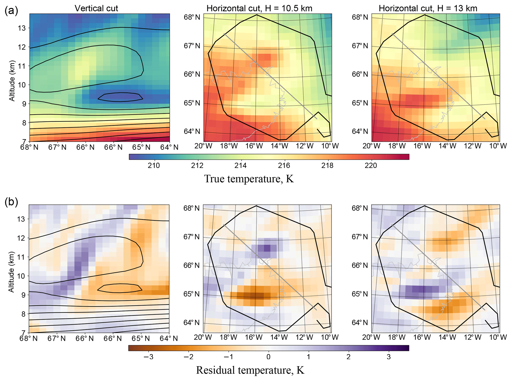
Figure 1 Panel (a) shows the ECMWF temperature data used to generate the synthetic measurements (true temperature). Panel (b) shows the temperature residual: the difference between the true temperature and the smoothed temperature field used as an a priori. In the first column, black lines represent the contours of a priori temperature values. In columns 2 and 3, the black line is the flight path, the thick grey line is the position of the cut shown in the first column and the thin grey line is the topography (Icelandic coastline visible).

4.2 Retrieval set-up and test data

A hexagonal flight pattern intended for tomography was realised on 25 January 2016, as part of flight 10 of the POLSTRACC measurement campaign. The flight path of the HALO research aircraft contained a regular hexagon with a diameter (distance between the opposite vertices) of around 500 km over Iceland, which allowed for a high spatial resolution retrieval in the central part of the aforementioned hexagon (Fig. 1). The flight altitude throughout the hexagonal flight segment remained close to 14 km. For detailed information about this flight refer to Krisch et al. (2017).

The test case used in this paper is based on the actual aircraft path, measurement locations, spectral lines used for retrieval and meteorological situation during this flight. Synthetic measurement data were used instead of real GLORIA observations: the forward model of JURASSIC2 was employed to simulate the observed radiances in the atmospheric state given by the ECWMF temperature and WACCM model data for trace gases. Simulated instrument noise was subsequently added to those radiances. This set-up allows us to use the model data as a reference (the “true” atmospheric state) for evaluation of retrieval quality. The same set of simulated measurements was used for all test retrievals described in this paper. These measurements were obtained by running the forward model on a very dense grid (about twice as dense in each dimension as those of the densest test retrievals). This was done to ensure that the discretisation errors in the simulated measurements would be minimal and would not favour any retrieval (as could happen if they were generated on the same grid). An evaluation of forward model errors on different grids is presented in Appendix C.

The retrieval derives temperature and volume mixing ratios of O₃, HNO₃, CCl₄ and ClONO₂. Temperature and CCl₄ concentration are derived in the altitude range from 3 to 20 km; O₃, HNO₃ and ClONO₂ are retrieved from 3 to 64 km. The latter three trace gases have larger volume mixing ratios above flight level and hence significant contributions to measured radiances from these high altitudes. Interpolated WACCM data were used as an a priori for all trace gases. A priori data for temperature were obtained by applying polynomial smoothing to ECMWF data. The retrieval is hence not supplied with the full temperature structure that was used to simulate the measurement. Therefore, the agreement between the retrieval result and the “true” atmospheric state, upon which the simulated measurements are based, cannot be achieved by overregularisation.

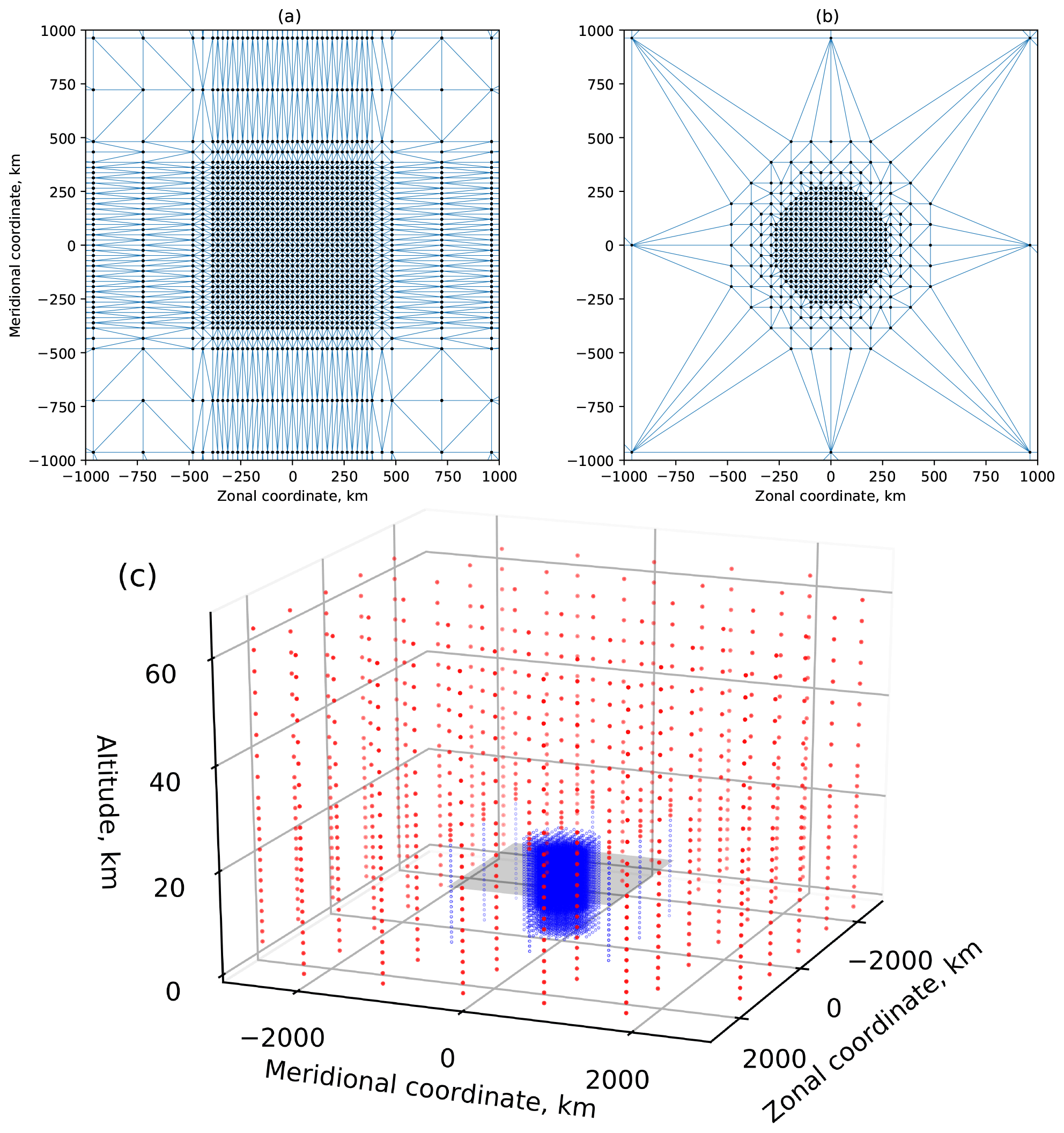
Figure 2 Panels (a) and (b): horizontal cuts of retrieval grids. Dots show grid points; blue lines indicate Delaunay cell boundaries. Panel (a) shows the full initial grid for retrievals A, B and C (all horizontal layers of this grid are identical), (b) shows the thinned-out grid for retrieval D (cut at 11 km). Panel (c) is the grid for retrieval D. Radial distance is defined as distance to the vertical line at the centre of the hexagonal flight path (66^∘ N, 15^∘ W). Points within the inner core (1000 km ×1000 km ×20 km) are shown in blue, other points are in red, and the shaded rectangle shows the position of the horizontal cut in panel (b).

4.3 Correlation length estimation

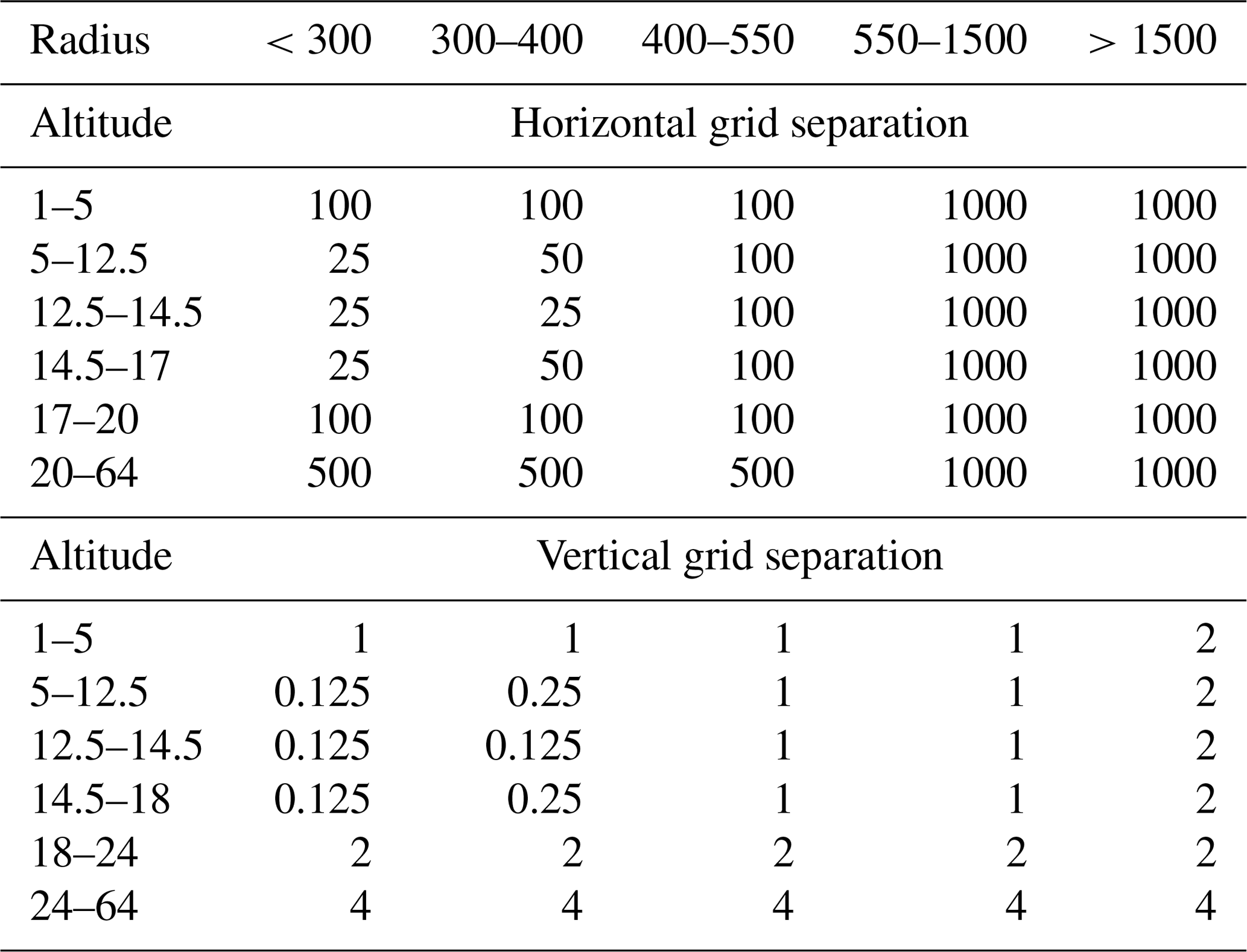
Table 1 Retrieval parameters.

Regularisation weights α₀, α_h, (as in Eq. 2) are used for retrieval A, the standard deviation σ (see Eq. 15) used for retrievals B-D.

The standard deviation σ and correlation of the lengths L_h and L_v in Eq. (13) can be obtained from statistical analysis of in situ measurement or model data. Rigorous derivation of these parameters for each retrieved trace gas and temperature would require detailed analysis of in situ measurement databases and is, therefore, out of scope of this paper. However, the following rough approximation proved sufficient to improve the retrieval results compared to the old regularisation scheme.

3-D tomographic retrievals are most useful for those trace gases that have high vertical gradients and complex spatial structure. The spatial correlation lengths of concentrations of such gases are mostly determined by stirring, mixing and other dynamical processes and are therefore similar. Furthermore, Haynes and Anglade (1997) and Charney (1971) estimated the dynamically determined aspect ratio to be α≈200–250 in the lower stratosphere, and we expect less than that in the upper troposphere. Hence, we will assume $L_{\mathrm{h}}/L_{\mathrm{v}}=\mathrm{200}$ for all trace gases.

An analysis of spatial variability of some airborne in situ measurements was performed by Sparling et al. (2006). For ozone concentration χ(s ,z), where s is the horizontal location and z is the altitude, they define fractional difference parameters:

$$\begin{array}{}\text{(31)}& {\displaystyle }& {\displaystyle }{\mathrm{\Delta }}_{r,h}={\displaystyle \frac{\mathrm{2}\left|\mathit{\chi }\left(s+r,z+h\right)-\mathit{\chi }\left(s,z\right)\right|}{\left[\mathit{\chi }\left(s+r,z+h\right)+\mathit{\chi }\left(s,z\right)\right]}}\text{(32)}& {\displaystyle }& {\displaystyle }{\mathrm{\Delta }}_r=\underset{h\to \mathrm{0}}{lim}{\mathrm{\Delta }}_{r,h}\end{array}$$

and provide the dependence of the standard deviation σ(Δ_r) on the horizontal separation r. If the typical spatial variation in ozone concentration is significantly smaller than the mean ozone concentration 〈χ〉, one can approximate ${\mathrm{\Delta }}_r\approx \left|\mathit{\chi }\left(s+r\right)-\mathit{\chi }\left(s\right)\right|/\langle \mathit{\chi }\rangle$. Then, using the covariance relation (8) and various properties of the normal distribution, we get ${\mathit{\sigma }}^{\mathrm{2}}\left({\mathrm{\Delta }}_r\right)=\mathrm{2}{\left(\mathit{\sigma }/\langle \mathit{\chi }\rangle \right)}^{\mathrm{2}}\left(\mathrm{1}-\mathrm{2}/\mathit{\pi }\right)\left(\mathrm{1}-\exp \left(-r/L_{\mathrm{h}}\right)\right)$. By comparing this to the experimental results of Sparling et al. (2006), we estimate L_h=200 km. Using the aspect ratio argument above, we also set L_v=1 km.

The spatial structure of retrieved temperature differs from that of the trace gases. It is determined not only by mixing and stirring, but also radiative processes and gravity waves. Radiative transfer tends to erase some of the fine vertical structure determined by isentropic transport; hence one should use a greater vertical correlation length than in the case of trace gases. Gravity waves have a variety of length scales, but due to the finite resolution of the instrument not all of them can be retrieved. Following the gravity wave observational filter study for the GLORIA instrument in Krisch et al. (2018) we can estimate the lowest observable gravity wave horizontal wavelength to be λ_h∼200 km and the lowest vertical wavelength to be λ_v∼3 km. λ_h coincides with the dynamically determined correlation length L_h=200 km, so this value should be appropriate for temperature as well. The λ_v limit is not only determined by instrument resolution, but is also related to the fundamental properties of gravity waves. Preusse et al. (2008) gives the following expression for the gravity wave saturation amplitude

$$\begin{array}{}\text{(33)}& {\widehat{T}}_{\max }={\displaystyle \frac{{\mathit{\lambda }}_{\mathrm{v}}\overline{T}{N}^{\mathrm{2}}}{\mathrm{2}\mathit{\pi }g}},\end{array}$$

where $\overline{T}$ is the mean temperature and N is the Brunt–Väisälä frequency. In typical lower stratosphere conditions and when λ_v=3 km, Eq. (33) gives ${\widehat{T}}_{\max }\approx \mathrm{4}\mathrm{K}$. Since gravity waves are usually not saturated and considering typical measurement errors (see Sect. 4.6), waves of significantly shorter wavelengths would probably not be observed. We hence set L_v=3 km. Time series of measurements at a fixed point in the atmosphere are then used to approximate the standard deviations σ for all retrieved quantities (Table 1). Our choice of σ value for temperature, in particular, may seem rather low. This is related to the choice of a priori: smoothed ECMWF data were used instead of climatologies that would have been more typical in this case. Such an a priori can be expected to match the large-scale structures of real temperature more closely, thus reducing the forward model errors in poorly resolved areas and improving the results. It is particularly useful for resolving fine structures, such as gravity waves, which were the main scientific interest of the measurement flight used as a basis for test retrievals (Krisch et al., 2017). A likely closer match between the a priori and retrieval thus requires a lower σ value, that, in this set-up, represents expected strength of gravity wave disturbances, rather than the full thermal variability of the atmospheric region in question.

Table 2 Grid densities in different regions for retrieval D in kilometres.

4.4 Test retrievals

The test data described in the previous section were processed with several different regularisation set-ups and retrieval grids. Here we present the results for four different runs.

Firstly, as a reference, the latest version of JURRASIC2 without the implementation of any new algorithms described in this paper was used (retrieval A). It uses a rectangular grid that covers altitudes from 1 to 64 km. The vertical spacing of the grid is 1 km between the altitudes of 1 and 5 km, 125 m between altitudes of 5 and 20, 1 km between altitudes of 20 and 25 and 4 between 28 and 64 km. As required for the rectilinear grid, the number and distribution of points is the same in each altitude (Fig. 2a). For this reference run, a first-order regularisation (Eq. 1) with trilinear interpolation (Bai and Wang, 2010) was used. The regularisation weights, as defined in Eq. (2), are given in Table 1. These are typically tuned ad-hoc, i.e. adjusted by trial and error until optimal retrieval results can be achieved, starting from the default values obtained as in Hansen and O'Leary (1993). While tuning, the retrieval results are validated against the atmospheric state used to generate the synthetic measurements. When using real observations, the results are validated against in situ measurements and model data.

Figure 3 Panels show the difference between retrieved temperature and true temperature of the simulated atmosphere. Rows A–D show the results of the respective retrievals. In the first column, black lines represent the contours of the a priori temperature value. In columns 2 and 3, the black line is the flight path, the thick grey line is the position of the cut shown in the first column and the thin grey line is the topography (Icelandic coastline visible).

Then, to evaluate the performance of second-order regularisation, retrieval B was performed. The grid and interpolation methods were identical to retrieval A, but the regularisation was replaced with the second-order scheme from Eqs. (13) and (15) and correlation lengths derived in Sect. 4.3 from in situ observations. No subsequent tuning of these parameters was performed.

We compare the quality of different retrievals by inspecting the differences between the retrieved temperature and temperature used to generate the synthetic measurements (“true” temperature). These differences are shown on horizontal and vertical slices of the observed atmospheric volume in Fig. 3. Figure 4 shows the variation of the retrieved and true temperatures on horizontal lines in order to visualise the response of retrievals to different spatial structures in true temperature.

Figure 4 Retrieved temperature at different altitudes in the vertical cut shown in Figs. 1 and 3. Line T represents the true temperature of the simulated atmosphere, A–D are the respective retrievals.

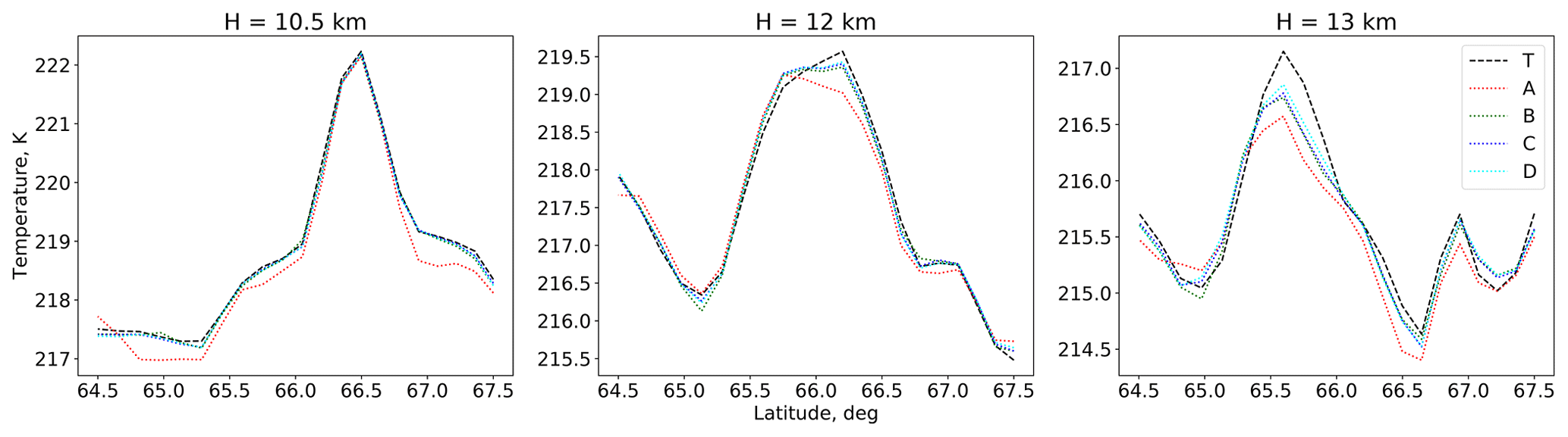
A comparison of Fig. 3A and B shows the effect of the new regularisation (Eq. 13). The new algorithm (retrieval B) demonstrates better agreement with the true temperature. It shows markedly less retrieval noise in the central area, as well as better results (less effect of a priori) just outside it, at the edges of the vertical cut shown in Fig. 3. Considering also that, unlike A, the regularisation strength of B was not manually tuned for this test case in particular, we can conclude that the new regularisation performed better in this test case.

The third retrieval (C) was performed on the same set of grid points as B and with the same input parameters, but the grid was treated as irregular; i.e. a Delaunay triangulation was found. The algorithms described in Sect. 2 were used for regularisation. A horizontal cut of the Delaunay triangulation for this grid is shown in Fig. 2a. By comparing B and C one can evaluate the agreement between the old interpolation, derivative calculation and volume integration techniques for rectilinear grids and their newly developed irregular-grid-capable alternatives. The temperature fields from retrievals B and C are very similar (Fig. 3), which confirms that the new Delaunay-triangulation-based code gives consistent results when run on a rectilinear grid.

Finally, retrieval D was performed with the same input parameters and methods as C, but using only the subset (22 %) of the original grid points to reduce computational cost. These points were chosen so that grid density would be highest in the volumes best resolved by GLORIA and sparser where little measurement data are available. In particular, a set of axially symmetric regions around the centre of original retrieval (i.e. symmetric with respect to vertical axis at 66^∘ N, 15^∘ W) was defined as shown in Table 2. Points were removed from the original grid to achieve the specified vertical and horizontal resolutions for each region, resulting in the grid shown in Fig. 2. Results changed little compared to retrieval C. Most of the minor differences between C and D occur near the edges of the hexagonal flight path (Fig. 3). Even though the grid spacing for retrieval D is still the same as C in some these areas, larger grid cells nearby have some effect on their neighbours. Note also that C and D retrievals tend to differ in the areas where the agreement between each of them and the true temperature is relatively poor and diagnostics predict lower accuracy (Fig. 5), so D can be considered to be as good as C in well-resolved areas. Unphysical temperature structures far outside the measured area, like the one partially seen at 64^∘ N, 20^∘ W, are not unique to this retrieval. They just occur a little closer to the flight path in this case due to the coarser grid outside the hexagon.

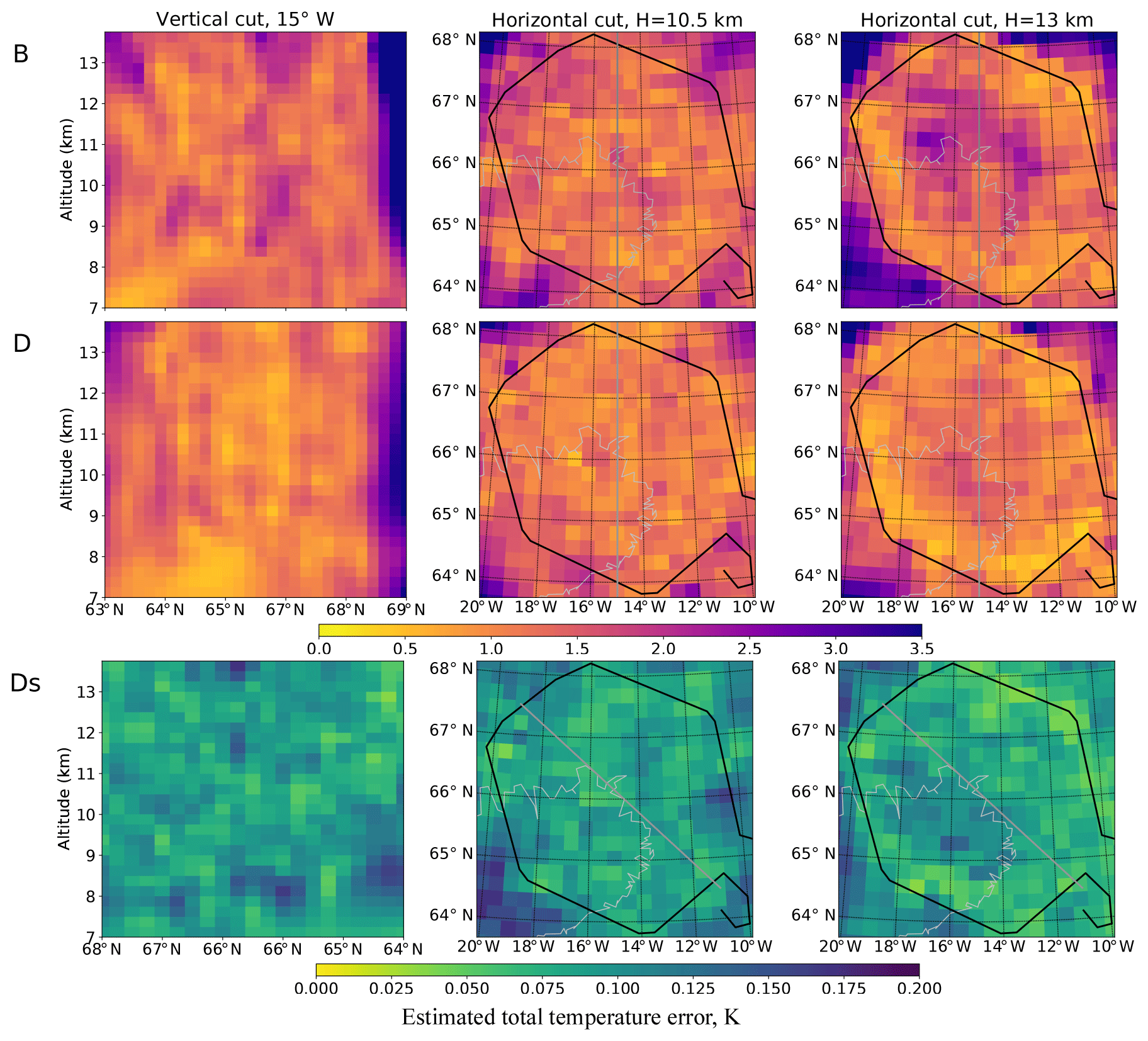
Figure 5 Panels B and D show the Monte Carlo estimate of the total temperature error the retrievals B and D would have if the measurements were real. Panel Ds shows an error estimate for the synthetic retrieval D (this assumes that unretrieved quantities, e.g. pressure, are known exactly). In columns 2 and 3, the black line is the flight path, the thick grey line is the position of the cut shown in the first column and the thin grey line is the topography.

4.5 Computational costs

JURASSIC2 finds an atmospheric state minimising Eq. (1) iteratively. In each iteration it first computes a Jacobian matrix of the forward model and hence obtains a Jacobian of the cost function (1), then minimises the cost function using the Levenberg–Marquardt (Marquardt, 1963) algorithm and by employing conjugate gradients (CG) (Saad, 2003, Hanke, 1995) to solve the linear systems involved. The forward model is then run to simulate the measurements for the new iteration of the atmospheric state.

All calculations were performed on the Jülich Research on Exascale Cluster Architectures (JURECA) supercomputer operated by the Jülich Supercomputing Centre (Jülich Supercomputing Centre, 2016). Each retrieval was executed in parallel on four computational nodes, each with 24 CPU cores (twin Intel Xeon E5-2680 v3 CPUs) and 128 GB of system main memory.

Table 3 shows the time required for different parts of calculation averaged over three identical runs (although <1 % variation was observed). The “other calculations” field mostly includes the time required by input and output, but also preparatory steps such as the Delaunay triangulation in the case of retrievals C and D.

The results in Table 3 reveal the impact of the new methods on computation times. The new, more complex regularisation results in slower convergence in the conjugate gradient calculation, making retrieval B about 6 % more expensive than A. The Delaunay triangulation, however, decreases Jacobian calculation costs by roughly 25 %, even the one used on the same grid as the old approach. This has to do with the fact that interpolation based on Delaunay triangulation only requires four values of the interpolated quantity at neighbouring points, and linear interpolation in three directions requires eight, thus resulting in more non-zero terms in the Jacobian. The time required for the initialisation of the Delaunay interpolation and derivatives, including construction of the matrix ${\mathbf{S}}_{\mathrm{a}}^{-\mathrm{1}}$, increases rather fast with grid size with current implementation, contributing to “other calculations” of retrieval C. Further optimisation of this step is possible and will be implemented in the future. In total, the new retrieval (C) is 9 % faster then the old approach (A) while using the same grid.

Table 3 Computational cost of retrievals (calculation times given in minutes).

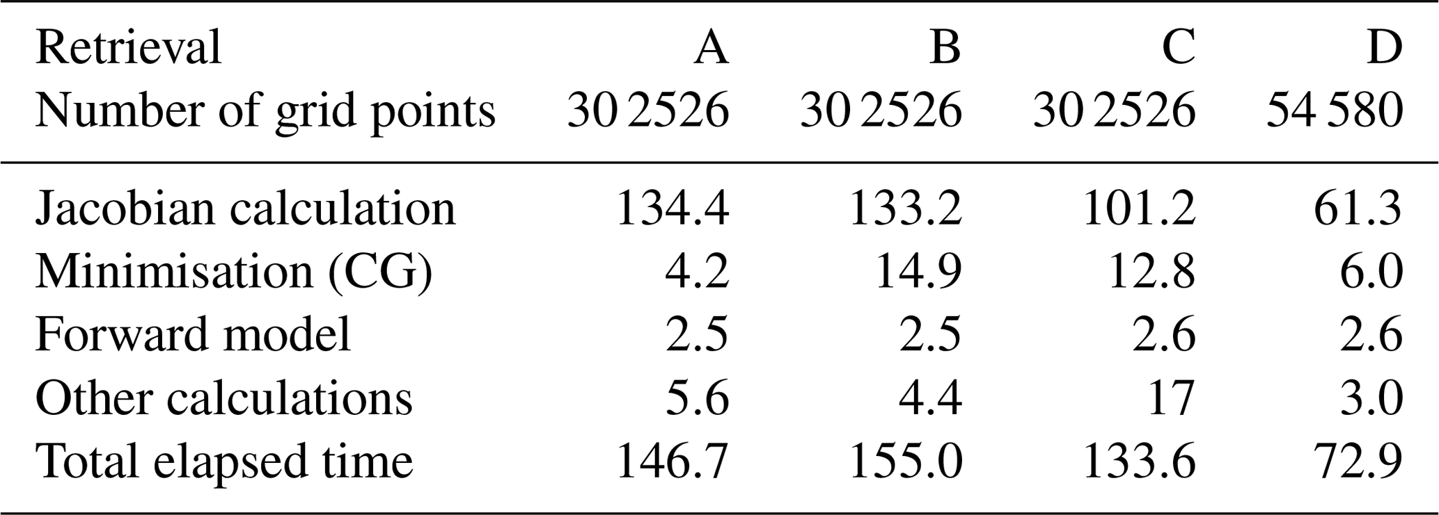
Retrieval D gives a further 45 % reduction of the computation time by removing 82 % of points in the grid. A speed-up of such an order was expected. Only a minority of grid points contribute to a forward model (and hence Jacobian) calculations, and JURASSIC2 code is heavily optimised for sparse matrix operations. Most of the grid points contributing to the forward model are in the areas well resolved by the instrument and thus cannot be removed from the grid without compromising data products. Therefore, the actual savings in computation time mostly come from removing points above a flight level and choosing a more appropriate non-rectangular shape for the densest part of the grid when measurement geometry requires it. Some of the points above the flight path must be included since infrared radiation from there is measured by the instrument, but very little information about atmosphere far above the flight level can be retrieved, so very low grid densities are sufficient (Table 2).

4.6 Diagnostics

We follow Ungermann et al. (2011) and use Monte Carlo approach to obtain diagnostics, but replace Cholesky decomposition with the method developed in Sect. 3. Results for retrievals B and D are presented in Fig. 5B and D. They show the total error estimate for temperature based on the sensitivity of temperature value to (simulated) instrument noise and all other retrieved atmospheric quantities as well as the expected error of non-retrieved quantities (e.g. pressure). These results tell us what temperature errors we could expect if the retrievals in question were performed with real data. Panel Ds shows an error estimate based on (simulated) instrument noise and uncertainties of retrieved parameters only. In the case of a synthetic retrieval, unretrieved parameters, upon which the simulated measurements are based, are known exactly. Therefore, panel Ds is a direct Monte Carlo prediction of the temperature deviation seen in Fig. 3D, and the magnitude of this deviation is indeed similar.

These results confirm that temperature can only be reliably retrieved within the flight hexagon or very close to the actual path. Also, the error estimates are higher in the central area of hexagon, close to flight altitude, in agreement with test results (compare column 3 of Figs. 3 and 5).

Monte Carlo retrieval results provided here were verified by estimating the temperature error at one grid point using a more direct approach. Rodgers (2000) proves that the retrieved atmospheric state x can be written in terms of the a priori state x_a, the (unknown) true state x_t and measurement error ϵ as

$$\begin{array}{}\text{(34)}& \mathit{x}=\mathbf{A}{\mathit{x}}_{\mathrm{t}}+\left(\mathbf{I}-\mathbf{A}\right){\mathit{x}}_{\mathrm{a}}+\mathbf{G}\mathit{ϵ},\end{array}$$

where

$$\begin{array}{ll}{\displaystyle }& {\displaystyle }\mathbf{G}={\mathbf{M}}^{-\mathrm{1}}{\left(\mathbf{DF}\left(\mathit{x}\right)\right)}^T{\mathbf{S}}_{\mathit{ϵ}}^{-\mathrm{1}}\mathbf{A}=\mathbf{G}\mathbf{DF}\left(\mathit{x}\right)\\ \text{(35)}& {\displaystyle }& {\displaystyle }\mathbf{M}={\mathbf{S}}_{\mathrm{a}}^{-\mathrm{1}}+{\left[\mathbf{DF}\left(\mathit{x}\right)\right]}^T{\mathbf{S}}_{\mathit{ϵ}}^{-\mathrm{1}}\mathbf{DF}\left(\mathit{x}\right).\end{array}$$

Here, D denotes the Jacobian operator and all other notation as in Eq. (1). The so-called gain matrix G fully describes the effect of measurement uncertainties ϵ on the retrieved state x. Computing G would be prohibitively expensive due to the required matrix inversion, but note that the i'th element of x only depends on the i'th line of the matrix G, so one can use Krylov subspace methods (e.g. conjugate gradients) to solve Mr_i=e_i for the i'th row ${\mathit{r}}_i^T$ of the inverse matrix M⁻¹. The i'th row of G can then be obtained as ${\mathit{r}}_i^T{\left(\mathbf{DF}\left(\mathit{x}\right)\right)}^T{\mathbf{S}}_{\mathit{ϵ}}^{-\mathrm{1}}$.

This approach allows for error estimation for a small number of grid points in a reasonable amount of time. We chose one point at the centre of the hexagon (66^∘ N, 15^∘ W, 11.75 km altitude) for retrieval B. The total temperature error was found to be 1.27 K and agrees with the Monte Carlo result (1.25 K) at this point within 2 %, which is an excellent accuracy for an error estimate.

5 Conclusions

A new regularisation algorithm for 3-D tomographic limb sounder retrievals employing second spatial derivatives (based on Eqs. 13, 15) was developed and implemented. The ad-hoc parameters (regularisation weights) of the previous first spatial derivative-based approach were replaced with physical quantities – retrieved quantity standard deviation and correlation lengths in vertical and horizontal directions. Unlike the regularisation weights, these quantities do not require manual tuning for each retrieval and can be estimated from in situ measurements, model data and theoretical considerations. Tests with synthetic data showed a slightly superior performance of the new algorithm, even compared to the old approach with tuned parameters. A rather general technique (Eq. 10) of adapting the tomographic retrieval for atmospheric regions of high anisotropy and spatial variability was also proposed.

A Delaunay-triangulation-based approach for retrievals on irregular grids was developed. By better adapting the grid to the retrieval geometry and thinning it out in the regions where a lack of measurement data limits the resolution, the computation time of a tomographic retrieval was reduced by a total of 50 % without significant deterioration of the results. Irregular grids can be further employed for efficient tomographic retrievals in non-standard measurement geometries. At the time of writing, the methods developed in this paper were already in use to process GLORIA limb sounder data.

Monte Carlo diagnostics were newly implemented for a 3-D tomographic retrieval, allowing for quick and reliable evaluation of measurement quality, identification of reliably resolved volumes and selection of optimal 3-D tomography set-ups. Error estimates for retrieved atmospheric quantities can now be calculated at each grid point, while the previous approaches to diagnostics only allowed us to do that for a few selected points within a similar time frame.

Appendix A: Regularisation tests

Equation (15) was used to construct precision matrices ${\mathbf{S}}_{\mathrm{a}}^{-\mathrm{1}}$ directly, since constructing a covariance matrix S_a explicitly and inverting it would be prohibitively computationally expensive. While Eq. (13) was derived analytically, its discrete implementation cannot be exact, which raises the question of whether our precision matrices still have required properties, namely whether they are still inverses of S_a, which obeys Eq. (8). Clearly, this can only be verified directly for a small test case, where covariance matrices are small enough to be inverted. Also, employing matrix norms to compare matrices is not very useful in this case, as the directly computed ${\mathbf{S}}_{\mathrm{a}}^{-\mathrm{1}}$ is based on finite difference derivative estimates which do not work very well at grid boundaries. This is not a problem for the retrieval, which, by design, approaches the a priori state near grid boundaries, but it has strong effects on matrix norms. Instead, we compared the covariance matrices by using them to compute the norms of several test vectors, which represent typical structures expected for that covariance.

Precision matrix ${\mathbf{S}}_{\mathrm{a}}^{-\mathrm{1}}$ was constructed for one entity on a regular $\mathrm{20}\times \mathrm{20}\times \mathrm{20}$ grid (grid constant 1 in each direction) using the same techniques as for retrieval B (σ=1 and $L_{\mathrm{v}}=L_{\mathrm{h}}=L=\mathrm{2}$). Then a covariance matrix was explicitly constructed for the same grid using Eq. (8) and inverted to obtain the precision matrix ${\widehat{\mathbf{S}}}_{\mathrm{a}}^{-\mathrm{1}}$. A set of vectors x_ϕ was computed – discrete representations of a “Gaussian wave packet” disturbance

$$\begin{array}{}\text{(A1)}& \mathit{\varphi }\left(\mathit{r}\right)=\exp \left(-{\displaystyle \frac{\Vert r{\Vert }^{\mathrm{2}}}{d^{\mathrm{2}}}}\right)\cos \left(\mathit{k}\cdot \mathit{r}\right).\end{array}$$

The parameter d was chosen so that the amplitude of the wave would decay to at most 0.01 at the grid boundary, thus suppressing edge effects. Two different wavelengths, namely $\mathit{\lambda }=\mathrm{15},\mathrm{20}$, in grid units, were chosen, and 50 k values pointing in every possible direction were generated for each wavelength (i.e. $\Vert \mathit{k}\Vert =\mathrm{2}\mathit{\pi }/\mathit{\lambda }$). Then, for each of the resulting 100 disturbances, the norms $\Vert {\mathit{x}}_{\mathit{\varphi }}{\Vert }_p$ and $\Vert {\mathit{x}}_{\mathit{\varphi }}{\Vert }_{\mathrm{t}}$, where $\Vert {\mathit{x}}_{\mathit{\varphi }}{\Vert }_p^{\mathrm{2}}={\mathit{x}}_{\mathit{\varphi }}^T{\mathbf{S}}_{\mathrm{a}}^{-\mathrm{1}}{\mathit{x}}_{\mathit{\varphi }}$ and $\Vert {\mathit{x}}_{\mathit{\varphi }}{\Vert }_{\mathrm{t}}^{\mathrm{2}}={\mathit{x}}_{\mathit{\varphi }}^T{\widehat{\mathbf{S}}}_{\mathrm{a}}^{-\mathrm{1}}{\mathit{x}}_{\mathit{\varphi }}$, were calculated, as well as their relative difference $\mathit{\delta }=\mathrm{2}\left|\Vert {\mathit{x}}_{\mathit{\varphi }}{\Vert }_p-\Vert {\mathit{x}}_{\mathit{\varphi }}{\Vert }_{\mathrm{t}}\right|/\left(\Vert {\mathit{x}}_{\mathit{\varphi }}{\Vert }_p+\Vert {\mathit{x}}_{\mathit{\varphi }}{\Vert }_{\mathrm{t}}\right)$. For the case λ=15 we found that the mean δ value was 0.050, with a standard deviation of 0.0042, and for the case λ=20 the mean was 0.036, with a standard deviation of 0.0007. We believe that a precision of this order is sufficient for regularisation purposes.

Table A1 Forward model tests.

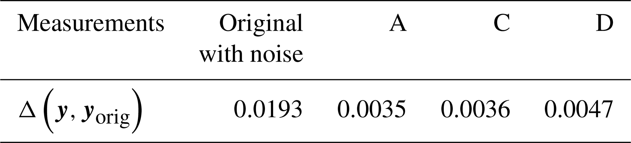
Difference in forward model results compared to original synthetic measurement set without noise. A–D refer to the forward model results of respective retrievals.

Appendix B: Applicability to 1-D and 2-D retrievals

The exponential covariance relation given in Eq. (8) can be trivially extended to any dimension. It is used as a statistical model to many processes. The norm associated with this exponential covariance given in Eq. (9) is, however, a 3-D-specific result. Known 2-D equivalents involve fractional powers of derivatives and therefore are not as easy to implement numerically. A norm associated with 1-D exponential covariance can be shown (Tarantola, 2013) to have the simple form

$$\begin{array}{}\text{(B1)}& \Vert \mathit{\varphi }{\Vert }^{\mathrm{2}}={\displaystyle \frac{\mathrm{1}}{\mathrm{2}{\mathit{\sigma }}^{\mathrm{2}}L}}\left(\underset{x_{\mathrm{1}}}{\overset{x_{\mathrm{2}}}{\int }}{\mathit{\varphi }}^{\mathrm{2}}\mathrm{d}x+L^{\mathrm{2}}\underset{x_{\mathrm{1}}}{\overset{x_{\mathrm{2}}}{\int }}{\left({\displaystyle \frac{\partial \mathit{\varphi }}{\partial x}}\right)}^{\mathrm{2}}\mathrm{d}x\right),\end{array}$$

neglecting some boundary terms. Here the scalar field ϕ(x) represents the difference between the quantity to be retrieved and the a priori, and L is the correlation length. All the main theoretical results and numerical methods of this paper can therefore be reproduced for 1-D inverse modelling problems. The usefulness of our methods for practical 1-D applications ultimately depends on the size of the problem in question. 1-D limb sounding retrievals, for example, are usually too small for the methods developed here to be useful. It would typically be possible, and indeed simpler, to explicitly construct and invert the covariance matrix of a 1-D problem, rather than discretise the associated norm (Eq. B1). In the case of a very large 1-D problem with a strong covariance, however, one may find the methods presented in this paper to be more lucrative.

Appendix C: Forward model tests

As pointed out in Sect. 4.2, the same measurement set, synthetically generated on a dense grid, was used for retrievals A–D. This provides an easy way to verify whether the forward model is performing consistently on different grids: run it on each grid based on the ”true” atmospheric state and compare the results with the synthetic measurements from the dense grid. In our test case, the radiances are calculated for n=31 spectral windows. If vector y represents a set of radiances, and y_i represents the radiances at ith spectral window, we evaluate the difference between those vectors with the parameter $\mathrm{\Delta }\left(\mathit{y},{\mathit{y}}^{\mathbf{\prime }}\right)=(\mathrm{1}/n){\sum }_i^n\mathrm{2}\Vert {\mathit{y}}_i-{{\mathit{y}}^{\mathbf{\prime }}}_i{\Vert }_{\mathrm{2}}/(\Vert {\mathit{y}}_i{\Vert }_{\mathrm{2}}+\Vert {{\mathit{y}}^{\mathbf{\prime }}}_i{\Vert }_{\mathrm{2}})$, where $\Vert \cdot {\Vert }_{\mathrm{2}}$ is the euclidean norm. The results of this comparison are presented in Table A1. The forward model for retrievals A and C used the same grid, but A used trilinear interpolation, and C used Delaunay interpolation. We can see that the change in interpolation does not introduce significant errors (compared to those introduced by the grid change). Thinned-out grid and Delaunay interpolation was used for grid D. Note that the simulated measurements that were actually used also have simulated instrument noise added to them. The results clearly show that the effects of different discretisation are well below the instrument noise level. Also, the error is lower than our generally assumed forward model error of 1 %–3 % (Hoffmann, 2006).