the Creative Commons Attribution 4.0 License.
the Creative Commons Attribution 4.0 License.
 | 19 Mar 2020
Calibration and validation of the Polarimetric Radio Occultation and Heavy Precipitation experiment aboard the PAZ satellite
Chi O. Ao
F. Joseph Turk
Manuel de la Torre Juárez
Byron Iijima
Kuo Nung Wang
Estel Cardellach
This paper presents the calibration and validation studies for the Radio Occultation and Heavy Precipitation experiment aboard the PAZ satellite. These studies, necessary to assess and characterize the noise level and robustness of the differential phase shift (ΔΦ) observable of polarimetric radio occultations (PROs), confirm the good performance of the experiment and the capability of this technique in sensing precipitation. It is shown how all the predicted effects that could have an impact into the PRO observables (e.g., effect of metallic structures nearby the antenna, the Faraday rotation at the ionosphere, signal impurities in the transmission, and altered cross-polarization isolation) are effectively calibrated and corrected, and they have a negligible effect on the final observable. The on-orbit calibration, performed using an extensive dataset of free-of-rain and low-ionospheric activity observations, is successfully used to correct all the collected observations, which are further validated against independent precipitation observations confirming the sensitivity of the observables to the presence of hydrometeors. The validation results also show how vertically averaged ΔΦ can be used as a proxy for precipitation.
- Article
(7518 KB) - Full-text XML
- BibTeX
- EndNote


The Radio Occultation and Heavy Precipitation (ROHP) experiment on board the PAZ satellite was switched on on 10 May 2018, after a successful launch on 22 February 2018. For the first time, radio occultations (ROs) are acquired at two linear polarizations with the aim to detect heavy precipitation. The technique, called polarimetric RO (PRO), consists of measuring the phase difference between the horizontal (H) and vertical (V) components of the electromagnetic field coming from the global positioning system (GPS) satellites in occulting geometry (Cardellach et al., 2014). This is an augmentation of the capabilities of the well-known RO technique (e.g., Kursinski et al., 1997; Hajj et al., 2002). The first preliminary results obtained during the first 5 months of data confirm that the measurement is sensitive to precipitation (Cardellach et al., 2019).
H and V components are measured independently, yet synchronously, with a dual linearly polarized antenna pointing towards the limb of the Earth in the anti-velocity direction of the satellite. The rays, curved and delayed as they penetrate into deeper layers of the atmosphere (with higher density), reach the receiver in occultation geometry. The delay of the rays can be precisely tracked, and information about the thermodynamic state of the atmosphere can be retrieved (e.g., vertical profiles of temperature, pressure, and water vapor pressure) as in standard RO. The fact that in the PAZ satellite the incoming electromagnetic field is acquired at two linear and orthogonal polarizations allows us to retrieve information about media that introduce a differential phase shift between the horizontal and vertical components of the propagating electromagnetic waves. The media introducing this effect are mainly hydrometeors that flatten due to air drag as they fall. The scattering of electromagnetic waves by these asymmetric hydrometeors introduces a differential change in phase between the H and V components that is proportional to the amount and size of the hydrometeors. Therefore, this experiment represents the first technique able to retrieve vertical information about precipitation and the thermodynamic state of the surrounding area within the same measurement, from space.
The first analysis (Cardellach et al., 2019) was focused only on the ability of the technique to detect hydrometeors, and a thorough calibration of the receiving system is required before more quantitative results can be obtained. The calibration of the receiving system is critical in assessing the uncertainty level of the measurement and therefore to associate geophysical quantities like rain intensity to each phase measurement (Cardellach et al., 2018). This would enable a wide range of studies and concepts taking full advantage of PRO capabilities, such as those proposed in Padullés et al. (2018), Turk et al. (2019), and Murphy et al. (2019).
The purpose of the calibration of the receiving system is to remove the systematic effects unrelated to hydrometeors (Tomás et al., 2018). These include the ionospheric effect on the polarimetric signal, the impurity of the transmitted signal, the ambiguity introduced by the receiver tracking two independent signals, and any other instrumental effects. In addition, the environment around the receiving antenna needs to be characterized. Before launch, a metallic structure had to be added to the satellite in order to adapt it to the a new launch vehicle (see Fig. 1a). This structure sits 30 mm above the antenna and covers part of the field of view. It introduces a systematic effect that depends on the angle of arrival of the signal at the antenna and changes the antenna patterns from those measured in an anechoic chamber before installation (Cardellach et al., 2014). It is also very likely that the metallic structure has worsened the cross-polarization isolation of the antenna.
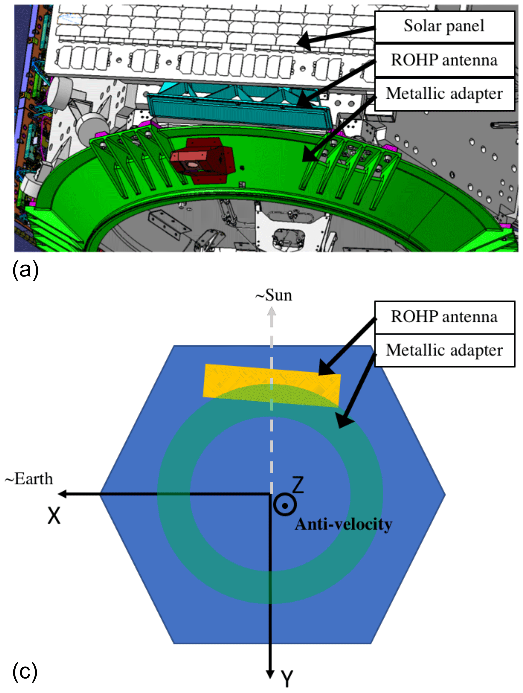
Figure 1(a) Schematic drawing of the metallic adapter structure (green) over the ROHP antenna (blue) and their position in the satellite. Image provided by Hisdesat. (b) Sketch of the satellite body (blue), ROHP antenna (yellow), and the metallic adapter (green) and the body-fixed Cartesian reference frame with the x axis (X) pointing toward the direction of the Earth, the z axis (Z) pointing towards the anti-velocity direction, and the y axis (Y) being the third orthogonal component to define the reference frame.
In order to calibrate the signal, all the available data from 10 May 2018 to 10 October 2019 are accumulated and grouped based on the corresponding precipitation information: the data are classified into clear skies and cloudy–rainy scenes. This classification is performed using information from the National Centers for Environmental Prediction Climate Prediction Center (NCEP CPC) infrared brightness temperature (Janowiak et al., 2017) and Integrated Multi-satellitE Retrievals for the Global Precipitation Measurement (GPM) mission (IMERG) (Huffman et al., 2019) rain rates. This allows us to determine the uncertainty in the measurement when no hydrometeors are present so that there is nothing expected to introduce changes in the differential phase between H and V. Then, the effect of the ionosphere (through Faraday rotation) is assessed using colocations between the simulated RO ray paths and the International Geomagnetic Reference Field (IGRF) Earth's magnetic field model (Thébault et al., 2015) and the International Reference Ionosphere (IRI) climatology for the electron density (Bilitza et al., 2017). Finally, the uncertainty and biases introduced by the antenna are characterized so that they can be corrected in each measurement.
Once the receiving system has been calibrated and the data accordingly corrected, these new observables are validated using the GPM products mentioned above. The results of the validation are compared with what was obtained in Cardellach et al. (2019) and also with the predicted performance from the simulations in Cardellach et al. (2014).
The data collected by the PAZ satellite are downlinked by Hisdesat. The Institut de Ciències de l'Espai (ICE), Consejo Superior de Investigaciones Científicas, Institut d'Estudis Espacials de Catalunya (CSIC, IEEC) collects and owns the data and provides access to the servers at the Jet Propulsion Laboratory (JPL). At the JPL, the raw data are processed and converted to level 1 RO products, which are finally analyzed.
2.1 Polarimetric phase calibration
The JPL-designed Integrated GPS Occultation Receiver (IGOR+) installed in PAZ collects RO data at a rate of 50 Hz. In the PAZ configuration, only setting occultations are tracked. The receiver uses both closed-loop (CL) and open-loop (OL) tracking modes, depending on the altitude (transition from CL to OL happens around 7–9 km). Each RO is tracked independently in the two ports dedicated to the H and V polarized antennae. Therefore, each port output is processed independently. Raw phase data can be converted into excess phase (ϕ) using precise orbit determination (POD); the excess phase identifies the phase delay of the incoming electromagnetic field after removing the geometric contribution (i.e., the distance between satellites and their relative movement) (Hajj et al., 2002). Errors due to satellite and receiver clocks are also corrected. Hence, ϕ is due to atmospheric effects. Its variation as a function of time, i.e., Doppler shift, is the main observable for ROs.
The signal amplitude, or signal-to-noise ratio (SNR), and ϕ(t) from each antenna port are used to obtain the bending angle as a function of the impact parameter, α(a), using the canonical transform method (Gorbunov, 2002). Then, under the assumption of an spherical symmetric atmosphere, the inverse Abel transform (Fjeldbo et al., 1971) is used to retrieve the profile of refractivity as a function of geometric height, N(h). This process is the same one applied to in conventional GNSS RO, and it can also be applied in this case.
The main new observable for PRO, the difference between ϕ(t) of both ports, is
ΔΦ(t) should be constant in time if nothing along the ray path is introducing a differential phase shift. Notice that the absolute phase difference between the H and V components of a righthanded circularly polarized (RHCP) electromagnetic wave should be π∕2; however, since the two components are tracked independently and what remains is the excess phase, this difference is no longer π∕2 but a constant random number. When precipitation is present in any point along the ray path, ΔΦ(t) should increase.
Even though the initial processing of the raw data corrects for cycle slips (i.e., changes in ϕ of more than one cycle in consecutive measurements), after computing ΔΦ(t) some jumps in the observable are detected. These jumps are associated with cycle slips that remained uncorrected before, and after computing the difference between the two ϕ(t) (H and V) became more evident. During CL tracking that occurred above ∼7–9 km altitude, the phase is obtained with half-cycle ambiguity (Ao et al., 2003). During OL tracking that occurred below ∼7–9 km altitude, the tracking data are processed on the ground with the 50 Hz navigation modulation removed, which enables full-cycle phase reconstruction (Ao et al., 2009; Sokolovskiy et al., 2006). Therefore, we correct for half-cycle slips during CL and full-cycle slips during OL, as follows: for the CL region, we apply
and for the OL region we apply
This approach corrects the half and full cycle slips remaining in the data. An example of the remaining cycle slips and their correction can be seen in Fig. 2.
For each port, data are processed to obtain N(h). To assign a height to each time measurement (e.g., excess phase or SNR) is complicated, especially when atmospheric multipath is present at the lower layers. To do so we proceed as follows: using geometric optics (GO) retrievals (e.g., Hajj et al., 2002), we obtain an approximated relationship between the impact parameter and received time, aGO(t). This is then used to map the canonically transformed impact parameter aCT to a unique time t. We then rely on the inverse Abel transform, and we assign a tangent height (the height of the tangent point of each ray) to each phase and SNR measurement, ΔΦ(ht) and SNR(ht). As we said, this is not exact since the relation aGO(t) contains errors under atmospheric multipath conditions. We have estimated (not shown here) that the uncertainty due to atmospheric multipath varies from 0.1 km at 6 km altitude to 0.6 km at 2 km altitude in the tropics, improving at higher latitudes. Therefore, measurements linked to altitudes lower than 2 km have to be treated with caution.
As a convention, the height that is assigned to each time is the mean of the heights obtained in the H and V ports at that time. To set a common reference for all the data that is independent on the initial phase of the receiver, we set the zero at 30 km, and therefore . At this height we know that there is no rain, clouds, or ice that could infer any measurable differential phase shift. Therefore, all measurements are relative to that height.
The whole processing is applied to 96 446 occultations collected between 10 May 2018 and 10 October 2019, of which a total of 74 604 pass through the JPL quality control. The quality control is passed if the retrieved refractivity profiles between 0 and 30 km (for both H and V) are within 10 % of the colocated NCEP Global Forecast System (GFS). Those that do not pass the quality control are discarded.
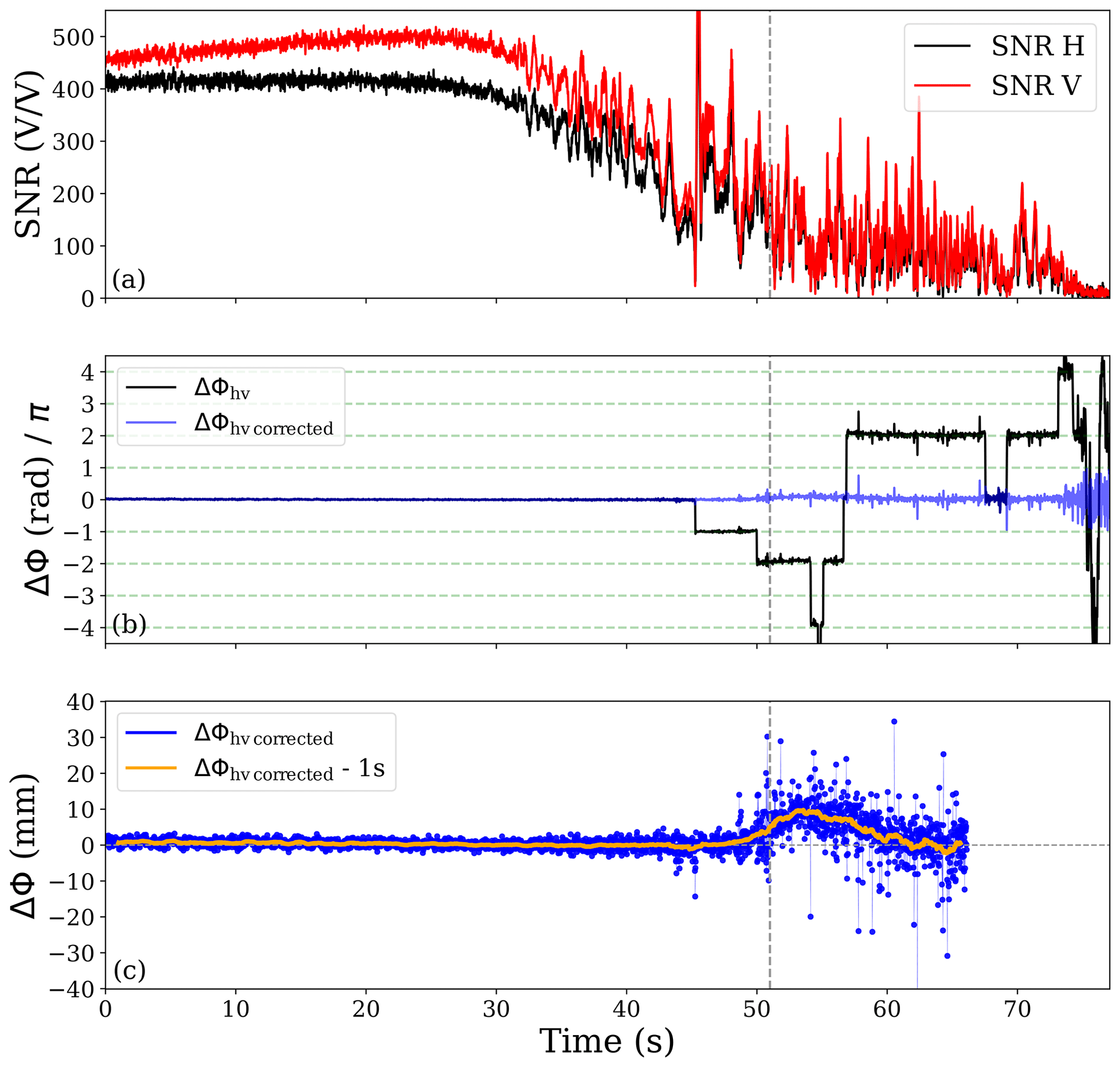
Figure 2Example of one polarimetric RO observation, corresponding to ID 20180827_2108paz_gps57. The RO tangent point is located at 46.5∘ N, 165.3∘ E. (a) SNR for H (black) and V (red) ports as a function of time. (b) Raw differential phase shift between the H and V excess phase observables (black) and the same observable after being corrected for cycle slips, following the procedure in Sect. 2.1. Notice that before the CL to OL transition (gray vertical line), there are two half-cycle slips (jumps of π), while after the transition, several full-cycle slips (jumps of 2π) appear. (c) Corrected differential phase shift (blue) and the corresponding 1 s smoothed measurement (simple average running window). In the bottom part, the differential phase shift is truncated where the corresponding retrieval stops.
2.2 Ray tracing
In order to identify the region that is being sensed by the PRO, we need to define the RO plane. The RO plane is formed by all the rays from the GPS transmitter to the receiver. This plane is slant rather than vertical due to the relative movement between the GPS and the low Earth orbit (LEO) satellite which are not coplanar. To define a realistic RO observation plane, we account for realistic rays between the GPS and the LEO obtained using a ray-tracing software that provides the trajectories of the ray for every time step of the PRO event. The ray tracing uses the retrieved refractivity profile to account for the bending of the rays.
The whole set of trajectories, e.g., time, long, lat, and height, can be used to identify the regions traversed by the rays and therefore perform realistic and accurate colocations between different datasets (like precipitation) for reliable calibration and validation of the experiment.
2.3 Colocation of PRO observations with GPM constellation products
For the calibration and validation part of the experiment, the colocation with precipitation products is crucial. It provides an independent measure on whether an observation might have been affected by rain or not. Since the effect of rain is the objective and it should exhibit a clear distinct signature from the no rain events, the calibration of the receiving system should be done with the rain-free events. Therefore, colocation with precipitation products has to be as accurate as possible.
We consider that the IMERG precipitation products are the best suited for such colocation. First of all, these products provide information about precipitation, covering between ±60∘ in latitude and all longitudes with a high spatial resolution (i.e., 0.1∘×0.1∘), offering the best global coverage among precipitation products. The 30 min time resolution of IMERG products is also acceptable for the colocations that we need.
For the first analysis of the ROHP-PAZ data (Cardellach et al., 2019), where we aimed for a quick look of the sensitivity of PRO observations to precipitation events, we linked every occultation with the intensity of precipitation in the surrounding areas, using cells of fixed size and circularly shaped (e.g., 2 and 0.6∘ of diameter). Although this approach was effective, here we perform a more accurate colocation using the actual shape and orientation of the PRO-sensed region. The region that is sensed by PRO observations can be approximated by a slant vertical plane (RO observation plane; see Sect. 2.2). This results in a sensed region that is long in the direction parallel to the line between the GPS and the LEO but that also has a certain width in the cross direction when projected to the ground. Since the IMERG precipitation product only provides surface precipitation (2D), the ground projections of the RO observation plane are what we use to define the region in which we average the precipitation intensity. This region, however, is defined using only the portion of the RO observation plane below a certain altitude, since we only expect precipitation to have an effect to the lowest portions of the rays.
In order to use the projection to the ground of the RO observation plane, we need to assume that precipitation has some vertical structure and the rays above the surface level can be affected by precipitation as well. Therefore, we use two different heights to define the maximum height at which the rays might be affected by the precipitation: 6 and 12 km. These two altitude values define the portion of the RO plane that we project on the surface and therefore the area in which we average precipitation. For example, when using the 6 km threshold, the RO plane to be projected on the surface will be defined only by the portions of the rays below 6 km. The higher the altitude, the larger the area will become. An example of the colocation strategy is shown in Fig. 3. Using the strategy described above we can reduce the cases in which the ray does not cross precipitation, but it would be labeled as rainy in a 2∘ circular colocation and reduce the uncertainty in the colocations that might have appeared in Cardellach et al. (2019).
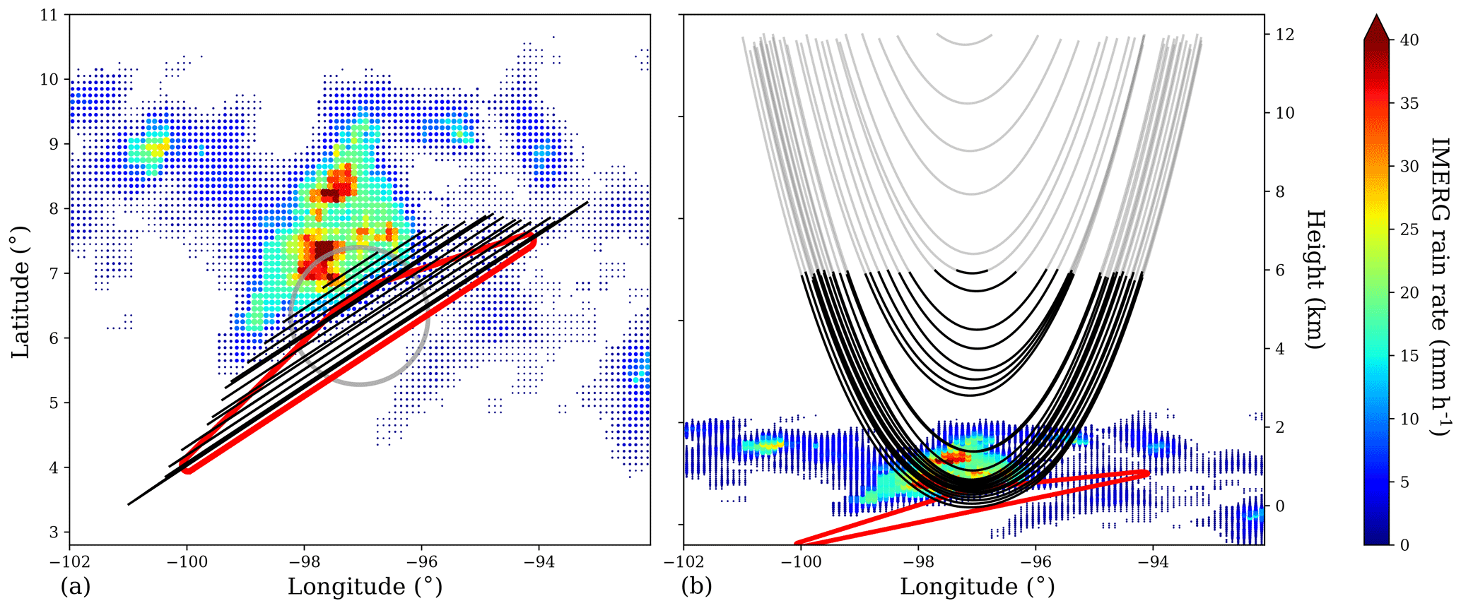
Figure 3Example of the colocation strategy. (a) The black lines show the projection on the surface of the portion of the RO rays below an altitude of 6 km. As the observation descends, longer ray segments reach below the altitude thresholds; therefore the shortest segments represent the higher rays. The red line defines the region where the precipitation is evaluated. For comparison purposes, a circle (gray) of 2∘ of diameter – used in Cardellach et al. (2019) – is shown. The background color is the surface precipitation rain rates from IMERG at a ∘ resolution. (b) The RO rays shown in a longitude–height projection. The darkest part of the rays represent the portion below 6 km. The background IMERG surface precipitation (same as in a) is shown here as a 3D projection, where the x axis corresponds to longitude and the y axis to latitude (all values are contained in the longitude–latitude plane). Only a few RO rays are shown here for illustration purposes.
For the rest of the paper, when we refer to the precipitation associated with a PRO event, we will be referring to the average of the precipitation rain rate provided by IMERG inside the region sensed by that event (region defined by the red line in Fig. 3). Therefore, we do not make any distinction between the actual intensity and extension of the precipitation.
The same approach is used to obtain the information about the brightness temperature (Tb). We evaluate the Tb provided by the NCEP CPC Infrared products in order to add valuable information to the colocations, since from Tb we can determine the cloud top temperature (and approximated derived height) and have an idea of the development status of a precipitation structure. For this purpose, instead of retrieving the mean Tb in the PRO-sensed region, we collect the minimum Tb, more indicative of the cloud top properties of the tallest structure in the region.
This approach limits the number of occultations with precipitation information to those that reach below 6 km and those located within ±60∘ of latitude (area covered by IMERG). Therefore, the total number of occultations colocated with precipitation is 41 134.
2.4 Colocation with IRI and IGRF
The ionosphere can have an effect on the differential phase shift observable (Tomás et al., 2018) through Faraday rotation. It depends on the magnetic field and the electron density, so we need to know these quantities at any given point of the ray trajectories. Therefore, we colocate the realistic (t, long, lat, height) points (see Sect. 2.2) with the IRI for the electron density and with the IGRF (Thébault et al., 2015) for the Earth's magnetic field. Knowing this information, we can compute the estimated Faraday rotation that a given ray undergoes and estimate its effect on the differential phase shift ΔΦ (as detailed in Sect. 4).
The antenna pattern characterizes the response of the antenna depending on the direction from which radio waves from GPS satellites arrive at the LEO. By having a good characterization, we can set the zero level of the measurements, i.e., the measurement obtained without anything affecting the signal. For this reason, we establish the on-orbit antenna pattern using only data that we know for sure have not crossed precipitation and were obtained under low ionospheric activity. In fact, this is not an actual antenna pattern, but it also contains some features arising from the transmitted/propagated signal effects. Therefore, it represents an “effective” antenna pattern.
The direction of arrival is given by the azimuth and elevation defined on a particular reference frame. To define such reference frames we need to know, very precisely, the position of the GPS that emits the radio wave and the position and relative orientation of the PAZ antenna with respect to the emitter. To account for the relative orientation, we use the information about the satellite attitude provided along with the orbit data.
3.1 Definition of the reference frames
The three axes that define the reference frames are fixed in the body of the satellite; therefore, we account for the satellite orientation and maneuvers. The PAZ satellite orbits the Earth in a Sun-synchronous orbit, with an inclination of 98∘. This means that the satellite has always a side facing the Sun. The principal instrument on PAZ, the synthetic aperture radar (SAR), faces the Earth's surface, and the PRO antenna is placed in the rear end of the satellite, facing the anti-velocity vector of PAZ. This configuration is depicted in Fig. 1 and is used to define the three principal axes of the reference frame as follows:
-
The z axis is perpendicular to the antenna and therefore defines the normal vector to the antenna surface. In general, the z axis points towards the same direction as the anti-velocity vector of the satellite (i.e., −vsat), but due to satellite maneuvers, the angle between z and −vsat can be as large as 4∘.
-
The x axis points approximately towards the center of the Earth. However, this is not completely true due to the nonsphericity of the Earth, the non-circularity of the orbit of the satellite and the maneuvers of the satellite.
-
The y axis is defined to be perpendicular to both x and z and points approximately towards the opposite direction of the Sun, taking into account the aforementioned circumstances.
Once we have defined the three axes that form the reference frame, we can describe the GPS position in this reference frame as follows: .
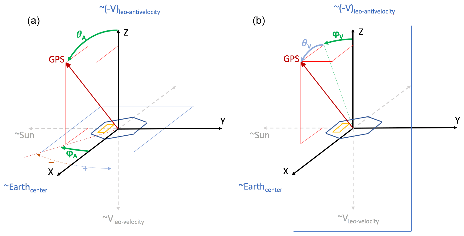
Figure 4Graphical sketch of the reference frames defined in the text. The same x, y, and z axes (fixed in the satellite body frame) are used to define both reference frames. (a) Antenna reference frame: the principal plane where the location of the GPS satellite is evaluated is the x–y plane, emphasized by a thin blue line; (b) velocity reference frame: the principal plane where the location of the GPS satellite is evaluated is the y–z plane, emphasized by a thin blue line. The approximate directions at which the different axes point to are specified for reference for the reader.
3.1.1 The antenna reference frame
The so-defined antenna reference frame is used for the antenna characterization. This reference frame is constructed on the x, y, and z axes defined above and is a spherical coordinate system. Therefore, is specified by a radial distance, a polar angle (or inclination), and an azimuthal angle. The radial distance corresponds to the distance between PAZ satellite and the tracked GPS satellite. The polar angle, or inclination (θA), corresponds to the angle between the z axis and the origin – the GPS vector. The azimuth angle (φA) corresponds to the projection of the inclination angle on the x–y plane, containing the origin and orthogonal to the zenith. The positive values of φA are defined such that the angle increases towards the positive y axis (angle φA has the same sign as y). The formal definitions of the angles are as follows:
This reference frame is sketched in Fig. 4a.
3.1.2 The velocity reference frame
It is also worth defining another reference frame, named here as the velocity reference frame, used in the RO community and used to define the parameters set in the RO receiver aboard PAZ. Differently from the antenna reference frame, whose reference plane is the plane containing the antenna, here the reference plane is the y–z one, which is parallel to the normal vector of the antenna and (pseudo-)tangential to the Earth's surface. Once the reference frame is defined, the azimuth (φV) and elevation (θV) angles can be defined as
This reference frame is sketched in Fig. 4b.
3.2 Antenna pattern characterization
To characterize the response of the antenna depending on the angle of incidence of the incoming radio waves, we use the φA and θA based on the relative positions of the GPS and the LEO, without taking into account the bending angle of the ray by the atmospheric refractive index gradients. The consequence is that θA will be overestimated due to the fact that the actual rays bend and arrive at the antenna as if they were coming from the limb of the Earth while the actual GPS position is below the Earth's surface. Since we only use the positions, i.e., straight rays, the θA spans further down than it really is.
First of all, we look at the effective antenna pattern of the SNR for both the H and V antennae (Fig. 5). The SNR antenna patterns show a different behavior in the H and V antennae. Based on the measurements made in an anechoic chamber before the installation of the antenna (shown in Cardellach et al., 2014, Fig. 5 – top and center panels), the H antenna should perform slightly better than the V one and have a maximum gain centered at φ=0, decreasing towards the edges. However, we can see in Fig. 5 how the installation of the metallic structure changed this pattern. Now, the best performance is achieved by the V antenna, although the maximum gain is centered around ∘. The lower performance at ∘ is most likely due to the blockage by the metallic structure. Also, most of the data with ∘ do not pass the quality controls, and therefore there are fewer data available to contribute to the antenna pattern. On the other hand, the H antenna exhibits an irregular pattern, with a sinusoidal-like behavior along all the φA range. This behavior is consistent with the signal being affected by strong multipath.
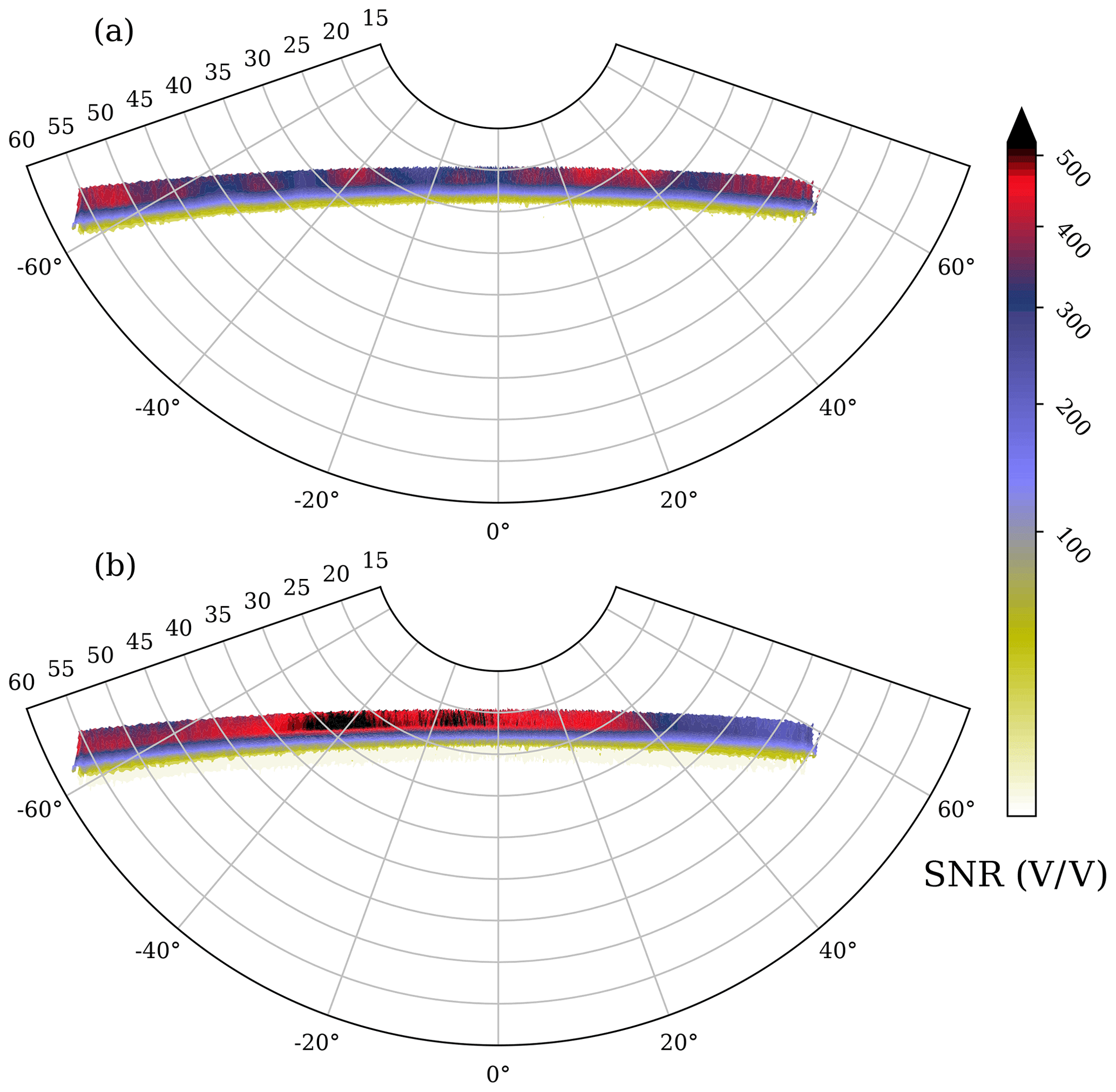
Figure 5Effective antenna pattern for the signal-to-noise ratio (color scale) at (a) the horizontal port and (b) the vertical port, as a function of azimuth (x axis) and elevation (y axis) in the antenna reference frame (φA, θA).
The SNR pattern shows how the metallic structure affects the signal, but what we are really interested in is in the ΔΦ pattern. This antenna pattern is shown in Fig. 6. We can also see how the ΔΦ antenna pattern changed with respect to the original one measured in the anechoic chamber (e.g., Cardellach et al., 2014, Fig. 5, bottom panel). The fact that we set ΔΦ=0 at 30 km makes the antenna pattern relative to that location. At 30 km height, the bending angle is small enough to consider that for a given azimuth, the elevation that corresponds to 30 km is very similar. Therefore, the antenna pattern characterizes the trends in the differential phase shift rather than the absolute values. The pattern of the phase difference arises from the combination of the patterns from the H and V antennae and is irregular. The antenna pattern is used to correct every single ΔΦ measurement, which is compared against the pattern for all the given (φA, θA) as detailed in Sect. 5.
Faraday rotation (Ω) in the ionosphere can introduce a differential phase shift between the H and V components (Tomás et al., 2018). It depends on the electron density (ne), the magnetic field (B), and the relative orientation of the propagation direction (r) and the magnetic field vector as follows:
where the constant is in international units, and the Faraday rotation is in radians. The Faraday rotation induces a rotation of the polarization axis of the ellipse described with a linear basis. If the electromagnetic wave is perfectly circularly polarized, this rotation does not induce a differential phase shift. However, if the wave is not circularly polarized, the rotation induces a ΔΦ between the H and V components. There are two instances that can lead to a non-circularly polarized wave in a situation like the one we are analyzing here, which are as follows:
-
The first is imperfect emission. Ideally, GPS satellites emit RHCP radio waves. However, it is not guaranteed that this emission is perfect, and some impurities are to be expected. Therefore, if the emission is not perfect, radio waves travel through the ionosphere, experiencing a ΔΦ that is proportional to the Faraday rotation (Tomás et al., 2018):
where m and Δ characterize the difference in the emitted wave from the perfect circular polarization, i.e., .
-
The second is after crossing precipitation. When the radio wave crosses precipitation, even if it were perfectly circularly polarized, it would experience a ΔΦ induced by the hydrometeors. Therefore, after the rain on its way to the receiver, it crosses the ionosphere being non-circularly polarized. This implies that the second part of the ionosphere (i.e., the Faraday rotation induced along the portion of the ionosphere that the ray crosses from its tangent point to the receiver, Ω2) induces a differential phase shift that depends on the ΔΦ induced by precipitation (here identified as ΔΦprecip):
Such expressions are thoroughly derived in Tomás et al. (2018). It is also shown in Tomás et al. (2018), based on simulations, that the effect of the Faraday rotation due to the impurities in the emission (Eq. 9) should be possible to correct, and the effect after crossing rain (Eq. 10) is small enough to not introduce substantial errors in the measurements because Ω2 is generally low.

Figure 6Antenna pattern for the ΔΦm as a function of azimuth (x axis) and elevation (y axis) in the antenna reference frame (φA, θA).
In the following section we analyze the observations based on the colocated electron density and magnetic field in order to infer whether the ionosphere is inducing any noticeable ΔΦ.
Faraday rotation for PAZ PRO events
First of all we need to know what the typical values of Faraday rotation along PRO rays are. We take two heights, 10 and 50 km, at which we evaluate the Faraday rotation using the colocated values of ne and B from IRI and IGRF. For every PRO, we compute the total Faraday rotation at 50 and 10 km and the second part of the Faraday rotation at 10 km. The histograms for all the cases are shown in Fig. 7.
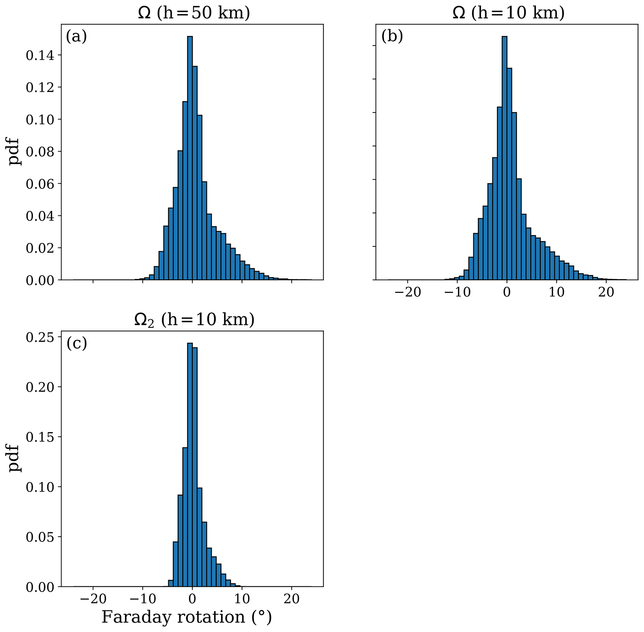
Figure 7Histograms for the Faraday rotation values. Panels (a) and (b) represent the histograms for the total Faraday rotation (Ω) evaluated at the ray with tangent point's height around (a) 50 km and (b) 10 km. In (c) there is the histogram for the second part of the Faraday rotation (Ω2), evaluated at the ray with tangent point's height of 10 km.
Summarizing Fig. 7, the total Faraday rotation has values between −12 and 20∘ and is between −6 and 10∘ for the portion of the Faraday rotation between the tangent point and the receiver. We have also seen that the maximum difference in total Faraday rotation between 50 and 10 km is as high as 3∘ and as low as −2∘. The difference of Ω between two heights determines the trend in ΔΦ that Faraday rotation could be inducing, assuming that the wave is not perfectly circularly polarized when it crosses the ionosphere. In Fig. 8 we show the trend in ΔΦ, understood as ΔΦ50 km−ΔΦ10 km, as a function of the Ω at 50 km (which in its turn determines the trend in Ω; the higher the Ω, the higher the trend). We can see that the trend in ΔΦ is imperceptible. This agrees with the simulations, which say that if there is a trend, it should be small (as high as 0.6 mm), depending on m and Δ that are unknown. In addition, m and Δ should change by transmitter and probably by time and transmitter orientation, which makes them impossible to infer. The same study as in Fig. 8 has been done separating the data by GPS transmitter, with no revealing results.
Regarding the effect of the ionosphere after the rays have crossed precipitation (e.g., Eq. 10), we can evaluate the error introduced in our measured ΔΦ with respect to ΔΦprecip. With the values shown in Fig. 7, we obtain that the measured ΔΦ is reduced by 6 % in the case of a Ω2∼10∘, which would be an extreme and rare situation. In the event that Ω2=20∘, the measured ΔΦ would be reduced to 25 % below the actual ΔΦprecip. Ninety percent of the observed Ω2 is confined between −3 and 4.7∘, which implies that the measured ΔΦ is reduced by 1.3 %. It is true that the ionospheric activity has been very low during the period the data were obtained (i.e., 2018–2019); therefore further analyses will be needed when solar activity increases.
Based on the actual values for Ω and Ω2, it is safe to assume that the effect of the ionosphere on the ΔΦ is generally negligible (below the noise level of the measurement) and only in a very few cases can have a minor effect. This corroborates the simulation study performed in Tomás et al. (2018) before the launch of the PAZ satellite. Nevertheless, the trend that is detected in ΔΦ (measured between 50 and 10 km), small in average, is corrected from the whole observation, regardless of whether it is an ionospheric effect or residuals from the first steps of the calibration of the observables.
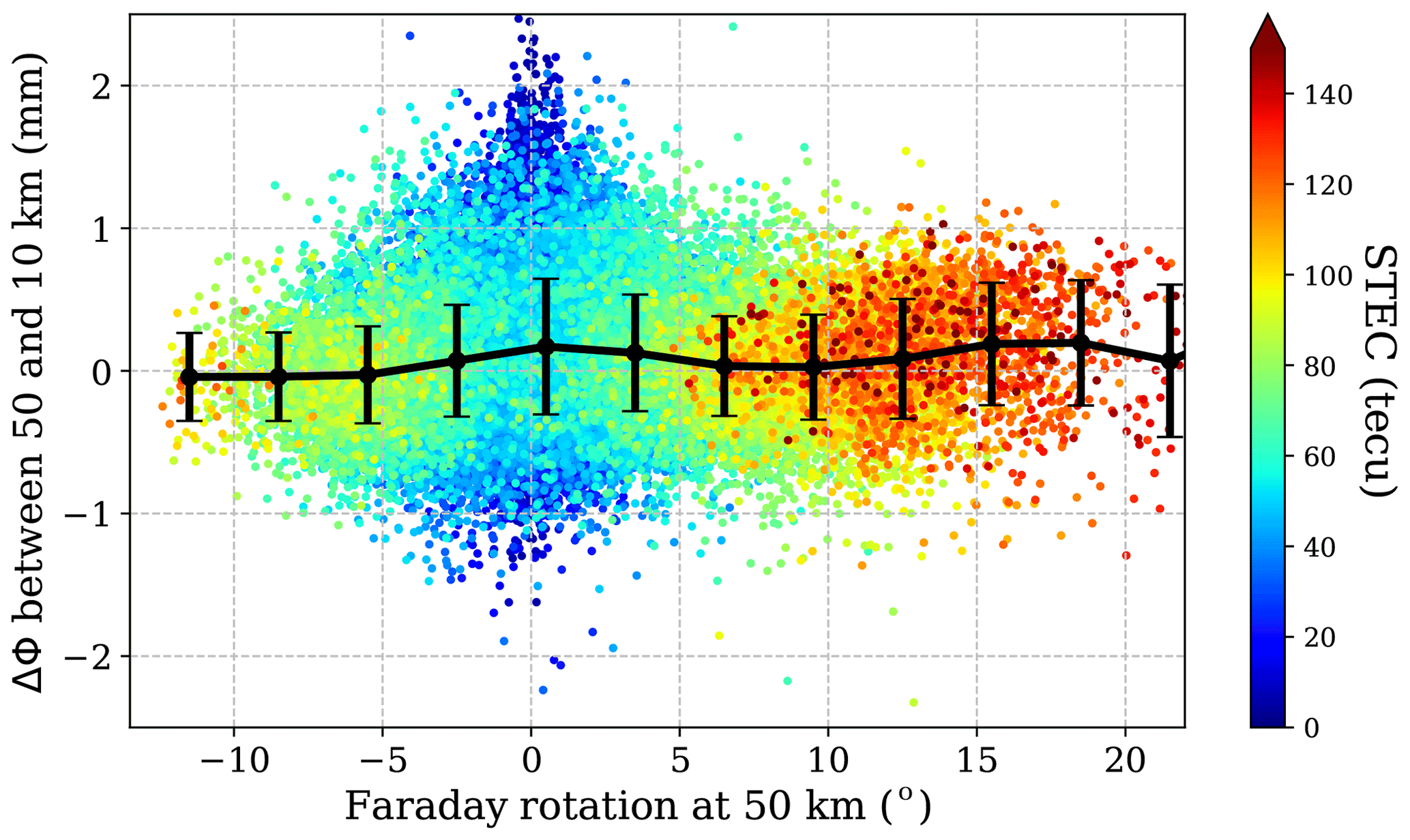
Figure 8Trend of ΔΦ(h) as a function of Faraday rotation. The ΔΦ is evaluated at the rays with tangent point's heights of 50 and 10 km, and the difference between them is plotted here as a function of Ω evaluated at the ray with tangent point's height of 50 km. The color of the points shows the integrated electron density content along the ray with tangent point's height of 50 km. Solid line is the mean, and the error bars are the standard deviation.
We have gone through the different, necessary steps before performing the calibration of the observables, from the acquisition of the signal to the antenna pattern characterization, and taken into account all the possible effects that can induce a differential phase shift, besides precipitation. The steps followed to calibrate the ΔΦ are identified and described in Fig. 9 and summarized below.
-
First is the acquisition of the signal. The incoming electromagnetic signal is collected at two independent linearly polarized antennae, orthogonal to each other, oriented to get the horizontal and the vertical components of the radio wave, simultaneously. The difference between the excess phase of both ports (H and V) gives us the observable (step 1 in Fig. 9), which is further corrected for remaining cycle slips (step 3) and set to 0 in the regions above where any precipitation is possible (step 4). The observations are obtained as a function of time, but having precise information about the location and relative orientation of both the GPS and the PAZ satellites we can link time to azimuth and elevation from the receiving antenna point of view so that we can obtain the measured differential phase shift as a function of such variables: ΔΦm(φA,θA). After the processing, time can also be linked to height, so we can have ΔΦm(h) as well (step 2).
-
Every PRO event is checked against precipitation (step 5). This allows us to group the events by rainy or non-rainy, where rainy means that there exists precipitation inside the potentially sensed region, and non-rainy means that no precipitation is present in the region. Furthermore, the colocated brightness temperature is used to further ensure that no precipitation was sensed by selecting those cases where the minimum Tb is warmer than 250 K. Hence, PRO events are linked to R (rain rate) and Tb.
-
The ionospheric conditions (i.e., electron density) and the Earth's magnetic field (both intensity and orientation) are evaluated at the trajectory points of each ray for all of the PRO observations in order to compute the undergone Faraday rotation (step 6). The total Faraday rotation Ω and the partial one (i.e., the Faraday rotation suffered by the ray from the tangent point to the receiver) Ω2 are linked to all PRO.
At this point, every ith PRO event has some variables associated with it,
Data linked to no rain and low ionospheric activity are used to build the antenna pattern ΔΦpattern(φ,θ) (step 7). And this antenna pattern is used to correct the whole dataset of observations (step 8) as follows:
where the subscript “c” stands for corrected.
The possible Faraday rotation effect, although expected to be small in general (e.g., see Sect. 4), is not fully corrected by this process. The antenna pattern characterization captures these ionosphere-induced trends and possible errors induced by the performance of the antenna. It is intentionally constructed with low ionospheric activity data so that it does not capture the stronger trends induced by the active ionosphere, since they can be different and have nothing to do with the relative angle at which they arrive at the antenna. Therefore, every is corrected for remaining possible linear trends present above 20 km (step 9) as follows:
where the linear trend is evaluated above 20 km and extrapolated to all heights. With this last step we obtain the calibrated ΔΦi(h). After the whole calibration, we expect that ΔΦi(h) is as similar to as possible, where is the differential phase shift induced only by precipitating hydrometeors. Note that the preliminary calibration in Cardellach et al. (2019) did not include steps 5 to 8.
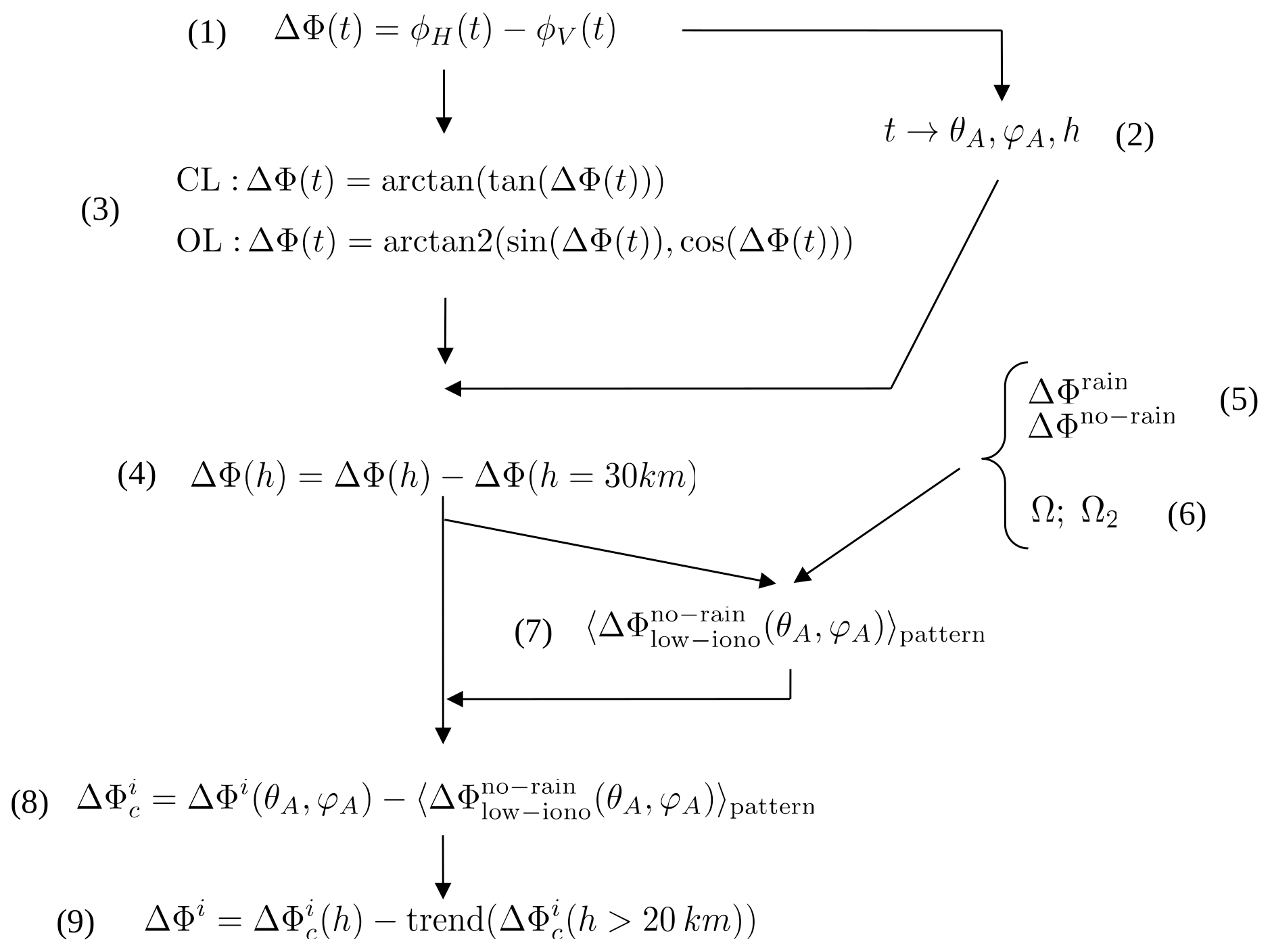
Figure 9Block diagram identifying and describing the steps followed during calibration: (1) start with the observable: phase difference between H and V; (2) map time into other variables; (3) do correction for remaining cycle slips; (4) set the zero level at 30 km; (5) and (6) do colocations with precipitation information and ionospheric activity; (7) use accumulation of free-of-rain and low-ionospheric activity measurements to create the effective antenna pattern; (8) subtract the effective antenna pattern to each measurement; and (9) correct for remaining trends.
Smoothing of the signal
Once we have calibrated the signal, we smooth it to reduce the uncertainty. PRO are acquired at 50 Hz, but for the purposes of detecting precipitation it is enough to have measurements at 1 s resolution. While the smoothing reduces the standard error by accounting for more samples for each measurement (e.g., we use 50 points obtained at 50 Hz to represent the measurement at 1 s resolution), its counterpart is that it reduces the vertical resolution of the observation, being about a few hundred meters after smoothing. Generally, a simple running average window would be applied to perform the smoothing. However, here we want to stress the fact that the measurements with a higher signal-to-noise ratio have less uncertainty. The uncertainty in the phase measurement is determined by the SNR of each measurement (e.g., Cardellach et al., 2014), so the uncertainty in the ΔΦ comes from the propagation of such an error from both H and V ports. Therefore, instead of a simple average, here we perform a 1 s weighted average, where the weight is represented by the SNR value so that values of ΔΦ associated with a higher SNR contribute more than those associated with a lower SNR. In this case, since we are combining both the measurements from the H and V ports, the SNR that we use for the weighted average is . The SNR values are limited so that only those above 10 V∕V contribute to the mean.
The smoothed calibrated measurements 〈ΔΦ〉1s are to be validated against IMERG. For comparison and standardization purposes, we interpolate the 〈ΔΦ〉1s for a 100 m grid, spacing profiles from 0 to 30 km: ΔΦ(h100 m). For these profiles we can perform the mean and the standard deviation at each altitude. First of all, we group them by their linked precipitation and brightness temperature: (1) no precipitation (R=0 mm h−1 and Tb>250 K), (2) precipitation (R>0.1 mm h−1), and (3) heavy precipitation (R>1 mm h−1). For these three groups we compute the mean and standard deviation as a function of height. In Fig. 10 we show the results. We can see how for the no-precipitation group the ΔΦ(h100 m) averages to 0 for the whole vertical profile (by design), and the standard deviation, σΔΦ(h), increases with decreasing altitudes. In the right panel of Fig. 10 we show a more detailed profile of the σΔΦ(h).
The first remark is that σΔΦ(h)=1.2 mm at 2 km of height. This is better than the study performed in Cardellach et al. (2019), which is expected since here we calibrated the signal using the antenna pattern and we have performed the weighted average smoothing. It is also very close to the theoretically predicted sensitivity in Cardellach et al. (2014). The second noticeable feature is the peak in σΔΦ(h) around 7 km. This feature is due to instrumental effects in some occultations near the CL to OL transition and is an open issue under investigation. Finally, a small negative bias is observed within the lower 1 km. As we have explained in Sect. 2.1, the results below 2 km have to be treated with caution, since many uncertainties (tangent height determination, atmospheric multipath, etc.) come into play.
Still in Fig. 10, the precipitation and heavy precipitation groups (blue and red, respectively) exhibit large positive values below 10 km, although positive values start to be noticeable below 15 km. The positive peaks are well above the standard deviation of the no-precipitation group, indicating sensitivity to precipitation and consistent with Cardellach et al. (2019).
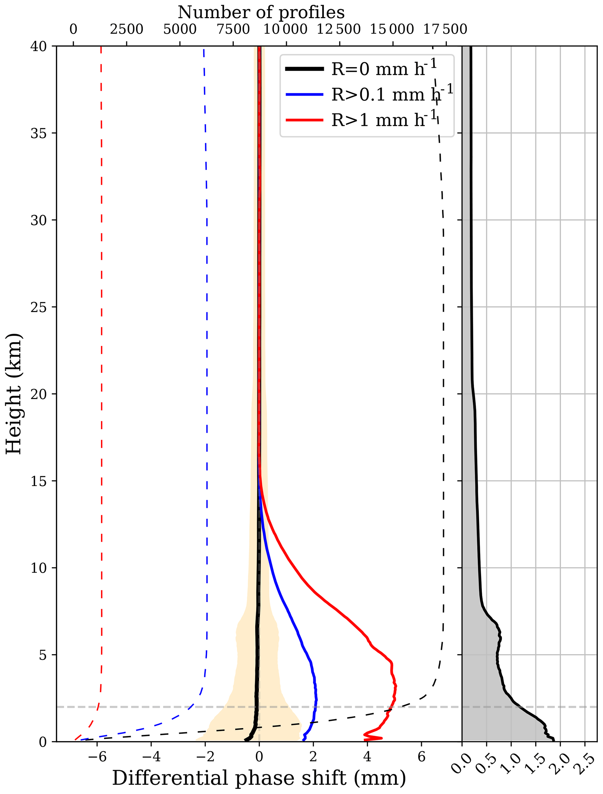
Figure 10Mean (solid black line) and standard deviation (orange shaded) of ΔΦ(h100 m) as a function of height for the PRO events collected under no rain conditions. The solid blue and red lines show the mean of ΔΦ(h100 m) as a function of height for the PRO events collected under R>0.1 and R>1 mm h−1, respectively. The dashed lines show the number of collected profiles (top axis) as a function of height corresponding to each group (no precipitation, R>0.1 and R>1 mm h−1). The right side panel shows a more detailed vertical profile of the standard deviation σΔΦ(h) for the PRO events collected under no rain conditions (gray shaded area). The dashed gray horizontal line indicates the 2 km altitude.
As it was done in Cardellach et al. (2019), we can characterize each PRO observation by a single value derived from the ΔΦ(h100 m). This is done by averaging ΔΦ(h100 m) between two different heights. In this case, we use 0 to 10 km, obtaining 〈ΔΦ〉0–10 km. To associate one single measurement is useful to validate the observations against the precipitation products. In Fig. 11 we show 〈ΔΦ〉0–10 km as a function of the associated rain rate. The binned mean (solid line) shows how 〈ΔΦ〉0–10 km values tend to increase as R increases, exhibiting sensitivity to the intensity of precipitation.
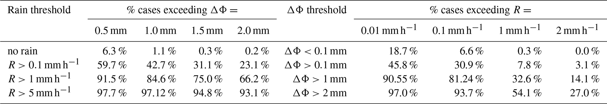
It is also interesting to assess the percentage of cases that exceed a certain threshold of 〈ΔΦ〉0–10 km given a precipitation value. This sets a detectability metric of 〈ΔΦ〉0–10 km based on the colocations, and we can assess the quantity of false positives. We show the results in the Fig. 12a. In this plot we see how for no precipitation, there are 6 % of cases that exceed 〈ΔΦ〉0–10 km=0.5 mm, while there are almost no cases exceeding 1 mm (or higher). This tells us that the rate of false positives is very low, and depending on the threshold we choose, is almost nonexistent. The same plot shows the percentage of cases exceeding different thresholds of 〈ΔΦ〉0–10 km (represented by different colors; see legend inset). For example, as we can see in Table 1, 85 % of the cases exceed 〈ΔΦ〉0–10 km=1 mm when precipitation is heavier than 1 mm h−1, and more than 93 % of the cases exceed 〈ΔΦ〉0–10 km=2 mm when precipitation exceeds 5 mm h−1.
In the same way, we can assess which percentage of cases exceeds certain precipitation given a 〈ΔΦ〉0–10 km. This is shown in Fig. 12b. In this way we can assess the false negatives and see how likely it is to detect precipitation given a 〈ΔΦ〉0–10 km. The leftmost region of the plot shows the fraction of cases exceeding certain precipitation when the observed 〈ΔΦ〉0–10 km is small (i.e., smaller than 0.1 mm). For a precipitation threshold of 0.01 mm h−1, this fraction is around 19 %, while for precipitation heavier than 1 mm h−1 (and higher) it is almost 0 (see Table 1). We can also see how, for example, when the measured 〈ΔΦ〉0–10 km is larger than 1 mm, there is an 81 % chance of measuring precipitation with 0.1 mm h−1 or higher.
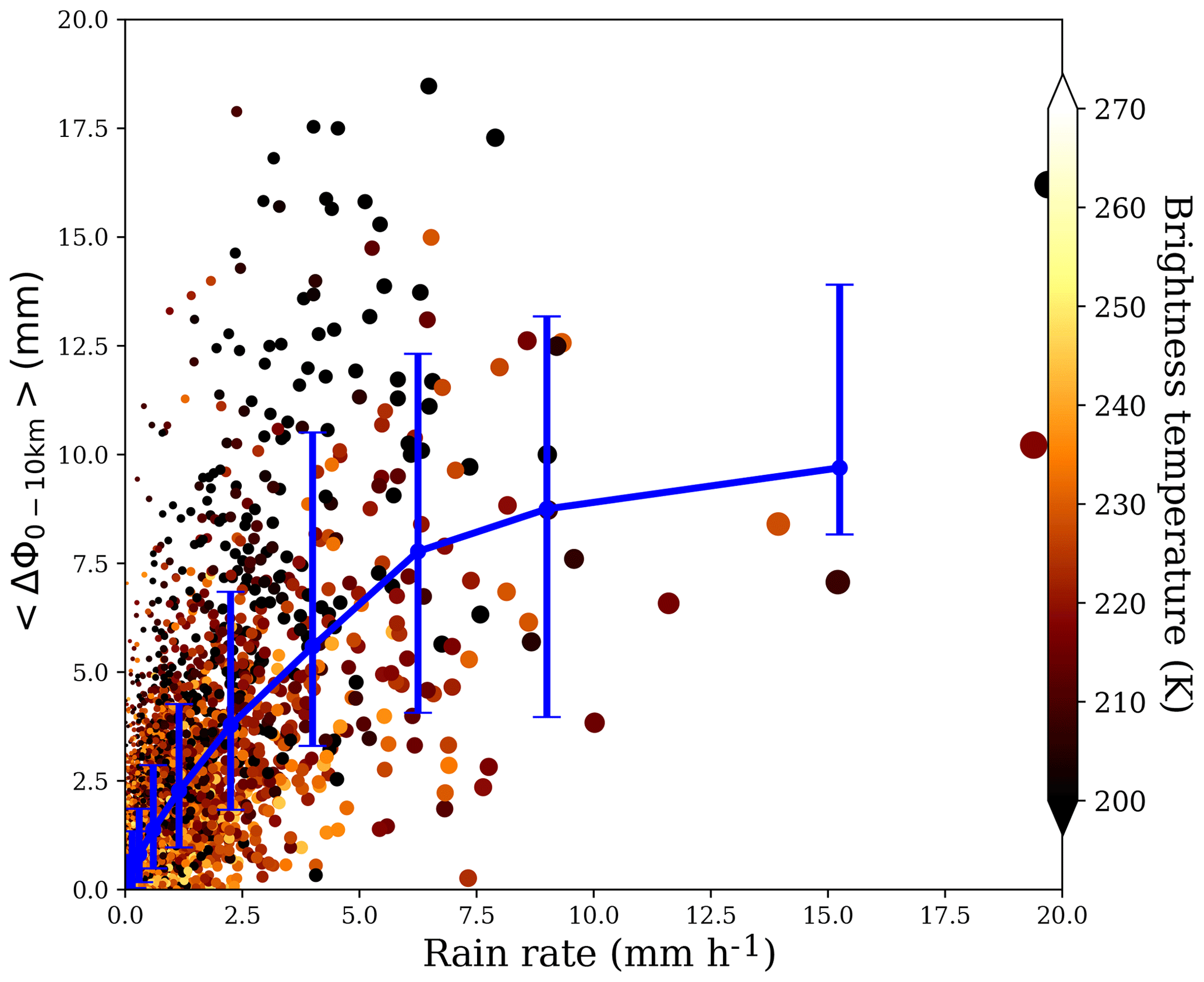
Figure 11〈ΔΦ〉0–10 km as a function of rain rate. The color indicates the minimum Tb for every case. The solid blue line represents the mean of all the data inside precipitation bins. The error bars comprise 85 % of the data.
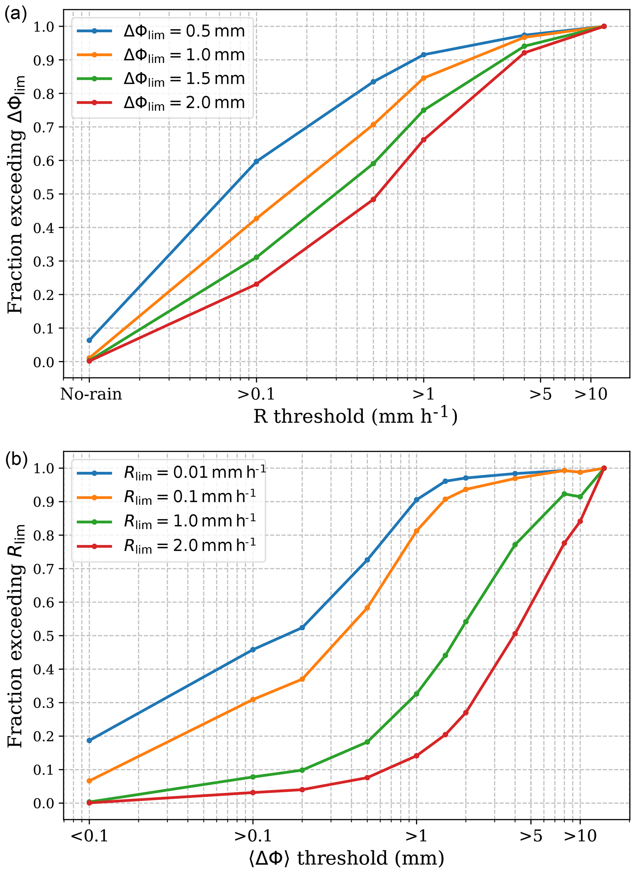
Figure 12(a) Fraction of cases exceeding certain 〈ΔΦ〉0–10 km value (blue: 0.5 mm; orange: 1.0 mm; green: 1.5 mm; and red: 2.0 mm) as a function of the associated precipitation threshold. (b) Fraction of cases exceeding a certain precipitation value (blue: 0.01 mm h−1; orange: 0.1 mm h−1; green: 1.0 mm h−1; and red: 2.0 mm h−1) as a function of measured 〈ΔΦ〉0–10 km threshold.
6.1 Variability by transmitter
As it has been mentioned in Sect. 4.1, the way the signal is emitted from the GPS transmitter can also have an effect on ΔΦ, particularly if the emission is not perfectly RHCP. However, this effect should be small (e.g., see Fig. 8). Here we investigate whether different transmitters have similar statistics (as we expect) or not. To do so we reproduce the analysis done to generate Fig. 10, grouping the data by transmitter. The results for the ΔΦ(h100 m) and σΔΦ(h), evaluated at 3 km of altitude, are shown in Fig. 13.
The results for the different transmitters (also separated here by block, i.e., the version of satellite) show how the ΔΦ(h100 m) and σΔΦ(h) are consistent with the global mean and σ, showing no dependence on the transmitter.
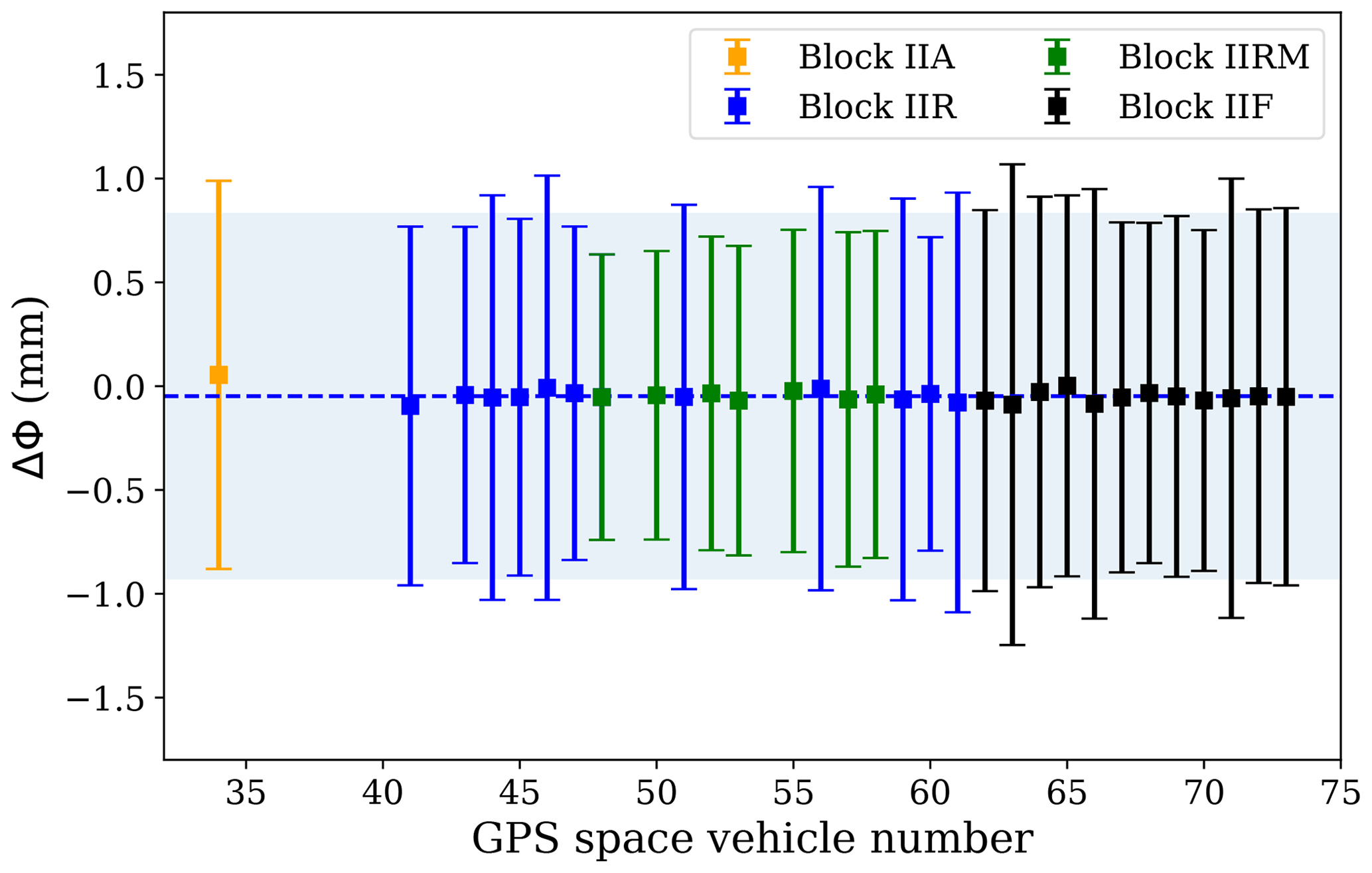
Figure 13Mean and standard deviation of the ΔΦ measurements for the rain-free cases, at a height of 3 km, as a function of the transmitter (i.e., the GPS space vehicle number). The blue dashed line and the light blue shadow represent the mean and standard deviation of the whole dataset of rain-free cases. Different colors for the error-bar points represent different GPS satellite blocks, as indicated in the legend.
6.2 Cross-polarization isolation
The metallic structure could have worsened the overall performance of the polarimetric antenna by reducing the cross-polarization isolation. Some simulations of how it affects the ΔΦprecip with respect to the measured one are performed in order to assess this effect. The transmission matrix that represents the antenna can be expressed as
For a good cross-polarization isolation (e.g., dB), the terms ahv and avh can be approximated to 0. In this case, the cross-polarization isolation is not known due to the disturbance included by the metallic structure, but simulations provided by Hisdesat suggest a cross-polarization isolation between −15 and −20 dB, which means that ahv and avh cannot be neglected.
We have performed simulations assuming , where a=0.17 (corresponding to −15 dB, i.e., conservative approach) and that φ can take any value. We compare the ΔΦ that we would measure without the antenna with the ΔΦ if the antenna is present, and this introduces a differential phase shift between the H and V components from the poor cross-polarization isolation. The simulations are performed accounting different ΔΦprecip and different values for Ω2. The results, plotted in Fig. 14, show that the ratio between the measured ΔΦ and the actual ΔΦprecip can be as high as 15 % (only the results for Ω2=10∘ are shown). However, the maximum variance comes from the variation in φ, which is unknown and probably not constant. Averaging over all the results for different φ values, the average ratio is 1, and the standard deviation is around 7 %. It is also important to notice that the variability induced by Ω2 is also included; therefore the values of the ratio include both the ionosphere effect and the poor cross-polarization isolation.

Figure 14Ratio between the measured ΔΦ and the precipitation-induced ΔΦprecip as a function of the complex angle φ in aeiφ, for a=17 and for different values of precipitation. The value of Ω2=10 ∘. The precipitation values range between an induced ΔΦprecip of 0.1 mm (bluer) to 15 mm (redder).
In this paper we have described the steps and the procedure followed to calibrate and validate the PRO ΔΦ observable. The calibration of the observable is a critical step in the mission, which has to ensure the quality and robustness of the observables. Being the first time that these kind of measurement are being obtained, the validation of the observables is also very important, since it will establish a reference for future missions.
First of all, the calibration of the signal has been performed by using the existing data to characterize the antenna pattern. Such an exercise is more important than it should be due to the interferences introduced by a metallic adapter that had to be installed above the antenna, to adapt the satellite to a new launcher. In order to not introduce features coming from the kind of signals that we aim to detect (i.e., precipitation-induced ΔΦ), the characterization is performed using only data collected in rain-free scenarios. Furthermore, ionosphere could introduce a small ΔΦ through the Faraday rotation; hence observations that have sensed regions with high ionospheric activity are also discarded for the calibration. Finally, the antenna pattern is then used to correct all the observations, regardless of precipitation or ionospheric activity.
The corrected observations are thoroughly validated. First, we have performed the statistical analysis of both no-precipitation and precipitation groups of observations. The mean and standard deviation of the no-precipitation profiles set the quality of the observations. Without the presence of precipitation, what remain are the uncertainties and the unsought effects, so the standard deviation tells us the noise level of the measurement. Inside the noise level we assume that we can have the thermal noise arising from the phase measurements, residual effect from the calibration, and cross-polarization terms from the non-perfect isolation of the antenna. In spite of that, the vertical profile of the standard deviation (see Fig. 10) shows a good noise level (below 1.5 mm above 2 km, below 1 mm above 3 km, and better than 0.5 mm above 8 km), close to what was predicted in the initial sensitivity studies for the experiment (Cardellach et al., 2014). It is also confirmed that the Faraday rotation effect on the final observable is small and that the transmitter polarization impurities are negligible.
In addition, the mean ΔΦ measurements as a function of height for the precipitation groups exhibit a clear and distinguishable positive peak, reaching altitudes above 10 km and exceeding ΔΦ=5 mm in the lower layers for the group comprising the precipitation rates larger than 1 mm h−1. This clearly indicates that the measurement is sensitive to precipitation, corroborating the initial findings in Cardellach et al. (2019). It also indicates that the measurement might be sensitive to higher-altitude phenomena other than precipitation, such as ice or melting particles, usually present above the freezing level and particularly in the heavy tropical precipitation structures.
Further validation is performed using the vertical average of ΔΦ(h100 m) between the surface level and 10 km for each individual observation, defined as 〈ΔΦ〉0–10 km. This allows us to use single values rather than vertical profiles associated with each observation for simplicity in the validation process. Using this approach we can assess the variation in 〈ΔΦ〉0–10 km with increasing R (see Fig. 11). The fact that 〈ΔΦ〉0–10 km keeps increasing as R increases tells us that ΔΦ measurements are sensitive to not only precipitation but also its intensity. Here we want to remind readers that in this context precipitation intensity means higher mean rain rate integrated for the sensed region (see Sect. 2.3), which could either mean more intense precipitation, a larger precipitation cell, or both.
The same ΔΦ(h100 m) measurement is used to evaluate the detectability of precipitation for different thresholds (see Fig. 12). For example, we can state that more than 80 % of the cases with R>1 mm h−1 exceed ΔΦ(h100 m)=1.5 mm. In a different, yet equivalent, way we can state that 50 % of the cases with ΔΦ(h100 m)>2 mm exceed a R=1 mm h−1, but more than 90 % will have R>0.1 mm h−1. Therefore, the detectability will depend on the threshold that one sets. On the other hand, the same study shows low values for false positives and false negatives regardless of the chosen threshold. Setting the thresholds towards the heavier rain range (although heavy rain is not qualitatively defined here) decreases the false positives and negatives dramatically, exhibiting a very good performance of the technique in detecting rain. It is important here to emphasize the fact that we are evaluating the performance in detecting rain rather than quantifying its rate, and the validation in the context of this paper confirms this capability.
These results confirm the potential of the PRO technique to provide joint measurements of precipitation and thermodynamics, becoming a very valuable and unique technique. Further analyses need to be done in order to address the quantification of precipitation, as well as to exploit this and other scientific applications.
PAZ data will be available at https://paz.ice.csic.es/ (last access: 18 March 2020) and https://genesis.jpl.nasa.gov/genesis/ (last access: 18 March 2020). NCEP/CPC infrared brightness temperature datasets (https://doi.org/10.5067/P4HZB9N27EKU; Janowiak et al., 2017) and IMERG precipitation datasets (https://doi.org/10.5067/GPM/IMERG/3B-HH/06; Huffman et al., 2019) are available from NASA Goddard Earth Sciences Data and Information Services Center (GES DISC).
All coauthors contributed to the design of the analysis and interpretation of the results. RP led the data analysis and the writing. COA, BI, and KNW performed the inversion of the raw data. RP, COA, FJT, MTJ, KNW, and EC performed the colocations, calibration, and validation of the data. EC is the P.I. of the mission.
The authors declare that they have no conflict of interest.
Ramon Padullés' research was supported by an appointment to the NASA Postdoctoral Program at the Jet Propulsion Laboratory, administered by Universities Space Research Association under contract with NASA. The JPL coauthors acknowledge support from the NASA US Participating Investigator (USPI) program. The work conducted at ICE-CSIC/IEEC was supported by the Spanish Ministry of Science, Innovation and Universities. Part of Estel Cardellach's contribution has been supported by the Radio Occultation Meteorology Satellite Application Facility (ROM SAF), which is a decentralized operational RO processing center under EUMETSAT. The authors want to thank the two anonymous reviewers for their valuable comments that helped to improve the paper.
This research has been supported by NASA ROSES Earth Science U.S. Participating Investigator grant no. 14-ESUSPI14-0014; Spanish Ministry of Science, Innovation and Universities (RTI2018-099008-B-C22); and EUMETSAT (ROM SAF CDOP3).
This paper was edited by Joanna Joiner and reviewed by two anonymous referees.
Ao, C. O., Meehan, T. K., Hajj, G. A., and Mannucci, A. J.: Lower troposphere refractivity bias in GPS occultation retrievals, J. Geophys. Res., 108, 1–16, https://doi.org/10.1029/2002JD003216, 2003. a
Ao, C. O., Hajj, G. A., Meehan, T. K., Dong, D., Iijima, B. A., Mannucci, A. J., and Kursinski, E. R.: Rising and setting GPS occultations by use of open-loop tracking, J. Geophys. Res.-Atmos., 114, 1–15, https://doi.org/10.1029/2008JD010483, 2009. a
Bilitza, D., Altadill, D., Truhlik, V., Shubin, V., Galkin, I., Reinisch, B., and Huang, X.: International Reference Ionosphere 2016: From ionospheric climate to real-time weather predictions, Space Weather, 15, 418–429, https://doi.org/10.1002/2016SW001593, 2017. a
Cardellach, E., Tomás, S., Oliveras, S., Padullés, R., Rius, A., de la Torre-Juárez, M., Turk, F. J., Ao, C. O., Kursinski, E. R., Schreiner, W. S., Ector, D., and Cucurull, L.: Sensitivity of PAZ LEO Polarimetric GNSS Radio-Occultation Experiment to Precipitation Events, IEEE T. Geosci. Remote, 53, 190–206, https://doi.org/10.1109/TGRS.2014.2320309, 2014. a, b, c, d, e, f, g, h
Cardellach, E., Padullés, R., Tomás, S., Turk, F. J., de la Torre-Juárez, M., and Ao, C. O.: Probability of intense precipitation from polarimetric GNSS radio occultation observations, Q. J. Roy. Meteor. Soc., 144, 206–220, https://doi.org/10.1002/qj.3161, 2018. a
Cardellach, E., Oliveras, S., Rius, A., Tomás, S., Ao, C. O., Franklin, G. W., Iijima, B. A., Kuang, D., Meehan, T. K., Padullés, R., de la Torre-Juárez, M., Turk, F. J., Hunt, D., Schreiner, W. S., Sokolovskiy, S. V., Van Hove, T., Weiss, J. P., Yoon, Y., Zeng, Z., Clapp, J., Xia-Serafino, W., and Cerezo, F.: Sensing heavy precipitation with GNSS polarimetric radio occultations, Geophys. Res. Lett., 46, 1024–1031, https://doi.org/10.1029/2018GL080412, 2019. a, b, c, d, e, f, g, h, i, j, k
Fjeldbo, G., Kliore, A., and Eshleman, V. R.: The Neutral Atmosphere of Venus as Studied with the Mariner V Radio Occultation Experiments, Astron. J., 76, 123–140, https://doi.org/10.1086/111096, 1971. a
Gorbunov, M. E.: Canonical transform method for processing radio occultation data in the lower troposphere, Radio Sci., 37, 1–9, https://doi.org/10.1029/2000RS002592, 2002. a
Hajj, G. A., Kursinski, E. R., Romans, L. J., Bertiger, W. I., and Leroy, S. S.: A Technical Description of Atmospheric Sounding By Gps occultation, J. Atmos. Sol.-Terr. Phy., 64, 451–469, https://doi.org/10.1016/S1364-6826(01)00114-6, 2002. a, b, c
Huffman, G. J., Stocker, E. F., Bolvin, D. T., Nelkin, E. J., Tan, J.: GPM IMERG Final Precipitation L3 Half Hourly 0.1 degree x 0.1 degree V06, Greenbelt, MD, Goddard Earth Sciences Data and Information Services Center (GES DISC) https://doi.org/10.5067/GPM/IMERG/3B-HH/06, 2019. a, b
Janowiak, J., Joyce, B., and Xie, P.: NCEP/CPC L3 Half Hourly 4km Global (60S–60N) Merged IR V1, Greenbelt, MD, Goddard Earth Sciences Data and Information Services Center (GES DISC), https://doi.org/10.5067/P4HZB9N27EKU, 2017. a, b
Kursinski, E. R., Hajj, G. A., Schofield, J. T., Linfield, R. P., and Hardy, K. R.: Observing Earth's atmosphere with radio occultation measurements using the Global Positioning System, J. Geophys. Res., 102, 23429–23465, https://doi.org/10.1029/97JD01569, 1997. a
Murphy, M. J., Haase, J. S., Padullés, R., Chen, S. H., and Morris, M. A.: The potential for discriminating microphysical processes in numerical weather forecasts using airborne polarimetric radio occultations, Remote Sens., 11, U2048–U2072, https://doi.org/10.3390/rs11192268, 2019. a
Padullés, R., Cardellach, E., Wang, K.-N., Ao, C. O., Turk, F. J., and de la Torre-Juárez, M.: Assessment of global navigation satellite system (GNSS) radio occultation refractivity under heavy precipitation, Atmos. Chem. Phys., 18, 11697–11708, https://doi.org/10.5194/acp-18-11697-2018, 2018. a
Sokolovskiy, S. V., Rocken, C., Hunt, D. C., Schreiner, W. S., Johnson, J. M., Masters, D., and Esterhuizen, S.: GPS profiling of the lower troposphere from space: Inversion and demodulation of the open-loop radio occultation signals, Geophys. Res. Lett., 33, 1–5, https://doi.org/10.1029/2006GL026112, 2006. a
Thébault, E., Finlay, C. C., Beggan, C. D., Alken, P., Aubert, J., Barrois, O., Bertrand, F., Bondar, T., Boness, A., Brocco, L., Canet, E., Chambodut, A., Chulliat, A., Coïsson, P., Civet, F., Du, A., Fournier, A., Fratter, I., Gillet, N., Hamilton, B., Hamoudi, M., Hulot, G., Jager, T., Korte, M., Kuang, W., Lalanne, X., Langlais, B., Léger, J.-M., Lesur, V., Lowes, F. J., Macmillan, S., Mandea, M., Manoj, C., Maus, S., Olsen, N., Petrov, V., Ridley, V., Rother, M., Sabaka, T. J., Saturnino, D., Schachtschneider, R., Sirol, O., Tangborn, A., Thomson, A., Tøffner-Clausen, L., Vigneron, P., Wardinski, I., and Zvereva, T.: International Geomagnetic Reference Field: the 12th generation, Earth Planet. Space, 67, 79, https://doi.org/10.1186/s40623-015-0228-9, 2015. a, b
Tomás, S., Padullés, R., and Cardellach, E.: Separability of Systematic Effects in Polarimetric GNSS Radio Occultations for Precipitation Sensing, IEEE T. Geosci. Remote, 56, 4633–4649, https://doi.org/10.1109/TGRS.2018.2831600, 2018. a, b, c, d, e, f, g
Turk, F. J., Padullés, R., Ao, C. O., de la Torre-Juárez, M., Wang, K. N., Franklin, G. W., Lowe, S. T., Hristova-Veleva, S. M., Fetzer, E. J., Cardellach, E., Kuo, Y.-H., and Neelin, J. D.: Benefits of a closely-spaced satellite constellation of atmospheric polarimetric radio occultation measurements, Remote Sens., 11, 2399, https://doi.org/10.3390/rs11202399, 2019. a