the Creative Commons Attribution 4.0 License.
the Creative Commons Attribution 4.0 License.
 | 30 Mar 2020
InnFLUX – an open-source code for conventional and disjunct eddy covariance analysis of trace gas measurements: an urban test case
Marcus Striednig
Martin Graus
Tilmann D. Märk
Thomas G. Karl
We describe and test a new versatile software tool for processing eddy covariance and disjunct eddy covariance flux data. We present an evaluation based on urban non-methane volatile organic compound (NMVOC) measurements using a proton transfer reaction quadrupole interface time-of-flight mass spectrometer (PTR-QiTOF-MS) at the Innsbruck Atmospheric Observatory. The code is based on MATLAB® and can be easily configured to process high-frequency, low-frequency and disjunct data. It can be applied to a wide range of analytical setups for NMVOC and other trace gas measurements, and is tailored towards the application of noisy data, where lag time corrections become challenging. Several corrections and quality control routines are implemented to obtain the most reliable results. The software is open source, so it can be extended and adjusted to specific purposes. We demonstrate the capabilities of the code based on a large urban dataset collected in Innsbruck, Austria, where three-dimensional winds and ambient concentrations of NMVOCs and auxiliary trace gases were sampled with high temporal resolution above an urban canopy. Concomitant measurements of 12C and 13C isotopic NMVOC fluxes allow testing algorithms used for determination of flux limits of detection (LOD) and lag time analysis. We use the high-frequency NMVOC dataset to generate a set of disjunct data and compare these results with the true eddy covariance method. The presented analysis allows testing the theory of disjunct eddy covariance (DEC) in an urban environment. Our findings confirm that the disjunct eddy covariance method can be a reliable tool, even in complex urban environments when fast sensors are not available, but that the increase in random error impedes the ability to detect small fluxes due to higher flux LODs.
- Article
(2222 KB) - Full-text XML
-
Supplement
(790 KB) - BibTeX
- EndNote


Eddy covariance (EC) is the method of choice for most micrometeorological studies of turbulent fluxes (e.g., Dabberdt et al., 1993; Aubinet et al., 2012). It has been extensively used in atmospheric sciences (e.g., Horst et al., 2004; Oncley et al., 2007; Patton et al., 2011) and biogeochemistry, e.g., Ameriflux, https://ameriflux.lbl.gov/ (last access: 22 March 2020); Euroflux, http://www.europe-fluxdata.eu/icos (last access: 22 March 2020) (Baldocchi et al., 1988; Fowler et al., 2009; Aubinet et al., 2012; Rannik et al., 2012; Ducker et al., 2018). The use of EC for atmosphere–surface exchange measurements is widespread and a number of commercial, freely distributed closed- and open-source codes for the analysis of EC data are available (e.g., Fratini and Mauder, 2014; Mauder et al., 2008, Metzger et al., 2017).
The basic concept of the eddy covariance method is derived from the conservation equation for a scalar s:
where D is the molecular diffusivity and Q is the chemical source and sink term (e.g., Stull, 1988).
Assuming horizontal homogeneity, all terms with horizontal derivatives will disappear.
Horizontal homogeneity at a flat surface also leads to vertical wind speed w to be 0, as the surface w is 0 and
where horizontal derivatives are 0. Further, if the chemical lifetime of the trace gas in question is much longer than the turbulent mixing timescale (Rinne and Ammann, 2012), the source term Q vanishes as well. Thus, we are left with two terms we can integrate from surface (z=0) to measurement height (z=h),
leading to
Noticing that the turbulent flux, , is orders of magnitude higher than the diffusive flux at typical flux measurement height (1–30 m) and that the turbulent flux at the surface goes to 0 as the vertical movements go to 0, we are left with
Turbulent flux at the measurement height h equals the diffusive surface flux, which we are usually interested in. There are different formulations of this, e.g., expressing biological sources as term Q, but they will lead to a similar final result in which the turbulent flux equals the sources below the measurement level.
In the past EC has been largely restricted to a limited number of species (e.g., H2O, CO2, CH4) due to the requirement of fast and highly accurate sensors (ideally sampling frequencies > 10 Hz). For reactive trace gases (such as non-methane volatile organic compounds, NMVOCs) that participate in air chemistry, instruments capable of EC have been much more limited (Guenther and Hills, 1998; Karl et al., 2001). However, owing to advances in mass spectrometry (Hansel et al., 1995; de Gouw et al., 2003; Jordan et al., 2009; Graus et al., 2010; Blomquist et al., 2010) and optical techniques (Kroon et al., 2007; Ammann et al., 2012; di Gangi et al., 2011; Muller et al., 2009), EC for reactive trace gases has recently become more tractable. A number of studies have used these new techniques to investigate emission and deposition processes of reactive gases (e.g., Karl et al., 2001, 2002, 2010; Velasco et al., 2005, 2009; Langford et al., 2009; Ruuskanen et al., 2011; Park et al., 2013; Nguyen et al., 2015) and aerosols (e.g., Nemitz et al., 2008; Farmer et al., 2013; Deventer et al., 2015). Compared to conserved tracers (e.g., CO2, H2O), reactive gases can potentially also be oxidized in the atmosphere and be converted from the point of emission (street canyon) to the point of measurement (e.g., tower). This issue is particularly relevant for the triad, where the chemical interconversion timescale is on the order of 100–200 s. The vertical turbulent mixing timescale for a typical friction velocity of 0.5 m s−1 and measurement height of approximately 40 m above street level in Innsbruck is ∼200 s. This is short compared to the atmospheric chemical lifetime of most NMVOCs. For example, the chemical lifetime of isoprene, one of the fastest-reacting NMVOCs, is about 30 min. While a minor issue for the present dataset, the chemical reactivity of NMVOCs might play a more important role on very tall towers above urban areas. Urban NMVOC flux measurements were first investigated by Velasco et al. (2005), who investigated NMVOC sources in Mexico City. Depending on available NOx, NMVOCs fuel tropospheric ozone formation and are considered a prime target for air pollution management. Unlike for CO2 (Christen et al., 2014), urban NMVOC flux data are still scarce. Spotted measurements have been reported for Mexico City (Velasco et al., 2005), London and Manchester (Langford et al., 2009, 2010), Helsinki (Rantala et al., 2016) and Innsbruck (Karl et al., 2018). The importance of investigating urban emission sources of NMVOCs has recently been highlighted by McDonald et al. (2018), who argue that volatile chemical products are emerging as largest petrochemical source of urban NMVOC emissions. New technological improvements make it now feasible to perform urban flux measurements of a wide range of NMVOCs. A milestone in atmospheric sciences for the analysis of trace gases and aerosols has been achieved in the last couple of years through the introduction of time-of-flight mass spectrometers (TOF-MS) (DeCarlo et al., 2006; Jordan et al., 2009; Graus et al., 2010). Chemical ionization methods coupled to time-of-flight mass spectrometers are becoming sensitive enough to simultaneously measure a wide range of minute amounts of trace gas and aerosol fluxes. TOF-MS inherently obtain all mass channels of each spectrum virtually simultaneously and are therefore capable of true EC measurements of a wide range of species (Müller et al., 2010; Kaser et al., 2013; Park et al., 2013).
It is worth noting that there is a variation in EC, called disjunct eddy covariance (DEC) (e.g., see the review by Rinne and Ammann, 2012), which was originally based on the intermittent sampling strategy explored for in situ aircraft measurements of trace gases (Dabbert et al., 1993; Lenschow et al., 1995; Cooper and Shertz, 1995). Here an air sample is physically captured with a disjunct eddy sampler (DES) fast enough (e.g., at 0.1 s) that it still contains the information about turbulent fluctuations within the air mass. A first realization of a DES sampler (Cooper and Shertz, 1995) was tested on an aircraft. Subsequent improvements, allowing us to intermittently store and analyze trace gases faster, were first implemented by Rinne et al. (2001), who captured air samples in two alternating DES, which allowed for analysis with a slow sensor (e.g., up to ∼60 s) by switching between the two reservoirs. The DEC method for NMVOCs without any physical pre-sampler (DES) was first implemented by Karl et al. (2002), who used a proton transfer reaction quadrupole mass spectrometer (PTR-QMS) in mass-scanning mode similar to a multiplexing technique. This variation was originally called virtual disjunct eddy covariance (vDEC) (Karl et al., 2002) as no physical device capturing and storing an air mass was necessary anymore. The DEC method is preferable for NMVOCs and SVOCs (semi-volatile organic compounds) that are prone to sampling losses on walls and is nowadays mostly used for instrumentation that can measure single compounds fast enough (e.g., 0.1 s) that no physical sample storage is necessary, but where a disjunct method is required to monitor (i.e., scan through) multiple compounds. In mass spectrometry this is a particularly attractive method using quadrupole mass spectrometers (QMS) that have to physically scan through a mass spectrum by adjusting internal voltages so that multiple compounds can be sequentially measured (i.e., scanned). To give an example, a Balzers QMG 422 QMS needs up to about 0.5 s to internally stabilize voltages and allow the recording of a subsequent compound (i.e., molecular ion) (Karl et al., 2002). The sequential mass scanning for 10 molecular ions at 0.1 s sampling rate could therefore require up to 6 s, which would define the DEC interval in this example. Improvements to the high-frequency head have shortened internal delay times, but the sequential scanning characteristics of QMS will almost always lead to a DEC dataset. The covariance (and turbulent flux) between vertical wind and concentration for any DEC dataset can still be calculated if the wind signal was recorded at the exact time the air sample was taken (e.g., Lenschow et al., 1994):
The downside of DES and DEC methods compared to EC is that random errors increase, and statistical biases can occur due to undersampling (Lenschow et al., 1994). Another disadvantage of DEC is that co-spectral analysis is not possible due to aliasing, thus high-frequency losses due to instrument-specific damping, for example, have to be estimated otherwise.
From an experimental and instrumental point of view three important systematic errors (SE) for EC measurements need to be generally distinguished:
-
Flux averaging. The total averaging time (T) should capture the entire eddy spectrum contributing to the flux. For flux measurements over smooth surfaces such as lakes or short grasslands, averaging time periods as low as 15 min can be used. For measurements over tall canopies in forested and urban environments, it has been shown that 30 min averaging intervals are quite suitable for surface layer measurements and that averaging periods up to 1 h can be feasible. Longer averaging periods often suffer from nonstationary conditions (Moncrieff et al., 2004). Averaging periods that are too short will systematically lead to an underestimation of the measured flux (e.g., Massman and Clement, 2004). Co-spectral analysis can help define appropriate averaging intervals.
-
Slow sensor response. A slow sensor will act as a low-pass filter, where for example eddies in the inertial subrange (i.e., the co-spectral region where the energy density of the turbulent kinetic energy drops exponentially) cannot be fully resolved anymore. In the surface layer a sensor should ideally be capable of capturing concentration fluctuations at about 10 Hz, but this criterion can be somewhat relaxed depending on the integral timescale (τF) and by introducing correction functions to account for damping timescales (e.g., Massman and Clement, 2004; Wohlfahrt et al., 2009).
-
Systematic error due to DEC. The systematic error (SE) due to disjunct sampling is typically negligible for DEC intervals that are shorter than the integral timescale (τF) (e.g., corresponding to the peak in the co-spectrum). The error only increases due to undersampling when the disjunct sampling interval becomes much larger than the τF for a given averaging interval T (Lenschow et al., 1994). In order to keep the SE small for these cases, the averaging interval T will have to increase. For example, τF=25 s, T=300 s and a DEC interval of 60 s would lead to a SE of about 22 %, from which about 15 % is attributable to low-frequency loss due to the short averaging interval T. Increasing the sampling interval to T=900 s (1800 s) decreases the SE to 8 % (4 %), with 5 % (3 %) attributable to low-frequency loss. As can be seen from this example, the SE for DEC is mostly negligibly small for surface layer measurements where averaging intervals can be long. This consideration becomes more significant for airborne measurements (e.g., Karl et al., 2013; Lenschow et al., 1994). It is important to note that gap-filling methods (e.g., Spirig et al., 2005) as an alternative to true DEC (Karl et al., 2002), which have been proposed to simplify the data analysis for NMVOC flux measurements, will quickly introduce a SE (Hörtnagl et al., 2010) because these methods act as a low-pass filter (discussed above for slow sensors). As an example, if a 10 s DEC interval for τF=25 s is interpolated by defining an average concentration over the DEC interval, the SE could be as large as 75 % as opposed to ∼3 % due to DEC undersampling.
Random errors (REs) for eddy covariance datasets have been discussed extensively in the literature (e.g., Lenschow and Kristensen, 1985). Generally, REs are attributed to random uncorrelated measurement noise following Poisson statistics. For averaging intervals much larger than τF, the relative errors for DEC and EC scale with ; for example, if only every 100th sample is recorded due to DEC, its RE will increase by a factor of 10 relative to EC. For trace gases, this square-root dependence has been experimentally demonstrated for water vapor by Rinne et al. (2008), and biogenic volatile organic compounds (BVOC) have been studied by Turnipseed et al. (2009), who found that DEC intervals for reactive trace gases up to 60 s are feasible for surface layer experiments. Flux detection limits for EC measurements are closely related to RE and have received renewed attention due to the emergence of techniques capable of EC measurements of a wide range of NMVOCs (e.g., Karl et al., 2001; Müller et al., 2010; Park et al., 2013) and other reactive trace gases and aerosols (e.g., Sintermann et al., 2011; Held et al., 2007; Nemitz et al., 2008). Measuring fluxes of these trace species is generally more challenging compared to measuring fluxes of heat, CO2 or H2O because of lower signal-to-noise ratios. An experimental way of determining flux detection limits can be based on the analysis of covariance functions between w (vertical wind) and c (tracer concentration), where the fluctuation far away from the true lag characterizes the flux variance (Wienhold et al., 1994). Spirig et al. (2005) proposed choosing a fixed value of the variance between 160 to 180 s lag. An alternative way to estimate the error variance () is based on the random shuffle method (Billesbach et al., 2011), where one of the time traces (e.g., w) is randomly permuted before calculating the covariance between w and c. For both methods the flux detection limit (LOD) can be subsequently defined such that the covariance at lag =0 must be greater than or equal to .
A connected topic in this context is the procedures for accurate lag time determinations, which is a much more critical issue for many reactive trace gas flux measurements because (1) their surface exchange fluxes can be bidirectional and quite low, compared to typical flux LODs, and (2) sensor separation and a long sampling tube are typically more significant issues than for conventional tower-operated trace gas instrumentation (e.g., CO2 and H2O). Karl et al. (2002) have implemented a lag time correction analysis for BVOC DEC measurements in three steps: (1) interpolation of the DEC time series to 10 Hz and locating the absolute maximum (or minimum) of the covariance between trace gas concentration (c) and vertical wind (w) within a physically reasonable time window, (2) applying the obtained time shift to the NMVOC DEC dataset, and (3) down-sampling high-frequency (e.g., 10 Hz) wind data to the DEC interval and calculating the cross covariance between w and c. Langford et al. (2015) further discussed the issue of lag time determination for noisy data and devised a recommendation for DEC datasets that relies on a similar concept. For EC measurements close to the flux LOD, Park et al. (2013) suggested cumulatively adding positive covariance functions as a new approach for estimating lag times at low signal-to-noise ratios.
Due to the emergence of new analytical instruments capable of EC, DES or DEC, there is a need to develop customized analysis codes that can deal with several issues related to accurate data interpolation, gap-filling, lag time determination and specification of flux detection limits (Karl et al., 2002; Spirig et al., 2005; Wohlfahrt et al., 2009; Taipale et al., 2010; Hörtnagl et al., 2010; Langford et al., 2015; Metzger et al. 2017). Here we present and evaluate a unified code that builds on various improvements reported in the literature (Karl et al., 2001, 2002; Hörtnagl et al., 2010; Taipale et al., 2010; Park et al., 2013; Langford et al., 2015) and streamlines the analysis of EC and DEC datasets for reactive trace gases recorded by various sensors and data acquisition systems. Further, we apply the code to new data on urban EC NMVOC measurements based on a recently developed proton transfer reaction (quadrupole interface) time-of-flight mass spectrometer (PTR-QiTOF-MS). The code and routines, including a test dataset for aromatic NMVOCs has been made available through a data portal.
2.1 Eddy covariance measurements at the Innsbruck Atmospheric Observatory
An extensive high-rate dataset for chemical species was used to develop, test and evaluate the new EC procedure. The dataset was acquired using a CPEC200 closed-path eddy covariance system by Campbell Scientific®, and a PTR-QiTOF mass spectrometer by IONICON Analytik between July and September 2015.
The CPEC200 eddy covariance system was mounted on a tower on the roof of a 10-storey building close to the city center of Innsbruck, Austria (47∘15′51.66′′ N, 11∘23′06.82′′ E). The mass spectrometer was housed on the uppermost level of the building close to the flux tower. A heated inlet line led air from the CPEC's sonic anemometer to a laboratory below the roof, where the mass spectrometer was located. The field location is described in more detail by Karl et al. (2017). Briefly, the flux tower was located approximately 39 m above street level. Based on the surrounding buildings, we estimate a displacement height of 13–14 m. The roughness length is about 1.6 m. The land cover surrounding the site is mainly comprised of buildings (31 %) and roads and paved surfaces (42 %), with smaller contributions from vegetation (19 %) and water (8 %). Innsbruck (574 m a.s.l.) is located in the European Alps and characterized by a moderately wet northwesterly flow-driven climate from the Atlantic. Dry cold winter or warm humid summer conditions can establish when air masses from the eastern continent or the Mediterranean area to the south dominate.
2.2 Devices measuring turbulence and concentrations
High time resolution turbulence and concentrations of H2O and CO2 were measured using a CPEC200 system, which is a closed-path eddy covariance flux system for monitoring atmosphere–biosphere exchanges of carbon dioxide, water vapor, heat and momentum. It consists of a closed-path infrared gas analyzer and a 3D sonic anemometer. Data were sampled at 10 Hz.
VOC (volatile organic compound) concentrations were measured using a PTR-QiTOF-MS, a proton transfer reaction time-of-flight mass spectrometer with a quadrupole ion guide for increased sensitivity (Sulzer et al., 2014). Its capability for measuring concentrations of VOCs with a sampling rate of 10 Hz makes it suitable for monitoring VOC fluxes using eddy covariance. For the current dataset, the instrument was operated in hydronium mode at standard conditions in the drift tube allowing an E/N of about 112 Townsend. The instrument was set up to sample ambient air from a turbulently purged 0.375 in. Teflon line of 13.2 m length with a sampling flow of 18.9 slpm. Every 7 h, zero calibrations were performed for 30 min, providing VOC-free air from a continuously purged catalytical converter though a setup of software-controlled solenoid valves. In addition, in every other instance, known quantities of a suite of VOCs from a 1 ppm calibration gas standard (Apel & Riemer, USA) were added to the VOC-free air and dynamically diluted into low ppbv mixing ratios. Typical sensitivities achieved during the experiments were 900 and 1500 counts s−1 ppb−1 for benzene and toluene, respectively.
2.3 Eddy covariance data processing
In the following sections the procedure for eddy covariance data processing is described in detail. The procedure is implemented in MATLAB®.
The turbulence data acquired by a sonic anemometer is expected to be available as daily files, i.e., files that contain the data for a whole calendar day. Required variables are the three components of wind speed, u, v, w, and sonic temperature, TS. The files containing concentrations measured by gas analyzers can be of any size. Certain file naming conventions and a simple data format (see Appendix B) allow for smooth data handling and memory management within the procedure, which automatically loads the files as needed. The input data are separated into user-specified equidistant averaging intervals of typically 30 min.
2.3.1 Sonic tilt correction
A rotation of the wind data is sometimes necessary to correct the tilt angle of the sonic anemometer by aligning its coordinate system's horizontal plane with the average streamlines.
In the present study we observed a dependence of the tilt angle on the respective mean wind direction, so we implemented a Directional Planar Fit Method in the innFLUX code. This type of mean-wind-direction-dependent tilt correction allows the user to select the site-, tower- and instrument-specific sectors for the analysis. For example, sectors towards the measurement tower, the sonic anemometer back or other instrumentation are often discarded from further analysis. For each wind direction (in 1∘ steps) the mean wind vectors within a sector of ±15∘ are taken to calculate the rotational matrix, using all available wind data within that sector passing basic quality criteria. The rotation process for each sector is performed as the planar fit method described by Wilczak et al. (2001). This gives 360 matrices, which are then used for rotating the wind vectors within an averaging interval corresponding to the mean wind direction of that interval. Depending on the size of the available dataset, the width of the wind sector can be adjusted as necessary (e.g., in case that the ±15∘ sectors do not contain enough data for the planar fit, the angle can be increased).
Alternatively, we provide the option of double rotation of the wind vectors. This method also works when the amount of wind data is limited, as it determines the rotation angles from individual averaging intervals. The double rotation method is also described by Wilczak et al. (2001).
2.3.2 Lag time determination
The accurate determination of lag times is a particularly important task for a comprehensive analysis of NMVOC and SVOC datasets, where each chemical species might exhibit a slightly different lag time behavior due to inlet line and instrument characteristics. Lag time is the time between the measurement of the wind signal and the concentration of the tracer, which is transported from the inlet near the center of the sonic anemometer to the gas analyzer. An additional time shift can be introduced due to instrument response time and differences in the internal clock of the recording systems. It has been shown that different methods for lag time determination can systematically underestimate or overestimate the flux; see, for example, Taipale et al. (2010) or Langford et al. (2015).
Usually, the cross-covariance between the fluctuations of the tracer concentration signal and the vertical wind component is determined assuming that the local maximum (or minimum) corresponds to the lag time. The maximum (or minimum) of the covariance has been shown to overestimate the actual absolute value of the flux because the extremum is likely to be systematically high (or low) due to statistical noise (Taipale et al., 2010). The uncertainty and the magnitude of the overestimation (or underestimation) tend to increase with decreasing signal-to-noise ratio.
It is therefore suggested to determine the lag time once for a section of data with high signal-to-noise ratio and then to use this lag time to time shift the datasets and subsequently infer the covariance at zero lag. Because lag times can change with time due to imperfection of the experimental setup, or the fact that they can also vary for different measured tracer species, the assumption of a fixed lag time tends to underestimate the actual flux at times when the actual lag deviates from the preset lag time (if calculated only once).
A solution to this problem has been suggested by Taipale et al. (2010): applying a smoothing filter on the covariance curve prior to determining the lag time and then taking the location of the maximum (minimum) as the lag time. This reduces the influence of statistical noise significantly and still allows the determined lag time to follow variations in the actual lag time.
However, a problem that remains with this approach is that the determination of the extremum in the covariance curve often fails for low signal-to-noise data (e.g., for sections of data where the flux is close to zero), resulting in unreasonable lag times and inappropriate flux values determined far from the actual lag time. To mitigate this problem, we introduce another method, where the covariance curve is accumulated over extended periods during which variations in the lag time are assumed to be small. This must be ensured by careful experimental setup. Two methods can then be used to determine the lag time between the tracer and the turbulence signal.
In a first step, the lag time is determined from the smoothed covariance function by finding the location of the minimum or maximum within a predefined window. Whether to look for the minimum or maximum is determined from the curvature (second derivative) of the strongly smoothed covariance function near the expected lag time. This is done for each averaging interval.
In a second step, similar to the method applied by Park et al. (2013), the absolute values of all covariance functions over the full data range (or optionally user-defined sub-periods) are summed up, resulting in a cumulated covariance function with a well-pronounced peak, which is typically much smoother than the ones obtained for the individual intervals. The lag time is then determined from the location of that peak and stored in the results data file to be applied in following steps. This procedure is conducted separately for each chemical species.
2.3.3 Fluxes and co-spectra
Once the lag time is determined, the flux is calculated from the value of the covariance function at the corresponding lag time. The gas fluxes are then converted to nmol m−2 s−1 using the ideal gas law.
Optionally the Webb–Pearman–Leuning (WPL) correction, as described by Webb et al. (1980), can be applied to the gas fluxes to correct for density effects. When concentrations are measured instead of volume mixing ratios and a water vapor flux is present, the volume occupied by water vapor would lead to an apparent flux of a tracer in the opposite direction of the water vapor flux. The corrected flux of a tracer with measured concentration c is approximated by
where is the concentration of water vapor, and cd is the concentration of dry air.
Co-spectra are calculated as given in the following equation:
Co-spectra are averaged into logarithmically spaced frequency bins (number of bins defined in parameter file, e.g., NUM_FREQ_BINS =60) and stored as Co(w′, c′, f). Additionally, the co-spectra are normalized, frequency-scaled, bin-averaged and stored as f⋅ Co(w′,c′,f)/cov(w′,c′), with the dimensionless frequency being , where f is the frequency, z is the sensor height above the displacement plane and U is the mean wind velocity. These scaled co-spectra can be averaged and used for spectral correction of the flux results (see Sect. 3.5.).
2.3.4 Quality control
This chapter describes the determination of quality criteria and how they are best used for filtering results to the desired quality level. Data intervals, for which certain tests fail, are generally not omitted; all results are calculated regardless of the quality checks. It is up to the user to decide how strictly to filter the results based on the output of the quality checks.
Modern sonic anemometers, such as the one included with the CPEC system, produce diagnostic information about the status of the system and the data quality. Periods are flagged when the sonic anemometer does not work reliably (e.g., during heavy rain) or when an error or disturbance is detected. For averaging intervals that contain flagged data, the procedure sets a flag in the output dataset. Intervals with more than a user-defined percentage of flagged or missing data are regarded as unreliable and omitted by the procedure (results are replaced by NaN, not a number).
Spike detection and despiking are commonly applied to the raw data as a first step. Spikes can be the result of instrument issues, e.g., electrical noise, insufficient power supply, or water drops between the sonic anemometer transducers. However, it can be difficult to automatically discriminate between instrument issues and physically plausible behavior, thus it is recommended to visually inspect sections of data where spikes are detected, and not remove spikes that are part of the desired signal, thus introducing unintended dampening.
We provide a simple customizable method that can be used for spike detection and flagging. The method is described by Vickers and Mahrt (1997) and detects spikes by comparing their amplitudes to the standard deviation of the time series.
A steady-state test is implemented to determine if the basic requirements for eddy covariance, namely the steady-state condition, is fulfilled. The procedure suggested by Foken and Wichura (1996) is applied, where the averaging interval is divided into short intervals of equal duration (e.g., six intervals of 5 min for an averaging interval of 30 min). The covariance between the vertical wind component and the property of interest (e.g., a tracer concentration) is calculated for these subintervals and compared to the covariance of the entire averaging interval. It is generally suggested (Foken and Wichura, 1996) that the covariance of each subinterval should not differ by more than 30 % from the covariance of the total interval. While the code outputs all data, the user can specify the steady-state threshold during post-processing depending on site-specific constraints.
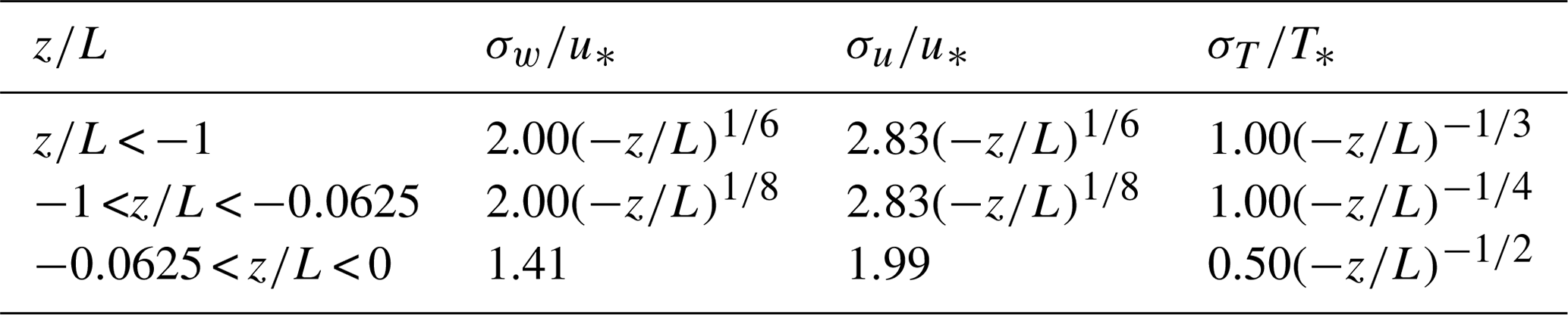
A second requirement for EC that is often used as a quality check is the test for developed turbulent conditions, as described by Foken and Wichura (1996). It is based on flux–variance similarity and makes use of the integral turbulence characteristics of atmospheric turbulence, which depend on stability:
where σx is the standard deviation of a fluctuating parameter x, X∗ is the corresponding dynamical parameter (e.g., σu and u∗ or σT and T∗), and the dimensionless height z∕L is the Monin–Obukhov stability parameter. Table 2 lists the coefficients c1 and c2 for w, u and T for different stability ranges as published by Foken et al. (1991, 1996). When does not differ by more than 50 % from the model, using the tabulated values for c1 and c2, developed turbulent conditions are considered to be fulfilled. It is noted that this test is location dependent, and the parameterization listed in Table 2 can deviate depending on local constraints. We tested the parameterization for Innsbruck and found that with published values for c1 and c2, which were not obtained over urban areas, the integral turbulence characteristics (ITC) test for commonly underestimates turbulent conditions over an urban area.
The flux detection limit is estimated by several different criteria.
Flux noise STD criterion (LoDσ). Here the values of the covariance function, Fc(τi), at unphysically large lag times, τi, are considered uncorrelated statistical noise (Wienhold et al., 1994; Spirig et al., 2005). Realizations of Fc(τi) are calculated for τi in intervals of [−180, −160 s] and [160, 180 s] with mF and σF describing the mean value and the standard deviation (STD) of Fc(τi). A covariance peak outside of the interval is considered significantly different from the flux noise and thus detectable.
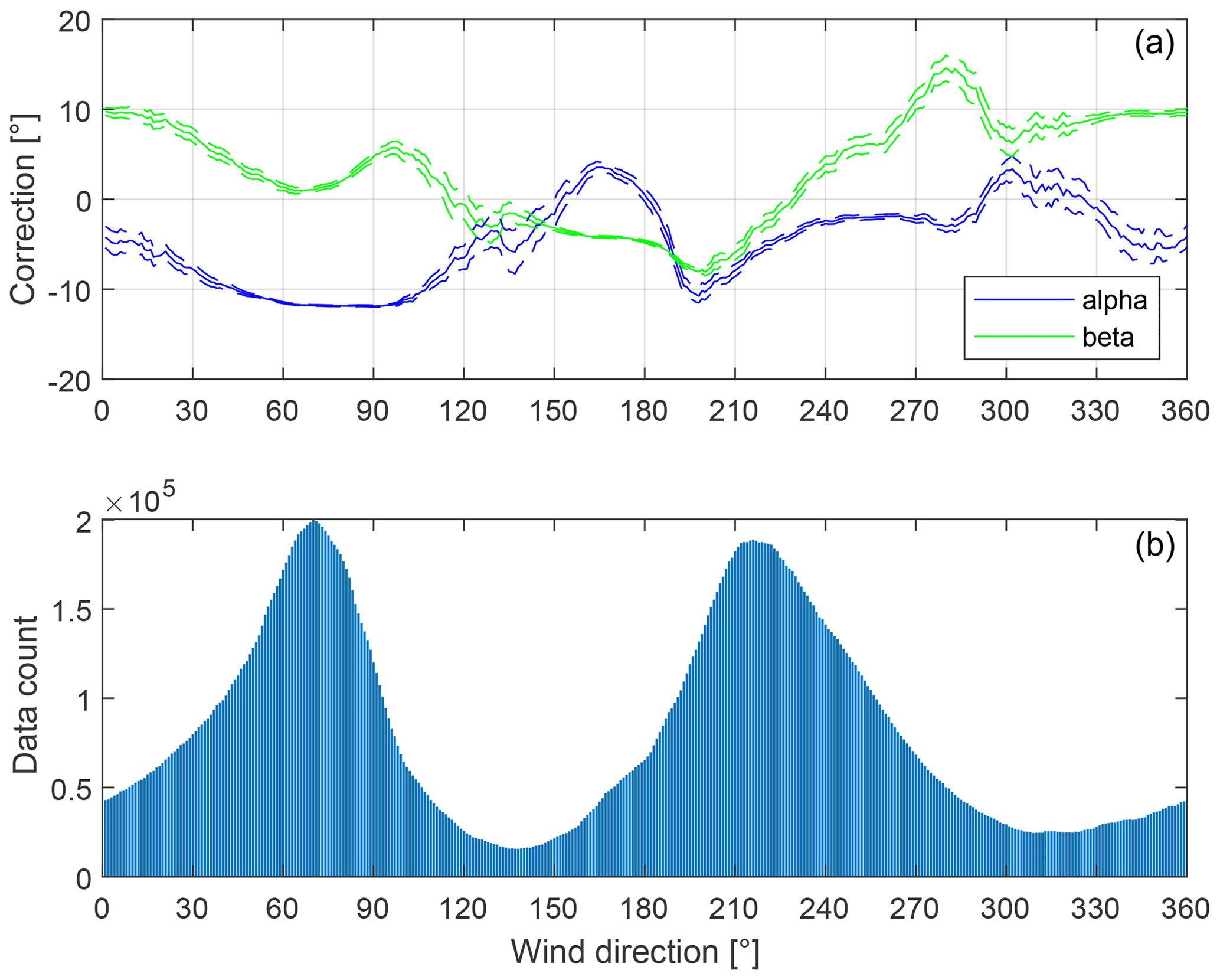
Figure 1(a) Sonic anemometer tilt correction angles dependent on the mean wind direction. For each mean wind direction, all available half-hour intervals of data with mean wind direction within ±15∘ were taken for determining the tilt correction angles according to the planar fit method. The dashed lines show 95 % confidence bounds estimated by bootstrapping. (b) The histogram shows the number of half-hour intervals contributing to the calculation of the correction angles.
Flux noise RMSE criterion (LoDRMSE). A modification of the previous approach was described by Langford et al. (2015), where instead of the standard deviation, the root of the mean squared deviation of Fc(τi) from 0 is calculated.
Random error criterion. Finkelstein and Sims (2001), described an approach based on variance of a covariance between two variables, which are first autocorrelated and cross-correlated:
“Random shuffle” method. Billesbach (2011) proposed another method for estimating the contribution of random instrument noise. Here one of the two variables (w′, c′) is randomly time-shuffled before recalculating the covariance, effectively removing the covariance due to turbulent transport mechanisms, leaving only the random correlations mostly attributable to instrument noise.
Autocovariance method. As described by Lenschow et al. (2000), Mauder et al. (2013) and Langford et al. (2015), instrumental noise of the covariance function is estimated by extrapolating the first four terms of the autocovariance function to zero lag and then taking the difference to its value at zero lag.
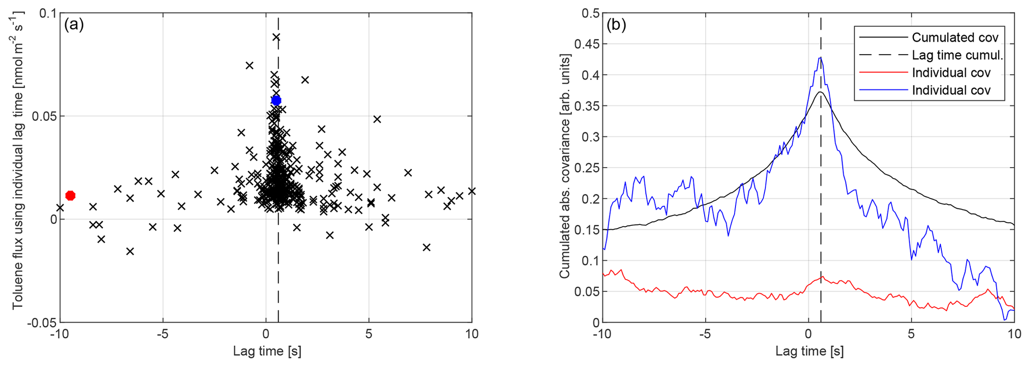
Figure 2(a) Lag time determined from individual averaging intervals dependent on the flux. For periods of small flux, individually determined lag time shows large scatter. (b) Individual and cumulated absolute cross-covariance function for toluene 13C isotope used for estimating the lag time. The dashed line shows the estimated lag time. The lag times corresponding to the individual covariance functions are shown as red and blue dots in the graph on the left.
Table 1Comparison of calculated fluxes using two different anemometer tilt correction methods with respect to no tilt correction. Slopes are determined by a robust linear fit through corrected data vs. uncorrected data and include 95 % confidence bounds.

Table 2Dependence of the integral turbulence characteristics for wind components w, u and temperature T on the stratification (Foken and Wichura, 1996; Foken et al., 1991).
3.1 Tilt correction
For the present urban dataset, sonic anemometer tilt correction angles were found to vary significantly with the direction of the mean wind. The observed variation is caused by the topography and the influence of surface roughness surrounding the urban measurement location, where tall buildings in the vicinity tend to deform the mean streamlines of the airflow from certain directions. For each mean wind direction, the mean wind vectors were therefore split into ±15∘ intervals to calculate a corresponding tilt correction matrix. The width of the interval is made large enough to have sufficient data for the planar fit method and small enough that the angle-dependent variation in the correction angles due to the topography is well resolved. Figure 1 shows the dependency of the sonic tilt correction angles on the mean wind direction, as well as the number of data points contributing to the determination of the tilt correction angles. The first rotation angle α is defined as the pitch angle about the original y axis, and the second rotation angle β is the roll angle measured about the new x axis.
Table 1 shows the impact of the two tilt correction methods on the resulting flux. Fluxes were calculated separately without tilt correction, with the double rotation method and with the planar fit method. The results were filtered by basic quality criteria, and the corrected data were plotted against the uncorrected data. A robust linear fit quantifies the impact of the tilt correction. Applying no tilt correction tends to overestimate the flux for the current dataset up to approximately 15 %.
3.2 The role of lag time determination
While lag time determination from a single averaging interval might prove to work well for times where the magnitude of the flux is sufficiently large, it will fail in many cases where the flux is small (e.g., close to detection limits). This behavior is illustrated in Fig. 2, where the individually determined lag times are plotted against the flux of toluene. For larger flux values the lag times show little variance, while for smaller fluxes the scatter increases significantly, thus for fluxes close to the detection limit conventional lag time determination fails, with most lag times outside a physically meaningful range. The data were chosen for a period of 34 d, when lag times were constant and variations due to changing instrumental conditions could be excluded. The dashed line marks the lag time determined from the cumulated absolute covariance functions over the same data range. Individually determined lag times for periods with large fluxes show little variability (±0.2 s) about this value. As toluene fluxes decrease, the variation in lag times becomes significant.
This finding suggests that a lag time from individual averaging intervals can only be determined reliably for periods of large flux (e.g., 3 times above LOD). During periods of small flux and signals just above the limit of detection, it will be very important to assure that the experimental setup produces results with small lag time variations so a cumulated covariance function can be used to obtain a reliable lag time. A Similar procedure was already described by Park et al. (2013). Our findings suggest that a cumulative lag time determination is preferable for fluxes that are close to or below the LOD of individual flux averaging intervals.
3.3 Comparison between eddy covariance and disjunct eddy covariance, including associated errors
For analytical instruments that do not allow us to simultaneously measure all chemical species of interest at once in a sequential manner, the disjunct eddy covariance (DEC) method can be applied. Alternatively, a physical disjunct sampler (Rinne et al., 2001; Warneke et al., 2002) can be used, when the measurement time requires longer integration times (e.g., up to 1 min). DEC results in a reduction of gross measurement time for each species, as the available measurement time is distributed between individual samples that are spaced apart by the DEC interval (e.g., 10 s). Therefore, the signal-to-noise ratio is reduced, which makes lag time determination more difficult and susceptive to statistical errors (see Sect. 3.2).
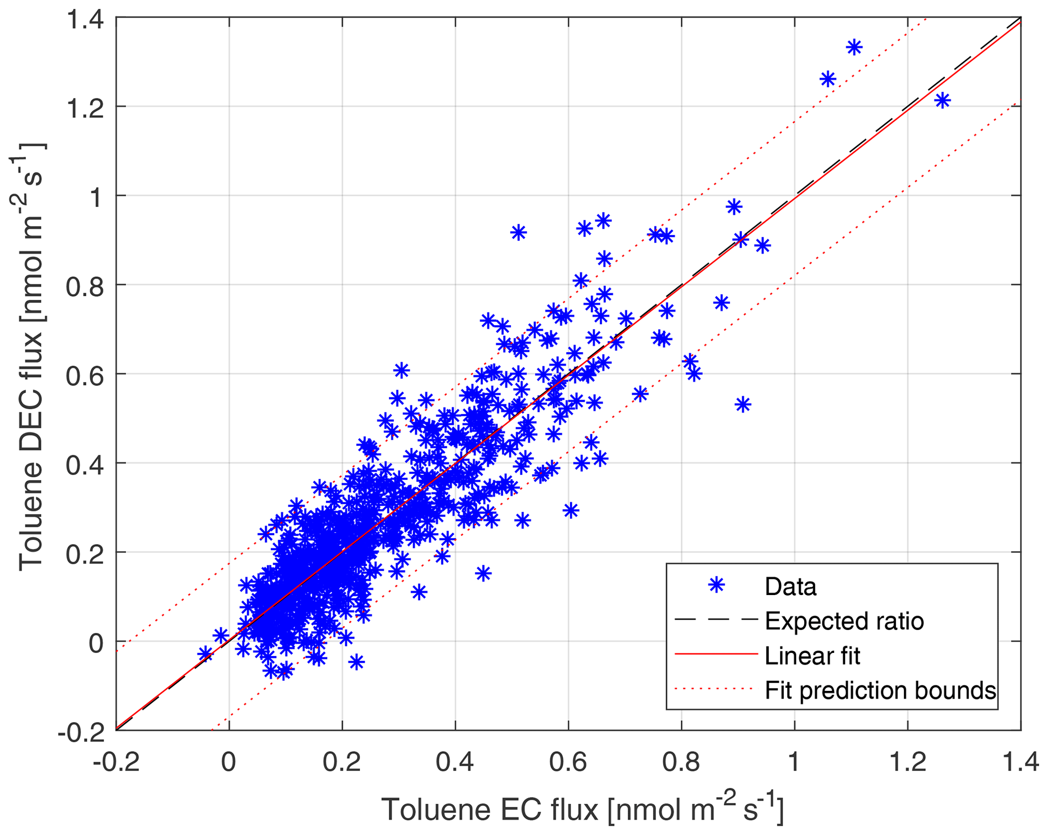
Figure 3Toluene flux determined by DEC (taking every 50th sample) vs. toluene flux determined by EC. The fitted curve shows very good correspondence between the DEC and EC flux results, with slope close to 1 (slope: 0.99; offset: 0.003; R2: 0.89).
To test the accuracy of lag time determination with disjunct EC data, artificial DEC datasets were created from a high-resolution EC dataset. Seven different DEC realizations were created by taking every 5th, 10th, 20th, 50th, 100th, 200th and 500th sample of the EC dataset, producing DEC datasets with disjunct sampling intervals between 0.5 and 50 s. As an example, Fig. 3 shows the DEC vs. the EC flux for toluene. As can be seen, the scatter around the 1:1 line is largely determined by increased statistical noise due to a smaller amount of data used for the DEC method (every 50th sample resulting in a DEC interval of 5 s). The slope is close to the 1:1 line, indicating that the systematic bias is small.
Systematic errors due to disjunct sampling can be assessed according to Lenschow et al. (1994), Eq. (55):
where T is the averaging interval, Δ is the sampling interval, F is the flux and τ is the integral timescale.
The random error can be estimated according to Lenschow et al. (1994), Eq. (58):
where μf is the variance of the time series with T→ ∞.
Figure 4 shows the relative systematic error for the artificial DEC dataset and the model curve according to Lenschow et al. Below the integral timescale τ (about 10 s) the systematic error is about 1 % and is mostly attributable to low-frequency loss due to the finite flux averaging period T of 1800 s. Above the integral timescale, the systematic error due to disjunct sampling starts to become significant and would amount to about a 15 % underestimation of the flux for a 300 s DEC interval. In general, we find that the influence of systematic errors is not the limiting constraint when measuring DEC fluxes, as long as DEC intervals are lower than about 1 min. Figure 5 shows the increase in the random error for the artificially created DEC dataset with increasing sampling interval and a fit of Lenschow's Eq. (58) to the data.
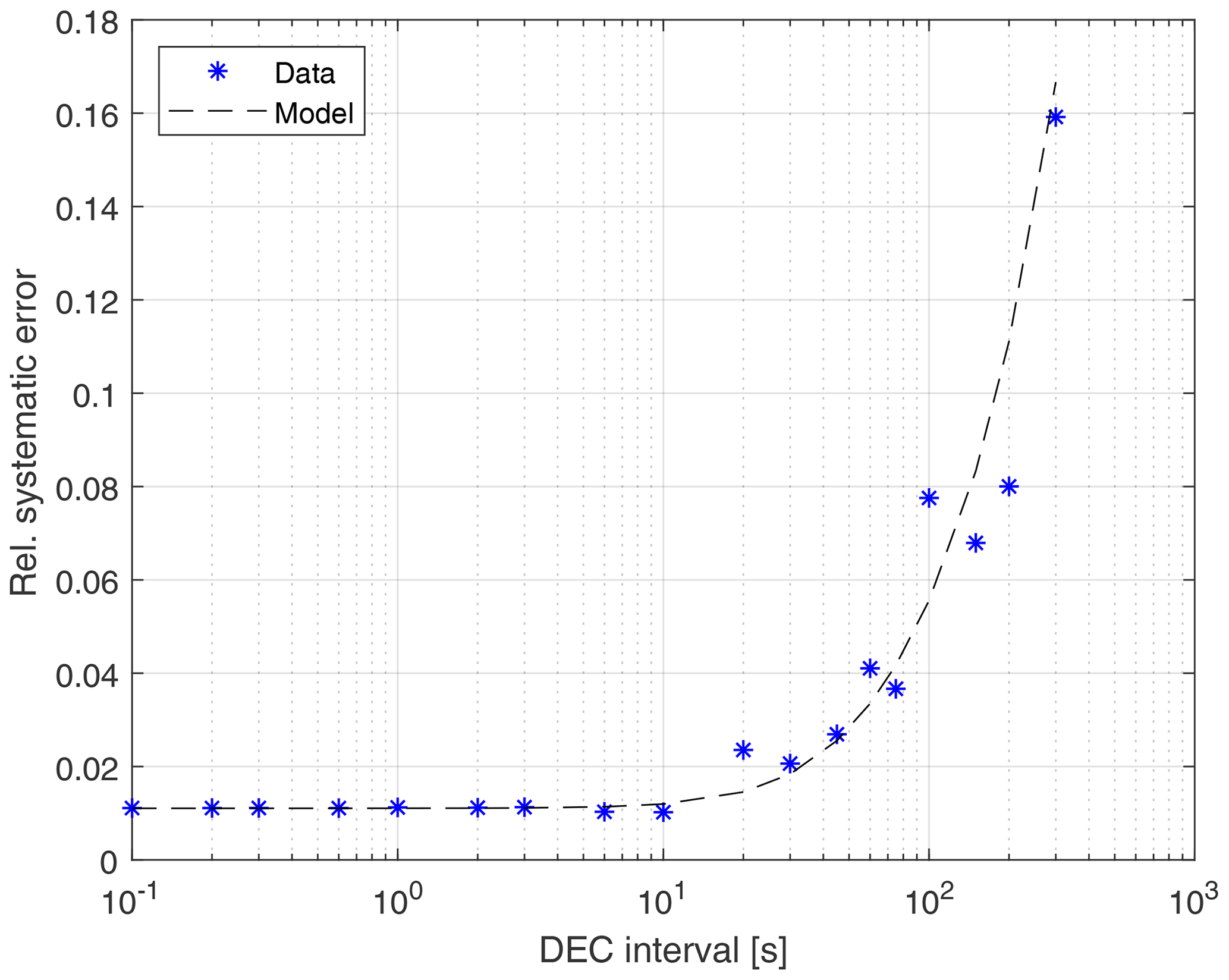
Figure 4Systematic error of toluene flux with increasing DEC sampling interval Δt determined by artificially created DEC datasets and according to Lenschow et al. (1994).
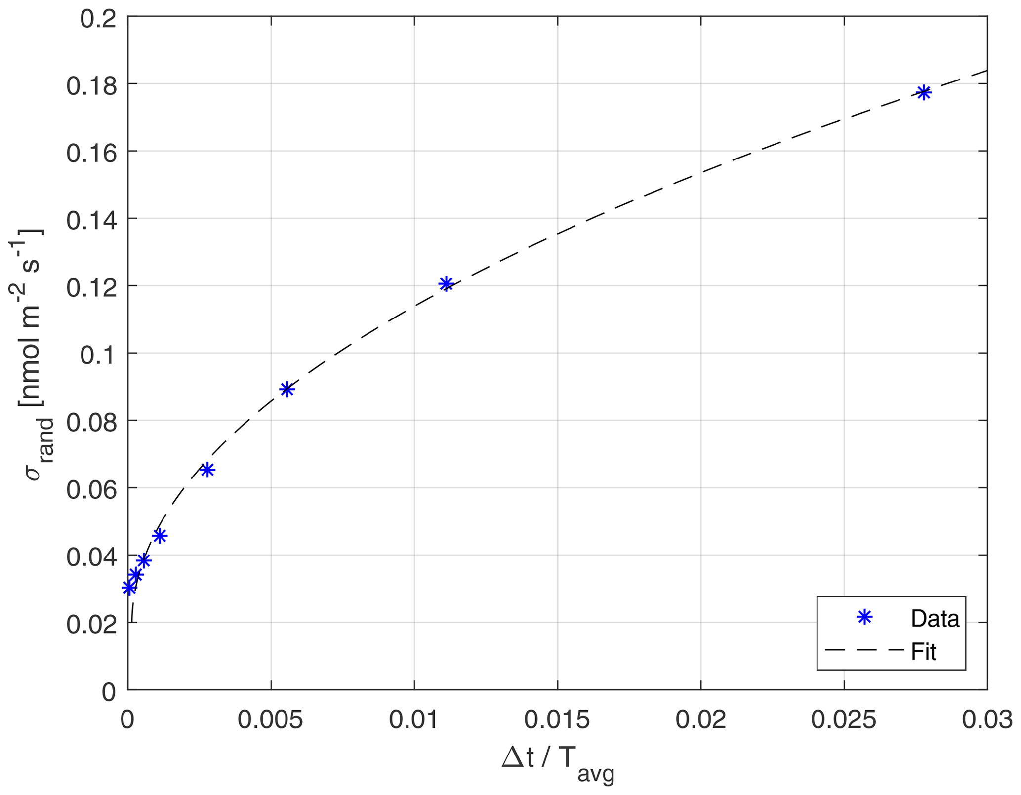
Figure 5Random error of toluene flux with increasing DEC sampling interval Δt determined by artificially created DEC datasets following a square-root relation.
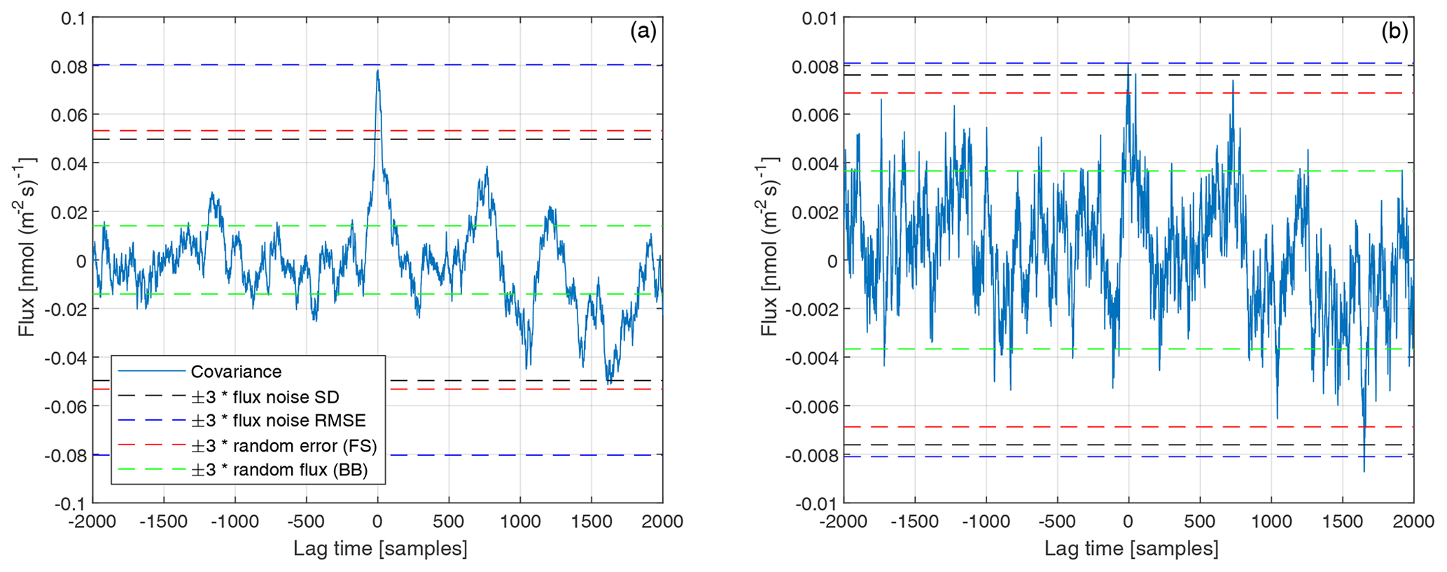
Figure 6Covariance function and limit of detection (LOD) for toluene (a) and its 13C isotope (b) estimated using different approaches.
3.4 Flux LOD
The flux limit of detection (LOD) for high and low signal-to-noise ratios estimated by four individual methods are plotted in Fig. 6. For practical reasons the first four methods described in Sect. 2.3.4 are implemented in the innFLUX code and are tested using an exemplary 30 min interval. As can be seen, the random flux method (Billesbach et al., 2011) likely underestimates the flux LOD, which could lead to erroneous flux LODs. The most conservative estimate for a flux LOD is obtained by the RMSE criterion (Langford et al., 2015). The criterion based on the random error (Finkelstein and Sims, 2001) or standard deviation of the covariance function (Wienhold et al., 1994; Spirig et al., 2005) lies between the other two methods.
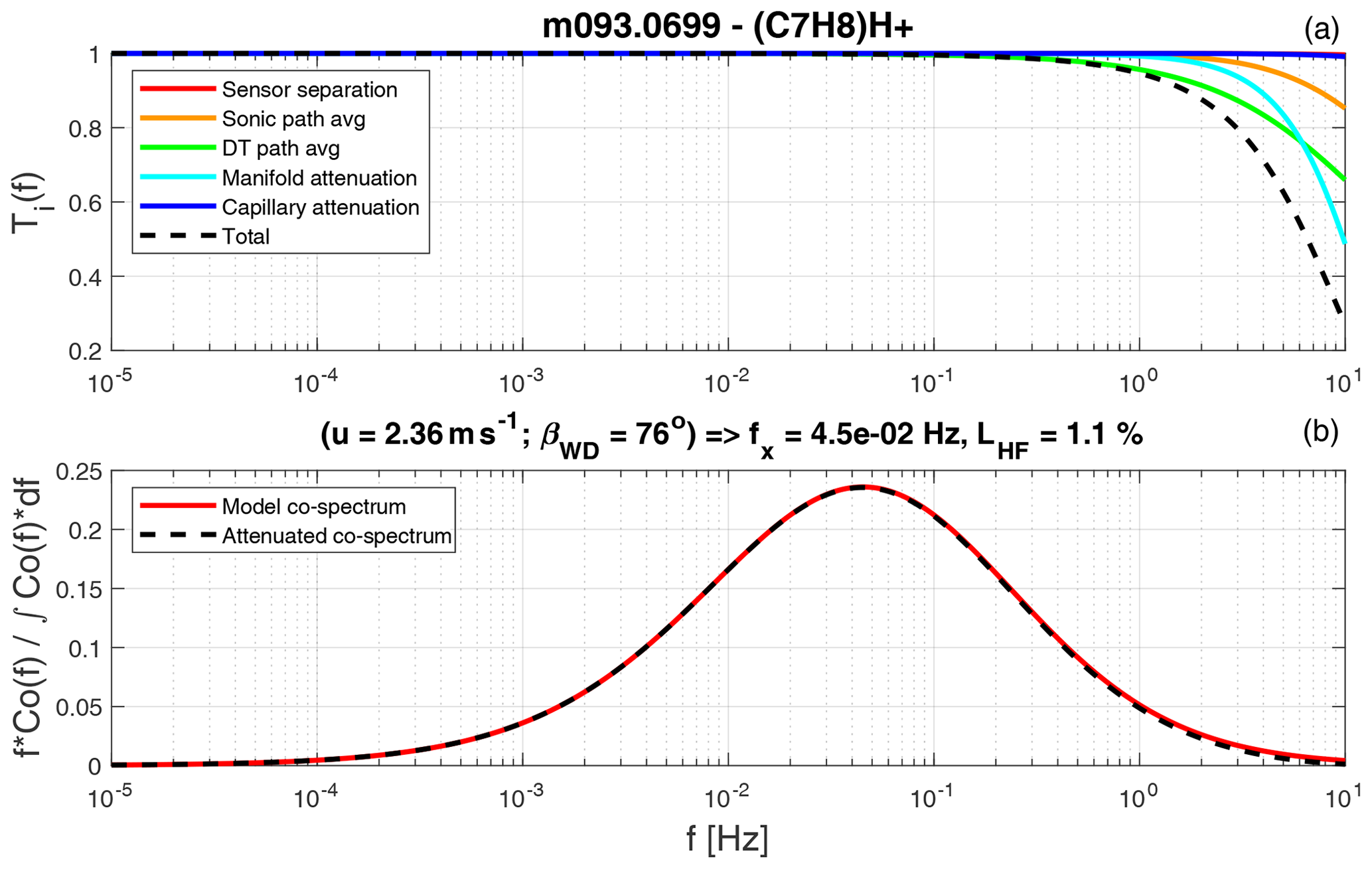
Figure 7Spectral analysis for toluene for the averaging period 11:30–12:00 UTC, 27 July 2015. Panel (a) shows individual transfer functions in color (see Sect. S4 in the Supplement for details) and the transfer function of the total high-frequency attenuation. Panel (b) shows the model co-spectrum (red) and the attenuated co-spectrum (black).
3.5 Spectral corrections
Co-spectral information calculated and stored by innFLUX (see Sect. 2.3.3) allow the user to correct measured eddy covariances for spectral attenuation. Two approaches to implement such corrections are suggested in the literature (see Foken et al., 2012, and the references therein): the so-called experimental approach assumes co-spectral similarity between the scalar to be corrected and some other quantity that shows no significant attenuation (e.g., sensible heat flux) in order to rescale the scalar that is subject to significant low-pass filtering. The theoretical approach requires the knowledge of a model co-spectrum appropriate to describe the “true” (i.e., unattenuated) co-spectral density of scalar and transfer functions for the processes that cause significant spectral losses. Which of the two approaches is better or whether there exists a meaningful way for spectral corrections at all cannot be decided without further consideration of the validity of the respective assumptions. Measurement station geometry and operational parameters, distribution of sources and roughness elements and the length and quality of the dataset must be taken into account for the user's decision whether and how to correct for co-spectral loss of covariance.
Exemplarily, here we detail the correction procedure for our urban test case. In such a setting, the sources of sensible heat flux (roofs and walls of buildings, ground surface, anthropogenic heat sources, etc.) are distributed quite differently from the sources of VOCs (e.g., vehicles with internal combustion engines emit toluene and these emissions are largely restricted to roads and heights close to the surface). This circumstance does not lend itself to the assumption of co-spectral similarity of the fluxes of sensible heat and VOCs. On the other hand, the dataset is sufficiently long to derive a model co-spectrum from stringently filtered individual co-spectra, and the operational and geometry parameters are well defined, thus allowing for the determination of transfer functions for the significant loss processes. Section S4 describes the determination of model co-spectra (see Fig. S4 in the Supplement) and the construction of the transfer function of the total high-frequency attenuation (Fig. 7a). Figure 7b shows the model spectrum (red) and the attenuated spectrum (black) of toluene for the averaging period 11:30–12:00 UTC, 27 July 2015. For this particular flux period the high-frequency loss was 1.1 %, and the mean loss for the 61 d dataset was 2 % (Sect. S4 and Fig. S5).
3.6 Comparison with established EC software
We processed our dataset with EddyPro®, a widely used eddy covariance processing software developed and maintained by LI-COR Inc., and we compared the results to those obtained by innFLUX. The results exhibit good agreement for trace gas fluxes and sensible heat flux. The details of that comparison are shown in the Supplement. Typical regression slopes show a slope of 1.02±0.009 and 0.954±0.006 for the CO2 flux and sensible heat flux, respectively.
We tested the applicability of disjunct eddy covariance and eddy covariance measurements in an urban air matrix using a newly designed software package in MATLAB. The code integrates our current understanding of how to deal with noisy data, which is an issue particularly for emerging high time resolution measurements of a wide range of NMVOCs, SVOCs and other trace gases that are becoming tractable based on highly sensitive time-of-flight mass spectrometry. We were able to test algorithms for finding cross-covariance peaks based on analyzing distinct isotopes (e.g., 12C and 13C toluene isotopes). Based on an extensive urban dataset, we evaluated realistic LODs for NMVOC flux measurements using a first-generation PTR-SRI-QiTOF-MS. For example, for toluene and benzene we found 5th–95th percentile LOD ranges of 0.025–0.19 and 0.047–0.49 nmol m−2 s−1, respectively. The high sensitivity allowed evaluating theoretical expressions of both random and systematic flux errors for NMVOCs due to undersampling. We observe an increase in systematic errors at DEC intervals of about 10 s. For DEC intervals of 300 s the systematic error amounts to 16 %. More importantly, the increase in random errors at such long disjunct time intervals becomes large, thus most NMVOC fluxes would likely fall below the observable flux LODs. The presented flux code and analysis also addresses potential sources of errors related to flux measurements above urban canopies. For example, we found that a directional tilt correction improved the accuracy of calculated fluxes by more than 10 % for most compounds.
The goal of this work was to develop, test and present a new software package for analyzing EC and DEC data of a wide range of species that are relevant for atmospheric chemistry and related disciplines. While we focused on the applicability for urban flux measurements in particular in this study, this software package is expected to be applicable in other environments that are not horizontally homogeneous.
The flux routine is written in MATLAB (tested with release R2018a). The input files need to be prepared as MATLAB data files as described in the section below.
If sonic tilt correction using the planar fit method is to be applied, a tilt correction file must be created first. This can be done by the innFLUX_step0 routine. Choose a dataset that is as large as possible and contains sonic data of a period during which the sonic anemometer was not moved. The routine will create a file “tilt_correction.mat”, which can be used as input in the following routine.
The actual flux routine is divided in two steps. The innFLUX_step1 routine calculates all meteorological data and the fluxes using the lag time determined from each single averaging interval. A file “results.mat” is created. The lag times in this file should be checked before proceeding with the second step of the flux routine. If the lag times scatter around the same mean value during the whole measurement period, no further action is required before proceeding with the next step. If the lag time shows sudden changes, the data range should be divided into several subranges, during which the lag time scatters around the same mean value. This is done by adjusting the data_segments parameter in the parameter file. The innFLUX_step2 routine calculates the lag times from covariances cumulated over the full data range or subranges of consistent lag times if data_segments are defined.
This section describes the format of the input data and the parameters in the parameter file.
All input files are MATLAB data files (.mat), unless otherwise stated.
B1 Parameter file
The parameter file is a MATLAB script file named “innFLUX_parameters.m” and contains path definitions and several parameters for configuring the flux routine. A template file “innFLUX_parameters_template.m” is provided to serve as a basis for the parameter file. For better distinction, arrays here are displayed with brackets, [], and cell arrays are displayed with braces, {}, which are not part of the variable name.
-
output_folder: folder where the output files will be stored
-
sonic_files_folders{}: one or more folders containing the sonic data files
-
tracer_files_folders{}: one or more folders containing the tracer files
-
tracer_files_prefix: filename prefix of the tracer files
-
tracer_files{}: one or more tracer files, only used if tracer_files_ folders{} is empty
-
tilt_correction_filepath: path of a tilt correction file created by the tilt correction routine (innFLUX_step0)
-
pressure_filepath: path of an optional file containing pressure data
-
irga_columns[]: column indices of IRGA data; leave empty if no IRGA data are present
-
irga_names{}: names of IRGA data; leave empty if no IRGA data are present
-
irga_H2O_index: determines which of the IRGA tracers is H2O; needed for temperature and WPL correction
-
irga_flag_column: column index of the IRGA data quality flag
-
tracer_indices[]: indices of tracers to be processed; if empty, all tracers are processed
-
data_segments[]: data segments, within which a common lag time is determined; if empty, the full data period is regarded as one single segment; format: vector of timestamps defining the borders of the segments, e.g., for two segments:
data_segments = [datenum(2019,7,1) datenum(2019,7,21) datenum(2019,8,7)];
-
SONIC_ORIENTATION: orientation of the sonic anemometer in degrees
-
SENSOR_HEIGHT: sensor height in meters above the roughness height
-
WINDOW_LENGTH: length of the averaging window in samples
-
SAMPLING_RATE_SONIC: sonic anemometer sampling rate in samples per second
-
SAMPLING_RATE_TRACER: trace gas analyzer sampling rate in samples per second
-
DISJUNCT_EC: if 1, disjunct eddy covariance is applied
-
DETREND_TEMPERATURE_SIGNAL: if 1, linear detrending is applied to temperature signal
-
DETREND_TRACER_SIGNAL: if 1, linear detrending is applied to tracer signals
-
MAX_LAG: maximum lag when calculating covariances in samples
-
LAG_SEARCH_RANGE: range (±) for lag time search in samples
-
COVPEAK_FILTER_LENGTH: smoothing length of filter applied to covariance function prior to finding the covariance peak in samples
-
NUM_FREQ_BINS: number of logarithmically spaced frequency bins for co-spectra
-
FREQ_BIN_MIN: lowest-frequency bin for scaled co-spectra
-
FREQ_BIN_MAX: highest-frequency bin for scaled co-spectra
-
TILT_CORRECTION_MODE: 0: no tilt correction; 1: double rotation; 2: directional planar fit
-
APPLY_WPL_CORRECTION: if 1, WPL correction is applied
-
COMPLETENESS_THRESHOLD: threshold value for completeness of input data, 0.0–1.0; below this threshold, results are not calculated and filled with NaN (not a number)
-
DEFAULT_PRESSURE: fixed pressure used if no pressure is given in the input files in hPa or mbar
-
SPIKE_DETECTION_THRESHOLD: standard deviations of the threshold for detecting spikes in the input data
-
SPIKE_DETECTION_WINDOW: samples of the width of the spike detection window
B2 Sonic data file format
Sonic files must contain exactly 1 d data each and be named “wyyyymmdd.mat”, where yyyy, mm and dd stand for the corresponding year, month and day, respectively, e.g., “w20190725.mat”. The routine can find all files following this naming convention inside one or more given folders. The sonic data files must contain the data of a full day each. Missing data should be filled with NaN (not a number) as a placeholder. Sonic files consist of a matrix, where the columns contain the following data.
-
Column 1: MATLAB timestamp;
-
Column 2: reserved;
-
Column 3: first horizontal component of the wind vector (in the sonic anemometer's coordinate system);
-
Column 4: second horizontal component of the wind vector;
-
Column 5: vertical component of the wind vector;
-
Column 6: sonic virtual temperature;
-
Column 7: sonic flag (this is normally 0, and it is different from 0 when there was an error in wind data acquisition);
-
Column 8..N (optional): concentration of a tracer measured by infrared gas analyzer (IRGA);
-
Column N+1 (optional): IRGA flag; (normally 0, and different from 0 when there was an error in IRGA data acquisition).
If one of the IRGA tracers is water vapor, the unit is expected to be per mil.
B3 Tracer data file format
The tracer data can be provided as files containing 1 d data each named with the prefix tracer_files_prefix as given in the parameter file followed by the corresponding day's date in the format “yyyymmdd.mat”, e.g., “ptrms20190725.mat”. The routine can find all files following this naming convention inside one or more given folders (tracer_files_folders).
Alternatively, the tracer data can be provided in one or more files of arbitrary name containing an arbitrarily large amount of data (tracer_files).
The tracer data files must consist of a structure containing the fields header and data. The header field is a cell array of strings containing the names of the columns in the data field. The first column in the data field contains the MATLAB timestamps, the other columns contain the tracer concentration data in ppb.
B4 Pressure data file format
Ambient pressure data can be provided in a separate MATLAB data file consisting of a struct containing the fields time and p. The field time must contain MATLAB timestamps, and the field p must contain the corresponding pressure data in hPa (mbar). Here pressure can be provided at lower sampling rates and is interpolated by the flux routine as needed.
Results file
The main output file is a MATLAB data file named “results.mat”. It consists of a struct containing the following fields:
-
time: timestamp of the beginning of each averaging interval in MATLAB time;
-
hour: hour of day;
-
freq: frequency axis of co-spectra in seconds;
-
freq_scaled: frequency axis of scaled co-spectra, , dimensionless;
-
MET.uvw: mean wind speed vector (u, v, w), with u pointing into the direction of mean wind in m s−1;
-
MET.std_uvw: standard deviation of wind speed components u, v and w in m s−1;
-
MET.hws: horizontal wind speed in m s−1;
-
MET.wdir: horizontal wind direction in degrees;
-
MET.tilt.P: tilt correction matrix applied to wind vectors;
-
MET.uw: covariance of along-wind and vertical wind component, < >, in m2 s−2;
-
MET.vw: covariance of crosswind and vertical wind component, < >, in m2 s−2;
-
MET.uv: covariance of along-wind and crosswind component, < >, in m2 s−2;
-
MET.uu: auto-covariance of along-wind component, < >, in m2 s−2;
-
MET.vv: auto-covariance of crosswind component, < >, in m2 s−2;
-
MET.ww: auto-covariance of vertical wind component, < >, in m2 s−2;
-
MET.ust: friction velocity, u*, in m s−1;
-
MET.T: temperature in Kelvin;
-
MET.std_T: standard deviation of mean temperature in Kelvin;
-
MET.wT: temperature flux, < >, in K m s−1;
-
MET.L: Obukhov length in meters;
-
MET.zoL: stability parameter, z∕L, dimensionless;
-
MET.cospec_wT: co-spectrum for wT, Co();
-
MET.cospec_wT_scaled: scaled co-spectrum for wT, f⋅Co() ∕ cov();
-
MET.p: pressure in hPa;
-
MET.theta: potential temperature in Kelvin;
-
MET.theta_v: virtual potential temperature in Kelvin;
-
MET.wtheta: potential temperature (heat) flux, < >, in K m s−1;
-
MET.wtheta_v: virtual potential temperature (buoyancy) flux, < >, in K m s−1;
-
MET.qaqc.completeness: fraction of sonic data used in this averaging interval;
-
MET.qaqc.SST_wT: relative deviation in steady-state test for wT;
-
MET.qaqc.ITC_w: relative model deviation of integral turbulence characteristics test for w;
-
MET.qaqc.ITC_u: relative model deviation of integral turbulence characteristics test for u;
-
MET.qaqc.ITC_T: relative model deviation of integral turbulence characteristics test for T;
-
MET.qaqc.cospec_wT_integral: integral of co-spectrum for wT;
-
IRGA(i).name: name of ith tracer measured by IRGA;
-
IRGA(i).mean: mean concentration;
-
IRGA(i).std: standard deviation of concentration;
-
IRGA(i).lagtime1: lag time determined individually for this averaging interval in seconds;
-
IRGA(i).flux1: flux calculated using lagtime1 in nmol m−2 s−1 if tracer concentration is given in ppbv;
-
IRGA(i).lagtime2: lag time determined from cumulated covariance functions in seconds;
-
IRGA(i).flux2: flux calculated using lagtime2 in nmol m−2 s−1 if tracer concentration is given in ppbv;
-
IRGA(i).cospec: co-spectrum for w and tracer concentration, Co();
-
IRGA(i).cospec_scaled: scaled co-spectrum for w and tracer concentration, f⋅ Co() ∕ cov();
-
IRGA(i).qaqc.completeness: fraction of tracer data used in this interval;
-
IRGA(i).qaqc.SST: relative deviation in steady-state test for tracer;
-
IRGA(i).qaqc.flux_SNR: flux signal-to-noise ratio;
-
IRGA(i).qaqc.flux_noise_std: standard deviation of flux noise that is far off the integral timescale;
-
IRGA(i).qaqc.flux_noise_mean: mean flux noise far off the integral timescale;
-
IRGA(i).qaqc.flux_noise_rmse: RMSE of flux noise far off the integral timescale;
-
IRGA(i).qaqc.random_error_FS: random error as described by Finkelstein and Sims (2001);
-
IRGA(i).qaqc.random_error_noise: random error noise estimated according to Mauder (2013);
-
IRGA(i).qaqc.random_flux: random flux level estimated by random shuffle criteria (Billesbach, 2011);
-
IRGA(i).qaqc.cospec_integral: integral of co-spectrum;
-
TRACER(i).name: name of ith tracer;
-
TRACER(i).mean: mean concentration in ppb;
-
TRACER(i).std: standard deviation of (detrended) tracer concentration in ppb;
-
TRACER(i).lagtime1: lag time determined individually for this averaging interval in seconds;
-
TRACER(i).flux1: flux calculated using lagtime1 in nmol m−2 s−1;
-
TRACER(i).lagtime2: lag time determined from cumulated covariance functions in seconds;
-
TRACER(i).flux2: flux calculated using lagtime2 in nmol m−2 s−1;
-
TRACER(i).wpl_corr: WPL correction term in nmol m−2 s−1;
-
TRACER(i).cospec: co-spectrum for w and tracer concentration, Co();
-
TRACER(i).cospec_scaled: scaled co-spectrum for w and tracer concentration, f⋅ Co() ∕ cov();
-
TRACER(i).qaqc.completeness: fraction of tracer data used in this interval;
-
TRACER(i).qaqc.SST: relative deviation in steady-state test for tracer
-
TRACER(i).qaqc.flux_SNR: flux signal-to-noise ratio;
-
TRACER(i).qaqc.flux_noise_std: standard deviation of flux noise far off the integral timescale;
-
TRACER(i).qaqc.flux_noise_mean: mean flux noise far off the integral timescale;
-
TRACER(i).qaqc.flux_noise_rmse: RMSE of flux noise far off the integral timescale;
-
TRACER(i).qaqc.random_error_FS: random error as described by Finkelstein and Sims (2001);
-
TRACER(i).qaqc.random_error_noise: random error noise estimated according to Mauder (2013);
-
TRACER(i).qaqc.random_flux: random flux level estimated by random shuffle criteria (Billesbach, 2011);
-
TRACER(i).qaqc.cospec_integral: integral of co-spectrum.
The code, along with a test dataset, can be downloaded from the website of the University of Innsbruck Atmospheric Physics and Chemistry (APC) group: https://www.atm-phys-chem.at/innflux (Karl, 2020).
The supplement related to this article is available online at: https://doi.org/10.5194/amt-13-1447-2020-supplement.
MS, MG and TGK conceived the data analysis codes and study. MG and MS conducted the measurements for the study. MS, MG and TGK analyzed the data, interpreted the results and wrote the paper. TDM contributed to editing the manuscript.
The authors declare that they have no conflict of interest.
This research has been supported by the Austrian Science Fund (FWF) (grant no. P 30600).
This paper was edited by Eric C. Apel and reviewed by Janne Rinne and Erik Velasco.
Aubinet, M., Vesala, T, and Papale, D.: Eddy Covariance: A Practical Guide to Measurement and Data Analysis, Springer Atmospheric Sciences, ISBN 978-94-007-2350-4, https://doi.org/10.1007/978-94-007-2351-1, 2012.
Ammann, C., Wolff, V., Marx, O., Brümmer, C., and Neftel, A.: Measuring the biosphere-atmosphere exchange of total reactive nitrogen by eddy covariance, Biogeosciences, 9, 4247–4261, https://doi.org/10.5194/bg-9-4247-2012, 2012.
Baldocchi, D. D., Hicks, B. B., and Meyers, T. P.: Measuring biosphere-atmosphere exchanges of biologically related gases with micrometeorological methods, Ecology, 69, 1331–1340, https://doi.org/10.2307/1941631, 1988.
Billesbach, D. P.: Estimating uncertainties in individual eddy covariance flux measurements: A comparison of methods and a proposed new method, Agr. Forest Meteorol., 151, 394–405, https://doi.org/10.1016/j.agrformet.2010.12.001, 2011.
Blomquist, B. W., Huebert, B. J., Fairall, C. W., and Faloona, I. C.: Determining the sea-air flux of dimethylsulfide by eddy correlation using mass spectrometry, Atmos. Meas. Tech., 3, 1–20, https://doi.org/10.5194/amt-3-1-2010, 2010.
Cooper, W. A. and Shertz, S.: An intermittent-sampling system for measuring fluxes from aircraft, in: Preprints, Ninth Symp. on Meteorological Observations and Instrumentation, Charlotte, NC, Amer. Meteor. Soc., 189–194, 1995.
Christen, A.: Atmospheric measurement techniques to quantify greenhouse gas emissions from cities, Urban Climate, 10, 241–260, https://doi.org/10.1016/j.uclim.2014.04.006, 2014.
Dabberdt, W. F., Lenschow, D. H., Horst, T. W., Zimmerman, P. R., Oncley, S. P., and Delany, A. C.: Atmosphere-surface exchange measurements, Science, 260, 1472–1481, https://doi.org/10.1126/science.260.5113.1472, 1993.
DeCarlo, P. F., Kimmel, J. R., Trimborn, A., Northway, M. J., Jayne, J. T., Aiken, A. C., Gonin, M., Fuhrer, K., Horvath, T., Docherty, K. S., Worsnop, D. R., and Jimenez, J. L.: Field-Deployable, high-resolution, time-of-flight aerosol mass spectrometer, Anal. Chem., 78, 8281–8289, https://doi.org/10.1021/ac061249n, 2006.
De Gouw, J., Warneke, C., Karl, T. G., Eerdekens, G., Van der Veen, C., and Fall, R.: Sensitivity and specificity of atmospheric trace gas detection by proton-transfer-reaction mass spectrometry, IJMS, 223–224, 365–382, https://doi.org/10.1016/S1387-3806(02)00926-0, 2003.
Deventer, M. J., Held, A., El-Madany, T. S., and Klemm, O.: Size-resolved eddy covariance fluxes of nucleation to accumulation mode aerosol particles over a coniferous forest, Agr. Forest Meteorol., 214–215, 328–340, https://doi.org/10.1016/j.agrformet.2015.08.261, 2015.
DiGangi, J. P., Boyle, E. S., Karl, T., Harley, P., Turnipseed, A., Kim, S., Cantrell, C., Maudlin III, R. L., Zheng, W., Flocke, F., Hall, S. R., Ullmann, K., Nakashima, Y., Paul, J. B., Wolfe, G. M., Desai, A. R., Kajii, Y., Guenther, A., and Keutsch, F. N.: First direct measurements of formaldehyde flux via eddy covariance: implications for missing in-canopy formaldehyde sources, Atmos. Chem. Phys., 11, 10565–10578, https://doi.org/10.5194/acp-11-10565-2011, 2011.
Ducker, J. A., Holmes, C. D., Keenan, T. F., Fares, S., Goldstein, A. H., Mammarella, I., Munger, J. W., and Schnell, J.: Synthetic ozone deposition and stomatal uptake at flux tower sites, Biogeosciences, 15, 5395–5413, https://doi.org/10.5194/bg-15-5395-2018, 2018.
Farmer, D. K., Chen, Q., Kimmel, J. R., Docherty, K. S., Nemitz, E., Artaxo, P. A., Cappa, C. D., Martin, S. T., and Jimenez, J. L.: Chemically Resolved Particle Fluxes Over Tropical and Temperate Forests, Aerosol Sci. Tech., 47, 818–830, https://doi.org/10.1080/02786826.2013.791022, 2013.
Finkelstein, P. L. and Sims, P. F.: Sampling error in eddy correlation flux measurements, J. Geophys. Res., 106, 3503–3509, https://doi.org/10.1029/2000JD900731, 2001.
Foken, T. and Wichura, B.: Tools for quality assessment of surface-based flux measurements, Agr. Forest Meteorol., 78, 83–105, https://doi.org/10.1016/0168-1923(95)02248-1, 1996.
Foken, T., Skeib, G. and Richter, S. H.: Dependence of the integral turbulence characteristics on the stability of stratification and their use for Doppler-Sodar measurements, Z. Meteorol., 41, 311–315, 1991.
Foken, T, Leuning, R., Oncley, S. R., Mauder, M., and Aubinet, M.: Corrections and Data Quality Control, in: Eddy Covariance: A Practical Guide to Measurement and Data Analysis, edited by: Aubinet, M., Vesala, T., and Papale, D., Dordrecht: Springer Netherlands, https://doi.org/10.1007/978-94-007-2351-1_4, 2012.
Fowler, D., Pilegaard, K., Sutton, M. A., Ambus, P., Raivonen, M., Duyzer, J., Simpson, D., Fagerli, H., Fuzzi, S., Schjoerring, J. K., Granier, C., Neftel, A., Isaksen, I. S. A., Laj, P., Maione, M., Monks, P.S., Burkhardt, J., Daemmgen, U., Neirynck, J., Personne, E., Wichink-Kruit, R., Butterbach-Bahl, K., Flechard, C., Tuovinen, J. P., Coyle, M., Gerosa, G., Loubet, B., Altimir, N., Gruenhage, L., Ammann, C., Cieslik, S., Paoletti, E., Mikkelsen, T. N., Ro-Poulsen, H., Cellier, P., Cape, J. N., Horvath, L., Loreto, F., Niinemets, Ü., Palmer, P. I., Rinne, J., Misztal, P., Nemitz, E., Nilsson, D., Pryor, S. C., Gallagher, M. W., Vesala, T., Skiba, U., Brüggemann, N., Zechmeister-Boltenstern, S., Williams, J., O'Dowd, C., Facchini, M. C., de Leeuw, G., Flossman, A., Chaumerliac, N., and Erisman, J. W.: Atmospheric composition change: Ecosystems–Atmosphere interactions, Atmos. Environ., 43, 5193–5267, https://doi.org/10.1016/j.atmosenv.2009.07.068, 2009.
Fratini, G. and Mauder, M.: Towards a consistent eddy-covariance processing: an intercomparison of EddyPro and TK3, Atmos. Meas. Tech., 7, 2273–2281, https://doi.org/10.5194/amt-7-2273-2014, 2014.
Graus, M., Müller, M., and Hansel, A.: High resolution PTR-TOF: Quantification and formula confirmation of VOC in real time, J. Am. Soc. Mass Spectrom., 21, 1037–1044, https://doi.org/10.1016/j.jasms.2010.02.006, 2010.
Guenther, A. and Hills, A.: Eddy covariance measurement of isoprene fluxes, J. Geophys. Res., 103, 13145–13152, https://doi.org/10.1029/97JD03283, 1998.
Hansel, A., Jordan, A., Holzinger, R., Prazeller, P., Vogel, W., and Lindinger, W.: Proton transfer reaction mass spectrometry: on-line trace gas analysis at the ppb level, Int. J. Mass Spectrom., 149/150, 609–619, https://doi.org/10.1016/0168-1176(95)04294-U, 1995.
Held, A., Niessner, R., Bosveld, F., Wrzesinsky, T., and Klemm, O.: Evaluation and application of an electrical low pressure impactor in disjunct eddy covariance aerosol flux measurements, Aerosol Sci. Tech., 41, 510–519, https://doi.org/10.1080/02786820701227719, 2007.
Horst, T. W., Kleissl, J., Lenschow, D. H., Meneveau, C., Moeng, C.-H., Parlange, M. B., Sullivan, P. P., and Weil, J. C.: HATS: Field observations to obtain spatially filtered turbulence fields from crosswind Arrays of sonic anemometers in the atmospheric surface layer, J. Atmos. Sci., 61, 1566–1581, https://doi.org/10.1175/1520-0469(2004)061<1566:HFOTOS>2.0.CO;2, 2004.
Hörtnagl, L., Clement, R., Graus, M., Hammerle, A., Hansel, A., and Wohlfahrt, G.: Dealing with disjunct concentration measurements in eddy covariance applications: a comparison of available approaches, Atmos. Env., 44, 2024–2032, https://doi.org/10.1016/j.atmosenv.2010.02.042, 2010.
Jordan, A., Haidacher, S., Hanel, G., Hartungen, E., Märk, L., Seehauser, H., Schottkowsky, R., Sulzer, P., and Märk, T. D.: A high resolution and high sensitivity proton-transfer-reaction time-of-flight mass spectrometer (PTR-TOF-MS), IJMS, 286, 122–128, https://doi.org/10.1016/j.ijms.2009.07.005, 2009.
Karl, T., Guenther A., Lindinger C., Jordan A., Fall R., and Lindinger, W.: Eddy covariance measurements of oxygenated volatile organic compound fluxes from crop harvesting using a redesigned proton-transfer-reaction mass spectrometer, J. Geophys. Res., 106, 24157–24167, https://doi.org/10.1029/2000JD000112, 2001.
Karl, T., Harley, P., Emmons, L., Thornton, B., Guenther, A., Basu, C., Turnipseed, A., and Jardine, K.: Efficient atmospheric cleansing of oxidized organic trace gases by vegetation, Science, 330, 816–819, https://doi.org/10.1126/science.1192534, 2010.
Karl, T., Misztal, P. K., Jonsson, H. H., Shertz, S., Goldstein, A. H., and Guenther, A. B.: Airborne flux measurements of BVOCs above Californian oak forests: Experimental investigation of surface and entrainment fluxes, OH densities and Dahmkoehler numbers, J. Atmos. Sci., 70, 3277–3287, https://doi.org/10.1175/JAS-D-13-054.1, 2013.
Karl, T., Striednig, M., Graus, M., Hammerle, A., and Wohlfahrt, G.: Urban flux measurements reveal a large pool of oxygenated volatile organic compound emissions, P. Natl. Acad. Sci., 115, 1186–1191, https://doi.org/10.1073/pnas.1714715115, 2018.
Karl, T. G.: InnFLUX webpage of the Atmospheric Physics and Chemistry Group, ACINN, University of Innsbruck, available at: https://www.atm-phys-chem.at/innflux, last access: 22 March 2020.
Karl, T. G., Spirig, C., Rinne, J., Stroud, C., Prevost, P., Greenberg, J., Fall, R., and Guenther, A.: Virtual disjunct eddy covariance measurements of organic compound fluxes from a subalpine forest using proton transfer reaction mass spectrometry, Atmos. Chem. Phys., 2, 279–291, https://doi.org/10.5194/acp-2-279-2002, 2002.
Kaser, L., Karl, T., Guenther, A., Graus, M., Schnitzhofer, R., Turnipseed, A., Fischer, L., Harley, P., Madronich, M., Gochis, D., Keutsch, F. N., and Hansel, A.: Undisturbed and disturbed above canopy ponderosa pine emissions: PTR-TOF-MS measurements and MEGAN 2.1 model results, Atmos. Chem. Phys., 13, 11935–11947, https://doi.org/10.5194/acp-13-11935-2013, 2013.
Kroon, P. S., Hensen, A., Jonker, H. J. J., Zahniser, M. S., van 't Veen, W. H., and Vermeulen, A. T.: Suitability of quantum cascade laser spectroscopy for CH4 and N2O eddy covariance flux measurements, Biogeosciences, 4, 715–728, https://doi.org/10.5194/bg-4-715-2007, 2007.
Langford, B., Davison, B., Nemitz, E., and Hewitt, C. N.: Mixing ratios and eddy covariance flux measurements of volatile organic compounds from an urban canopy (Manchester, UK), Atmos. Chem. Phys., 9, 1971–1987, https://doi.org/10.5194/acp-9-1971-2009, 2009.
Langford, B., Nemitz, E., House, E., Phillips, G. J., Famulari, D., Davison, B., Hopkins, J. R., Lewis, A. C., and Hewitt, C. N.: Fluxes and concentrations of volatile organic compounds above central London, UK, Atmos. Chem. Phys., 10, 627–645, https://doi.org/10.5194/acp-10-627-2010, 2010.
Langford, B., Acton, W., Ammann, C., Valach, A., and Nemitz, E.: Eddy-covariance data with low signal-to-noise ratio: time-lag determination, uncertainties and limit of detection, Atmos. Meas. Tech., 8, 4197–4213, https://doi.org/10.5194/amt-8-4197-2015, 2015.
Lenschow, D.H. and Kristensen, L.: Uncorrelated noise in turbulence measurements, J. Atmos. Ocean. Tech. 2, 68–81, https://doi.org/10.1175/1520-0426(1985)002<0068:UNITM>2.0.CO;2, 1985.
Lenschow, D. H., Mann, J., and Kristensen, L.: How long is long enough when measuring fluxes and other turbulence statistics?, J. Atmos. Ocean. Tech., 11, 661–673, https://doi.org/10.1175/1520-0426(1994)011<0661:HLILEW>2.0.CO;2, 1994.
Lenschow, D. H., Wulfmeyer, V., and Senff, C.: Measuring second through fourth-order moments in noisy data, J. Atmos. Ocean. Tech., 17, 1330–1347, https://doi.org/10.1175/1520-0426(2000)017<1330:MSTFOM>2.0.CO;2, 2000.
Mauder, M., Foken, T., Clement, R., Elbers, J. A., Eugster, W., Grünwald, T., Heusinkveld, B., and Kolle, O.: Quality control of CarboEurope flux data – Part 2: Inter-comparison of eddy-covariance software, Biogeosciences, 5, 451–462, https://doi.org/10.5194/bg-5-451-2008, 2008.
Mauder, M., Cuntz, M., Druee, C., Graf, A., Rebmann, C., Schmid, H. P., Schmidt, M., and Steinbrecher, R.: A strategy for quality and uncertainty assessment of long-term eddy-covariance measurements, Agr. Forest Meteorol., 169, 122–135, https://doi.org/10.1016/j.agrformet.2012.09.006, 2013.
Massman, W. J. and Clement, R.: Uncertainty in eddy covariance flux estimates resulting from spectral attenuation, in: Handbook of Micrometeorology: A Guide to Surface Flux Measurements, edited by: Lee, X., Massman, W., and Law, B., Springer Science + Business Media, Inc., 67–99, ISBN 978-1-4020-2265-4, https://doi.org/10.1007/1-4020-2265-4, 2004.
McDonald, B. C., de Gouw, J. A., Gilman, J. B., Jathar, S. H., Akherati, A., Cappa, C. D., Jimenez, J. L., Lee-Taylor, J., Hayes, P. L., McKeen, S. A., Cui, Y. Y., Kim, S-W., Gentner, D. R., Isaacman-VanWertz, G., Goldstein, A. H., Harley, R. A., Frost, G. J., Roberts, J. M., Ryerson, T. B., and Trainer, M.: Volatile chemical products emerging as largest petrochemical source of urban organic emissions, Science 359, 760–764, https://doi.org/10.1126/science.aaq0524, 2018.
Metzger, S., Durden, D., Sturtevant, C., Luo, H., Pingintha-Durden, N., Sachs, T., Serafimovich, A., Hartmann, J., Li, J., Xu, K., and Desai, A. R.: eddy4R 0.2.0: a DevOps model for community-extensible processing and analysis of eddy-covariance data based on R, Git, Docker, and HDF5, Geosci. Model Dev., 10, 3189–3206, https://doi.org/10.5194/gmd-10-3189-2017, 2017.
Moncrieff, J., Clement, R., Finnigan, J., and Meyers, T.: Averaging, detrending, and filtering of eddy covariance time series, in: Handbook of Micrometeorology: A Guide to Surface Flux Measurements, edited by: Lee, X., Massman, W., and Law, B., Springer Science + Business Media, Inc., 67–99, ISBN 978-1-4020-2265-4, https://doi.org/10.1007/1-4020-2265-4, 2004.
Muller, J. B. A., Coyle, M., Fowler, D., Gallagher, M. W., Nemitz, E. G., and Percival, C. J.: Comparison of ozone fluxes over grassland by gradient and eddy covariance technique, Atmos. Sci. Lett., 10, 164–169, https://doi.org/10.1002/asl.226, 2009.
Müller, M., Graus, M., Ruuskanen, T. M., Schnitzhofer, R., Bamberger, I., Kaser, L., Titzmann, T., Hörtnagl, L., Wohlfahrt, G., Karl, T., and Hansel, A.: First eddy covariance flux measurements by PTR-TOF, Atmos. Meas. Tech., 3, 387–395, https://doi.org/10.5194/amt-3-387-2010, 2010.
Nemitz, E., Jimenez, J. L., Huffman, J. A., Ulbrich, I. M., Canagaratna, M. R., Worsnop, D. R., and Guenther, A. B.: An eddy-covariance system for the measurement of surface/atmosphere exchange fluxes of submicron aerosol chemical species – First application above an urban area, Aerosol Sci. Tech., 42, 636–657, https://doi.org/10.1080/02786820802227352, 2008.
Nguyen, T. B., Crounse, J. D., Teng, A. P., St. Clair, J. M., Paulot, F., Wolfe, G. M., and Wennberg, P. O.: Rapid deposition of oxidized biogenic compounds to a temperate forest, P. Natl. Acad. Sci. USA, 112, E392–E401, https://doi.org/10.1073/pnas.1418702112, 2015.
Oncley, S. P., Foken, T., Vogt, R., Kohsiek, W., DeBruin, H. A. R., Bernhofer, C., Christen, A., van Gorsel, E., Grantz, D., Feigenwinter, C., Lehner, I., Liebethal, C., Liu, H., Mauder, M., Pitacco, A., Ribeiro, L., and Weidinger, T.: The Energy Balance Experiment EBEX-2000. Part I: overview and energy balance, Bound.-Lay. Meteorol. 123, 1–28, https://doi.org/10.1007/s10546-007-9161-1, 2007.
Park, J.-H., Goldstein, A. H., Timkovsky, J., Fares, S., Weber, R., Karlik, J., and Holzinger, R.: Active atmosphere-ecosystem exchange of the vast majority of detected volatile organic compounds, Science, 341, 643–647, https://doi.org/10.1126/science.1235053, 2013.
Patton, E. G., Horst, T. W., Sullivan, P. P., Lenschow, D. H., Oncley, S. P., Brown, W. O. J., Burns, S. P., Guenther, A. B., Held, A., Karl, T., Mayor, S. D., Rizzo, L. V., Spuler, S. M., Sun, J., Turnipseed, A. A., Allwine, E. J., Edburg, S. L., Lamb, B. K., Avissar, R., Calhoun, R. J., Kleissl, J., Massman, W. J., Paw U, K. T., and Weil, J. C.: The Canopy Horizontal Array Turbulence Study (CHATS), B. Am. Meteorol. Soc., 92, 593–611, https://doi.org/10.1175/2010bams2614.1, 2011.
Rannik, Ü., Altimir, N., Mammarella, I., Bäck, J., Rinne, J., Ruuskanen, T. M., Hari, P., Vesala, T., and Kulmala, M.: Ozone deposition into a boreal forest over a decade of observations: evaluating deposition partitioning and driving variables, Atmos. Chem. Phys., 12, 12165–12182, https://doi.org/10.5194/acp-12-12165-2012, 2012.
Rantala, P., Järvi, L., Taipale, R., Laurila, T. K., Patokoski, J., Kajos, M. K., Kurppa, M., Haapanala, S., Siivola, E., Petäjä, T., Ruuskanen, T. M., and Rinne, J.: Anthropogenic and biogenic influence on VOC fluxes at an urban background site in Helsinki, Finland, Atmos. Chem. Phys., 16, 7981–8007, https://doi.org/10.5194/acp-16-7981-2016, 2016.
Rinne, H. J. I., Guenther, A. B., Warneke, C., de Gouw, J. A., and Luxembourg, S. L.: Disjunct eddy covariance technique for trace gas flux measurements, Geophys. Res. Lett., 28, 3139–3142, https://doi.org/10.1029/2001GL012900, 2001.
Rinne, J. and Ammann, C.: Disjunct eddy covariance method, in: Eddy Covariance Handbook, edited by: Aubinet, M., Vesala, T., and Papale, D., Springer, Netherlands, 289–305, ISBN 978-94-007-2350-4, e-ISBN 978-94-007-2351-1, https://doi.org/10.1007/978-94-007-2351-1, 2012.
Rinne, J., Douffet, T., Prigent, Y., and Durand, P.: Field comparison of disjunct and conventional eddy covariance techniques for trace gas flux measurements, Environ. Pollut., 152, 630–635, https://doi.org/10.1016/j.envpol.2007.06.063, 2008.
Rinne, J., Markkanen, T., Ruuskanen, T. M., Petäjä, T., Keronen, P., Tang, M. J., Crowley, J. N., Rannik, Ü., and Vesala, T.: Effect of chemical degradation on fluxes of reactive compounds – a study with a stochastic Lagrangian transport model, Atmos. Chem. Phys., 12, 4843–4854, https://doi.org/10.5194/acp-12-4843-2012, 2012.
Ruuskanen, T. M., Müller, M., Schnitzhofer, R., Karl, T., Graus, M., Bamberger, I., Hörtnagl, L., Brilli, F., Wohlfahrt, G., and Hansel, A.: Eddy covariance VOC emission and deposition fluxes above grassland using PTR-TOF, Atmos. Chem. Phys., 11, 611–625, https://doi.org/10.5194/acp-11-611-2011, 2011.
Sintermann, J., Spirig, C., Jordan, A., Kuhn, U., Ammann, C., and Neftel, A.: Eddy covariance flux measurements of ammonia by high temperature chemical ionisation mass spectrometry, Atmos. Meas. Tech., 4, 599–616, https://doi.org/10.5194/amt-4-599-2011, 2011.
Spirig, C., Neftel, A., Ammann, C., Dommen, J., Grabmer, W., Thielmann, A., Schaub, A., Beauchamp, J., Wisthaler, A., and Hansel, A.: Eddy covariance flux measurements of biogenic VOCs during ECHO 2003 using proton transfer reaction mass spectrometry, Atmos. Chem. Phys., 5, 465–481, https://doi.org/10.5194/acp-5-465-2005, 2005.
Stull, R. B.: An Introduction to Boundary Layer Meteorology, Kluwer Academic Publishers, Springer, Netherlands, ISBN 978-90-277-2769-5, https://doi.org/10.1007/978-94-009-3027-8, 1988.
Sulzer, P., Hartungen, E., Hanel, G., Feil, S., Winkler, K., Mutschlechner, P., Haidacher, S., Schottkowsky, R., Gunsch, D., Seehauser, H., Striednig, M., Juerschik, S., Breiev, K., Lanza, M., Herbig, J., Maerk, L., Maerk, T., Jordan, A.: A Proton Transfer Reaction-Quadrupole interface Time-Of-Flight Mass Spectrometer (PTR-QiTOF): High speed due to extreme sensitivity, Int. J. Mass Spectrom., 368, 1–5, https://doi.org/10.1016/j.ijms.2014.05.004, 2014.
Taipale, R., Ruuskanen, T. M., and Rinne, J.: Lag time determination in DEC measurements with PTR-MS, Atmos. Meas. Tech., 3, 853–862, https://doi.org/10.5194/amt-3-853-2010, 2010.
Turnipseed, A. A., Pressley, S. N., Karl, T., Lamb, B., Nemitz, E., Allwine, E., Cooper, W. A., Shertz, S., and Guenther, A. B.: The use of disjunct eddy sampling methods for the determination of ecosystem level fluxes of trace gases, Atmos. Chem. Phys., 9, 981–994, https://doi.org/10.5194/acp-9-981-2009, 2009.
Velasco, E., Lamb, B., Pressley, S., Allwine, E., Westberg, H., Jobson, B. T., Alexander, M., Prazeller, P., Molina, L., and Molina, M.: Flux measurements of volatile organic compounds from an urban landscape, Geophys. Res. Lett., 32, L20802, https://doi.org/10.1029/2005GL023356, 2005.
Velasco, E., Pressley, S., Grivicke, R., Allwine, E., Coons, T., Foster, W., Jobson, B. T., Westberg, H., Ramos, R., Hernández, F., Molina, L. T., and Lamb, B.: Eddy covariance flux measurements of pollutant gases in urban Mexico City, Atmos. Chem. Phys., 9, 7325–7342, https://doi.org/10.5194/acp-9-7325-2009, 2009.
Vickers, D. and Mahrt, L.: Quality control and flux sampling problems for tower and aircraft data, J. Atmos. Ocean. Tech., 14, 512–526, https://doi.org/10.1175/1520-0426(1997)014<0512:qcafsp>2.0.co;2, 1997.
Warneke, C., Luxembourg, S. L., de Gouw, J. A., Rinne, H. J. I., Guenther, A. B., and Fall, R.: Disjunct eddy covariance measurements of oxygenated volatile organic compounds fluxes from an alfalfa field before and after cutting, J. Geophys. Res., 107, ACH 6-1–ACH 6-10, https://doi.org/10.1029/2001jd000594, 2002.
Webb, E. K., Pearman, G. I., and Leuning, R.: Correction of flux measurements for density effects due to heat and water vapor transfer, Q. J. Roy. Meteor. Soc., 106, 85–100, https://doi.org/10.1002/qj.49710644707, 1980.
Wienhold, F. G., Frahm, H., and Harris, G. W.: Measurements of N2O fluxes from fertilized grassland using a fast response tunable diode-laser spectrometer, J. Geophys. Res., 99, 16557–16567, https://doi.org/10.1029/93jd03279, 1994.
Wilczak, J. M., Oncley, S. P., and Stage, S. A.: Sonic Anemometer Tilt Correction Algorithms, Bound.-Lay. Meteorol., 99, 127–150, https://doi.org/10.1023/A:1018966204465, 2001.
Wohlfahrt, G., Hörtnagl, L., Hammerle, A., Graus, M., and Hansel, A.: Measuring eddy covariance fluxes of ozone with a slow-response analyser, Atmos. Environ. 43, 4570–4576, https://doi.org/10.1016/j.atmosenv.2009.06.031, 2009.