Spatiotemporal variability of solar radiation introduced by clouds over Arctic sea ice

The role of clouds in recent Arctic warming is not fully understood, including their effects on the solar radiation and the surface energy budget. To investigate relevant small-scale processes in detail, the intensive Physical feedbacks of Arctic planetary boundary layer, Sea ice, Cloud and AerosoL (PASCAL) drifting ice floe station field campaign was conducted during early summer in the central arctic. During this campaign, the small-scale spatiotemporal variability of global irradiance was observed for the first time on an ice floe with a dense network of autonomous pyranometers. A total of 15 stations were deployed covering an area of 0.83 km×1.59 km from 4–16 June 2017. This unique, open-access dataset is described here, and an analysis of the spatiotemporal variability deduced from this dataset is presented for different synoptic conditions. Based on additional observations, five typical sky conditions were identified and used to determine the values of the mean and variance of atmospheric global transmittance for these conditions. Overcast conditions were observed 39.6 % of the time predominantly during the first week, with an overall mean transmittance of 0.47. The second most frequent conditions corresponded to multilayer clouds (32.4 %), which prevailed in particular during the second week, with a mean transmittance of 0.43. Broken clouds had a mean transmittance of 0.61 and a frequency of occurrence of 22.1 %. Finally, the least frequent sky conditions were thin clouds and cloudless conditions, which both had a mean transmittance of 0.76 and occurrence frequencies of 3.5 % and 2.4 %, respectively. For overcast conditions, lower global irradiance was observed for stations closer to the ice edge, likely attributable to the low surface albedo of dark open water and a resulting reduction of multiple reflections between the surface and cloud base. Using a wavelet-based multi-resolution analysis, power spectra of the time series of atmospheric transmittance were compared for single-station and spatially averaged observations and for different sky conditions. It is shown that both the absolute magnitude and the scale dependence of variability contains characteristic features for the different sky conditions.

1 Introduction

The Arctic is a focal point for studying the response of the climate system to anthropogenic forcings (Johannessen et al., 2004). This region is experiencing a rate of warming of surface temperature which exceeds the global average by a factor of 2 (Winton, 2006; IPCC, 2013). This leads to thinner (Haas et al., 2008; Lindsay and Zhang, 2005), younger (Maslanik et al., 2007) and less extensive (Serreze et al., 2007) sea ice. When the surface temperature reaches 273.15 K, snow and sea ice start to melt, reducing the albedo and increasing the amount of solar radiation absorbed by the surface, a process known as the ice–albedo feedback (Curry et al., 1995).

The changes in the solar surface radiation budget are inextricably linked to cloud effects (Curry et al., 1996). Kay et al. (2008), using satellite observations from the A-Train, suggested that in a warmer Arctic, solar radiation plays an important role in modulating summertime sea ice extent, a factor that can explain the record-breaking 2007 Arctic sea ice extent minimum. Subsequently, Pinker et al. (2014) demonstrated that for the period 2003–2009, the solar energy flux into the Arctic ice ocean system showed similar variations to the sea ice extent loss during the entire melt season and summer months, with correlations of 0.95 and 0.91, respectively.

On the other hand, Graversen et al. (2011) concluded that specific areas showing the largest accumulation of solar energy did not correspond to negative sea ice concentration anomalies for 2007. Graversen et al. (2008) investigated the link between Arctic warming and changes of atmospheric circulation quantified by the Arctic Oscillation index (AO). They suggested that changes in poleward atmospheric heat transport may be an important cause of Arctic warming.

There is an ongoing debate about the role of external and internal forcings contributing to the amplification of this warming (Kay et al., 2008; Nussbaumer and Pinker, 2012; Perovich et al., 2008; Graversen et al., 2008, 2011), which is often referred to as Arctic amplification. This debate is the motivation to further investigate the influence of solar radiation based on observations.

The highly reflective surface adds complexity to the Arctic system by increasing the surface solar radiation due to multiple scattering processes occurring between the surface and the atmosphere (Shine, 1984). Perovich (2018) investigated changes in the surface albedo and net radiative forcing during the Surface Heat Budget of the Arctic Ocean (SHEBA) program (Perovich et al., 1999; Uttal et al., 2002) for sunny and cloudy conditions. He compared five pairs of days during summer, concluding that for snow-covered or bare ice conditions, sunny skies are associated with lower radiative heating of the surface than cloudy conditions, oftentimes even showing radiative cooling, due to terrestrial cooling dominating over solar heating.

Wendler et al. (1981), focusing on Arctic stratus clouds, indicated that multiple scattering is more important when the snow is relatively fresh but negligible after the snow has melted. Later on, Rouse et al. (1987) indicated that the major factor determining the magnitude of the multiple reflections is the type and cloud thickness. This study also highlights that the largest enhancement occurs with a thick cloud or under fog conditions. More recently, based on shipborne surface radiation measurements, Wendler et al. (2004) investigated the effects of multiple reflections for stratus clouds and found an increase of 85 % of incoming global radiation over the highly reflective surface than over the open ocean. In this study, the authors also emphasize the difficulty of understanding multiple reflection processes and recommend supplementary datasets. The previous studies and the complexity of the topic motivate us to further understand the spatiotemporal variability of cloud-induced solar radiation in terms of atmospheric transitivity for highly reflective surfaces.

The project ArctiC Amplification: Climate Relevant Atmospheric and SurfaCe Processes and Feedback Mechanisms (AC)³ was established to investigate the key processes contributing to Arctic amplification, and to improve our understanding of the major feedback mechanisms, with a particular focus on the influence of clouds. Within (AC)³, the “Physical feedbacks of Arctic planetary boundary layer, Sea ice, Cloud and AerosoL; PS106/1” (PASCAL) campaign was conducted. PASCAL took place from 24 May to 21 June 2017 on board the research vessel Polarstern (Macke and Flores, 2018; Wendisch et al., 2019). The aim of this expedition was to collect observations for the investigation of several processes related to Arctic amplification on a very small scale. As a joint project, the Arctic CLoud Observations Using airborne measurements during polar Day (ACLOUD) took place from 22 May to 29 June 2017 covering the Greenland Sea and the northern polar ocean (Wendisch et al., 2019; Ehrlich et al., 2019).

During PASCAL, an ice floe camp took place from 4 to 16 June 2017, while Polarstern was moored to the drifting ice floe. A multitude of physical, meteorological, and biological research observations were conducted. The aim of the present study is to describe a novel and unique dataset of global horizontal irradiance (GHI) observations obtained from a network of 15 pyranometer stations, which were operated during the ice floe camp covering an area of about 0.83 km×1.59 km, in order to determine relevant variation under different atmospheric conditions.

With the aim to better understand the spatial distribution of downward solar irradiance, we consider the solar atmospheric transmissivity as a proxy quantity to measure the influence of clouds on solar radiation, as it compensates at least to some degree for the influence of changes in solar elevation angle (Deneke et al., 2009).

This paper presents the dataset obtained from the pyranometer network during the PASCAL ice floe camp and uses it to analyze the spatiotemporal variability of solar radiation in terms of atmospheric global transmittance (ATg) considering meteorological and synoptic conditions. We first, in Sect. 2, provide a description of the instrumentation, observational data, and the methodology used to derive ATg. In Sect. 3 the results are presented and case studies under particular sky conditions are analyzed. The paper closes with discussion, conclusions, and outlook to future investigations.

2 Observational data and methodology

The instrumentation and technical specifications of the pyranometer network are described in detail in Madhavan et al. (2016), so only a short summary is given here. In addition, the experimental setup, an update of the calibration, the procedure for quality assurance, and the subsequent data processing of the observations are described in the following subsections. The last subsection also explains the methodology used to classify the ice floe camp period into five different sky conditions, which are subsequently used to discuss the pyranometer observations.

2.1 Pyranometer network setup

This autonomous pyranometer network is a subset of a network of 99 stations that was developed at the Leibniz Institute for Tropospheric Research (TROPOS) to investigate the spatiotemporal variability of global radiation induced by clouds and is described in detail in Madhavan et al. (2016). It was first deployed as part of the “High Definition Clouds and Precipitation for advancing Climate Prediction” (HD(CP)²) Observational Prototype Experiment (HOPE) field campaigns (Macke et al., 2017).

Figure 1 (a) Photograph of a pyranometer station on the ice floe. (b) Map of the pyranometer stations. Red circles show the location on 11 June 2017, at 14:50 Z, while the red star marks the position of Polarstern and the turquoise hexagon marks the approximate position of a melt pond. Note that the latitude and longitude axes have been inverted for easier comparison with panel (c). (c) Edited photograph of the ice floe station showing the approximate location of several stations (red circles) and Polarstern (red star). Photographed by Svenja Kohnemann. (d) Drifting track of the ice floe from 4 to 16 June.

A set of 15 pyranometer stations was installed on an ice floe during the PASCAL ice floe camp (see Fig. 1c). While this number is relatively small compared to the 99 stations deployed during the HOPE field campaign, the harsh Arctic conditions made their setup and maintenance rather challenging. The area covered had approximate dimensions of 0.83 km×1.59 km, with individual stations separated by several decameters (see Fig. 1b). The location and spatial distance was limited by other observations, which took place on the ice floe, as well as the maximum allowed safe distance from the ship of 1 nautical mile (1.8 km), due to the danger of polar bear attacks. The ice floe drifted from 81.7 to 81.95^∘ N and from 9.86 to 11.58^∘ E during the 2 weeks of observations (see Fig. 1d).

Each pyranometer station was mounted on an aluminum rod of 1.8 m height (Fig. 1a). On the top, it was equipped with an EKO Instruments silicon photodiode pyranometer with a spectral range of 0.3–1.1 µm (model: ML-020VM), with a data logger and a meteorological station measuring relative humidity (RH) and air temperature (T_a) at 1 Hz frequency (see Table 1). The spectral range of the pyranometer network neglects the spectral irradiance beyond 1.1 µm, which comprises about 22 % of the incoming solar energy (Nann and Riordan, 1991); however, based on previous studies it was demonstrated that the spectral range where cloud transmittance is higher occurs between 0.3 and 0.7 µm (Wiscombe et al., 1984; Bartlett et al., 1998). Therefore, our setup is still expected to capture the main variability effects of cloud transmittance.

Table 1 Main components and specifications of a pyranometer station.

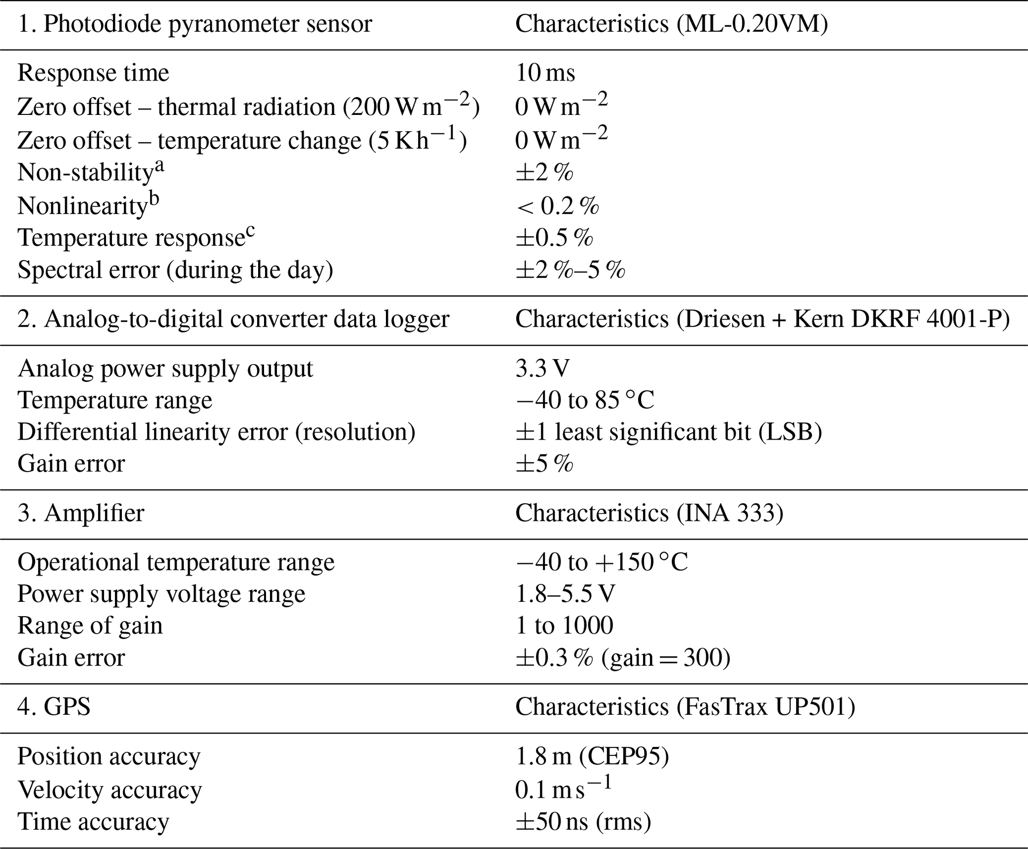
^a Percent change in responsivity per year.
^b Percent deviation from responsivity at 1000 W m⁻² due to change in irradiance %.
^c Percent deviation due to change in ambient temperature from −10 to 50 ^∘C.

It is worth mentioning that due to the large number of stations, a low-cost pyranometer was used, with an expected accuracy of about 5 % (see Table 1), which is substantially larger than measurement uncertainty achieved by state-of-the art secondary standard thermopile pyranometers. While ventilation and heating can additionally help improve data quality, in particular regarding dew, rain, and frost on the pyranometers, the power requirements for such measures made them unfeasible. It therefore needs to be stressed that the dataset is best suited for the investigation of spatial and temporal variability. Additionally, the data logger contained a Global Positioning System (GPS) antenna module (model: Fastrax UP501) for reliable time and position information.

The accuracy of the T_a measurements are ±1.5 ^∘C at −40 ^∘C, increase linearly to ±0.5 ^∘C at 0 ^∘C, and remain stable up to 40 ^∘C. Relative humidity observations were flawed due to sublimation occurring on the probe of the sensor. Therefore, the values of this parameter are not considered in this study and are not recommended for use. Finally, power for the system was supplied by a 6 V/19 Ah Zinc carbon VARTA 4R25-2 battery, allowing the system to work continuously for about 7 d.

2.1.1 Update of pyranometer calibration

In 2013, the pyranometers were calibrated with a standard spectrum solar simulator by EKO Instruments after their production (Madhavan et al., 2016). The stability of these factors is specified to be better than 2 % per year. Additional uncertainties are introduced in the measurement system by the data logger and the gain of the instrument amplifier (Madhavan et al., 2016). In order to update the calibration of the sensors and account for the spectral difference between a broadband pyranometer and the pyranometer network, intercomparison measurements were conducted in May 2018. The stations were set up in close vicinity to each other for 20 d on the roof of the main building at TROPOS in Leipzig, Germany. Out of this period, 2 h of observations were chosen on a clear-sky day (10:30–12:30 Z). These observations were compared to a recently calibrated secondary standard broadband thermopile pyranometer with a spectral range from 0.3 to 2.8 µm (model: Kipp & Zonen CMP21). After the comparison, the calibration coefficients were determined to minimize the difference between the network stations and the Kipp & Zonen pyranometer. The mean of the original calibration coefficients was 7.38 µV W⁻¹ m², while the updated calibration coefficients had a mean value of 7.19 µV W⁻¹ m². This suggests that, on average, the sensitivity of the instruments decreased slightly by 2.5 % over time. By updating the calibration, the root-mean-square error (RMSE) between the pyranometer stations and the reference pyranometer was reduced from 15.3 to 4.5 W m⁻², thus showing a significant improvement.

2.1.2 Quality assurance

The cleanliness of the sensor's glass dome and the horizontal alignment of the sensor leveling plate are important factors to guarantee the accuracy of the global horizontal irradiance (GHI) observations. In order to assure the quality of the dataset, the stations were checked daily, recording the status of the leveling and cleanliness. Each station contained a leveling spirit ring to indicate the alignment. The leveling criteria are based on the bubble position of the spirit level of the pyranometer. When the bubble was located inside the inner ring, the instrument was considered as well leveled, in between the two rings as partially leveled, and outside the ring as unleveled. Complete misalignment was found to occur when the base of rod was no longer properly supported by the snow due to melting, leading to a tilt of the sensor and systematic errors in particular for direct sunlight. Icing of the radiation sensor dome occurred when moist air masses with supercooled water droplets were present, which froze upon impact with the dome (Van den Broeke et al., 2004). This condition will generally lead to an underestimation of GHI.

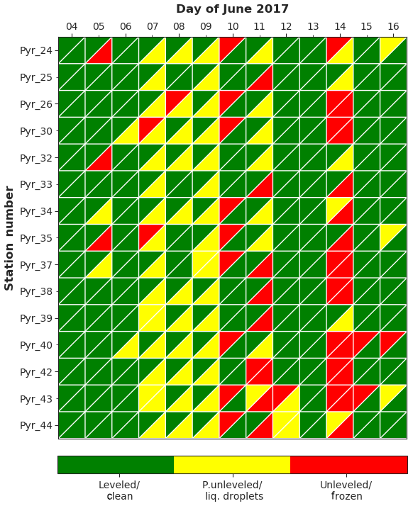
Figure 2 Quality flags for the pyranometer sensors: the pyranometer station number is shown on the y axis, and date is shown on the x axis. Each square is divided into two triangles: the upper shows the leveling flag and the lower the cleanliness status. Green is used for well-leveled and clean stations, yellow denotes partially unleveled stations or the presence of liquid droplets on the domes, and red is used for unleveled stations or iced domes.

Figure 2 shows the general status of the stations. Every station is shown on the y axis, while the date is given on the x axis. Each square is divided into two triangles, the upper one representing the leveling status of the station, and the lower one the cleanliness status. The green color shows a well-leveled and clean station, yellow is used for a partially leveled station or a dome with liquid droplets, and red is used for completely unleveled stations and an iced dome. Our following results do not make use of observations with iced domes or completely unleveled stations (red flags). The presence of liquid droplets is considered in the study due to their likely short residence time around the dome, and the fact that we have found observations to still be useful for our analysis. Furthermore, it is worth mentioning that during this likely short period, the presence of droplets is expected to cause a moderate underestimation of irradiance and more noisy observations.

It is nevertheless possible that the domes were contaminated by droplets or ice before or after the daily quality assurance checks. However, when significant fluctuations of atmospheric global transmittance (ATg) occurred, these were verified with observation by the all-sky camera operated on Polarstern. Such moments are discussed in the following sections.

2.1.3 Data processing

The raw data were stored by the stations in ASCII files in counts of 10 bits on an SD card. The records were subsequently converted to GHI (W m⁻²), air temperature (T_a in K) and relative humidity (RH in %) using the equations given in Madhavan et al. (2016). The values of GHI, T_a and RH were averaged to 1Hz sampling frequency according to the GPS time reference. The dataset was processed into NetCDF files following the latest 1.7 version of the Climate and Forecast Conventions (Unidata, 2012). Daily files containing all 15 pyranometer stations including GHI, T_a, RH, latitude (in degrees), longitude (in degrees), leveling and cleanliness flags, station number, and corrected calibration coefficient were prepared. Earth–Sun distance (in AU), solar constant, and solar zenith (θ in degrees) and azimuth angles (α in degrees) were added to the dataset based on the algorithms given in the World Meteorological Organization (WMO) Guide to Meteorological Instruments and Methods of Observations for practical application (WMO, 2008).

For our analyses, ATg was calculated from the GHI measurements following Eq. (1), where ϵ is the actual Earth–Sun distance (in AU), F_o is the solar constant, with a value of 1360.8 W m⁻² (Kopp and Lean, 2011), and μ_o is the cosine of the solar zenith angle (θ in degrees). ATg is hence defined as the fraction of radiation that is transmitted through the atmosphere (e.g., Liou, 2002).

$$\begin{array}{}\text{(1)}& \text{ATg}=\left[{\displaystyle \frac{F}{{\mathit{ϵ}}^{\mathrm{2}}\cdot F_{\mathrm{o}}\cdot {\mathit{\mu }}_{\mathrm{o}}}}\right]\end{array}$$

At the top of the atmosphere (TOA) ATg is 1, whereas at the bottom of the atmosphere (BOA) the value is reduced due to absorption and scattering within the atmosphere. At the BOA the highest values are generally observed for cloudless conditions, while clouds generally cause a reduction of ATg. Under certain situations, however, the presence of broken clouds can amplify ATg to reach values larger than 1 due to horizontal photon transport and 3D radiative effects. Such enhancements can exceed 400 W m⁻² and persist up to 20 s (Schade et al., 2007).

2.1.4 Sky classification

To analyze the effect of clouds on the ATg, a general overview of cloud conditions was first obtained. An overview of the cloud conditions present during PASCAL was already given by Wendisch et al. (2019). Whereas their classification was based on time–height cross sections of clouds classified from vertical-stare active and passive remote sensing observations, the classification used here is based on the visual inspection of all-sky camera observations recorded aboard Polarstern. These images provide a more complete impression of the horizontal variability of clouds, which is important for the characterization of inhomogeneities of the atmospheric transmittance. Initially, a separation of overcast, cloudless and broken cloud conditions was made from the all-sky camera observations on Polarstern. Due to the availability of observations with a cloud radar of type Mira-35, and multiwavelength polarization Raman lidar Polly-XT (Engelmann et al., 2016) during PASCAL (Wendisch et al., 2019; Macke and Flores, 2018), these were used in addition to identify the presence of multilayer clouds, a separation which has not been considered in previous studies (Madhavan et al., 2016, 2017; Lohmann et al., 2016; Lohmann and Monahan, 2018). Cirrus clouds and low, geometrically thin stratus clouds were also observed and have been considered together as thin clouds due to their low occurrence frequency to study their effects on ATg.

The final classification was made considering the daily quicklooks of the range-corrected signal at 532 and 1064 nm wavelength from the lidar, daily plots of the radar reflectivity, and images from the all-sky camera. Whenever the lidar signal was attenuated, the information of the cloud radar was used to identify the presence of single or multiple layers of clouds. For apparently clear-sky moments, as identified by the lidar and radar quicklooks, images from the sky camera were used to confirm the absence of clouds, or to identify thin cloud layers or broken cloud situations. In this study, conditions were only considered to be cloudless when the images from the all-sky camera did not show any clouds within its fish-eye field-of-view. The transition from one type of sky condition to another was only recorded when this class lasted for longer than 15 min. Cases when the change was observed for less than 15 min were assumed to belong to the previous sky condition. Thin clouds were defined as clouds with a height difference between the cloud base and cloud top of below 450 m. The result of this classification is shown by the color coding in Fig. 4, and examples for each condition are shown by all-sky camera images for each case study.

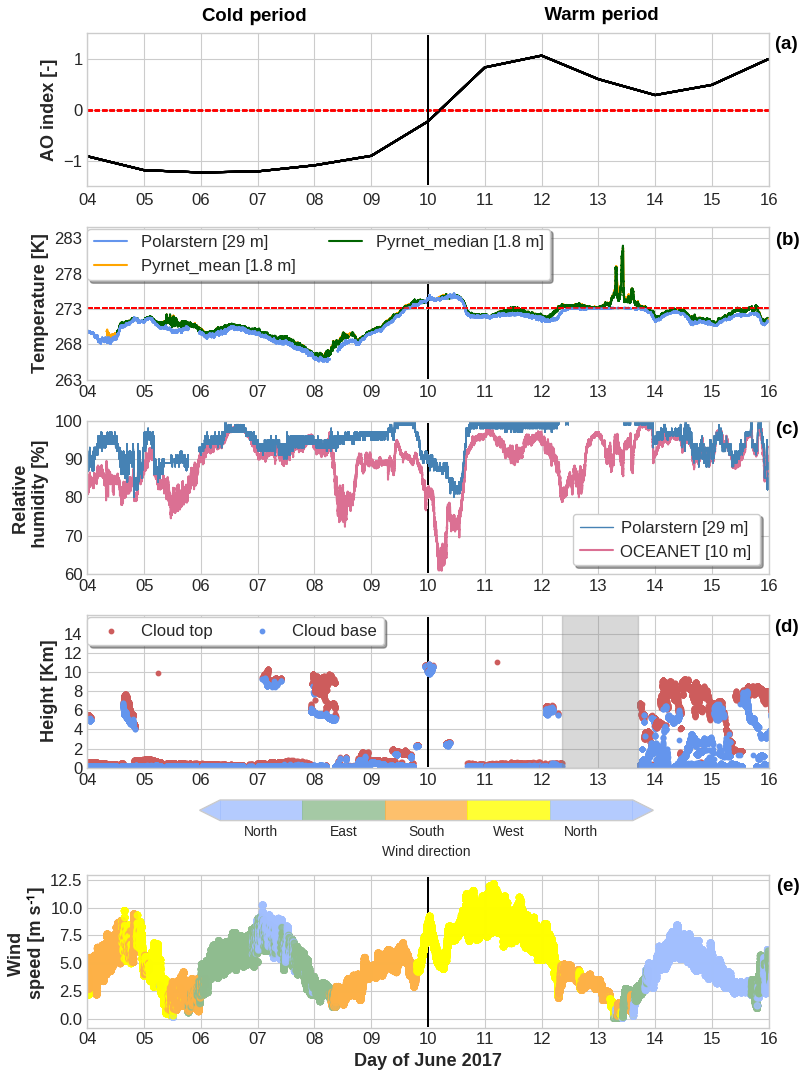
Figure 3 (a) AO index reported by the National Oceanic and Atmospheric Administration (NOAA). (b) Surface temperature from Polarstern meteorological instruments (blue), together with the mean (orange) and median (green) values from the pyranometer network. (c) Relative humidity (RH) from Polarstern (blue) and from the OCEANET container (pink). (d) Cloud base and cloud top height based on cloud radar and lidar. The gray background marks moments with no observations. (e) Wind speed (m s⁻¹) and direction obtained from Polarstern observations.

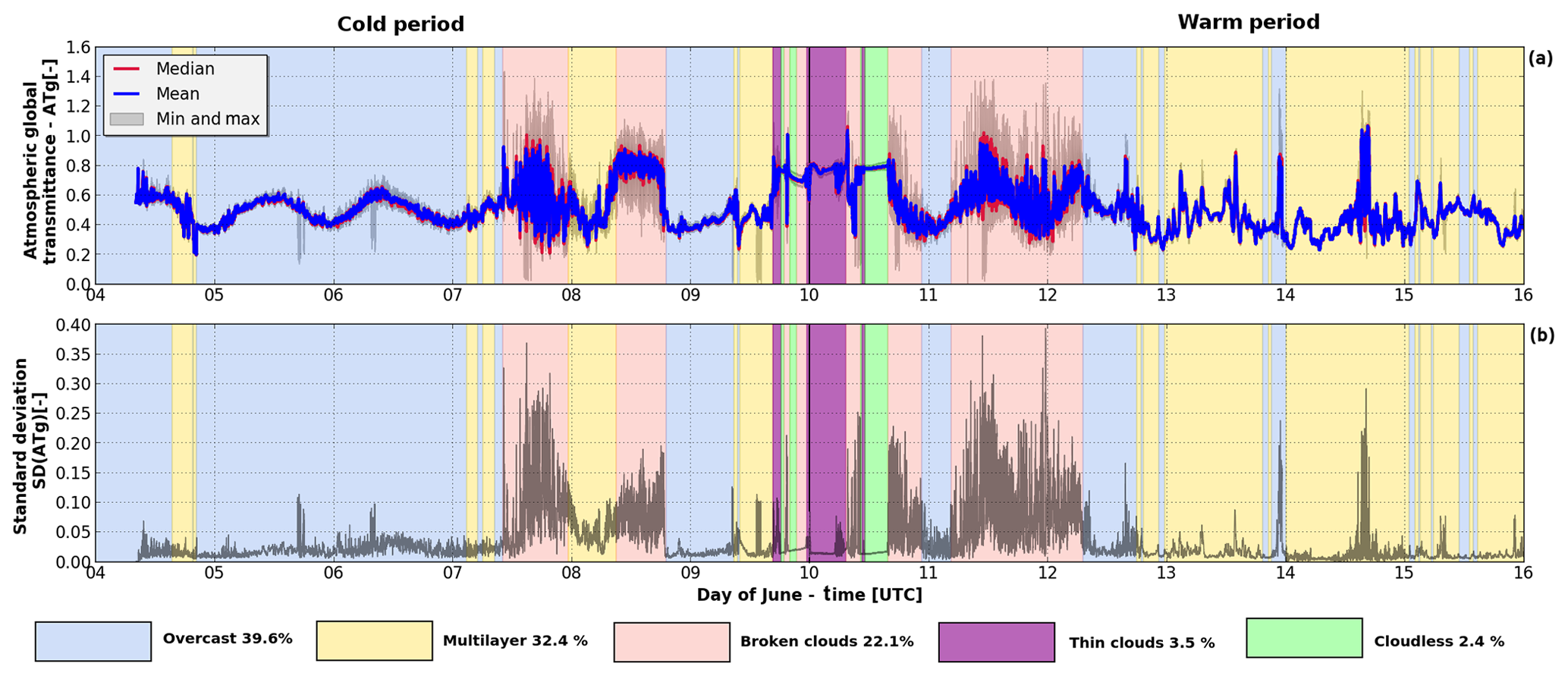
Figure 4 (a) Time series of atmospheric global transmittance (ATg) derived from the pyranometer network. (b) Time series of the inter-station standard deviation of ATg.

3 Results

In this section, results obtained from an analysis of the pyranometer network observations are presented. First, the synoptic conditions during the ice floe camp are described, and related to the observations of atmospheric transmittance under specific sky conditions. Case studies pertaining to each of the used sky conditions are presented next. Finally, the difference in power spectra for these sky conditions obtained from a wavelet-based multi-resolution analysis of atmospheric transmittance are discussed.

3.1 Near-surface temperature classification during PASCAL: ice floe camp and synoptic implications

A detailed synoptic-scale description for PASCAL is provided in Knudsen et al. (2018), where a longer period covering the airborne activities of the ACLOUD campaign is analyzed. Based on near-surface and upper-air meteorological observations and operational satellite and model data, three periods were characterized (warm, cold, and normal periods). The PASCAL observations at the ice floe camp took place mainly in the warm period, 30 May to 12 June, when warm and moist maritime air intruding from the south and east dominated the synoptic conditions. However, the classification by Knudsen et al. (2018) considers a larger spatial scale that neglects sensitive local episodes at the ice floe camp which need to be considered when analyzing the near-surface temperature changes at the ice floe camp. Therefore, the classification has been sharpened for the limited period of the ice floe camp considering the near-surface temperature (Fig. 3b).

With the aim of considering the influence of the large-scale Arctic circulation on the synoptic conditions during the ice floe camp, the Arctic oscillation index (AO) is used in our analysis here. It refers to an opposing pattern of pressure difference between the Arctic and the northern midlatitudes.

The AO is a climate index which characterizes the atmospheric circulation of the Arctic region by considering geopotential height anomalies of the 1000 mb isobar between 20 and 90^∘ N. It is defined as the loading of the dominating mode obtained from an Empirical Orthogonal Function (EOF) analysis of the monthly mean anomaly fields. Here, daily values of the AO index as reported by the Climate Data Center of the National Oceanic and Atmospheric Administration are used (source: ftp://ftp.cpc.ncep.noaa.gov/cwlinks/, last access: 20 March 2020). To determine the loadings, the current height anomaly from the monthly average field is projected onto the pattern of the leading EOF mode, which has been determined from monthly averages obtained from the NCEP and NCAR reanalysis for the period 1970–2000.

A positive AO index generally corresponds to strong westerly winds in the upper atmosphere, lower than usual atmospheric pressures and temperatures in the Arctic, and an opposite effect on pressure and temperature midlatitudes. On the other hand, a negative AO index leads to weaker upper-level winds, higher atmospheric pressure and warmer temperatures in the Arctic, and contrary effects and an increase in storms in the midlatitudes (Thompson and Wallace, 1998).

A classification is presented considering the near-surface air temperature (Fig. 3a) and contrasting it to the AO index (Fig. 3b). One can distinguish two main periods. First, from 4 to 9 June 2017, a cold period was observed with relatively low near-surface air temperatures (mean: 269.7 K). The negative AO index suggests a reduction in the difference of surface pressure between the Arctic and northern middle latitudes, resulting in a larger polar low-pressure system and warmer-than-usual temperatures (Talley et al., 2011). From 10 to 16 June 2017, a warm period can be identified due to an increase in temperature (mean: 272.32 K). The temperature reaches two maxima on 10 and 13 June. A positive AO index is generally associated with colder-than-usual temperatures, stronger westerly winds in the upper atmosphere, and a more cyclonic circulation that can influence sea ice motion (Rigor et al., 2002). The classification made is solely based on the near-surface air temperature and the AO index reveals the synoptic patterns considering the interannual variability.

Figure 3c shows that humid conditions prevailed during most of the ice floe camp, with a notable drop in relative humidity during the transition between the cold and the warm period. Two relative humidity (RH) sensors were operated at different heights on Polarstern. One sensor was mounted on top of the OCEANET facility OCEANET at about 10 m above sea level, while the second one was installed on the crow nest of Polarstern at a height of 29 m. The discrepancies in the observations of both sensors are mainly due to the different heights and locations of the sensor. The Polarstern sensor, a Vaisala sensor of type HMP155 (accuracy: $<\pm \mathrm{5.0}$ % RH), was exposed to more open conditions, whereas the OCEANET sensor of type EE33 (accuracy: ±1.3 % RH) was relatively protected (explanation from Henry Kleta of the Deutscher Wetterdienst, DWD). Considering the RH values obtained by the Polarstern sensor, the mean RH during the first period was 94 %, and 95.7 % for the second. On 10 June 2017, the longest cloudless period occurred, and the RH observed by the Polarstern sensor dropped to 80 %. After this event, a moist air intrusion was observed already in the evening of 10 June (Knudsen et al., 2018).

About 97.2 % of the time, cloudy skies were observed during the ice floe camp. Low-level clouds with cloud tops no higher than 2.6 km and a mean cloud base of 220 m above the surface were observed. During the cold period, mostly overcast conditions with single-layer clouds were present, whereas multilayer and broken clouds dominated the second period (Fig. 4).

During the first and the second period, mean wind speeds of 4.77 and 5.32 m s⁻¹, respectively, were observed (Fig. 3e). Four maxima in wind speed were observed during the ice floe camp, on 4 June with southerly winds, on 7 June with northerly and easterly winds, on 11 June with southerly winds, and on 14 June with northerly winds (Fig. 3d and e).

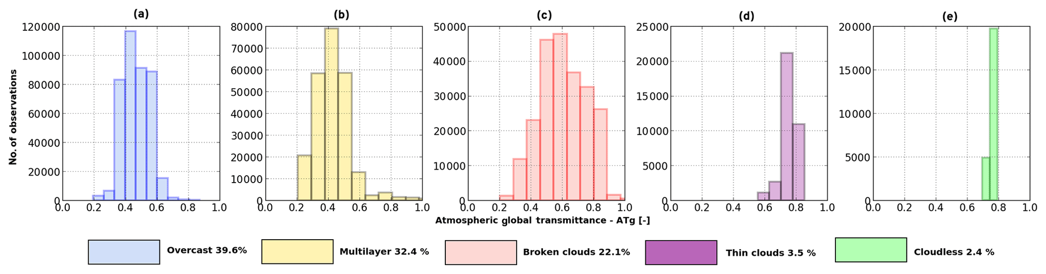
Figure 5 Histograms of atmospheric global transmittance (ATg) for (a) overcast, (b) multilayer, (c) broken cloud, (d) thin cloud, and (e) cloudless sky conditions.

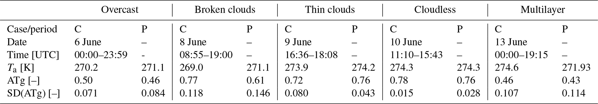
Table 2 Mean values of ambient temperature T_a [K] and atmospheric global transmittance ATg [–] for case studies (C) and all periods (P). All results are based on the pyranometer network.

3.2 Meteorological classification of global transmittance

Using the methodology introduced in Sect. 2.1.4, Fig. 4a shows the time series of the ATg for the whole period of the ice floe, and considering all operational pyranometers. Figure 4b shows the time series of the inter-station standard deviation (SD), and Fig. 5 presents the histograms for each of the sky conditions.

As can be seen in Fig. 4, about 40 % of the time overcast conditions dominated the ice floe camp, occurring mainly during the cold period. This sky condition resulted in ATg values generally lower than 0.7, with a mean value of 0.46 (Fig. 5 and Table 2). The monomodal distribution of ATg was mainly characterized by stratus clouds; however, during 9 and 11 June, the presence of stratus nebulosus clouds was observed due to the formation of rain or drizzle as visible from the all-sky camera.

Multilayer clouds, mainly consisting of double layers (Figs. 3d, 4a), occurred about 30 % of the time. They again caused a monomodal distribution of ATg, with a mean value of 0.43 (Fig. 5 and Table 2). This sky condition was more frequently observed during the warm period. The time–height cross section of the radar reflectivity revealed complex structures of three layers of clouds on 13 and 14 June and two layers reaching up to 9 km height observed on 15 June. On 9 June from 09:50 to 12:00 Z and from 12 June at 19:20 Z to 13 June at 09:15 Z, precipitation was observed by the all-sky camera. During this episode, it is possible that the domes of the pyranometer were covered with small droplets which might not have been present at the moment of daily quality control.

The third most frequent sky condition corresponded to broken clouds (22.1 %). This sky condition was present during both the cold and the warm period, and it showed subtle differences that complicated its classification. The data taken on 7 June had less frequent cloud gaps than other days. The sky was covered by stratus fractus clouds as seen in Fig. 13a at 12:06 Z. The data taken on 8 June showed a combination of cumulus fractus (Fig. 13b at 10:14 Z) and stratus fractus clouds. At the end of 10 June, broken cloud conditions were observed, corresponding also mainly to stratus fractus clouds. On 11 and 12 June, sky conditions were similar to 7 June, with slight precipitation from 11 June at 21:15 Z to 12 June at 01:10 Z. The ATg observed for broken clouds had a monomodal distribution and a relatively high mean ATg of 0.61, with a SD of 0.146 (Figs. 4, 5, and Table 2).

The selection of thin cloud conditions was rather complex, due to their similarities with broken clouds and because they frequently occurred outside the field of view of the lidar. For these cases, the classification was based entirely on the all-sky camera. On 9 June, a fairly uniform stratus cloud was observed from 16:35 to 18:08 Z and from 23:24 Z to 10 June at 07:18 Z, when cirrus fibratus clouds at 10 km height occurred. Thin cloud conditions appeared only during the transition period, with a frequency of only 3.5 % (Fig. 3) and a mean ATg of 0.76 (SD 0.043). Finally, the least frequently occurring condition with only 2.4 % of occurrence frequency was cloudless sky, with a monomodal distribution and a mean ATg of 0.76 (SD of 0.028). This sky condition only occurred at the end of 9 June, and on 10 June from 11:10 to 15:43 Z.

The following subsections analyze particular case studies for the different sky conditions discussed. The analysis takes into account the temporal standard deviation of ATg of the stations with reliable observations, the histogram of the distribution of global transmittance, a map for comparing the spatial patterns of the standard deviation, a wind rose to indicate the wind speed and direction, and a photograph of the all-sky camera to visualize the corresponding cloud structure.

3.3 Cloudless case – 10 June 2017

The day with the longest cloudless period was 10 June 2017 (11:10–15:43 Z). This episode also coincides with the beginning of the warm period (Sect. 2.1), with a mean ambient temperature of 274 K. This day was also characterized by the warmest air in the upper atmospheric layers during the ice floe period, and a relatively low boundary layer of about 200 m height (Knudsen et al., 2018).

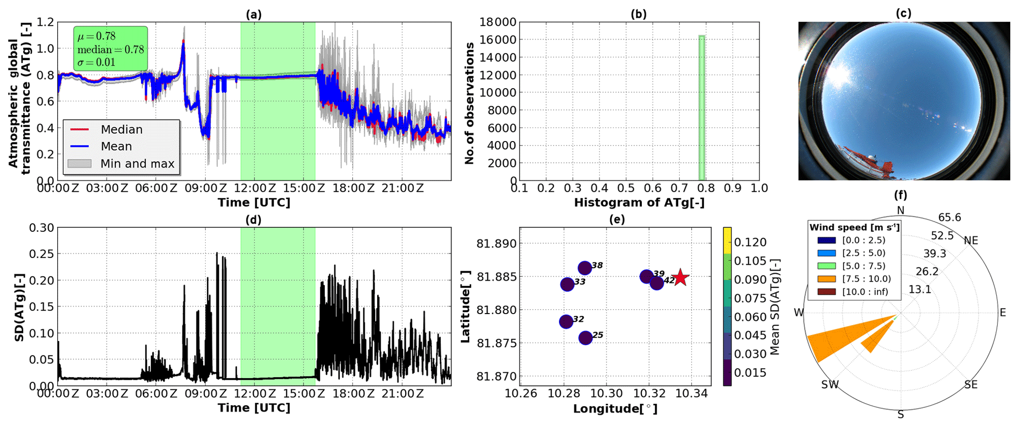
Figure 6 Overview of the cloudless case: panel (a) shows the time series of atmospheric global transmittance (ATg), and the green-shaded background marks the cloudless period (10 June 2017, 11:10–15:43 Z). (b) Histogram of global transmittance for cloudless conditions. (c) Photograph from the all-sky camera at 13:51:44 Z. (d) Time series of the inter-station standard deviation (SD) of ATg based on all functional stations. (e) Map of the stations showing the temporal SD for individual stations, while the red star marks the position of Polarstern. (f) Wind rose for the selected period.

The positive AO index (Fig. 3a) suggests dry conditions (Fig. 3c) associated with an anticyclonic circulation (Knudsen et al., 2018), leading to reduced cloudiness and enhanced downward solar radiation (Kay et al., 2008). Figure 6a shows the time series of the global transmittance, and the green background highlights the cloudless period. In Fig. 6b, the narrow distribution of ATg is shown, with values just below 0.8. The comparatively small reduction of transmittance is mainly due to scattering and absorption by atmospheric gases, and, to a lesser degree, due to aerosols. In early spring or autumn, lower values of ATg are expected due to the lower sun and the resulting longer optical path through the atmosphere (Zhao and Garrett, 2015). The temporal standard deviation of the operational pyranometers is shown in Fig. 6d, having a mean value of 0.014 for the period of interest. Figure 6d shows the standard deviation of the measurements for each pyranometer during the selected period. Variability in the observed global transmittance is mainly noticed for stations 39 and 42, with a standard deviation of 0.0090 and 0.0092, respectively. It is likely that this variability can be attributed to undetected deficiencies such as an unleveled instrument due to melting.

3.4 Overcast case – 6 June 2017

The overcast case selected occurred on 6 June between 00:00 and 23:59 Z. During this day, the boundary layer increased in height from 300 m to about 430 m. This day was characterized by a mean cloud base and cloud top of about 100 and 490 m, respectively (Wendisch et al., 2019). The wind speed measured on board Polarstern increased from 2.5 m s⁻¹ to almost 10 m s⁻¹ in the evening with easterly origin (see Figs. 3e and 7f). The mean surface temperature recorded by the pyranometer network during this period was 270.1 K, with an inter-station SD of 0.38 K.

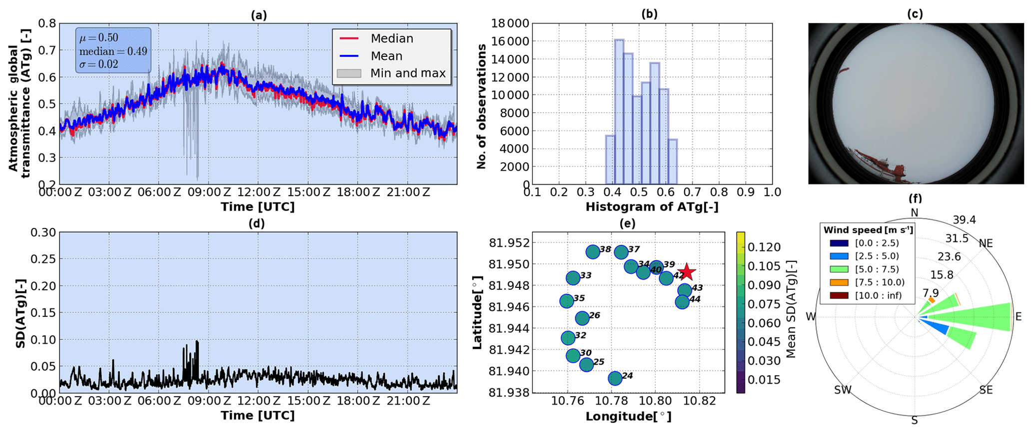
Figure 7 Overview of overcast case: the same as Fig. 6 but for 6 June 2017, 00:00–23:59 Z. All-sky camera photograph taken at 13:41:54 Z.

The ATg during this period showed a monomodal distribution (Fig. 7b), with a mean value of 0.50. The time series of the standard deviation presented values lower than 0.1 (mean SD=0.023), as well as high values from 07:29 to 08:27 Z, when the dome of the instruments might have experienced momentary icing (Fig. 7d). The stations showing this behavior were 26, 30, 34, 35, 38, 40 and 43. The spatial distribution of the SD shows slightly higher values in the southwest of the ice floe region (Fig. 7e). This small variance is most likely attributed to a more snowy surrounded area, whereas pyranometers 37, 34, 40, 39, 42, 43 and 44 were closer to the ice edge (Fig. 1b). Snow-covered surfaces reflect more solar radiation to the atmosphere than darker surfaces such as the open ocean. Once this reflected energy reaches a cloud, a part of it is reflected back to the surface, increasing the total amount of downward solar radiation. Thus, for homogeneous single-layer clouds, the stations closer to the ice edge show lower variation because more energy is absorbed by the darker surface.

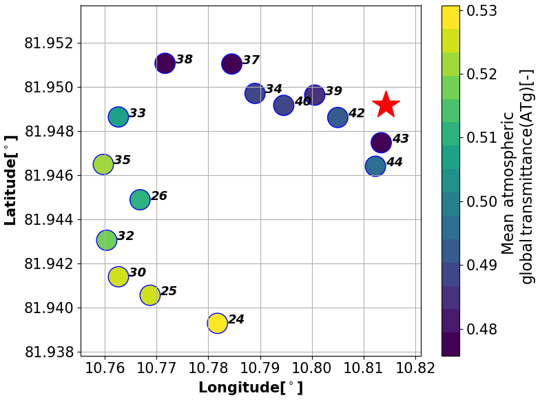
Figure 8 Station map showing the average atmospheric global transmittance for the overcast case (6 June 2017, 00:00–23:59 Z). The red star marks the position of Polarstern.

In addition, Fig. 8 shows the spatial distribution of the mean ATg. It clearly shows how stations near Polarstern (red star) and the edge of the ice floe observe lower values of transmittance than the stations farther away from the ice edge, with absolute differences ranging up to 0.06. A likely explanation is the low surface albedo of the open water, which leads to a reduction in multiple reflections between the ground and cloud base compared to those stations fully surrounded by snow-covered ground. A similar plot was made for 5 June, where the sky conditions were also overcast. A similar but less pronounced pattern was observed (not shown) with a smaller difference of up to 0.03.

3.5 Thin clouds case – 9 June 2017

Thin clouds were not frequent during the ice floe camp period. The only cases occurred on 9 and 10 June (Wendisch et al., 2019). The thin cloud case selected for the case study was observed between 16:36 and 18:08 Z on 9 June. The overall cloud conditions during this period were complex because the clouds varied in both height and depth (see Fig. 3). From 16:30 to 17:00 Z, a single cloud layer with a base height of 1.1 km and top height of 1.5 km was observed. During this period, drizzle was observed at the cloud base. Following this period, a very shallow cloud was observed with a cloud top of about 0.45 km from 17:00 to 18:05 Z.

Figure 9 Overview of thin cloud case: the same as Fig. 6 but for 9 June 2017, 16:36–18:08 Z. All-sky camera photograph taken at 17:29:28 Z.

The mean ambient temperature during this period was 273.9 K with a SD of 0.35 K. During this condition the cloud base height was at 450 m and the temperature increased steadily from 273.15 to 274.11 K. The winds came mainly from the south, following an anticyclonic circulation with mean wind speeds of 5.2 m s⁻¹ (Knudsen et al., 2018, Figs. 3e, 9f). The variance of height and composition had an impact on the ATg and temperature measured by the pyranometer network, as can be seen in the shaded purple background in Fig. 9a. The highest values of inter-station SD occurred at the moment when the optical thickness of the cloud decreased at 17:30 Z. The mean ATg during this period was 0.72, with a left-skewed distribution (see Fig. 9b). The spatial distribution of the SD shows a similar trend as in the overcast case. This suggests that during these conditions, the highest variability occurred in the region away from the ice floe edge and melt pond (Fig. 1b). The spatial distribution of mean transmittance shows a less evident pattern, suggesting that part of this variability is caused by variable cloud structures more than due to the particular location of the stations. The highest difference of the mean transmittance between all operational stations is 0.08.

3.6 Multilayer case – 13 June 2017

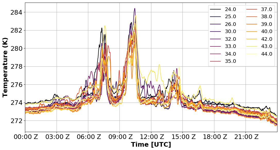
The multilayer case selected was 13 June 2017, from 00:00 to 19:15 Z. This day had a positive AO index, implying that the episode was dominated by an anticyclonic circulation, when air was advected over the open ocean, favoring high temperature and humidity (Knudsen et al., 2018, Fig. 3a). Wind speeds were below 5 m s⁻¹ coming from the southwest and northeast (see Figs. 3e and 10f). The RH was rather unstable, varying from 85 % to 96 % at 10 m height and close to 100 % at 29 m height (Fig. 3c).

The warmest day of the ice floe camp was 13 June. At around 07:30 and 10:15 Z, the highest temperatures of 279.03 and 281.1 K were recorded (see Fig. 11). This increase in temperature was not recorded by the Polarstern temperature sensor (see Fig. 3b). The observed fluctuations suggest that the near-surface air temperature over the ice floe experienced significant variability, likely due to turbulent mixing with warmer, elevated air masses. A spatial comparison among the sensors of SD and mean near-surface temperature did not indicate a particular pattern but showed relatively high differences of mean temperature of up to 1.4 K.

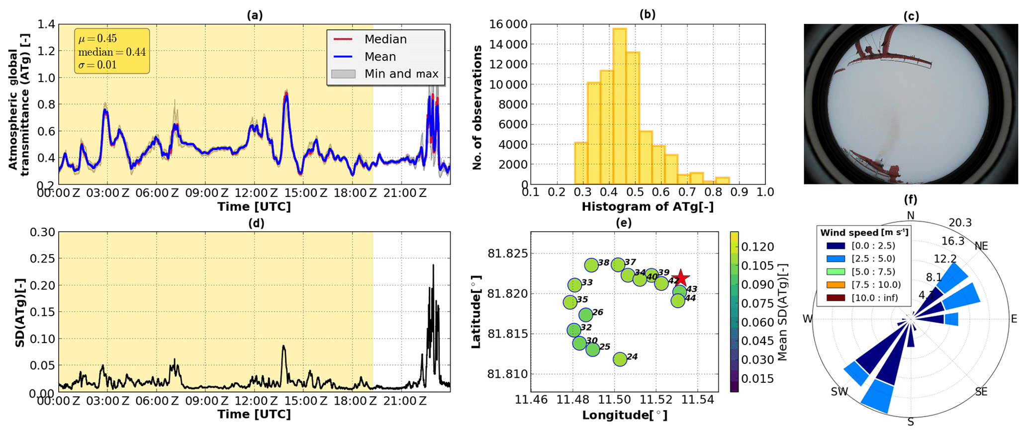
Figure 10 Overview of multilayer case: the same as Fig. 6 but for 13 June 2017, 00:00–19:15 Z. All-sky camera photograph taken at 10:09:35 Z.

Figure 11 Time series of 1 min averaged temperature for all stations on 13 June 2017.

From 00:00 to 02:24 Z, three layers of clouds were identified with tops at 0.9, 4.8 and 7.8 km. The remaining time of the period was characterized mainly by complex structures, and two cloud layers showed low values and a right-skewed distribution, having a mean of 0.45 (SD 0.0165). The variation observed is mainly attributed to the different vertical structure of the multiple cloud layers (see Fig. 10b, Table 2). The time series of ATg and inter-station SD indicated no significant variation among the stations (Fig. 10a and d). Furthermore, the values of temporal SD found for the individual stations do not show a prominent spatial variation as, for example, observed for the overcast and thin cloud cases (Fig. 10e). Considering that the difference between the lowest and the highest value of SD is low (0.007), the variation in the GHI for this case is negligible.

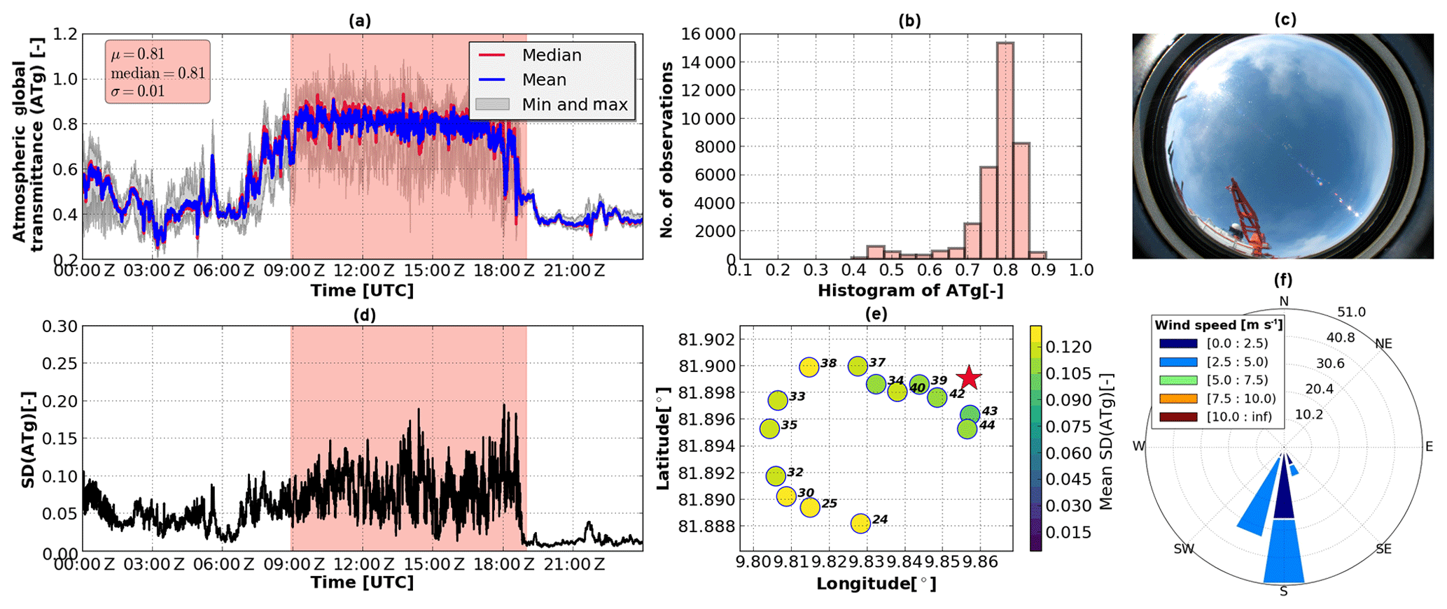
Figure 12 Overview of broken cloud case: the same as Fig. 6 but for 8 June 2017, 08:55–19:00 Z. All-sky camera photograph taken at 12:41:14 Z.

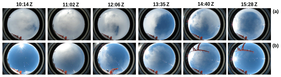
Figure 13 All-sky camera photographs for (a) 7 June and (b) 8 June, taken at different times throughout the day.

3.7 Broken clouds case – 8 June 2017

The period from 08:30 to 18:59 Z of 8 June 2017 was characterized by fluctuating occurrences of stratus fractus (Fig. 13b at 11:02 Z) and cumulus fractus (Fig. 12c). During this case, southeasterly winds with a mean speed of 2.6 m s⁻¹ prevailed (Figs. 3c and 12f). A remarkable drop of relative humidity was observed by the OCEANET sensor at 10 m height at around 12:00 Z, whereas the values at 29 m height remained stable (Fig. 3c). Near-surface air temperatures observed with the pyranometer network increased by 2 K from 267 to 269 K. This behavior was also recorded by the Polarstern sensor (Fig. 3b). Before the broken cloud conditions began, the temperatures recorded were the lowest registered during the entire campaign.

The pink-shaded background in Fig. 12a and c highlights the broken cloud period. The mean and median ATg is represented in Fig. 12a in blue and red, respectively. The gray spikes represent the minimum and maximum values recorded for each time, indicating that, for instance, the transmittance varied from 0.4 to 1 (and above) for a few stations. The increase in diffuse solar radiation is attributed not only to the broken cloud conditions but also to the multiple reflection between surface and heterogeneous cloud fields. Under these conditions, the plane-parallel cloud approximation cannot satisfactorily describe radiative transfer (Wendler et al., 2004; Schade et al., 2007). In particular, it is well known that horizontal photon transport can lead to periods with enhanced solar radiation, where values of the global transmittance can exceed the clear-sky values or even unity for some moments (Schade et al., 2007). In addition, Byrne et al. (1996) demonstrated that in broken cloud fields, the average photon path length is greater than that predicted by homogeneous radiative transfer calculations, also leading to an enhanced absorption.

Based on the mean values of ATg for this period, the histogram in Fig. 12b shows a left-skewed distribution and a mean value of 0.81, with a mean standard deviation of 0.01. Fluctuations of the standard deviation can be easily recognized in Fig. 12d, with more noticeable spikes before and after the selected period. The spatial variability, shown in Fig. 12e, indicates higher values of temporal standard deviation for the stations further away from the ice floe edge; however, the mean ATg does not show the same pattern as in Fig. 8. The latter may indicates that the variability observed is dominated by the cloud organization and not by the contrast between the open ocean and highly reflective surfaces.

3.8 Wavelet-based multi-resolution analysis

To investigate the timescale dependence of variability in global irradiance, the time series of ATg obtained from the pyranometer network have been subjected to a wavelet-based multi-resolution analysis using the Haar wavelet, following the methodology introduced in Deneke et al. (2009) and Madhavan et al. (2017). In summary, J=13 low-pass-filtered versions of the time series are calculated first, using a running mean of length L=2^J as a filter. In wavelet analysis, these running means are referred to as the wavelet smooths. The difference between two wavelet smooths of scale J and J+1 correspond to the result of a bandpass filter and are called wavelet details. The wavelet details are then used to obtain time-localized estimates of the timescale-dependent variance of the time series (Percival, 1995), which is denoted as the wavelet power spectral density (WSD).

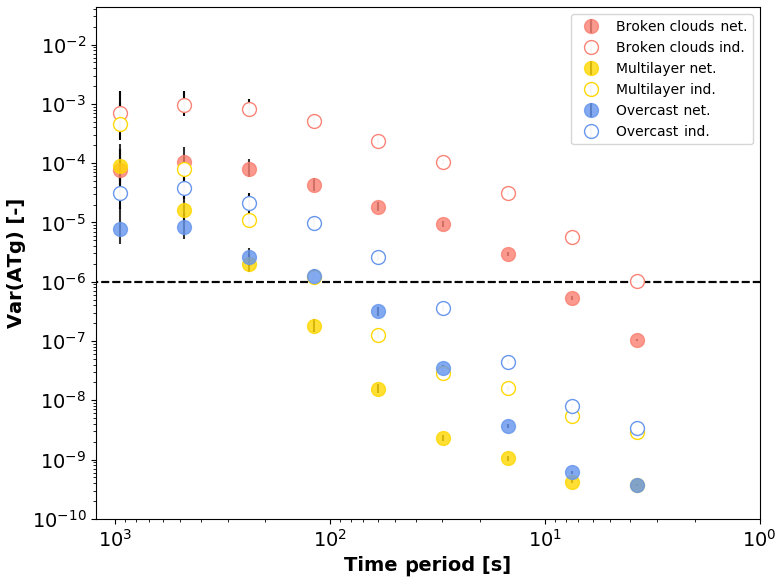
Figure 14 Wavelet-based power spectral density (WSD) of the station-averaged ATg (filled circles) and averaged WSD from the individual stations (empty circles) for 3 h periods (15:00–18:00 Z) with broken cloud (8 June 2017), multilayer (13 June 2017), and overcast (6 June 2017) conditions. The dashed horizontal line denotes the measurement uncertainty of the pyranometer.

Figure 14 shows the WSD obtained from the observations for a period of 3 h of broken cloud, multilayer cloud, and overcast conditions from 15:00 to 18:00 Z for the case days presented previously, in a double-logarithmic plot, and includes estimates of its uncertainty. Figure 14 compares the WSD calculated in two different ways. Filled circles correspond to the WSD, which has been calculated based on the average ATg of all functional stations, which approximates the WSD of ATg averaged across the spatial domain of the network, with a characteristic length scale of about 1 km. Empty circles correspond to the averaged WSD of individual stations and thus a point-like measurement. Due to the 3 h length of the time series, the WSD for periods at and above 1000 s cannot be reliably observed, as is evident from the increasing uncertainty.

A characteristic decrease in variance with increasing temporal frequency (or equivalently, a decreasing time period) is observed for the different sky conditions. In particular, strongly differing slopes of the WSD are observed for the different conditions and frequency ranges, which suggests that the WSD is sensitive to structural differences of the clouds. As noted already by Madhavan et al. (2017), variability is significantly reduced when considering the spatially averaged atmospheric transmittance, irrespective of the considered cloud type. Broken clouds exhibit the largest variability, while the multilayer cloud situations show the smallest variability across all timescales.

In Fig. 15, the WSD for two different periods classified as broken clouds are compared. As noted before, on 7 June, stratus fractus were observed, with stronger winds likely responsible for stronger fluctuations and longer periods of cloud-free sky, while the broken clouds observed on 8 June, corresponding to a mixture of cumulus fractus, stratus fractus and stratocumulus, introduced less fluctuations in ATg. The lower variability can already be seen in Fig. 4b. It is noteworthy that spatial averaging has a much stronger effect on the magnitude of variability for the 8 June case, which indicates that the relevant variations in cloud properties occurred on length scales smaller than the extent of the pyranometer network, while a much smaller reduction is observed for 7 June. This indicates that cloud scales larger than the extent of the pyranometer network dominated the variability in transmittance during this period.

As noted previously by Madhavan et al. (2017), a stronger scale dependency can be recognized in the WSD for the broken clouds observed on 8 June compared those of 7 June. Estimating the slope of the WSD from the four points above and below a period of 100 s, slopes of the WSD of 1.5 and 1.7 are obtained for 7 June, while much lower values of 0.9 and 1.0 are found for 8 June, for spatially averaged and point observations, respectively. Here, the values for 7 June are close to the theoretical exponent value of 5 / 3 expected from turbulence theory for the dissipation of energy expected from homogeneous isotropic turbulence, while the lower values are in better agreement with the values reported by Madhavan et al. (2017) for broken cloud observations.

Comparing Figs. 14 and 15, differences of the WSD for the average of all functional stations (filled circles) and considering the individual point-like measurements (empty circles) can be seen, indicating that the variability is reduced by about 0.1 as the spatial averaging cancels out part of the small-scale spatial variability. Hence, spatial averaging of stations allows us to better resolve temporal changes, while the magnitude of the difference provides information on the small-scale spatial structure of clouds. The results obtained here also suggest that future measurements of GHI in similar highly reflective surface conditions should be done with a temporal resolution of at least 10 s to fully capture the variability under broken cloud conditions. This conclusion corroborates the findings of Lohmann and Monahan (2018) that, based on HOPE-Jülich campaign, suggest increasing the current recording of solar irradiance from 1 min resolution, as recommended by the Baseline Surface Radiation Network (BSRN) (McArthur, 2005), to a much higher temporal resolution.

4 Discussion, conclusion and outlook

Over the past few years, the Arctic has been experiencing an unprecedented increase in surface temperature and an associated decrease in sea ice extent, by far exceeding model-based climate projections. Scientific efforts to identify and understand the mechanisms that contribute most to this Arctic warming are still ongoing (Serreze and Francis, 2006; Serreze and Barry, 2011; Vihma, 2014; Wendisch et al., 2017). After the two extreme events with very low sea ice in 2007 and 2012, the debate to explain these events was principally divided into two sides. Several studies suggest that meridional heat transport is a main contributor to the Arctic warming (Nussbaumer and Pinker, 2012; Graversen et al., 2011). On the other hand, several studies propose that anomalies in the solar radiation budget and clouds contribute to sea ice loss during summer (Kay et al., 2008; Pinker et al., 2014).

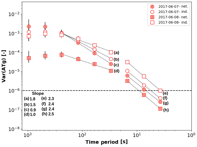
Figure 15 Wavelet-based power spectral density (WSD) of the station-averaged ATg (filled circles) and average WSD from the individual stations (empty circles) for 3 h periods (15:00–18:00 Z) of broken clouds on 7 June (circles) and 8 June (squares). Solid lines indicate the linear regression for the time period selected, and the dashed horizontal line correspond to the measurement uncertainty of the pyranometer.

As one specific aspect of the solar radiation budget, the present study focuses on the analysis of the spatiotemporal variability of the solar atmospheric transmissivity at the surface as it is introduced by clouds. Despite the fact the silicon photodiode pyranometers used in this study operate with a limited spectral range of 0.3–1.1 µm and thus do not cover the entire solar spectral range like a conventional broadband thermopile pyranometer, they do capture the main changes of the solar spectral transmission induced by clouds (Bartlett et al., 1998). Therefore, it is worth stressing that the analysis of the spatiotemporal variability induced by clouds in the shortwave infrared region (e.g., in the atmospheric windows at 1.6 or 2.2 µm commonly used for satellite remote sensing) is outside of the scope of this study, and might be a valuable investigation for future research.

To support our analysis, the characterization of synoptic conditions given by Knudsen et al. (2018) is used as a basis. Focusing on the near surface air temperature, we identified a cold period from 4 to 9 June 2017 and a warm period from 10 to 16 June 2017. Although the classification labels the first period as cold, the AO index indicates that atmospheric conditions were warmer than average. In contrast, atmospheric circulation over the Arctic for the warm period featured stronger westerlies at subpolar latitudes and lower sea level pressure over the Arctic (Thompson and Wallace, 1998; Rigor et al., 2002).

During the cold period, overcast conditions with single-layer clouds prevailed, with air masses coming mainly from the east and south. The mean ATg during overcast conditions was relatively low (0.48). The warm period was mainly dominated by multilayer clouds, with a mean ATg of 0.41, and with winds mainly coming from the west and north. The distribution and temporal variability of ATg for overcast and multilayer clouds were found to be similar. However, the distinction is important since overcast conditions represent more clearly the diurnal cycle and the spatial distribution of the stations showing a specific pattern. Broken clouds were observed during both periods and for wind speeds higher than 4 m s⁻¹ and air masses coming from the north and east for the cold period and from the west during the warm period. The mean observed ATg for broken clouds was 0.61, and showed the highest temporal variability.

Wavelet-based power spectra showed pronounced differences for different sky conditions, with highest variances for low broken clouds. Considering two different periods of broken clouds, different scaling properties were observed, likely reflecting different typical scales of cloud structures. The variances observed during broken cloud conditions, however, seem to be smaller than the ones reported during a field campaign in Germany in 2013 by Madhavan et al. (2017), likely due to less convective cloud development taking place in the Arctic. Additionally, we studied the differences between broken cloud conditions. The mixture of stratus fractus, cumulus fractus, and stratiformis clouds marked a higher variability computed with the WSD than just stratus fractus cases that were more recurrent during the ice floe camp. This difference is relevant for better characterizing the variability of solar radiation and link it to cloud structure for example in radiative closure studies considering 3D radiative effects (Rozwadowska and Cahalan, 2002).

For single-layer clouds the location of stations showed a pattern, making a division between the stations near the ship (ice floe edge) and the ones located farther away. This behavior suggests that highly reflective surfaces enhance the spatial variability for the cases studied. It should be noted that this pattern is based on the limited dataset of 2 weeks and a more solid conclusion should be made after analyzing a larger period of time.

Although a comparison of ATg including its spatiotemporal variability was made for different sky conditions, its relevance for the solar radiation budget and the Arctic climate system cannot be assessed based on the present, rather short time series of observations. Specific and relevant analysis of the snow metamorphism is still needed in order to understand thermal diffusivity and consequently the effect on ice thickness evolution (Saloranta, 2000). Knowledge about the variability of the downwelling solar radiation is of special importance in the Arctic as the heterogeneous surface composed of snow, leads and melt ponds is warmed differently for spatially uniform and nonuniform solar irradiance. Transmission and absorption of solar radiation by Arctic surface are equally important, not only to study sea ice sea alteration (Light et al., 2008; Nicolaus et al., 2012) but also to better understand the direct influence on bio-geochemical processes that depend on sub-ice light conditions (Slagstad et al., 2011).

Ideally, it is recommended to have complementary observations of the surface albedo at the same spatial and temporal resolution as the pyranometer network. In this way, it would be possible to better quantify the spatial variability induced by the multiple reflections between the highly reflective surface and clouds, and the effects of inhomogeneities in surface albedo. This would also help us to better understand surface features visible in Fig. 8, which can only be observed with setups like the pyranometer network used here. Additionally, in the future, experiments including one or several spectrometers can provide information to quantify changes in the spectral distribution of solar radiation under different sky and surface conditions. With observations extending into the shortwave infrared range, a similar analysis could help us to better understand cloud effects on atmospheric transmissivity at wavelengths above 1.1 µm.

The pyranometer network offers valuable information on the variability of the solar irradiance at the surface on small scales, making it possible to better characterize temporal and spatial fluctuations than by single-station measurements. In the future, we plan to use this dataset to better understand modulation of the downwelling solar irradiance considering the effects of the horizontal distribution of clouds, the solar zenith angle, cloud phase, and surface reflectivity. With information on wind direction and speed, it might be possible to separate the observed variability into components arising from advection, by cloud spatial structure, and by temporal changes of clouds. This dataset shall be used as a reference for a comparison with radiative transfer simulations using a 3D Monte Carlo radiative transfer model using large eddy simulations as input, which are also being conducted within the scope of the (AC)³ project. This will allow us to further investigate the link between cloud spatial structure and the resulting variability in the solar radiation field. Future work will also be aimed at the investigation of radiative closure based on radiosonde soundings and ground-base remote sensing observations of cloud properties conducted aboard Polarstern as input to a one-dimensional radiative model for the entire PASCAL cruise. The output of this analysis will provide insights into the influence of clouds on the surface energy budget.