Spatial distribution of cloud droplet size properties from Airborne Hyper-Angular Rainbow Polarimeter (AirHARP) measurements

The global variability of clouds and their interactions with aerosol and radiation make them one of our largest sources of uncertainty related to global radiative forcing. The droplet size distribution (DSD) of clouds is an excellent proxy that connects cloud microphysical properties with radiative impacts on our climate. However, traditional radiometric instruments are information-limited in their DSD retrievals. Radiometric sensors can infer droplet effective radius directly but not the distribution width, which is an important parameter tied to the growth of a cloud field and to the onset of precipitation. DSD heterogeneity hidden inside large pixels, a lack of angular information, and the absence of polarization limit the amount of information these retrievals can provide. Next-generation instruments that can measure at narrow resolutions with multiple view angles on the same pixel, a broad swath, and sensitivity to the intensity and polarization of light are best situated to retrieve DSDs at the pixel level and over a wide spatial field. The Airborne Hyper-Angular Rainbow Polarimeter (HARP) is a wide-field-of-view imaging polarimeter instrument designed by the University of Maryland, Baltimore County (UMBC), for retrievals of cloud droplet size distribution properties over a wide swath, at narrow resolution, and at up to 60 unique, co-located view zenith angles in the 670 nm channel. The cloud droplet effective radius (CDR) and variance (CDV) of a unimodal gamma size distribution are inferred simultaneously by matching measurement to Mie polarized phase functions. For all targets with appropriate geometry, a retrieval is possible, and unprecedented spatial maps of CDR and CDV are made for cloud fields that stretch both across the swath and along the entirety of a flight observation. During the NASA Lake Michigan Ozone Study (LMOS) aircraft campaign in May–June 2017, the Airborne HARP (AirHARP) instrument observed a heterogeneous stratocumulus cloud field along the solar principal plane. Our retrievals from this dataset show that cloud DSD heterogeneity can occur at the 200 m scale, much smaller than the 1–2 km resolution of most spaceborne sensors. This heterogeneity at the sub-pixel level can create artificial broadening of the DSD in retrievals made at resolutions on the order of 0.5 to 1 km. This study, which uses the AirHARP instrument and its data as a proxy for upcoming HARP CubeSat and HARP2 spaceborne instruments, demonstrates the viability of the HARP concept to make cloud measurements at scales of individual clouds, with global coverage, and in a low-cost, compact CubeSat-sized payload.

1 Introduction

Clouds are one of the most uncertain aspects of our climate system. Clouds are highly variable, yet well-dispersed across the globe and play a dual role in distributing energy: they trap infrared radiation in our atmosphere and reflect shortwave radiation back to space (Rossow and Zhang, 1995). This energy distribution is the key unknown in predicting climate change, as the interplay between longwave trapping and shortwave reflection of radiation by clouds may change significantly as the planet warms. The relative strength of these impacts depends strongly on cloud macrophysical and microphysical properties, such as cloud optical thickness, thermodynamic phase, cloud-top temperature, height, and pressure, liquid and ice water path and content, and droplet size distributions. Measuring these elements in a global context and over long temporal scales is crucial to improving our understanding of how cloud properties translate to a radiative impact on climate.

Clouds also share a delicate relationship with aerosols. Aerosols drop the energy barrier required for condensation, serving as condensation nuclei (Petters and Kreidenweis, 2007) for liquid water and ice clouds in our atmosphere. When aerosols are entrained into a cloud, they can set off a condensation feedback loop, but in some cases, the opposite occurs: they dry out the local atmosphere and evaporate smaller droplets (Hill et al., 2009; Small et al., 2009). Aerosols can invigorate convective clouds (Altaratz et al., 2014) and suppress the development of other clouds (Koren et al., 2004), depending on the aerosol and meteorological properties of the local atmosphere. This complexity is a major source of uncertainty related to understanding global radiative forcing and predicting climate change (Boucher et al., 2013; Rosenfeld et al., 2014; Penner et al., 2004; Coddington et al., 2010).

A major link between the radiative and microphysical climate impacts of liquid water clouds is the droplet size distribution (DSD). A common mathematical representation of the liquid water cloud DSD is a gamma distribution (Tampieri and Tomasi, 1976; Hansen, 1971; Alexandrov et al., 2015). This DSD is formed by two parameters, cloud droplet effective radius (CDR or r_eff) and effective variance (CDV or v_eff; Hansen and Travis, 1974), which represent the mean droplet size and dispersion relative to the scattering cross section. Aerosol effects on cloud microphysics are strongly tied to the CDR (Twomey, 1977; Albrecht, 1989). In a general example, aerosol loading generates competition for condensation sites and leads to smaller droplets. This process can delay rainout but increase the overall liquid water content, extending the lifetime of the cloud. An abundance of smaller droplets scatters shortwave radiation efficiently, creating a brighter cloud, and finally the excess of radiation to space results in a net cooling of the planet (Haywood and Boucher, 2000; Lohmann et al., 2000, and references therein). Typically, studies that connect the microphysical and radiative properties of clouds do so by tracking changes in CDR only, with no direct sensitivity to CDV (Feingold et al., 2001; Platnick and Oreopoulos, 2008). Because CDV is a measurement of the breadth of the DSD, it may encode information on cloud growth processes: collision–coalescence, aerosol or dry air entrainment, evaporation, and the initiation of precipitation on cloud cores or peripheries. Not all clouds share the same relationship between microphysics and radiation, but the key to understanding the connection lies in the microphysics described by these two DSD parameters. Only satellite instruments allow us to make these long-term connections between radiation and the evolution of cloud DSDs for different cloud types and over large spatial and temporal periods. Also, satellite studies best improve global models that examine both future climate scenarios and cloud feedbacks (Stubenrauch et al., 2013).

There are currently two methods used to retrieve CDR from spaceborne instruments. The first is the widely used radiometric bi-spectral retrieval, first proposed by Nakajima and King (1990) and employed operationally to the MODerate resolution Imaging Spectroradiometer (MODIS) and other multi-band radiometer data (Platnick et al., 2003, 2017; Walther and Heidinger, 2012). The bi-spectral retrieval uses the difference in cloud information content observed by shortwave infrared (i.e., 1.6, 2.1, or 3.7 µm) and visible (i.e., 0.67 or 0.87 µm) channels to retrieve CDR and cloud optical thickness (COT) simultaneously for a cloud target. The second method is the multi-angle polarimetric retrieval, which is relatively new. The polarimetric retrieval corresponds to a parametric fit to a multi-angle polarized cloudbow (or rainbow by cloud droplets) structure that is sensitive to both CDR and CDV simultaneously (Breon and Goloub, 1998; Alexandrov et al., 2015; Di Noia et al., 2019). COT can also be retrieved with assistance from an external radiative transfer simulation (Alexandrov et al., 2012a). The 3D multiple scattering effects of shadowing and illumination (Marshak et al., 2006; Varnai and Marshak, 2002) bias the radiometric method, whereas the polarimetric retrieval is sensitive to scattered photons from a COT up to ∼3, lessening the impact of this effect (Miller et al., 2018). Sub-pixel clouds and spatial heterogeneities can affect both methods, as discussed in later sections (Zhang and Platnick, 2011; Breon and Doutriaux-Boucher, 2005; Shang et al., 2015). Furthermore, the bi-spectral technique is not sensitive to CDV and uses a preestablished value (0.1, Platnick et al., 2017) that may not be valid for all liquid water cloud targets and all regions of the world.

Multi-angle polarimetric measurements have other advantages for cloud characterization beyond the retrieval of the two DSD parameters. We find that retrievals of cloud thermodynamic phase (Riedi et al., 2010; Goloub et al., 2000), ice crystal asymmetry (van Diedenhoven et al., 2013), aerosol above cloud (Waquet et al., 2013), and COT (Xu et al., 2018; Cornet et al., 2018) are considerably improved with the addition of polarized observations. At the time of this writing, only the Polarization and Directionality of the Earth's Reflectances (POLDER; Deschamps et al., 1994) instruments have demonstrated the polarized retrieval of cloud DSD properties from space, though several aircraft instruments, including the Airborne Multi-angle SpectroPolarimetric Imager (AirMSPI; Diner et al., 2013), the Research Scanning Polarimeter (RSP; Cairns et al., 1999), and the subject of this paper, the Airborne Hyper-Angular Rainbow Polarimeter (AirHARP; Martins et al., 2018), have demonstrated improved sampling schemes, resolution, and accuracy (Knobelspiesse et al., 2019; van Harten et al., 2018).

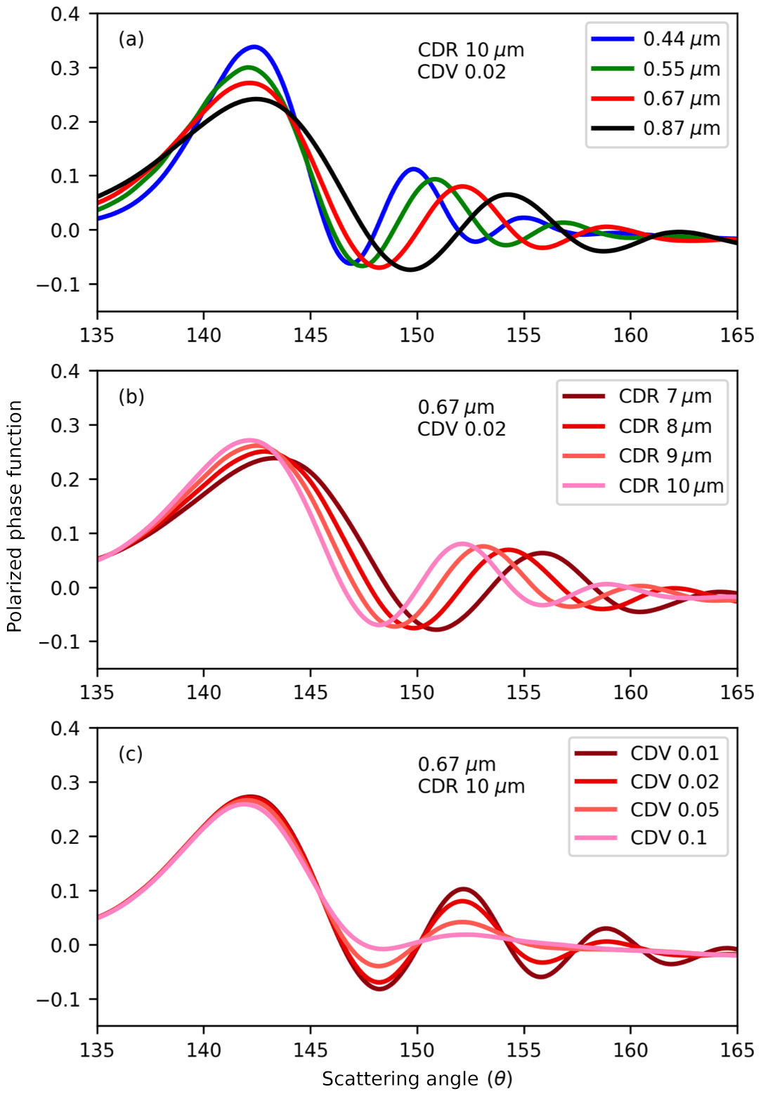
Figure 1 Mie scattering simulations for liquid water cloud droplets, with solar light incident, for the four HARP wavelengths at 10 µm CDR and 0.02 CDV (a), the 0.67 µm channel for variable CDR and constant CDV (b), and constant CDR with variable CDV (c).

Not all polarimetric measurements will achieve a high-quality retrieval of cloud DSDs. Multi-angle sampling at high angular density and moderate pixel resolution is an essential element of an accurate single-wavelength retrieval. Figure 1 shows theoretical Mie simulations that mimic the polarized cloudbow for particular values of CDR, CDV, and wavelength. To resolve the cloudbow patterns from space and retrieve the CDR and CDV of the cloud, the multi-angle polarimetric instruments must satisfy a minimum viewing angle density (Miller et al., 2018), which is directly related to scattering angle coverage. The location of the supernumerary peaks in scattering angle encode CDR in the 0.67 µm example shown in Fig. 1. To resolve the CDV, the amplitude of the supernumerary peaks must be detected. Polarimeters with coarser viewing angle separation for a single wavelength (i.e., >3^∘ at 0.67 µm for typical droplets <15 µm; Miller et al., 2018) may not distinguish these cloudbow oscillations. Instruments like POLDER, which samples at 14 unique viewing angles separated by 10^∘, do not provide enough native angular resolution (Shang et al., 2015) and, as a consequence, may not be able to identify wide versus narrow DSD clouds at specific geometries (Miller et al., 2018). Only when sampling all native 6×7 km POLDER pixels inside a 150 km superpixel can they access the full scattering angle coverage in Fig. 1 and perform an accurate retrieval (Breon and Goloub, 1998). However, this limits their retrievals to large-scale, homogenous marine stratocumulus clouds with narrow DSDs. In a study by Breon and Doutriaux-Boucher (2005), a comparison between POLDER polarized and MODIS radiometric retrievals showed a CDR bias of 2 µm that could not be fully decoupled from the large POLDER superpixel. Later evaluation by Alexandrov et al. (2015), with the RSP and the Autonomous Modular Sensor spectrometer, found that the CDR values retrieved by the two methods agree at narrower resolution. Shang et al. (2015) improved the POLDER retrieval by reducing the superpixel to 42 km. Even though sampling at higher resolution produced gaps in cloudbow coverage, they still found heterogeneity inside the original 150 km superpixel using this improved method. In a follow-up paper, Shang et al. (2019) showed that the POLDER retrieval is sensitive to a wider CDR and CDV range and can be done at a lower 40–60 km resolution when considering all three polarized wavelengths (490, 670, and 865 nm) in the retrieval. Even so, no instrument thus far has performed a polarimetric cloud retrieval from space with both co-located pixel resolution less than 40 km and high native angular density (<10^∘). These goals are essential to studying the spatial distribution of DSDs for heterogeneous, broken, and popcorn cumulus cloud scenes other than the conventional retrievals from marine stratocumulus cases.

The benefit of aircraft instruments like RSP, AirMSPI, and AirHARP is to demonstrate new technologies that improve upon the POLDER retrieval heritage. RSP, in particular, samples at 150+ viewing angles, separated on average by ∼0.8^∘, and does so for a co-located 250 m along-track pixel (Alexandrov et al., 2012b, 2015, 2016b). This advancement removes any large-scale homogeneity assumptions and allows for a rainbow Fourier transform on the data, one that retrieves the DSD itself, including multiple modes, without any assumptions on the distribution shape (Alexandrov et al., 2012b). RSP can sample other kinds of clouds, including broken and popcorn cumulus clouds, with high angular and spatial resolution and does so with high polarimetric accuracy (Cairns et al., 1999). The single-pixel cross-track swath of RSP, however, restricts its spatial coverage: RSP cannot form an intuitive image of the scene, requires specific solar angles for cloudbow coverage (Alexandrov et al., 2012b), and requires input from other coincident instruments for off-nadir context (Alexandrov et al., 2016a). Conversely, the AirMSPI instrument is a highly accurate push-broom imager capable of discrete, programmable viewing angles on the same target, but it has the same angular limitations as POLDER in this step-and-stare mode. AirMSPI also samples in a continuous sweep mode that trades co-located information for scattering angle coverage (Diner et al., 2013). This mode gives full visual coverage on the cloudbow but limits the retrieval to a line cut of binned pixels along the solar principal plane. A study by Xu et al. (2018) extended the AirMSPI line-cut retrieval to the entire continuous sweep image of the cloudbow with assistance from image-specific empirical correlations between COT, CDR, and CDV. This line-cut polarimetric technique requires a droplet size homogeneity assumption over the full line cut of the cloudbow, which may blur heterogeneity that exists at the pixel level and steer the retrieval towards wider DSDs.

There is a strong interest in the Earth science community in a multi-angle polarimeter concept for aerosol and cloud retrievals with a wide swath for spatial context, high accuracy in polarization, high angular density for cloudbow retrieval, and narrow ground resolution (Remer et al., 2019; Dubovik et al., 2019). The Earth and Space Institute (ESI) at the University of Maryland, Baltimore County (UMBC), designed, developed, and deployed the Airborne Hyper-Angular Rainbow Polarimeter (AirHARP), a next-generation wide-field-of-view (FOV) imaging polarimeter specifically for this purpose. AirHARP is the aircraft demonstration of spaceborne technology that will fly on a stand-alone CubeSat platform in 2019 in the orbit of the International Space Station and an enhanced HARP sensor for the NASA Plankton–Aerosol–Cloud–ocean Ecosystem (PACE) mission, called HARP2, in the early 2020s.

In this paper, we will first describe the HARP concept and frame the AirHARP instrument and its data as a proxy for upcoming HARP CubeSat and HARP2 space instruments throughout the rest of the work. We then explain the cloud droplet retrieval framework in Sect. 3, followed by applications of the retrieval on a stratocumulus cloud deck observed by AirHARP during the NASA Lake Michigan Ozone Study field campaign in 2017 in Sect. 4. In Sect. 5, we make use of the fine spatial resolution of the retrieved DSD parameters to explore the information content of the retrieval itself and relate the spatial variability of the results to cloud processes. Section 6 discusses the uncertainties and current limitations of the procedure, and we conclude the paper in Sect. 7, looking ahead to HARP CubeSat and HARP2 deployment and data content.

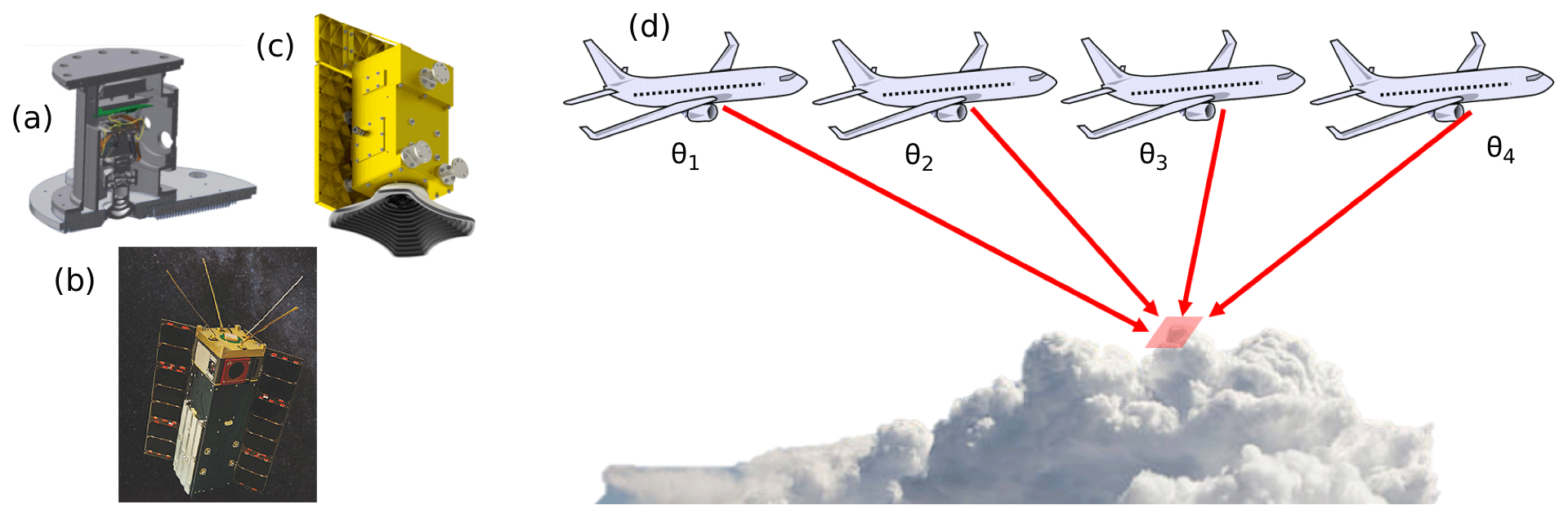
Figure 2 Panels (a), (b), and (c) illustrate the current HARP VNIR polarimeter family consisting of the AirHARP airborne system (a), HARP CubeSat (b), and HARP2 for the NASA PACE mission (c). The HARP concept comprises a wide-field-of-view imaging polarimeter that images the same ground target from up to 60 distinct viewing angles at 0.67 µm (d) and up to 20 viewing angles at 440, 550, and 870 nm. The wide cross-track swath (94^∘) of HARP2 allows for global coverage from space within 2 d.

2 Airborne Hyper-Angular Rainbow Polarimeter

The AirHARP concept, and the HARP family of polarimeters in general, was developed with a wide swath, fine angular resolution, and high polarization accuracy to address some of the limitations of modern polarimeters. The three HARP instruments, shown in Fig. 2, are amplitude-splitting, wide-FOV polarimetric cameras. Incident light enters through the wide-FOV front lens, passes through telecentric optics, and is split by a Phillips prism toward three detectors. Before reaching each detector, this light passes through a polarizer oriented at 0, 45, or 90^∘. The polarizers are oriented at 45^∘ separations such that the I, Q, and U Stokes parameters of the scene can be retrieved in a single co-aligned pixel from an orthogonal basis set of polarization states (Fernandez-Borda et al., 2009). AirHARP images a ground scene with a ±57^∘ (±47^∘) along-track (cross-track) FOV, and a custom stripe filter over the detector assigns 120 along-track portions, or view sectors, of the FOV to four visible channels (bandwidths): 440 (14), 550 (12), 670 (18), and 870 (37) nm. A view sector specifically defines a segment of the detector that corresponds to a unique average viewing angle at the front lens. The hyper-angular 670 nm band samples at 60 view sectors at an average 2^∘ separation, and the other three channels sample at 20 each at an average 6^∘ separation. In this way, the 60 670 nm view sectors can sample the cloudbow oscillations at high angular density without large-scale homogeneity assumptions or degrading the measurement for scattering angle coverage. The wide FOV also allows for broad scattering angle coverage from space during the daylit portion of an orbit. The 20 view sectors in the other three channels ensure multi-angle coverage on aerosols; several studies show that fewer than seven unique views in a single channel are appropriate for high-accuracy retrieval of aerosol optical properties (Hasekamp and Landgraf, 2007; Hasekamp et al., 2019), though the details are beyond the scope of this paper. AirHARP is a push-broom imager, meaning that consecutive measurements from a single view sector can be stitched together to form an image of a ground scene as observed only from that angle. These push brooms can have any along-track length but a cross-track swath proportional to the flight altitude multiplied by a factor of 2.14. This factor accounts for the maximum AirHARP cross-track view angle, ±47^∘. A unique push broom is made for each of the 120 view sectors, and post-processing registers all of them to a common grid.

A target, either on the ground or in the atmosphere, will be viewed from a subset of the 120 view sectors with its reflected apparent I, Q, and U measured in each view sector and wavelength. From these measurements, the polarized reflectance as a function of scattering angle can be compared with theoretical Mie calculations, as in Fig. 1. The hyper-angular capability of the 670 nm channel with its 2^∘ viewing angle resolution can best measure the supernumerary location and amplitude of the cloudbow structure and is therefore best for retrieving the CDR and CDV of the target cloud. Note that because AirHARP is an imager, each pixel in the image is a potential target viewed by multiple angles. Therefore, each pixel in the image can produce its own polarized reflectance and can be used to retrieve CDR and CDV, granted that the range of view angles spans a sufficient range of scattering angles. Note that the scattering angle range is dependent on both the view angle range (fixed by the instrument) and solar geometry (not fixed). If a large number of pixels in the image are viewed at the correct geometry then a spatial map can be made of the DSD parameters across and along the swath, wherever a cloud pixel is found. Depending on the observation altitude and binning scheme, ∼0.2 to 6 km native retrieval resolutions are possible. Therefore, the microphysics of individual fair-weather cumulus clouds can be retrieved across a cloud field stretching tens to hundreds of kilometers. This capability is unprecedented for any existing multi-angle polarimeter instrument.

In HARP's current configuration, all of this retrieval potential fits entirely inside a $\mathrm{10}\times \mathrm{10}\times \mathrm{15}$ cm enclosure. The flagship version of HARP is a spaceborne CubeSat, a stand-alone payload funded by NASA's Earth Science Technology Office (ESTO) In-space Validation of Earth Science Technologies (InVEST) and in collaboration with the Space Dynamics Laboratory (SDL) in Logan, Utah, USA. The HARP CubeSat satellite was launched on 2 November 2019 to the International Space Station (ISS) (400 km, 51.6^∘ inclined orbit) and then dispatched from the station for an autonomous year-long mission in February 2020. Cloud retrievals on HARP CubeSat data will be possible at a minimum 4 km superpixel, a capability demonstrated in this paper using AirHARP, a near-identical copy of the CubeSat instrument for aircraft. A third HARP concept, HARP2, is currently under development for the PACE mission to launch in the early 2020s. The HARP CubeSat will be the first satellite to perform wide-swath polarized cloud retrievals at sub-5 km co-located resolution from space, and HARP2 will continue this capability forward and expand it to provide global coverage in 2 d.

The remainder of this paper will discuss the information content retrieved from complex cloud scenes observed by AirHARP. The study below refers specifically to AirHARP datasets, but the HARP term may be used when discussing general performance expected from any of the HARP instruments.

3 Retrieval framework

A simple treatment of the parametric retrieval is described below, with main components derived from Breon and Goloub (1998), Alexandrov et al. (2015), and Diner et al. (2013). The interaction between incident light and a liquid water cloud droplet is described by a scattering matrix:

$$\begin{array}{}\text{(1)}& {\left[\begin{array}{l}I\\ Q\\ U\end{array}\right]}_{\mathrm{sca}}={\displaystyle \frac{{\mathit{\sigma }}_{\mathrm{sca}}}{\mathrm{4}\mathit{\pi }{R}^{\mathrm{2}}}}\left[\begin{array}{ccc}{P}_{\mathrm{11}}& P_{\mathrm{12}}& \mathrm{0}\\ P_{\mathrm{12}}& P_{\mathrm{22}}& \mathrm{0}\\ \mathrm{0}& \mathrm{0}& P_{\mathrm{33}}\end{array}\right]{\left[\begin{array}{l}I\\ Q\\ U\end{array}\right]}_{\mathrm{inc}},\end{array}$$

where a Stokes column vector describes the incident beam (subscript “inc”), in total radiance (I) and polarized radiance (Q, U), and the scattered beam by a similar vector with subscript “sca”. In general, 16 elements describe the scattering matrix, but since circular polarization in the atmosphere is negligible (Cronin and Marshall, 2011) and not measured by AirHARP, the fourth column and row are neglected. Cloud-top liquid water droplets are spherical, randomly oriented, and mirror symmetric: any matrix elements in Eq. (1) that describe asymmetry are neglected and the others mirror across the main diagonal (Hansen and Travis, 1974). The unitless P_mn matrix elements scale by the droplet scattering cross section (σ_sca) weighted by the inverse of droplet surface area.

Sunlight incident on the atmosphere is unpolarized ($Q_{\mathrm{inc}},U_{\mathrm{inc}}=\mathrm{0}$). For single-scattered photons, the scattered intensity (I_sca) is proportional to the first matrix element, P₁₁ and its polarization (Q_sca) to the second, P₁₂, called the polarized phase function. U_sca does not contain any structural information in the scattering plane, though it may show a weak linear slope in the presence of non-cloud scatterers (Alexandrov et al., 2012a). For this reason, Q_sca in the scattering plane represents the entire polarized signal.

At the top of the atmosphere (TOA), remote sensors do not observe the scattering from individual droplets but the bulk behavior of the droplet distributions due to measurement resolution and scale limitations. The bulk Mie polarized phase function, 〈P₁₂〉, is a weighed sum of optical properties:

$$\begin{array}{}\text{(2)}& \begin{array}{rl}& \langle P_{\mathrm{12}}(\mathit{\lambda },\mathit{\theta },\text{CDR},\text{CDV})\rangle \\ & ={\displaystyle \frac{\sum _i{P}_{\mathrm{12},i}\left(\mathit{\lambda },\mathit{\theta },\text{CDR},\text{CDV}\right){\mathit{\omega }}_i\left(\mathit{\lambda }\right)C_{\mathrm{ext},i}\left(\mathit{\lambda }\right)}{\sum _i{\mathit{\omega }}_i\left(\mathit{\lambda }\right)C_{\mathrm{ext},i}\left(\mathit{\lambda }\right)}},\end{array}\end{array}$$

where ω is the single-scattering albedo (SSA, 1 for water droplets), and C_ext is the scattering cross section, which itself is composed of the scattering efficiency and a size distribution weighted by droplet cross section. This study uses the same unimodal gamma size distribution function as Breon and Goloub (1998). Polarized reflectance observed at TOA from liquid water cloud droplets is proportional to P₁₂, after a correction for viewing geometry:

$$\begin{array}{}\text{(3)}& {\mathcal{R}}_{\mathrm{obs}}={\displaystyle \frac{\mathrm{4}}{\mathit{\pi }}}\left({\mathit{\mu }}_{\mathrm{0}}+\mathit{\mu }\right)\left[{\displaystyle \frac{-\mathit{\pi }{Q}_{\mathrm{sca}}}{{\mathit{\mu }}_{\mathrm{0}}{F}_{\mathrm{0}}}}\right],\end{array}$$

where the cosines of the view zenith angle (μ₀) and solar zenith angle (μ) and the band-weighted extraterrestrial solar irradiance (F₀) rescale the polarized radiance (Q_sca). The bracketed term is the polarized reflectance (ρ_P), and a similar expression gives the total reflectance (ρ) using the Stokes parameter I_sca in place of −Q_sca. Subsequent figures use L_670 nm for I_sca and L_P,670 nm for Q_sca radiances, where applicable, and anytime the term intensity is used, it corresponds to a radiance measurement, not reflectance, unless explicitly noted. Because we are only using a single wavelength in our retrieval, radiance and reflectance are interchangeable in terms of the information content shown in the figures. Corrections to Eq. (3) for Rayleigh scattering at observation height are performed in prior studies (Breon and Goloub, 1998; Diner et al., 2013), but the necessity is disputed (Alexandrov et al., 2015): this study accounts for Rayleigh effects in a weak cosine term described below.

The retrieval compares Eq. (3) to a parametric model and infers the CDR and CDV from the best-fitting P₁₂ simulations:

$$\begin{array}{}\text{(4)}& \begin{array}{rl}{\mathcal{R}}_{\mathrm{fit}}\left(\mathit{\lambda },{\mathit{\vartheta }}_{\mathrm{scat}}\right)& =\mathit{\alpha }{P}_{\mathrm{12}}\left(\mathit{\lambda },{\mathit{\vartheta }}_{\mathrm{scat}},\text{CDR},\text{CDV}\right)\\ & +\mathit{\beta }{\cos }^{\mathrm{2}}{\mathit{\vartheta }}_{\mathrm{scat}}+\mathit{\gamma }.\end{array}\end{array}$$

The parametric fit scales the theory, Eq. (4), to observations, Eq. (3), inside the polarized cloudbow scattering angle range (135^∘ $<{\mathit{\vartheta }}_{\mathrm{scat}}>\mathrm{165}$^∘; Di Noia et al., 2019; Shang et al., 2015) with three free parameters (α, β, γ). Corrective factors for aerosol above cloud, cirrus, sun glint, molecular scattering, and surface reflectance signals comprise weak functions of scattering angle (Diner et al., 2013; Alexandrov et al., 2015). The parameter α is related to cloud fraction (Breon and Goloub, 1998) and is therefore accounted for by Eq. (4).

A prescribed lookup table (LUT) in CDR and CDV drives the parametric fit, ranging between 5 and 20 µm in CDR (Δ=0.5 µm), and CDV values of 0.004 to 0.3 at variable intervals, similar to Alexandrov et al. (2015), with Δ values indicating the step size. The LUT is dense for CDV<0.1: the majority of supernumerary bow sensitivity exists below this level and is considerably reduced for CDV>0.1, as shown in Fig. 1. Polarized reflectance measurements are corrected via Eq. (3) and fit in a nonlinear least-squares process to Eq. (4), checking all possible combinations of CDR and CDV in the LUT. The root mean square error (RMSE) and reduced chi-square statistic ${\mathit{\chi }}_{\mathrm{red}}^{\mathrm{2}}$ of the least-squares process verify all LUT comparisons:

$$\begin{array}{}\text{(5)}& \text{RMSE}=\sqrt{{\displaystyle \frac{\mathrm{1}}{n}}{\sum }_i^n{\left({\mathcal{R}}_{\mathrm{fit},i}-{\mathcal{R}}_{\mathrm{obs},i}\right)}^{\mathrm{2}}},\end{array}$$

and

$$\begin{array}{}\text{(6)}& {\mathit{\chi }}_{\mathrm{red}}^{\mathrm{2}}={\displaystyle \frac{\mathrm{1}}{n-\mathrm{5}}}{\sum }_i^n{\displaystyle \frac{({\mathcal{R}}_{\mathrm{fit},i}-{\mathcal{R}}_{\mathrm{obs},i}{)}^{\mathrm{2}}}{{{\mathit{\sigma }}_{\mathrm{obs},i}}^{\mathrm{2}}}}.\end{array}$$

The ${\mathit{\chi }}_{\mathrm{red}}^{\mathrm{2}}$ verifies that the data are best described by the fit in Eq. (4) with n−5 degrees of freedom (for three fit parameters, CDR, and CDV), where n is the number of measurements in the cloudbow scattering angle range for that pixel. Like Alexandrov et al. (2015), a fine-scale interpolation is performed on the LUT at 10 times the original resolution in CDR and CDV. Retrievals are accepted immediately for ${\mathit{\chi }}_{\mathrm{red}}^{\mathrm{2}}$ values 0.5 to 1.5. In this range, our error estimate is consistent with the minimized fit. If the ${\mathit{\chi }}_{\mathrm{red}}^{\mathrm{2}}$is outside this range, our error may lead to an overfit (${\mathit{\chi }}_{\mathrm{red}}^{\mathrm{2}}<\mathrm{0.5}$) or underfit (${\mathit{\chi }}_{\mathrm{red}}^{\mathrm{2}}>\mathrm{1.5}$). However, large ${\mathit{\chi }}_{\mathrm{red}}^{\mathrm{2}}$ does not always mean the fit is poor in our case: the physics of the cloud field may justify solutions with ${\mathit{\chi }}_{\mathrm{red}}^{\mathrm{2}}$ beyond 1.5. Therefore, we also check to see if the fit satisfies an RMSE threshold of 0.03. If not, the fit is rejected and the pixel is flagged. These diagnostics were found by a sensitivity study on synthetic AirHARP cloudbow retrievals and an estimation of the error in the actual data.

There are several reasons for this two-factor authentication. First, we recognize that the signal-to-noise ratio of the superpixel is not the only error that contributes to the measurement. Optical etaloning (andor.oxorinst.com, 2020) that remains in this AirHARP dataset will also add uncertainty. This effect is weak compared to the signal and nearly random angle to angle, so we estimate an extra 1σ contribution in each superpixel to account for it. Therefore, the superpixel uncertainty, σ_obs, used in Eq. (6) represents 2 times the standard deviation of the superpixel bin. Because the ${\mathit{\chi }}_{\mathrm{red}}^{\mathrm{2}}$ value depends heavily on a correct error estimation, it is important that all artifacts in the data are well accounted for. Second, there is evidence in the literature that when multiple DSDs exist inside the same superpixel, the polarized signal will not agree completely with a signal that represents a single DSD (Shang et al., 2015). This retrieval will still attempt to find a representative DSD in the measurement, however. Here, the ${\mathit{\chi }}_{\mathrm{red}}^{\mathrm{2}}$ may be higher than 1.5, but the RMSE threshold can still find a solution if the measurement residuals are not too far from the best-fit curve. This may also occur for observations of multi-layer cloud fields. Because the ${\mathit{\chi }}_{\mathrm{red}}^{\mathrm{2}}$ depends strongly on the uncertainty of the individual measurements, there is also a possibility that pixels that represent narrow size distributions may give a valid retrieval, while producing ${\mathit{\chi }}_{\mathrm{red}}^{\mathrm{2}}$ values beyond 1.5. Figure 6a is one such example. The cloudbow oscillations are well-defined and AirHARP data clearly capture the pattern, though the ${\mathit{\chi }}_{\mathrm{red}}^{\mathrm{2}}$ is 2.52. While the error bar on several AirHARP data points does not touch the best-fit polarized reflectance, the overall curve fit does represent the information content in the measurement. It is therefore important to include the RMSE as a two-factor authentication. Third, Breon and Goloub (1998) noted that secondary and tertiary scattering events in the primary bow region (137–145^∘ in scattering angle) can widen the polarized signal here relative to Mie simulations. Here, the RMSE may preserve a strong fit in the supernumerary region, where the majority of the DSD information content lies, even if the ${\mathit{\chi }}_{\mathrm{red}}^{\mathrm{2}}$ is beyond our threshold. These diagnostics also account for any artifacts that arise from rotating our reference frame of polarization into the scattering plane and retrievals that converge artificially to the edges of the LUT. When the uncertainty is high relative to the measurement, both ${\mathit{\chi }}_{\mathrm{red}}^{\mathrm{2}}$ and RMSE will also be high and the retrieval will be rejected if both values exceed their expected ranges. More details on some of these effects are discussed in Sect. 6.

The focus of this paper is on the application of AirHARP cloud datasets and not the retrieval algorithm itself; therefore, we use a simple treatment of the classic parametric model. This retrieval will be extended to multi-modal DSDs and take into account both multi-angle and multi-spectral sampling in future studies.

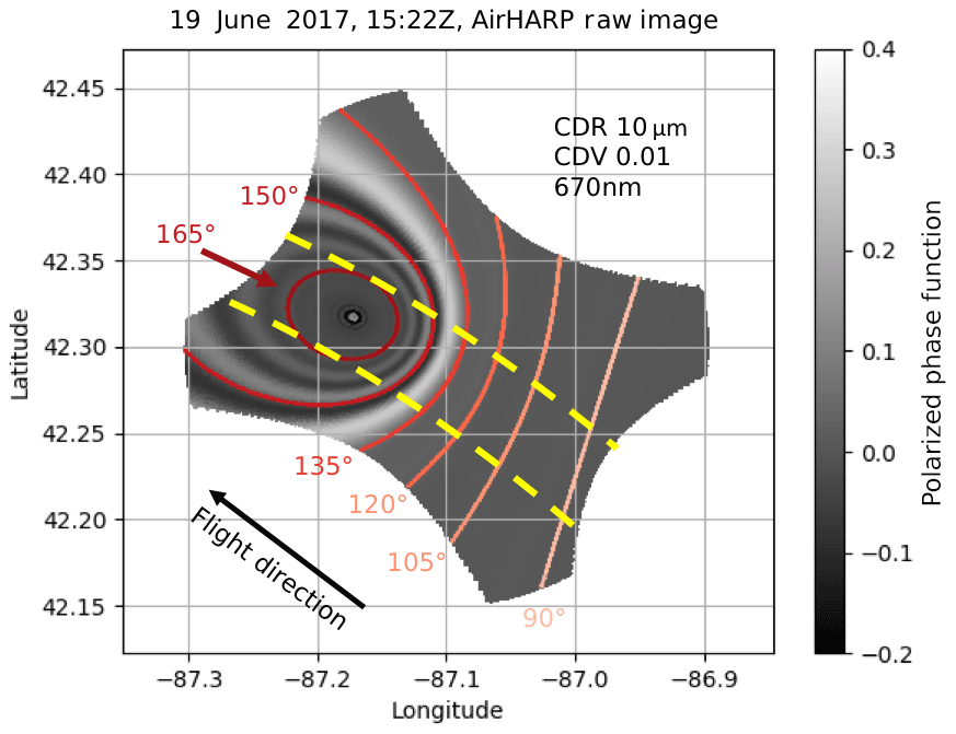
Figure 3 The scattering angle coverage typical of an instantaneous AirHARP wide-FOV observation, projected to simulate a scene over Lake Michigan on 19 June 2017 at 15:22 Z (a). The cloudbow in this simulation represents a simulated cloudbow at 670 nm, with CDR 10um and CDV 0.01, with scattering angle isolines from 90 to 165^∘ shown (solid lines). Note that the cloudbow pattern occurs within 135–165^∘ in scattering angle, and the location of the cloudbow in the FOV depends on time of day, flight orientation, and solar geometry. Note that the only portion of the image that is eligible for retrieval lies inside the region defined by along-track lines tangent to the 165^∘ scattering angle isoline (yellow dotted lines).

4 Hyper-angular polarized cloud retrievals from AirHARP

Before we discuss how the retrieval is applied to the AirHARP data, we will first walk through an AirHARP measurement. As the AirHARP instrument images a scene for a particular solar geometry, each view sector captures a range of scattering angles unique to each of the 120 view sectors and wavelengths. Figure 3 shows an example of the AirHARP instantaneous scattering angle coverage for a simulated observation at 15:22 UTC over Lake Michigan on 19 June 2017 during the NASA Lake Michigan Ozone Study (LMOS) field campaign. This target was chosen because of the cloud conditions present during the observation, and the solar geometry allows for retrievals across the swath and along the entire length of the observation. Figure 3 shows a simulated cloudbow as it would appear in a single AirHARP snapshot if the entire detector was capable of sampling at 670 nm. This cloud field was simulated using a CDR of 10 µm and CDV of 0.01, with the same solar and viewing geometry of the LMOS observation. Note that this is the scattering angle coverage for a single snapshot, and when AirHARP flies over a cloud deck, it is taking two snapshots a second. This means a different portion of the detector is imaging the same cloud target from image to image, which also suggests that the scattering angle observed at the target changes image to image as well. From the perspective of the detector, the target travels from the front of the detector to the back during a full angle observation, reflecting solar light at different scattering angles as the instrument flies over it. Therefore, only along-track pixel columns inside the yellow dotted lines in Fig. 3 contain pixels that are eligible for a polarimetric DSD retrieval. This work does not perform a retrieval on any targets observed outside these lines. Outside these lines, the reduced scattering angle coverage at the upper end of the cloudbow range begins to truncate the signal from the supernumerary bows. Because the majority of the size distribution information is encoded in the supernumerary bows (145–165^∘), it is important that the full scattering angle range is preserved.

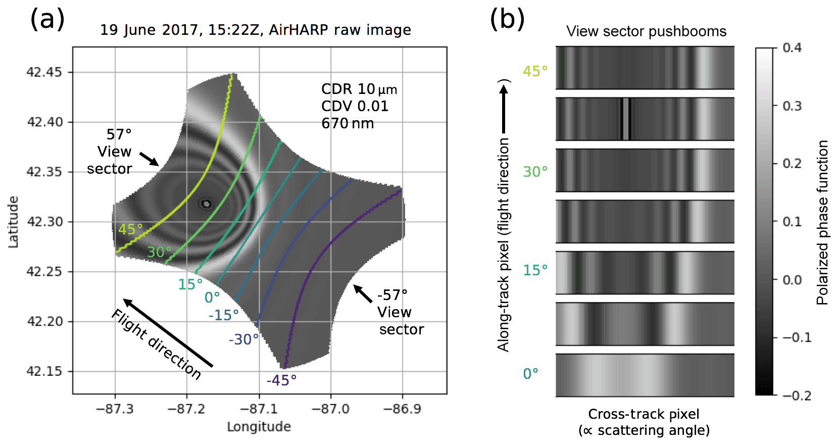
Figure 4 The same simulation as Fig. 3, now with along-track view sector (zenith angle) isolines (a). A push broom is made when a view sector images consecutive information along-track, shown for seven view sectors, separated by 7.5^∘ each (b). Because cross-track pixels represent a cross section of the cloudbow, they are also proxies for scattering angle. Note that the cloudbow distribution is different for each view sector push broom. Since each push broom is projected on a common grid, any pixel or superpixel in common to all of the views can generate a discrete polarized structure. This measurement can be compared to Mie simulations to retrieve CDR and CDV at the target resolution.

Figure 4 shows the view sector isolines of AirHARP over the same snapshot from Fig. 3. The AirHARP wide FOV covers view sectors from ±57^∘, but note that the cloudbow only covers a subset of these. Push brooms are made from individual view sectors as the instrument flies over the cloud field. Figure 4b shows examples of push brooms built from cloudbow content in Fig. 4a isolines. If AirHARP was to fly over this simulated field, the cloudbow would transition from a concentric space in the raw image to a linear one in the push brooms. This occurs because each view sector only observes a specific cross section of the cloudbow at any one time, and the structure of the cross section is maintained due to the geometry of a single view sector. Figure 5 shows the actual AirHARP observation during LMOS, in total (top) and polarized reflectance (bottom), at view sectors near +38^∘ during the time and day used to simulate Figs. 3 and 4. The red–green–blue (RGB) composite image of the polarized reflectance displays the cross-track cloudbow structure of the segment near +38^∘ in the Fig. 4b simulation. The polarized reflectance image shows the wavelength dependence in the polarized cloudbow structure, which is absent from the total reflectance image. Also, the appearance of the cloudbow in this push broom is highly variable compared to the simulation in Figs. 3 and 4, which reflects the heterogeneity in the cloud field seen in total reflectance.

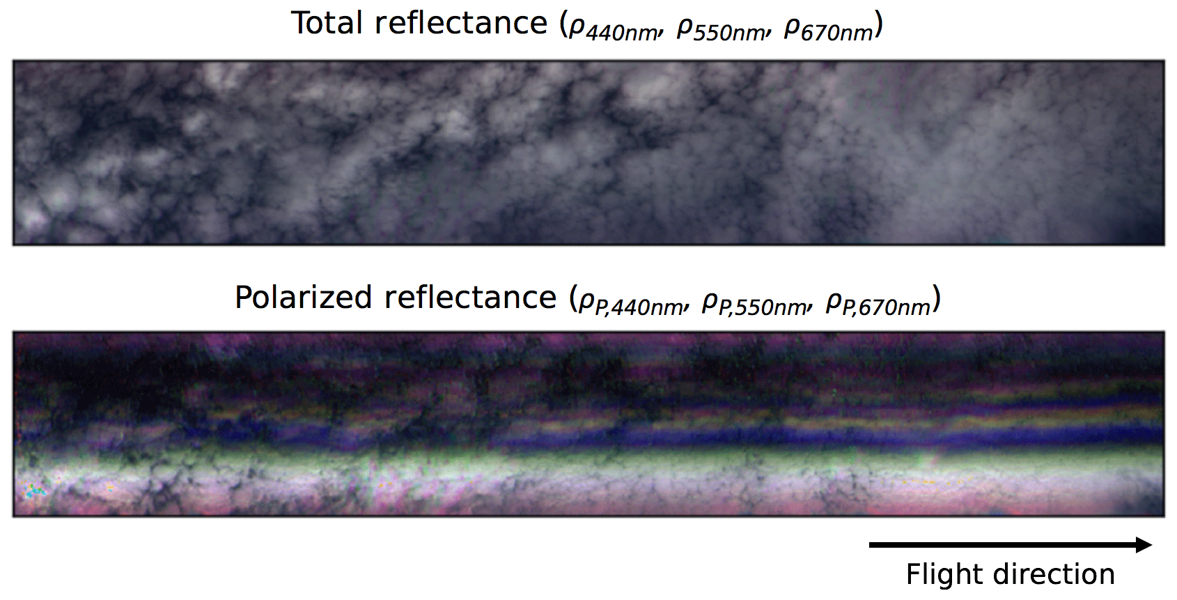
Figure 5 AirHARP data taken at the same time, location, and geometry as Figs. 3 and 4 reveal a heterogenous cloud field in total reflectance (a) and a cloudbow in polarized reflectance (b). The linear distribution of cloudbow oscillations is heterogenous compared to the Fig. 4b simulation and reflects the variability in the cloud field. Both images are RGB composites of push brooms from 440, 550, and 670 nm view sectors near +38^∘, presented without axes for visual purposes only. A single gridded pixel in this image represents 50 m, and the scene stretches approximately 37 km along-track by 5 km cross-track.

Since a single target moves across the detector in consecutive snapshots, there will always be a location in each of the 120 push brooms that represents that target on the ground, and any cloudbow target appearing in multiple sector views having sufficient scattering angle range can be used in a polarimetric cloud DSD retrieval. Figure 6 shows several examples of an AirHARP 200 m superpixel retrieval of different regions of the LMOS cloud field shown in Fig. 5 using hyper-angular, co-located information. Error bars represent 2 times the standard deviation of the polarized reflectance measured by the pixels inside the superpixel bin. Superpixels are constructed from finer-resolution native pixels to increase SNR and mitigate other potential artifacts in the data. These artifacts will be discussed in Sect. 6. Note that Fig. 6a and b both represent narrow DSDs with low CDV values, though the difference in CDR causes a shift in the location of the observed supernumerary bows. Figure 6c and d are wider DSDs with higher CDV values, with eroded supernumeraries. As the DSDs become wider and wider, this retrieval method becomes less and less accurate at inferring CDV, as the supernumerary region becomes monotonic and linear. The CDR values retrieved in Fig. 6 are typical of non-precipitating stratocumulus cloud fields (Pawlowska et al., 2006), and CDV values are similar to those found by Alexandrov et al. (2015) using RSP measurements over marine stratocumulus.

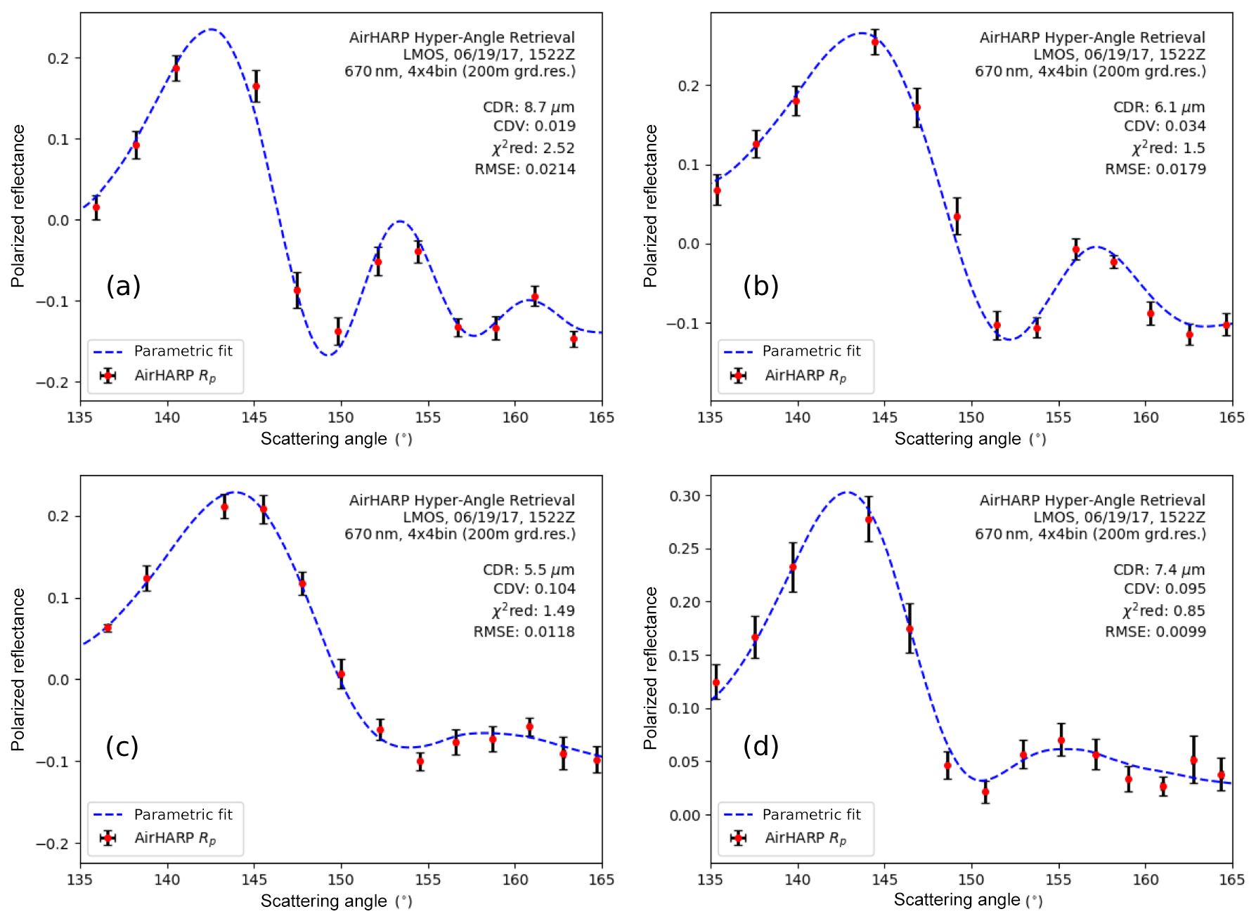
Figure 6 Several examples of the traditional parametric fit retrieval applied to AirHARP hyper-angular polarized reflectance measurements for 200 m superpixels. Panels (a) and (b) signify narrow DSDs with small CDV values. In panels (c) and (d), the eroded supernumerary bows suggest wider DSDs. Error bars represent the 2σ standard deviation of the measurements inside the superpixel. Note that while the ${\mathit{\chi }}_{\mathrm{red}}^{\mathrm{2}}$ in (a) is larger than our 1.5 threshold, the overall fit to measurement generates a valid RMSE.

The hyper-angular retrieval requires data that are captured over a short time window as AirHARP flies over a cloud: it takes time for the AirHARP backward angles to image the same location on the ground as the forward angles. The differences in time depend on the instrument-level flight speed and the difference in altitude between the instrument and target. For the LMOS campaign, the difference between ±57^∘ observations was 112 s (∼2 min) for a nominal UC-12 flight speed of 133 m s⁻¹ at 4.85 km of altitude above the cloud deck. Note that the actual aboveground altitude was 8 km, but the cloud deck was geolocated to be 3150 m on average. Therefore, the hyper-angular retrieval requires cloud constancy over this time interval. If we only include the angles used in the cloudbow retrieval, the time interval between the views with the largest angular separation is reduced to a minute. A study with the HARP CubeSat at an estimated 400 km orbital altitude and 7.66 km s⁻¹ ISS speed requires ∼160 s (∼2.5 min) for the same full-angular coverage over the same cloud target. In this way, the HARP hyper-angular retrieval still requires an assumption of homogeneity in a short time window over a narrow pixel.

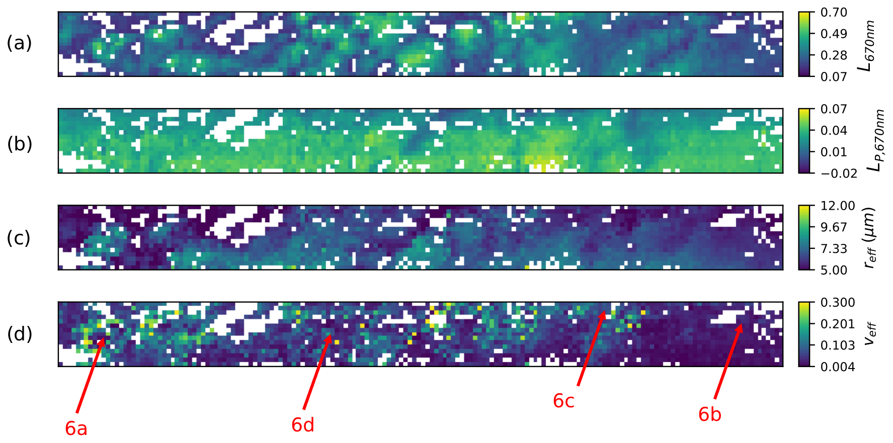
Figure 7 Nadir push-broom images for 670 nm of total intensity (a) and polarized intensity (b), as well as for the retrieved CDR (c) and CDV (d) for 200 m (4×4) gridded superpixels with access to 135–165^∘ in scattering angle using hyper-angular co-located data. Quality-flagged retrievals are screened out (white). Note that the polarized reflectance is smoother compared with the reflectance image, and both represent nadir (−0.003^∘) view sector push brooms. The general locations of each retrieval from Fig. 6 are identified in red. The scene stretches 3 km cross-track and 34 km along-track.

With this in mind, any liquid water cloud pixel in the AirHARP wide FOV that samples scattering angles between 135 and 165^∘ can be used to retrieve CDR and CDV. This constraint is used in several other polarimetric studies, though with a slight discrepancy on the start of the lower bound (Di Noia et al., 2019; Alexandrov et al., 2015). Shang et al. (2015) found that using a 137–165^∘ scattering angle range as opposed to the operational POLDER 145–165^∘ improved many of the CDR and CDV retrievals, specifically for CDR>15 µm (Shang et al., 2019). The upper bound of 165^∘ is consistent between studies dating back to Breon and Goloub (1998): the bulk of the microphysical information lies in the supernumerary bows, and the assumption of a structureless U_sca breaks down after this point (Alexandrov et al., 2012a). Figure 7 shows an example of how individual pixel retrievals generate a spatial distribution of CDR and CDV for those that access this cloudbow scattering angle range. Each pixel is first conservatively masked for non-clouds using the nadir 670 nm intensity push broom (−0.003^∘ VZA) using a conservative threshold of 0.06 $\mathrm{W}{\mathrm{m}}^{-\mathrm{2}}{\mathrm{sr}}^{-\mathrm{1}}{\mathrm{nm}}^{-\mathrm{1}}$ to avoid cloud holes and views of Lake Michigan below. All pixels are aggregated to 4×4 resolution (200 m), and the polarized radiances (L_P,670 nm) are converted into polarized reflectances via Eq. (3) before entering the retrieval process. The portion of the image capable of retrieval stretches 34 km along-track and 3 km cross-track.

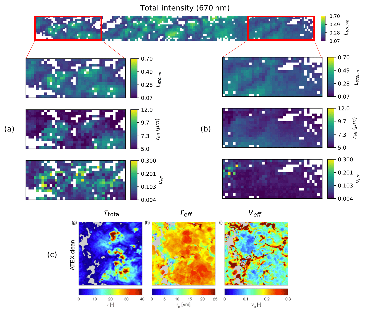
Figure 8 A zoom of two sectors of the AirHARP polarized cloud retrieval for the LMOS cloud field. The intensity image (top) shows both a heterogeneous (a) and a homogenous region (b), defined by the distribution of CDR and CDV, as well as visual cues from the total reflectance. Large-eddy simulations of clean clouds (c), performed by Miller et al. (2018), show that high CDV (v_eff) and low CDR (r_eff) typify cloud periphery regions, and low CDV and higher CDR occur in the core of the clouds. Similar CDV–CDR relationships are seen in the AirHARP retrievals (a) at 200 m resolution.

The distribution of CDR and CDV in AirHARP data is consistent with prior studies and physical phenomena. Because the cloud case observed during LMOS was heterogenous, there are several examples of how cloud substructure can give different retrievals. Figure 8 takes a few areas from Fig. 7 and zooms in on their retrieval results. Figure 8b shows a uniform sector of the cloud field, described this way because of its visual homogeneity in both intensity and CDR as well as the narrow and consistent CDV retrievals over many pixels. The results here suggest that the supernumerary bows are well-defined and the cloud pixels have narrow size distributions. Figure 8a shows a region of the same leg that is heterogeneous in CDV, and the intensity and CDR distribution suggest that this area is a region of convection: larger CDR in the cloud core, or central area of the cloud, and smaller CDR retrieved on the periphery, where the intensity is lower. We will look at this phenomenon in more detail in the AirHARP data in the sections below. Here we point out that large-eddy simulations (LESs) of similar heterogenous clouds show similar spatial distributions of intensity, CDR, and CDV (Miller et al., 2018), with one representative case shown in Fig. 8c. Miller et al. (2018) simulate LES clouds using vertical weighting functions that take into account the distribution of reflectance at the edges of the cloud, echoing theoretical recommendations made by Platnick (2000).

While these simulations can assume any resolution, the AirHARP retrievals are performed at 200 m in this study and even coarser resolutions from space. The small-scale variability in the cloud field can also be missed by MODIS radiometric analyses, for example, which assumes constant CDV in their droplet size retrieval. This is one of the strongest benefits of polarized cloud retrievals: a quantitative measurement of heterogeneity through CDV information, which is not possible with traditional radiometric methods. This has serious implications for climate in terms of quantifying cloud development, brightness, and lifetime, aerosol–cloud interaction, and reducing the uncertainty in global radiative forcing due to clouds and aerosols. In the following section, we explore how we can extend the AirHARP spatial retrievals of CDR and CDV to study changes in size properties along the cloud field and the impact of resolution on the retrieval itself.

Figure 9 Analysis of intensity (blue), CDR (red), and log (CDV) (green) anomalies from the mean following the black transect along the nadir intensity push broom for a segment of the cloud field measured by AirHARP (bottom). Using the spatial distribution of intensity as a proxy for cloud optical thickness (COT), we can visually identify what appear to be cloud cores (blue blocks) and cloud periphery (orange blocks) regions. CDV trends are opposite to intensity and CDR in both regions, but wider DSDs with smaller CDR appear at cloud peripheries, while larger CDRs with narrow DSDs appear in cloud cores. The label X to the left of the intensity image is an abbreviation for cross-track distance from the image center line.

5 Spatial scale analysis

Because the AirHARP retrievals of CDR and CDV are images, any sector of the cloud field can be analyzed by taking a transect of pixels along- or cross-track. In Fig. 9, we take a 34 km pixel transect of the cloud field (shown in the inset intensity image with a black line) and compare the anomaly from the mean along the track for intensity, CDR, and CDV. The CDV is log-scaled to linearize its several orders of magnitude range. Positive CDR anomalies describe larger droplet sizes, and positive CDV anomalies correspond to wider distributions. Any position along the transect of the cloud field lines up exactly with three unique points in the plot, and the correlation between the three curves suggests information about the nature of the cloud field. It is important to note that we are using the cloud intensity as a proxy for COT, which is orthogonal to CDR (Nakajima and King, 1990). In some locations in the plot, intensity (COT) and CDR are correlated with each other and anticorrelated with CDV. Blue blocks define unambiguous locations in the cloud field where intensity and CDR have positive anomalies while the CDV anomaly is negative, whereas orange blocks give the opposite: intensity and CDR are negative and CDV is positive. If we define cloud cores as the pixels brightest in intensity (blue) and cloud peripheries as darkest in intensity (orange) then cloud cell sizes appear to be of the order 1–4 km, both comparable to and slightly larger than traditional MODIS cloud droplet size retrieval products (1 km). Comparison to the traditional cloud product resolution is notable because, in some regards, the 1 km resolution is adequate to resolve cloud microphysics of the cloud cores. However, when cores and peripheries are found in the same 1 km pixel, issues in separating DSDs will arise. Since AirHARP is an aircraft instrument and flies beneath 20 km, its resolution will be better than an equivalent AirHARP instrument in space, so this fine-scale variability will likely not be captured by HARP CubeSat or HARP2. Regardless, this result emphasizes the importance of small-scale sub-kilometer sampling of cloud fields because cloud heterogeneity and microphysical processes may be lost in the large spatial resolutions of spaceborne instruments.

There are physical explanations for the relationships we see between intensity, CDR, and CDV on the spatial scales of Fig. 9. Liquid water droplets that form at the base of adiabatic clouds, such as cumulus and stratocumulus, see their largest sizes at cloud top (Platnick, 2000) and further grow by longwave radiative cooling, small-scale turbulence, and collisional processes (de Lozar and Muessle, 2016). On the periphery, evaporation removes smaller droplets, and at the same time, the entrainment of warm air and/or aerosol here may enhance droplet growth. There are many competing theories as to the net effect of aerosol entrainment on droplet growth (Small et al., 2009, and references therein), but these two opposing effects may create a larger DSD variance on the periphery. Alexandrov et al. (2015) and Platnick (2000) suggest that CDR changes occur vertically in the cloud periphery. Therefore, multi-angle polarimeters that can sample deeper into the periphery could retrieve a larger CDV in these areas. The above LES study of broken marine stratocumulus by Miller et al. (2018) also shows higher CDV (lower CDR) in the cloud periphery and lower CDV (higher CDR) in cloud cores, as shown in Fig. 8c. In the present study, all of these processes cannot be decoupled, but these promising results show that AirHARP retrievals are consistent with current research and theories of cloud microphysics.

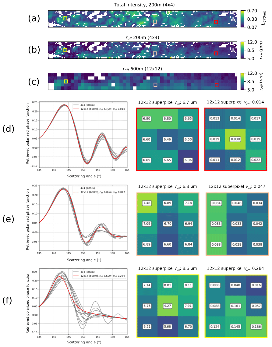
Figure 10 Scale analysis for the scene in Fig. 5 with 200 m (b) and 600 m (c) resolutions. The Mie P₁₂ curves retrieved from the AirHARP data are shown with gray lines in panels (d), (e), and (f), and the direct 600 m superpixel P₁₂ retrieval is shown in red for three difference cases: narrow (d), two-regime (e), and mixed (f) DSDs. The boxes to the right-hand side show CDR and CDV results for each of the nine 200 m pixel retrievals within the outlined 600 m superpixel. Results of the direct retrieval at 600 m resolution are shown on the top of the boxes. The location of each retrieval site is given as corresponding colored blocks in the retrieval image for narrow (red), two-regime (peach), and mixed (yellow). Note that the 600 m retrievals shown in (e) and (f) give wider CDV results than (d), mainly due to competing size properties at the 200 m level.

Furthermore, the AirHARP pixel resolution can be degraded and used to understand the effect of sub-pixel variability on the DSD retrieval itself, as shown in Fig. 10. Figure 10a and b are repeated from Fig. 7a and b, and both represent the 200 m CDR retrieval, while Fig. 10c shows the CDR product at 600 m resolution. To calculate the 600 m product, the gridded polarized reflectance data at the original 50 m resolution are aggregated into 600 m superpixels. Next, the superpixels pass through a screening process: this eliminates low-intensity superpixels that represent cloud holes and marginal situations. Third, the superpixels enter the retrieval process. Thus, Fig. 10c is not a resampling of Fig. 10b but a new retrieval using a different resolution as input. This study does not examine the effect of cloud screening at the different resolutions, only the effect of the degraded resolution using pixels that have been properly identified as clouds at the finer resolution.

The plots on the left-hand side of Fig. 10d–f are the retrieved P₁₂ curves, which emphasize how the nine 200 m retrievals, shown as gray lines, compare to the single 600 m retrieval, which is shown as a red line. The two boxes to the right of each of the retrieved P₁₂ curve plots in Fig. 10d–f represent the retrieved CDR (middle column) and CDV (right column) for the colored superpixel boxes located in Fig. 10a–c. The 600 m CDR or CDV result is given in the title above each box and represents the retrieval for the entire nine-box square underneath, whereas the 200 m CDR or CDV results are shown inside each colored sub-box.

Figure 10d shows that the narrow DSD retrievals are robust against resolution degradation; if we take the 200 m retrievals as truth, the 600 m result agrees within community standards (10 % σ_CDR and 50 % σ_CDV; Mishchenko et al., 2004). The 600 m P₁₂ resembles the 200 m P₁₂ curves, both in the location of supernumerary peaks and overall structure. Figure 10e shows a retrieval that appears to represent the cloud periphery, as the intensity image shows the appearance of a cloud cell near the superpixel. Here, the CDR retrieval gives higher values in the center of the structure and smaller values on the sides, consistent with prior studies. Figure 10e shows two conflicting P₁₂ regimes. Here, 200 m DSDs with CDR between 6.6 and 7.5 µm separate into two modes: CDV>0.08 and CDV between 0.048 and 0.028. While the primary bow around 143^∘ is preserved between retrieval scales, the 600 m retrieval gives a CDV of 0.047, a value that appears to represent the mean of the nine pixels but satisfies neither regime. Shang et al. (2015) and Miller et al. (2018) show similar results in theoretical and observational mixed DSDs. Note that the combination of gamma distributions inside a superpixel is not itself a gamma distribution, though retrievals that contain sub-pixel heterogeneity in the DSD still attempt to infer gamma distribution properties from a signal that may not represent one (Shang et al., 2015). The rainbow Fourier transform method (Alexandrov et al., 2012b) may distinguish these two modes at the 600 m scale, but the result could not be independently validated if it was performed with RSP single-pixel sampling, as it is here with AirHARP data. Figure 10f shows another retrieval done close to the cloud periphery, but this time, the retrieved 200 m P₁₂ curves show a wider spread of CDV values compared to the results shown in Fig. 10d–e.The retrieved 600 m fit generates a curve that does not represent any of the sub-pixel results. The consequence is a broad 600 m CDV that reflects the 200 m variability but not the mean magnitude of the nine sub-pixels, as the 600 m retrieved value for CDV is 0.284, while the nine individual pixels return values 0.086 to 0.186. Here, the sub-pixel variability smears out the supernumerary bows. This result is a well-known consequence of mixed DSDs in a large superpixel, but it does not provide any information as to which parts of the cloud inside the superpixel contain narrow vs. wider DSDs. The interpretation of CDR and CDV at large pixel sizes is still widely debated, but fine-resolution spatial data provided by AirHARP and its retrievals can provide a meaningful advancement in this direction.

6 Discussion of limitations and uncertainty

The first limitation of this method concerns the parametric retrieval, which assumes a single-mode DSD that can be described by CDR and CDV alone. Situations that do not fit this assumption may not be retrievable, as mentioned above. We note that other retrieval methods will overcome this limitation. However, for the purposes of this initial demonstration, the assumptions of the parametric retrieval seem to be met by our example.

This being said, we cannot ignore the possibility of optically thin upper-level clouds (τ_cld<1) moving over the geolocated cloud deck. If these clouds exist, they will appear to “move” from angle to angle, as our current geolocation algorithm, discussed later on, focuses on the layer of clouds that is producing the dominant signal. This also means their impact on the cloud retrieval will change from angle to angle but will likely affect only two or three view sectors at most, with a weak contribution to the measurement. Therefore, this is not expected to significantly contribute to the overall cloudbow fit. All fits shown in this paper lie beneath our successful RMSE threshold, supporting this claim, though other retrieval methods could tease out the signals from both cloud layers when properly geolocated (Alexandrov et al., 2012b, 2016b).

This limitation, the need to map the different angular measurements to a target elevation, is a significant challenge with AirHARP data. If the target were Earth's surface, then a digital elevation map could be used, but clouds appear at a range of altitudes and are not always easily predictable in height, distribution, time, or space. Therefore, an iterative method determines, within a gridded pixel, the altitude that provides zero parallax displacement in the cloud field. We use the location of several distinguished cloud features, as observed from at least two view sectors, to determine the average cloud height of the dataset. Currently, this single cloud height estimate is applied to the entire dataset during the Level 1 geolocation process. Because there is no such thing as a plane-parallel cloud, both the parallax method and the assumption of constant cloud-top height introduces uncertainty in the retrieval. Where possible, the altitude of the scene is verified with heights retrieved from data from other coincident instruments. Conservative cloud identification and binning pixels to 200 m (4×4) resolution further mitigates the error introduced by using this mean height. In the case shown in Fig. 5, the derived height is (3150±50) m, for which the uncertainty is the resolution that guarantees no movement from view sector to view sector. A self-check on the validity of these assumptions is the goodness of fit of each retrieval. In our example, while the RMSE of the cloud field varies, all retrievals shown successfully fit the RMSE threshold defined above. Therefore, we believe errors in our geolocation do not contribute significantly to the results of our study shown at 200 or 600 m resolutions. However, when studying broken or popcorn cumulus clouds, a proper 3D geolocation of the cloud will be required. The HARP science team is currently developing an optimized pixel-level topographic algorithm to mitigate any multi-layer or cloud projection biases in future retrieval studies, as well as other quality assurance corrections beyond the scope of this work.

During an aircraft campaign, it is also important to maintain calibration accuracy in flight as many factors such as temperature, pressure, vibration, and humidification can alter the quality of the measurements. AirHARP did not have an in-flight calibration mechanism during LMOS, so it is challenging to verify the accuracy of the in-flight data. We also realized in lab studies that AirHARP generates internal optical etaloning. The etaloning produces concentric fringes on the raw image, which transform into linear bands at the push-broom level. Typically, a lab flat field corrects for this effect, but our flights show that the etaloning occurs in new locations at the detector during flights. The fringes are variable in strength and size across each view sector but are easily removed over homogenous targets with our current correction scheme. Because the cloudbow also transforms from a concentric to linear space at the push-broom level, cloudbow cases are especially tricky to correct. Luckily, the effect of the fringes on the hyper-angular retrieval is nearly random: the retrieval is a structural fit from angular data that covers many unique positions in the detector. Therefore, the etaloning can be treated as a decrease in SNR in the measurement, which we estimate as an extra 1σ error contribution. Due to the well-resolved retrievals in Figs. 6–10, it is clear that the etaloning does not contribute significantly to the CDR and CDV products, though the fringe contribution would make it more difficult to retrieve above-cloud aerosol signals hidden inside the cloudbow measurement, if applicable. For this reason, we are currently developing a new correction algorithm to remove the fringing from heterogenous datasets and an internal calibrator for HARP2 on the PACE mission. With frequent flat-field calibrations, the etaloning can be immediately corrected in a variety of environments. Also, there is evidence that the cloudbow retrieval itself could be used to remove the fringe signal from AirHARP data. While the cloud signal changes across multiple full-size images, the fringe structure is stable for the same view sector. This allows for the characterization and removal of the fringes uniquely from cloudbow datasets. This is a promising correction technique that will be explored in future work.

Finally, the results of the retrieval presented in this paper are challenging to validate and even difficult to compare with other retrievals. The MODIS Terra and Suomi-NPP VIIRS radiometers passed over the same location on the ground as our example over an hour after the AirHARP observation, and while the GOES-R Advanced Baseline Imager (ABI) radiometer is coincident, its 1–2 km CDR retrieval resolution is difficult to reconcile with the variability observed in the cloud field at finer AirHARP resolution, as suggested by our study presented in Fig. 10. Intercomparing GOES-R and AirHARP retrievals will be performed in a future study; the constant coincidence of GOES-R makes it very attractive for field campaigns that once relied on the sparse coincidence of polar-orbiting or ISS-based sensors. AirHARP was also the only Earth-observing polarimeter present on aircraft or in space during LMOS with these capabilities for cloud retrieval. None of the field experiments in which AirHARP has flown (LMOS or ACEPOL in 2017) focused on clouds, allowing for only a few cloud targets of opportunity during both campaigns. For example, the observation presented in this paper was the only one in which AirHARP achieved full angular coverage over a continuous cloud field and one that could be geolocated to a constant height over the full push broom with little impact to the retrieval itself. A dedicated future aircraft campaign for clouds, specifically one that allows coincident AirHARP observations with other compatible cloud-measuring or -retrieving sensors at similar spatial resolution, would be beneficial for validation. Optimally, coincident HARP space and AirHARP aircraft observations would greatly improve our ability to validate the differences in retrieval resolution for cloud cores and peripheries, across a wide swath, and for unique global locations and aerosol source regions.

7 Conclusion

We used the AirHARP hyper-angular measurements at a single wavelength (670 nm) in a traditional parameterization scheme to demonstrate the ability of the HARP concept to characterize cloud microphysical parameters across a cloud field at sub-kilometer spatial resolution. HARP measurements can also be applied to the four polarized wavelengths, akin to Breon and Goloub (1998) and Shang et al. (2019), but this type of retrieval is more sensitive to resolution and calibration than the hyper-angular technique presented here and most importantly requires homogeneity at cross-track scales (3 km). In the hyper-angular method, we can achieve the same results at the pixel scale (0.2 km) and resolve the spatial inhomogeneity across the track. Variability within a 3 km scale retrieval can easily steer the parametric retrieval towards larger CDV (Fig. 10e; Shang et al., 2015; Miller et al., 2018), and calibration biases that affect an individual view sector (i.e., etaloning) will be much more prominent and systematic in this approach than in the hyper-angle retrieval. Using data from multiple channels (Shang et al., 2019) serves as an excellent cross-calibration and intercomparison with other instruments over narrow DSD marine stratocumulus (Alexandrov et al., 2015; Knobelspiesse et al., 2019), all of which will be explored in future work.

The HARP concept enables highly resolved, hyper-angular polarimetric retrievals of liquid water cloud microphysical properties. Using a heterogenous cloud field from the NASA LMOS campaign as an example, AirHARP datasets allow for sub-kilometer spatial retrievals of CDR and CDV across the full swath and along the entire flight track. These analyses reveal cloud substructure and the spatial distribution of DSDs for cloud cores and periphery regions, which can be easily extended to marine stratocumulus, trade-wind, and popcorn cumulus clouds. Because of the wide HARP FOV, these retrievals are possible off the instrument nadir scan line and during nearly all daytime hours if geometry allows. Combined, these capabilities position HARP as an instrument capable of cloud DSD retrieval at scales relevant to climate study and with global coverage from space.

Because of relatively fine-spatial-resolution retrievals across a broad swath, we were able to perform scale analysis on retrieved DSD parameters by degrading the resolution and subsampling the hyper-angular polarimetric retrieval. At the pixel level, we note that large pixel sizes blur DSD variability, resulting in a retrieval that tries to account for all sub-pixel regimes but ends in producing an entirely different DSD altogether. The sub-kilometer retrievals were able to identify small-scale DSD variability in our heterogenous cloud field. Specifically, we found that there is a correlation between intensity (a proxy for COT) and CDR and an anticorrelation with CDV. For places where intensity is high (high COT), assumed to be cloud cores, droplets were large and size distributions narrow. The opposite is found along the cloud periphery. These findings may be related to entrainment and droplet evaporation on cloud edges and collision–coalescence processes in cloud cores, but further theoretical study and targeted campaigns are needed. Some of these results are not limited to the HARP design: producing spatial images of both DSD parameters can be achieved by other imaging multi-angle polarimeters. Producing these images with a spatial resolution sufficiently fine to illuminate cloud processes along with the spatial coverage to encompass an entire two-dimensional cloud field is unique to the HARP concept.

Future work anticipates extending these concepts to multi-modal size distributions and combining multi-spectral and multi-angle sampling to retrieve cloud size properties and other information: aerosol-above-cloud microphysics, cloud height, and thermodynamic phase, as well as a stronger definition of CDR and CDV for large superpixels that contain internal DSD variability. With the upcoming launch of HARP CubeSat in 2019 and HARP2 in the early 2020s, the same retrieval concepts applied here on AirHARP data can be used to connect cloud properties to global radiative forcing, improve radiometric retrievals, and provide strong science rationale for including high-resolution, hyper-angle imaging polarimetry on future Earth science space missions.