the Creative Commons Attribution 4.0 License.
the Creative Commons Attribution 4.0 License.
 | 08 Apr 2020
Effect of OH emission on the temperature and wind measurements derived from limb-viewing observations of the 1.27 µm O2 dayglow
Weiwei He
Yutao Feng
Yuanhui Xiong
Faquan Li
The O2(a1Δg) emission near 1.27 µm is well-suited for remote sensing of global wind and temperature in near-space by limb-viewing observations to its bright signal and extended altitude coverage. However, vibrational–rotational emission lines of the OH dayglow produced by the hydrogen–ozone reaction () overlap the infrared atmospheric band emission (a1Δg→X3Σg) of O2. The main goal of this paper is to discuss the effect of OH emission on the wind and temperature measurements derived from the 1.27 µm O2 dayglow limb-viewing observations. The O2 dayglow and OH dayglow spectrum over the spectral region and altitude range of interest is calculated by using the line-by-line radiative transfer model and the most recent photochemical model. The method of four-point sampling of the interferogram and sample results of measurement simulations are provided for both O2 dayglow and OH dayglow. It is apparent from the simulations that the presence of OH dayglow as an interfering species decreases the wind and temperature accuracy at all altitudes, but this effect can be reduced considerably by improving OH dayglow knowledge.
- Article
(2604 KB) - Full-text XML
- BibTeX
- EndNote


The infrared atmospheric band emission (a1Δg→X3Σg) of O2 observed near the wavelength of 1.27 µm has remarkable advantages in atmospheric remote sensing due to its bright signal and extended altitude coverage (Mlynczak et al., 2007). The enormous success of the Wind Imaging Interferometer (WINDII) (Shepherd et al., 2012), high-resolution Doppler imager (HRDI) (Ortland et al., 1996) and TIMED Doppler interferometer (TIDI) (Killeen et al., 2006), which measured winds in the upper mesosphere and lower thermosphere using Doppler shifts in visible airglow emission lines, stimulates interest in measuring wind and temperature from limb-viewing satellites using the 1.27 µm dayglow (Wu et al., 2018).
Ward et al. (2001) designed a high-sensitivity interferometer, WAMI, to provide simultaneous measurements of horizontal wind and rotational temperature by using the combination of a “strong” emission line group and a “weak” group of the O2(a1Δg) airglow. A similar instrument, MIMI, designed by York University, also takes advantage of strong and weak emission lines for dynamics and thermodynamics measurement. Both WAMI and MIMI are imaging, field-widened Michelson interferometers and the same measurement technique, known as Doppler Michelson imaging interferometry, is employed successfully by the WINDII instrument on NASA's UARS satellite (Shepherd et al., 2012). The observing strategy of using two sets of three emission lines (as shown in Fig. 1 of Ward et al., 2001) makes it a perfect approach for WAMI and MIMI to improve our knowledge of the wind and temperature of the lower thermosphere and middle atmosphere, as well as global distribution and transport of O3. In recent years, measuring wind and temperature in the planetary atmosphere of Mars and Venus, for example, was also proposed by using a 1.27 µm band emission of the electronically excited O2(a1Δg) state (Ward et al., 2002; Zhang et al., 2017). Closely following the WAMI concept, we recently proposed a near-space wind and temperature sensing interferometer (NWTSI) for simultaneous measurements of the atmospheric wind and temperature in the near-space from the limb-viewing satellite by observing the O2(a1Δg) dayglow near 1.27 µm (He et al., 2019).
The strategy of choosing two sets of three emission lines adopted by WAMI, MIMI and NWTSI is quite ingenious. Three emission lines of each group are relatively well separated and belong to different branches within the same band, which allows them to be optically isolated and ensures distinct temperature sensitivities. Additionally, the line strengths of the strong group and the weak one differ by about 1 order of magnitude, so their radiation intensities and absorption characteristics varying with altitude are available for covering a great extended altitude range from 45 to 100 km.
However, vibrational–rotational emission lines of the OH dayglow produced by the hydrogen–ozone reaction () overlap the infrared atmospheric band emission (a1Δg→X3Σg) of O2 near 1.27 µm (Maihara et al., 1993), which may potentially contribute to the increase in wind and temperature errors.
The main goal of this paper is to discuss the effect of OH emission on the wind and temperature measurements derived from the 1.27 µm O2 dayglow limb-viewing observations. The atmospheric radiance model is simulated using a line-by-line radiative transfer method. A brief description of the O2 dayglow and OH dayglow spectrum over the spectral region and altitude range of interest is provided. The forward simulation including instrument model and the method of four-point sampling of the interferogram, as well as sample results of measurement simulations, is presented. Inversion errors of wind and temperature measurements due to the effect of OH dayglow are presented and discussed. Here we report, to the best of our knowledge, the first consideration and discussion of the effect of OH dayglow on the temperature and wind measurements using the 1.27 µm O2 dayglow.
2.1 The O2(a1Δg) and OH dayglow volume emission rates
Two predominant mechanisms, the photolysis of O3 and the energy transfer from O(1D), produce the lowest-lying electronic state of molecular oxygen O2(a1Δg) in the mesosphere and lower thermosphere. O2(a1Δg) radiates strong emission in the infrared atmospheric band O2(a1Δg)→O2(X3Σg) and produces dayglow at 1.27 µm. The volume emission rate (VER, defined as the number of photons emitted from a cubic centimeter per second) of a O2 individual rotational line can be given by (Mlynczak et al., 1993)
where A is the Einstein coefficient of the transition, g′ is the upper state degeneracy, Q(T) is the rotational partition function, h is the Planck constant, c is the light speed, k is the Boltzmann constant, T is the rotational temperature, E′ is the upper state energy, , , , , , , , , , , , and .
An enhanced concentration of OH• in high states occurs in a thin layer near the mesopause due to the hydrogen–ozone reaction, . A multitude of excited OH* in high vibrational and rotational states cascading to lower energy states results in an emission spectrum, which extends over a wide wavelength range (500–5000 nm). Among those vibrational–rotational transitions, two emission lines, RR2.5e and RR2.5f of the band, are very close to the three weak target emission lines of the 1.27 µm O2 dayglow.
The volume emission rate of the OH (8–5) vibrational band can be given by (Russell and Lowe, 2003)
where [OH(v=8)] is the number density of OH in the v=8 state, is the particular Einstein coefficient for the rotation transition of the (8–5) vibrational band, J′ and J′′ are initial and final values of the total angular momentum of the transition, and is the upper state rotational term value.
Figure 1 shows the VER profiles of both the three weak target emission lines of the 1.27 µm O2 dayglow and the two emission lines, RR2.5e and RR2.5f of the band. As can be seen, the O2 dayglow peaks at about 45 km and the OH reaches 90 km, and the emission rate of O2 is roughly 45 times stronger than OH. In addition, the two emission lines of OH show a similar distribution profile over altitude, while the three emission lines of O2 differ a lot. This is because the two emission lines of OH share the same particular Einstein coefficient and total angular momentum, but the three emission lines of O2 are located in different vibration bands with sufficiently different lower-state energy, which leads to a disparity in temperature sensitivity.
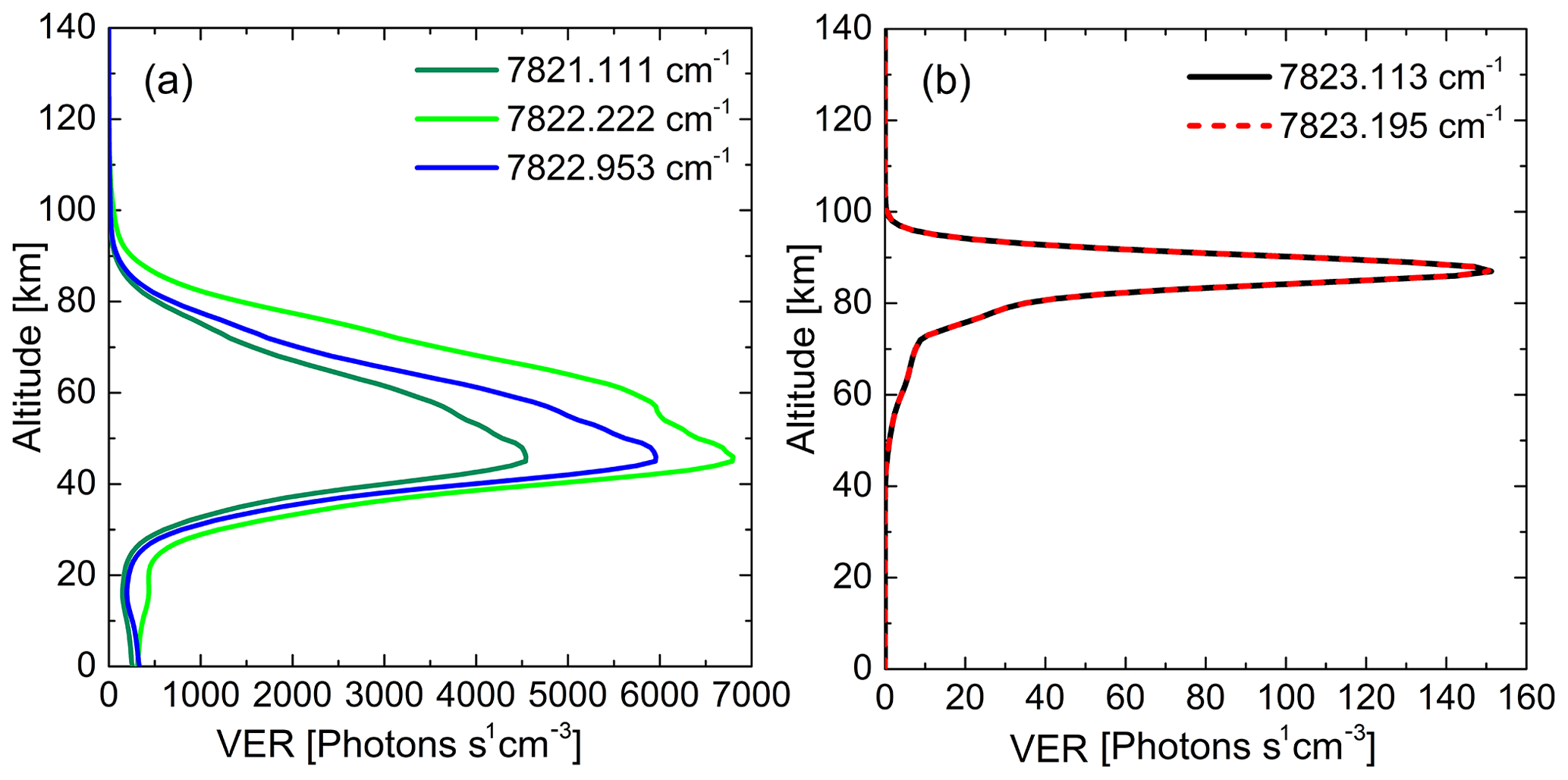
Figure 1The VER profiles of both the three weak target emission lines of the 1.27 µm O2 dayglow and the two emission lines of OH.
2.2 The O2(a1Δg) and OH dayglow limb radiance
In the case of limb-viewing, each viewing direction defines a ray path. The path segments defined by the intersection of atmospheric layers and ray paths is assumed to have the same emission and absorption characteristics. Evaluated on the layer-by-layer basis, the observed spectral irradiance is considered as a path integral along the line of sight (Song et al., 2017)
where D(ν) is the Doppler line shape of the spectral line, η(s) is the volume emission rate, n(s) is the number density, σ(s) is the absorption cross section and s is the distance along the line of sight.
Figure 2 shows the limb spectral radiance of three emission lines of O2 and the two emission lines of OH at different altitudes (40–90 km with 10 km interval). The inset panels show a magnified view of a certain emission line, from which the linewidth and intensity varying with tangent heights can be seen more clearly.
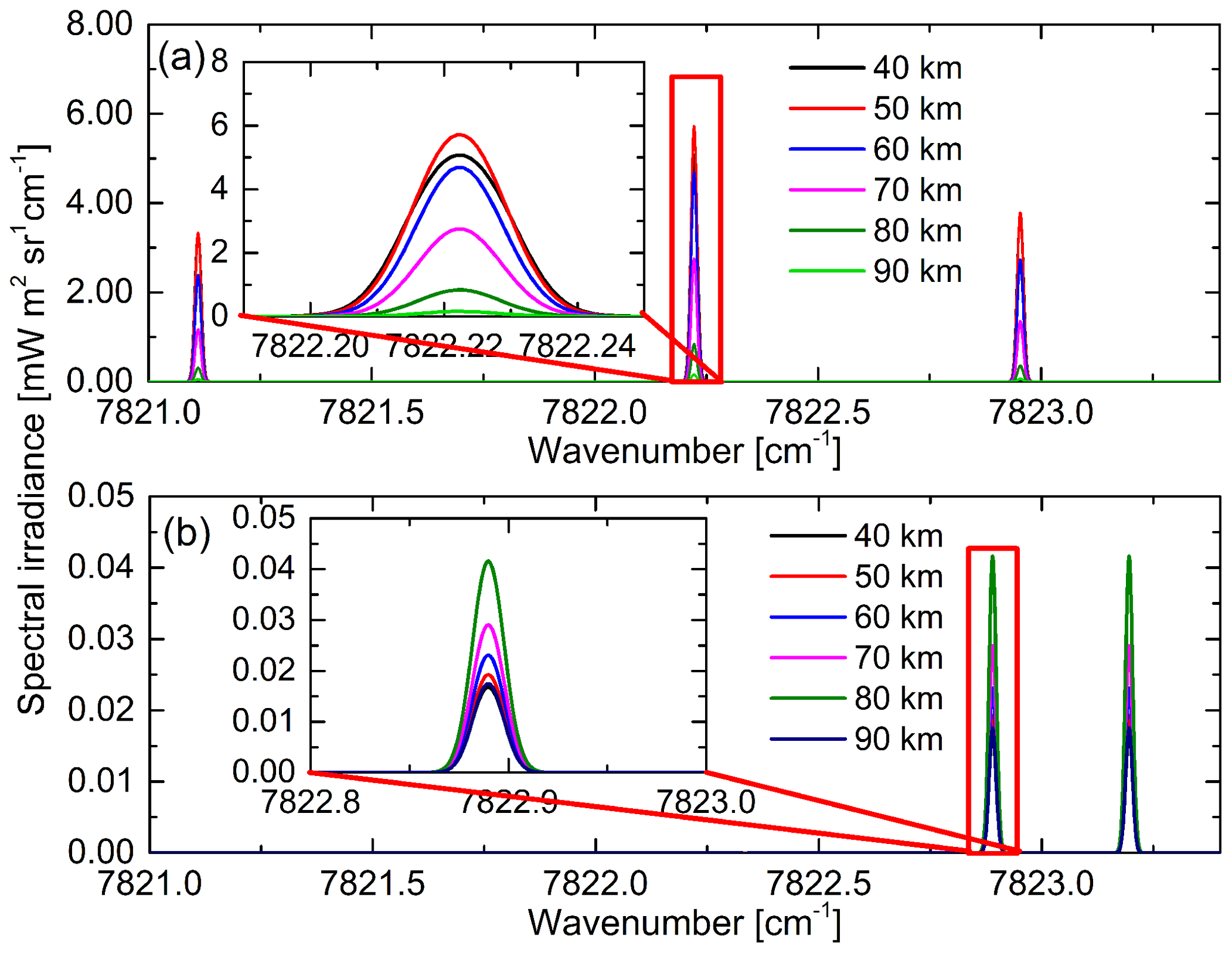
Figure 2The spectral irradiance of the three emission lines of O2 dayglow and the two emission lines of OH dayglow at tangent heights of 40, 50, 60, 70, 80 and 90 km. (a) Three emission lines of O2 dayglow. (b) Two emission lines of OH dayglow. The inset panels of (a) and (b) show a magnified view of a certain emission line of O2 and OH dayglow, from which the linewidth and intensity varying with tangent heights can be seen more clearly.
The total spectral irradiance including the weak group of the O2 dayglow and the OH dayglow is shown in Fig. 3a. The third emission line of the O2 dayglow near 7823 cm−1 is too close to the OH lines RR2.5e and RR2.5f (less than 0.05 nm) to be well isolated optically. Figure 3b shows the band radiance profiles of the O2(a1Δg) near 7823 cm−1 and the OH dayglow, and their ratio. As can be seen, the OH dayglow affects the observation of the O2 emission line near 7823 cm−1, especially for altitudes between 80 to 90 km where the OH dayglow is relatively strong.
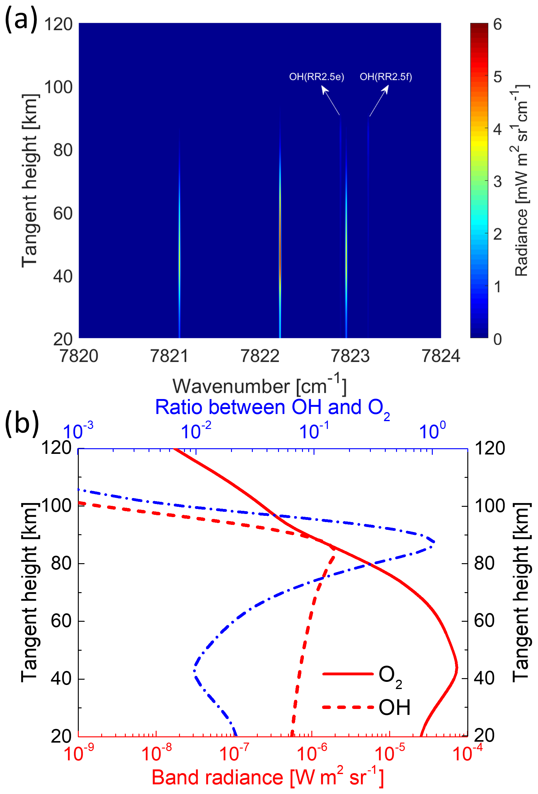
Figure 3The total spectral irradiance and band radiance as a function of tangent height. (a) The total spectral irradiance containing O2(a1Δg) and OH dayglow as a function of tangent height. (b) The band radiance profiles of the O2(a1Δg) and OH dayglow and their ratio.
The Doppler shift of the emission line due to the movement of the atmosphere is measured as a phase shift of the Michelson interferometer, and accurate temperature measurement is obtained from the integrated absorbance ratio of two isolated emission lines (He et al., 2019). However, the intensity variation caused by Doppler shift or temperature change is very small. The relative Doppler shift is w∕c, where w denotes the motion of the background atmosphere and c is the velocity of light. If winds are to be measured to an accuracy of 3 m s−1, a desirable value for the mesosphere and stratosphere, the measurement must be made to one part in 108 of the velocity of light. For the central wavelength of 1270 nm, that means the measurement of the wavelength shift is about 12 fm (femtometer). Since a linewidth of the O2 dayglow is of the order of 0.003 nm, the wavelength shift is of the linewidth. Therefore, the intensity variation of the band radiance near 7823 cm−1 caused by the existence of the OH dayglow will surely contribute to the increase in wind error, as well as the temperature error.
3.1 The instrument model
The NWTSI, using the combination of a “strong” emission lines group and a “weak” group of the O2(a1Δg) airglow, is a limb-viewing satellite instrument (He et al., 2019). The schematic drawing of the limb-imaging geometry and instrument concept is shown in Fig. 4, which closely follows the WAMI concept (Ward et al., 2001). The field of view (FOV) of NWTSI is defined by the first telescope with a value of , which allows NWTSI to cover an entire altitude range from 20 to 120 km in single images for a nominal spacecraft altitude of 410 km.

Figure 4Limb-imaging geometry and optical concept schematic drawing for NWTSI. The background map is from © NASA (https://eoimages.gsfc.nasa.gov/images/imagerecords/57000/57723/globe_west_2048.jpg, last access: 12 February 2020).
The entrance aperture of NWTSI is about 5 cm in diameter with an effective aperture ratio of f∕1.3. The magnifications of the first telescope and second are 2 and 0.5 respectively, so the FOV at the Michelson is and at the filters is again . The beam splitter of the NWTSI field-widened Michelson interferometer consists of two cemented half-hexagons with a low-polarizing semi-reflecting dielectric multilayer on one of the diagonal faces. It is made of BK7 glass and the entrance and exit faces are 6.35 cm2. Large optical path difference (OPD) and field widening involve using 12.240 cm LaKN12 glass and 11.070 cm BK7 glass with corresponding refractive indices 1.733 and 1.516 in the two arms of the interferometer. The OPD between the paths of the two arms of the Michelson interferometer for normal incident can be found from (He et al., 2019), which corresponds to a value of 7.35 cm. In order to avoid errors caused by intensity variations during measurements, the four interferogram samples are taken simultaneously rather than sequentially by dividing one Michelson mirror into four equal segments so the steps are coated permanently onto the mirror. A composite of etalon and interference filter is used to isolate individual emission lines. The etalon is fused silica with a finesse of 20 and a free spectral range of 2.0 nm. The etalon thickness is designed to give optimum transmittance in the outer one-third of the field of view for three strong and three weak O2 emission lines. The imaging system produces four copies of FOV by using a shallow, pyramid-shaped prism just in front of the camera. The edges of the prism are aligned with the divisions between the quadrants of the sectored Michelson mirror to form four images on the array detectors simultaneously, corresponding to different sampling steps of the Michelson segments.
3.2 The imaging interferogram
By sampling the interferogram for each pixel at four points corresponding to the four phase steps, the Doppler wind is obtained, which is so called the four-point sampling method. The equation representing the interferogram for a given pixel at row l and column j of the detector is (Rahnama et al., 2006)
where flj(ν) is the relative total filter function, Ulj is the instrument visibility, Δlj is the OPD, φklj is the Michelson interferometer kth phase step, and νis the wavenumber; the instrument responsivity Rlj is defined by
where AΩ is the pixel etendue, t is the exposure time, τ is the attenuation and q is the quantum efficiency.
The simulated mean value of the interferogram for the weak group of O2 dayglow as well as the OH dayglow is shown in Fig. 5. The pattern in Fig. 5a reflects the variation over the field of the filter transmittance function, the dependence of OPD on pixel positions and the tangent height variation of O2 dayglow within a column. The image in Fig. 5b shows the interference fringe of OH dayglow is much stronger for pixels nearer the periphery of the focal plane array (FPA), where the signal of the third weak emission line of the O2 dayglow near 7823 cm−1 is imaged.

Molecular species in NWTSI's selected spectral range of 7820–7824 and 7908–7912 cm−1 other than O2 can affect NWTSI's wind and temperature measurements through absorption and emission. Limb spectral radiance of OH airglow is the most important interfering constituent for NWTSI, especially for the weak group detection, as shown in Figs. 3 and 5. Using etalon as the ultra-narrow filter significantly reduces but does not eliminate the influence from OH airglow. Therefore, the uncertainty in its mixing ratio surely contributes to the increase in wind and temperature errors. Note that while the fabrication of this ultra-narrow filter with a spectral width of 0.1 nm is feasible for current technical levels and engineering capability, it would be extremely challenging to monitor the changes in its width and central wavelength during the mission.
The wind velocity vw is measured as a phase shift δφ of the interferogram
and phase φ can be calculated from
Fourier coefficients, J1, J2 and J3, also referred to as the apparent quantities, are related to any point k along a fringe interferogram I (Shepherd et al., 2012):
Omitting the presence of OH emission will change the value of J2 and J3, which will inevitably lead to an inversion error for the wind measurement.
The error standard deviation of inverted wind due to the presence of OH emission is found from the following relation (He et al., 2019):
where and represent the variance of the Fourier coefficients J2 and J3 due to the lack of knowledge on OH emission.
The contribution of OH dayglow to the wind error is shown in Fig. 6a. The black curve represents omitting the presence of the OH emission. As can be seen, the wind error is about 1–2 m s−1 for altitudes below 70 km, climbing to greater than 8 m s−1 as the altitude increases from 80 to 90 km. The sensitivity of wind retrieval is weaker in the lower altitudes due to the lower OH volume emission rate. The degree of knowledge of OH dayglow is important for NWTSI retrieval. The blue short-dash–dot line and the red short-dash line in Fig. 6a represent the error deviation of inverted wind with OH dayglow knowledge of 80 % and 90 %, respectively. As can be seen, when OH dayglow is known to 80 %, the wind error is 0.3–0.5 m s−1 for the altitude range of 40–70 km; for OH dayglow knowledge of 90 %, the wind error decreases to 0.1–0.3 m s−1.
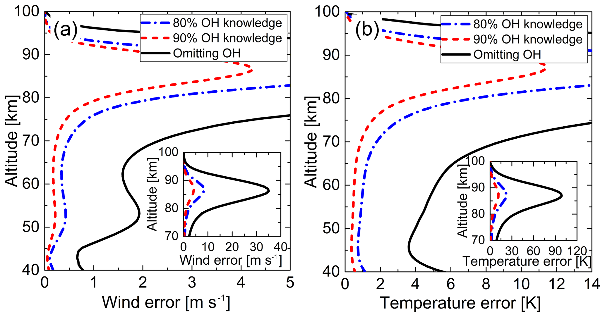
Figure 6Inversion errors in wind and temperature due to omitting the presence of OH dayglow (black curve) and with 80 % and 90 % knowledge of the OH dayglow (blue short-dash–dot line and the red short-dash line). (a) The wind error profiles. (b) The temperature error profiles. The inset panels of (a) and (b) show the wind and temperature error in the altitude range 70–100 km.
The error standard deviation of inverted temperature due to the presence of OH emission can be written as
where and represent the variance of the Fourier coefficients J1 of two emission lines A and B of the weak group of the O2 dayglow, and RAB is the ratio of the measured integral absorbances of this two lines, .
A similar trend with the wind error is found for the temperature obtained from J1A and J1B: the temperature error is about 4–6 K for altitudes below 70 km and greater than 20 K for altitudes from 80 to 90 km (see the black curve in Fig. 6b). When OH dayglow is known to 80 %, the temperature error is 0.7–1.0 K for the altitude range of 40–70 km (see the blue short-dash–dot line in Fig. 6b); for OH dayglow knowledge of 90 %, the temperature error decreases to 0.3–0.5 K (see the red short-dash line in Fig. 6b).
By happy coincidence, the wind and temperature inversion for altitude above 70 km is irrelevant to the weak group. Due to their relative weak self-absorption effect, the weak emission lines are used only for wind and temperature measurement at low altitude. The three strong emission lines suffering little from self-absorption at relatively higher tangent heights take the place of the weak group for data inversion.
The performance analyses presented assume that the OH dayglow is known to a degree that results in meeting the threshold wind and temperature accuracies. The largest errors are obtained when not accounting for OH dayglow in the retrievals. In order to bring down the wind and temperature error to an acceptable level, OH dayglow knowledge with an accuracy of 80 %–90 % is required.
We have simulated and discussed the effect of OH dayglow on the wind and temperature measurements derived from the 1.27 µm O2 dayglow limb-viewing observations. We first calculated the O2 and OH dayglow spectrum over the spectral region and altitude range of interest using the line-by-line radiative transfer model and the photochemical model incorporating the most recent spectroscopic parameters, rate constants and solar fluxes. They show that the OH lines RR2.5e and RR2.5f are too close to the third weak emission line of the O2 dayglow near 7823 cm−1 (less than 0.05 nm), which will surely affect the spectral integral intensity of the O2 mission line. A brief description of the instrument model of NWTSI including the schematic drawing of limb-imaging geometry and the instrument concept is presented. The method of four-point sampling of the interferogram and sample results of measurement simulations are provided for both O2 and OH dayglow. It was apparent from the simulations that the interference fringe of OH dayglow is much stronger for pixels nearer the periphery of FPA, where the signal of the third weak emission line of the O2 dayglow near 7823 cm−1 is imaged. Inversion errors of wind and temperature measurements due to the effect of OH dayglow are presented and discussed in detail. The presence of OH dayglow as an interfering species decreases the NWTSI performance at all altitudes, with the largest impact for altitudes from 80 to 90 km. The effect of OH dayglow on NWTSI inversion can be reduced by improving OH dayglow knowledge. Accurate OH(v=8) concentrations (uncertainty level of 20 % or better) are required to help meet the wind and temperature accuracy requirements.
Available upon request.
KW and WH conceived the ideas, developed the forward model, performed the measurement simulation and wrote the manuscript. YF helped in the instrument conceptualization and error analysis. YX calculated the atmospheric limb radiance. FL provided optical design expertise knowledge. All the authors contributed to the analysis and discussion of the results.
The authors declare that they have no conflict of interest.
The authors gratefully acknowledge informative and helpful discussions with Wang Dingyi on theoretical details of this work.
This research has been supported by the National Natural Science Foundation of China (NSFC) (grant nos. 41975039 and 61705253) and the National Key R&D Program of China (grant no. 2017YFC0211900).
This paper was edited by Ad Stoffelen and reviewed by two anonymous referees.
He, W., Wu, K., Feng, Y., Fu, D., Chen, Z., and Li, F.: The Near-Space Wind and Temperature Sensing Interferometer: Forward Model and Measurement Simulation, Remote Sens.-Basel, 11, 914, https://doi.org/10.3390/rs11080914, 2019.
Killeen, T. L., Wu, Q., Solomon, S. C., Ortland, D. A., Skinner, W. R., Niciejewski, R. J., and Gell, D. A.: TIMED Doppler Interferometer: Overview and recent results, J. Geophys. Res., 111, A10S01, https://doi.org/10.1029/2005JA011484, 2006.
Maihara, T., Iwamuro, F., Yamashita, T., Hall, D. N. B., Cowie, L. L., Tokunaga, A. T., and Pickles, A.: Observations of the OH airglow emission, Publ. Astron. Soc. Pac., 105, 940–944, https://doi.org/10.1086/133259, 1993.
Mlynczak, M. G., Solomon, S., and Zaras, D. S.: An updated model for O2(a1Δg) concentrations in the mesosphere and lower thermosphere and implications for remote-sensing of Ozone at 1.27 µm, J. Geophys. Res., 98, 18639–18648, https://doi.org/10.1029/93JD01478, 1993.
Mlynczak, M. G., Marshall, B. T., Martin-Torres, F. J., Russell, J. M., Thompson, R. E., Remsberg, E. E., and Gordley, L. L.: Sounding of the Atmosphere using Broadband Emission Radiometry observations of daytime mesospheric O2(a1Δg) 1.27 µm emission and derivation of ozone, atomic oxygen, and solar and chemical energy deposition rates, J. Geophys. Res., 112, D15306, https://doi.org/10.1029/2006JD008355, 2007.
Ortland, D. A., Skinner, W. R., Hays, P. B., Burrage, M. D., Lieberman, R. S., Marshall, A. R., and Gell, D. A.: Measurements of stratospheric winds by the high resolution Doppler imager, J. Geophys. Res., 101, 10351–10363, https://doi.org/10.1029/95jd02142, 1996.
Rahnama, P., Rochon, Y. J., Mcdade, I. C., Shepherd, G. G., Gault, W. A., and Scott, A.: Satellite Measurement of Stratospheric Winds and Ozone Using Doppler Michelson Interferometry. Part I: Instrument Model and Measurement Simulation, J. Atmos. Ocean. Tech., 23, 753–769, https://doi.org/10.1175/JTECH1880.1, 2006.
Russell, J. P. and Lowe, R. P.: Atomic oxygen profiles (80–94 km) derived from Wind Imaging Interferometer/Upper Atmospheric Research Satellite measurements of the hydroxyl airglow: 1. Validation of technique, J. Geophys. Res., 108, 4662, https://doi.org/10.1029/2003JD003454, 2003.
Shepherd, G. G., Thuillier, G., Cho, Y. M., Duboin, M. L., Evans, W. F. J., Gault, W. A., Hersom, C., Kendall, D. J. W., Lathuillere, C., Lowe, R. P., McDade, I. C., Rochon, Y. J., Shepherd, M. G., Solheim, B. H., Wang, D. Y., and Ward, W. E.: The Wind Imaging Interferometer (WINDII) on the Upper Atmosphere Research Satellite: A 20 Year Perspective, Rev. Geophys., 50, 713–723, https://doi.org/10.1029/2012RG000390, 2012.
Song, R., Kaufmann, M., Ungermann, J., Ern, M., Liu, G., and Riese, M.: Tomographic reconstruction of atmospheric gravity wave parameters from airglow observations, Atmos. Meas. Tech., 10, 4601–4612, https://doi.org/10.5194/amt-10-4601-2017, 2017.
Ward, W. E., Gault, W. A., Shepherd, G. G., and Rowlands, N.: The Waves Michelson Interferometer: A visible/near-IR interferometer for observing middle atmosphere dynamics and constituents, Proc. SPIE, 4540, 100–111, https://doi.org/10.1117/12.450652, 2001.
Ward, W. E., Gault, W. A., Rowlands, N., Wang, S., Shepherd, G. G., McDade, I. C., McConnell, J. C., Michelangeli, D., and Caldwell, J.: An imaging interferometer for satellite observations of wind and temperature on Mars, the Dynamics Atmosphere Mars Observer (DYNAMO), Proc. SPIE, 4833, 226–236, https://doi.org/10.1117/12.473823, 2002.
Wu, K. J., Fu, D., Feng, Y. T., Li, J., Hao, X. B., and Li, F. Q.: Simulation and application of the emission line O19P18 of O2(a1Δg) dayglow near 1.27 µm for wind observations from limb-viewing satellites, Opt. Express, 26, 16984–16999, https://doi.org/10.1364/OE.26.016984, 2018.
Zhang, R., Ward, W. E., and Zhang, C. M.: O2 nightglow snapshots of the 1.27 µm emission at low latitudes on Mars with a static field-widened Michelson interferometer, J. Quant. Spectrosc. Ra., 203, 565–571, https://doi.org/10.1016/j.jqsrt.2017.08.009, 2017.