the Creative Commons Attribution 4.0 License.
the Creative Commons Attribution 4.0 License.
 | 15 May 2020
Single-photon laser-induced fluorescence detection of nitric oxide at sub-parts-per-trillion mixing ratios
Andrew W. Rollins
Pamela S. Rickly
Ru-Shan Gao
Thomas B. Ryerson
Steven S. Brown
Jeff Peischl
Ilann Bourgeois
We describe a newly developed single-photon laser-induced fluorescence sensor for measurements of nitric oxide (NO) in the atmosphere. Rapid tuning of a narrow-band laser on and off of a rotationally resolved NO spectral feature near 215 nm and detection of the red-shifted fluorescence provides for interference-free direct measurements of NO with a detection limit of 1 part per trillion by volume (pptv) for 1 s of integration, or 0.3 pptv for 10 s of integration. Uncertainty in the sensitivity of the instrument is typically ±6–9 %, with no known interferences. Uncertainty in the zero of the detector is shown to be <0.2 pptv. The instrument was deployed on the NASA DC-8 aircraft during the NASA/NOAA FIREX-AQ experiment (Fire Influence on Regional to Global Environments Experiment – Air Quality) during July–September 2019 and provided more than 140 h of NO measurements over 22 flights, demonstrating the ability of this instrument to operate routinely and autonomously. Comparisons with a seasoned chemiluminescence sensor during FIREX-AQ in a variety of chemical environments provides validation and confidence in the accuracy of this technique.
- Article
(3908 KB) - Full-text XML
- BibTeX
- EndNote


Nitric oxide (NO) is central to radical chemistry in Earth's atmosphere. In the troposphere the catalytic reaction of NO with the hydroperoxy and organic peroxy radicals
is frequently the rate-limiting step for the production of tropospheric ozone (O3) and is the reason why anthropogenic emissions of NO result in a buildup of O3 pollution (Laughner and Cohen, 2019). Oxidation of NO ultimately also results in the formation of nitric acid and consequently nitrate aerosols and nitrogen deposition. NO has an important control over the partitioning of atmospheric HOx () due to the reaction between NO and the hydroperoxyl radical (Gao et al., 2014). Stratospheric NOx () is important for suppressing concentrations of chlorine monoxide (ClO) which leads to rapid destruction of O3 (Fahey et al., 1993; Solomon, 1999). Increases in stratospheric aerosols lead to more rapid heterogeneous conversion of NOx into nitric acid and consequently an increase in ClO: a potential by-product of future solar radiation management efforts (Tilmes et al., 2018).
Active fields of atmospheric research seek to understand radical chemistry cycling in low-NO regimes. Hydroxyl radical budgets in forested environments where NO measurements are near 10 parts per trillion by volume (pptv, 10−12 mol mol−1) remain incompletely understood, with measurements of OH frequently exceeding calculated OH. While many of the model–measurement discrepancies reported in the past have now been attributed to artifacts in the HOx measurements, new low-NO chemistry continues to be discovered that helps to bridge this gap (Fittschen et al., 2019). Autoxidation of organic compounds in low-NO environments is increasingly recognized as a key source of highly oxidized/low-volatility organic compounds in the atmosphere (Crounse et al., 2013). Measurements of the ratio of NO to nitrogen dioxide (NO2) in the upper troposphere (UT) frequently cannot be reconciled with models (Cohen et al., 2000; Silvern et al., 2018). Zhao et al. (2019) show that differences in background NO at the single pptv level are responsible for differences in global modeled OH on the order of 50 %. The ability to measure atmospheric NO at very low mixing ratios and with low uncertainty will be crucial to address these and other questions in atmospheric chemistry research for the foreseeable future.
Almost all of the research in the past 2 decades associated with direct detection of atmospheric NO has relied on the chemiluminescence (CL) detection technique (Ridley and Howlett, 1974). In this method, a sample of air is mixed with a high concentration (∼1 %) of O3, resulting in the formation of electronically excited nitrogen dioxide, which produces intense luminescence in the near infrared. This technique, while being quite precise (∼5–10 pptv detection limit), has significant drawbacks. These include potential positive or negative interferences from other species, including a variety of organic compounds (Drummond et al., 1985); precision limits on the order of 5–10 pptv; significant instrumental background levels (10–100 pptv equivalent), which might reduce accuracy; reliance on consumables, including pure oxygen and cryogen (required for cooling detectors in high sensitivity CL instruments); and production of percentage levels of ozone, which is toxic and must be exhausted from the instrument.
An alternative direct technique which has been explored previously is laser-induced fluorescence (LIF). Due to the NO absorption cross sections in the deep ultraviolet region of greater than 10−16 cm2 molecule−1 and moderately high fluorescence quantum yield (∼10 %), it should be expected that very precise NO measurements could be made using such a technique. Atmospheric measurements using both single-photon and two-photon excitation schemes were demonstrated by Bradshaw et al. (1982, 1985) and Bloss et al. (2003). The single-photon excitation scheme employed by Bradshaw et al. used a dye-based laser system near 226 nm to excite the manifold of the A2Σ electronic state and observe the red-shifted fluorescence emission from relaxation near 259 nm (). This system had a reported detection limit of 28 pptv for 1 min of integration. The two-photon scheme (Bradshaw et al., 1985) involved further excitation of NO that had been pumped into the A2Σ state using a second photon at 1.06 µm to promote NO into the D2Σ state. The highly excited NO would emit blue-shifted fluorescence at 187 nm, which had the advantage of being detected on a near-zero background. The reported detection limits for this technique were 1 pptv given 5 min of integration, or 10 pptv for 30 s of integration (Bradshaw et al., 1985). To our knowledge, the two-photon scheme developed by Bradshaw et al. is the only NO-LIF measurement that has been utilized extensively for atmospheric measurements including on aircraft, and this technique was last successfully used during the NASA TRACE-P experiment in 2001. Field comparisons of the two-photon excitation scheme with multiple CL instruments demonstrated similar performance for the two techniques (Hoell et al., 1987). Bloss et al. (2003) used a frequency quadrupled Ti:sapphire laser system to excite NO near 226 nm and detected broadband red-shifted fluorescence at 240–390 nm. Although Bloss et al. did not state a detection limit for their prototype instrument, they calculated that a detection limit of 0.07 pptv for 60 s of signal integration might be achievable with improvements in their system. More recently Mitscherling et al. (2007, 2009) reported investigation of the use of single-photon LIF detection of NO for human breath analysis by pumping the A2Σ←X2Π transition both near 226 nm () and near 215 nm ().
In this work we report on the recent development of a new single-photon LIF sensor that pumps the vibronic transition near 215 nm and observes the resulting red-shifted fluorescence from ∼255 to 267 nm. The present system is distinguished from previous efforts to use LIF to measure atmospheric NO primarily because we use a fiber-amplified laser system. This system has numerous advantages, including (1) laser linewidth that is sufficiently narrow to resolve the Doppler broadened NO spectrum at room temperature and thereby achieve high signal levels and distinguish the NO isotopologues; (2) laser repetition rate high enough to enable single-photon counting of the fluorescence signal; and (3) size, weight, and environmental robustness allowing for practical and routine integration onto airborne research platforms. The current version of this system has a detection limit (2σ) of ∼1 pptv for 1 s of integration, or ∼0.3 pptv for 10 s of integration. Uncertainty in the instrument zero is demonstrated to be less than 0.2 pptv. The instrument was integrated onto the NASA DC-8 aircraft during the NASA/NOAA FIREX-AQ experiment (Fire Influence on Regional to Global Environments Experiment – Air Quality) during 2019. Here we describe the instrument and its performance during this initial deployment.
2.1 Instrument description
In this section we describe the physical components of the LIF instrument. Subsequent sections discuss details of the NO spectroscopy and instrument performance.
The laser and optical detection system used here are based on that originally described by Rollins et al. (2016) for measurements of sulfur dioxide. Subsequent to that work, important changes have been made to the design of the fiber laser system, and therefore a complete description is provided here.
The laser wavelength is controlled by modulating the current of a distributed feedback (DFB) laser. This fiber-coupled DFB laser can provide up to 50 mW continuous optical power in a single-mode polarization-maintaining fiber and can be tuned in the range of 1074–1076 nm with a nominal linewidth of 10 MHz. The DFB output is chopped to make pulses of 2–3 ns in duration with a 320 kHz repetition rate using a fiber-coupled electro-optic modulator with 10 GHz of switching bandwidth and an extinction ratio of 40 dB. The ∼40 pJ pulses are amplified in a multi-stage ytterbium-doped fiber amplifier to near 5 µJ and then exit the fiber-amplifier system through an end-capped fiber, and the beam is collimated to a diameter of 350 µm.
The pulses pass through three nonlinear crystals to produce the fifth harmonic near 215 nm with a yield of ∼1 %. The first crystal is a type-II phase-matched KTP crystal ( mm) producing the second harmonic at 537.5 nm. The second crystal is a type-I phase-matched LBO crystal ( mm) which mixes the 537.5 nm light with the residual 1075 nm light to produce the third harmonic at 358.3 nm. A dual-wavelength wave plate (λ∕2 @ 537.5 nm, λ @ 358.3 nm) rotates the residual second harmonic beam to be parallel with the third harmonic beam. A 40 mm focal length lens is then used to slightly focus the beams into a type-I phase-matched BBO crystal ( mm) producing the fifth harmonic near 215 nm. A Pellin–Broca prism separates the harmonics, and all of the light is trapped except for the 215 nm beam, which is steered into the LIF cell.
Figure 1 depicts the layout of the free-space portion of the optical system and the NO detection system. The 215 nm beam, which is typically near 1 mW, passes through the fluorescence sample cell a single time. The beam is then split about 10∕90, with 10 % of the power entering a solar-blind power-monitoring phototube (Hamamatsu R6800U-01) and 90 % passing through a reference fluorescence cell and into a second phototube. The reference cell typically has a constant flow of 500 ppbv NO flowing at 50 standard cubic centimeters per minute (sccm), and the exhaust of the cell is tied to the exhaust of the sample cell such that both cells are at pressures within 0.5 hPa during measurements. The absolute pressure that is maintained in the cells depends on the experiment and the maximum altitude that the aircraft will reach but is typically in the range of 40–100 hPa (see Sect. 2.4). Inside each cell, a quartz lens with numerical aperture of 0.5 collects fluorescence light from the center of the cell, which then passes through a 260±8 nm bandpass filter (Semrock FF01-260/16) and is then imaged onto the photocathode of a photomultiplier tube (PMT) module operated in single-photon-counting mode (Hamamatsu H12386-113). The fluorescence axis with the collection optics, bandpass filters, and PMTs is perpendicular to both the flow and laser axes. For clarity, these components are omitted from Fig. 1. In the reference cell, it is necessary to reduce the signal on the PMT to maintain a response that is linear with changes in laser power. Therefore a neutral density filter with a typical optical depth (OD) of 1.0 is placed between the bandpass filter and the PMT. The combination of 500 ppb NO and the OD =1.0 filter maintains a high signal : noise ratio in the reference cell while allowing for the same bottle of NO to be used both to supply the reference cell and to calibrate the instrument sensitivity (typically a 5 ppmv standard that is diluted for the reference cell).

Figure 1Schematic of the free-space optical layout. The fluorescence collection optics, bandpass filters, and PMTs for both the measurement and reference cells are located above this plane and are omitted for clarity. These components are located above the center of each cell and image light from the center of the cells onto the PMTs. In the measurement cell, most of the sample air passes straight through the cell to quickly flush the volume in the middle of the cell that is imaged onto the PMT. A minor fraction of the sample air is drawn out through the arms of the LIF cell to reduce dead volumes in the measurement volume.
The sample flow and pressure are controlled by two custom stepper-motor-controlled butterfly valves that are designed to minimize pressure drop through the system and potential sampling artifacts (Gao et al., 1999). The inlet valve is machined out of PEEK material (polyether ether ketone), and the exhaust valve out of stainless steel. PEEK has been found to be quite machinable while maintaining chemical inertness and shows no signs of producing a sampling artifact. The inlet valve is continuously adjusted to maintain constant flow (typically 2500 sccm) using feedback from a mass flow meter that measures the exhaust of the sample cell. While most of the sample flow passes directly through the cell and is exhausted opposite the inlet, a small fraction of the sample flow is exhausted through the arms of the cell to minimize dead volumes within the cell. The exhaust valve, which is located after the point where the sample and reference cell exhausts are tied together, is adjusted to maintain a constant pressure measured immediately downstream of the sample cell. During flight operation on the DC-8, the pressure and flow were always maintained to within a 1 % range of their set points over the entire altitude range encountered including during ascent and descent legs. Flow through the reference cell is controlled using a pair of mass flow controllers to mix zero air (NO<2 pptv) and gas from a NO standard gas cylinder.
Data collection and instrument control are performed using a National Instruments CRIO data system. This system incorporates a field-programmable gate array which is used to control the timing of the laser and photon detection gating with a precision of 5 ns. The instrument that was designed for operation on the NASA DC-8 aircraft houses the detection and reference cells, gas deck, and data system in one enclosure ( cm) and the fiber laser components in a second enclosure ( cm). In total, these occupy 26 cm of vertical rack space in a standard instrumentation rack and weigh 31 kg. Typically, a vacuum scroll pump (Agilent IDP-3) and a small calibration gas bottle are installed in the rack adjacent to the instrument. These components take another 21 cm of vertical rack space and weigh 19 kg.
2.2 NO spectroscopy
Figure 2 illustrates the relevant NO electronic potential energy surfaces and the LIF scheme used in this work. We pump the transition near 215 nm, and observe the resulting red-shifted fluorescence from the transitions.

Figure 2Energy level schematic of NO-LIF system. Schematic is qualitative and not intended to be to scale.
The rovibronic spectrum of NO, especially in the “gamma bands” (A2Σ←X2Π), has been the subject of numerous previous studies (see Mitscherling, 2009, and references therein). Figure 3 illustrates the absorption spectrum of NO. Line-by-line-resolved spectra shown here have been calculated using the PGOPHER software package (Western, 2017). For the simulation of 14N16O absorption spectra we use the spectroscopic data reported by Danielak et al. (1997) and Murphy et al. (1993).
The tunable laser used here pumps NO near 215 nm from the ground state into the state. Using this excitation has multiple advantages over the excitation scheme pumping at 226 nm used by Bradshaw et al. (1982). First, the absorption cross section (σ) for NO is about twice as high in the 1←0 transition compared to 0←0. Second, the additional vibrational energy provides a more significant shift in the spectra of the various NO isotopologues, making them more easily distinguished spectroscopically. The origin of the transition for 14N16O is 46 and 70 cm−1 higher in energy than those for the 15N16O and 14N18O isotopologues. Third, 215 nm can be produced using the fifth harmonic of a ytterbium-doped fiber-amplifier system operating at 1075 nm, whereas 226 nm cannot currently be produced using such a system. In addition, excitation at 226 nm has the potential to produce spurious signal from fluorescence of SO2, while 215 nm is a minimum in the SO2 absorption cross section, and the SO2 fluorescence quantum yield here is less than 3 % (Hui and Rice, 1973).
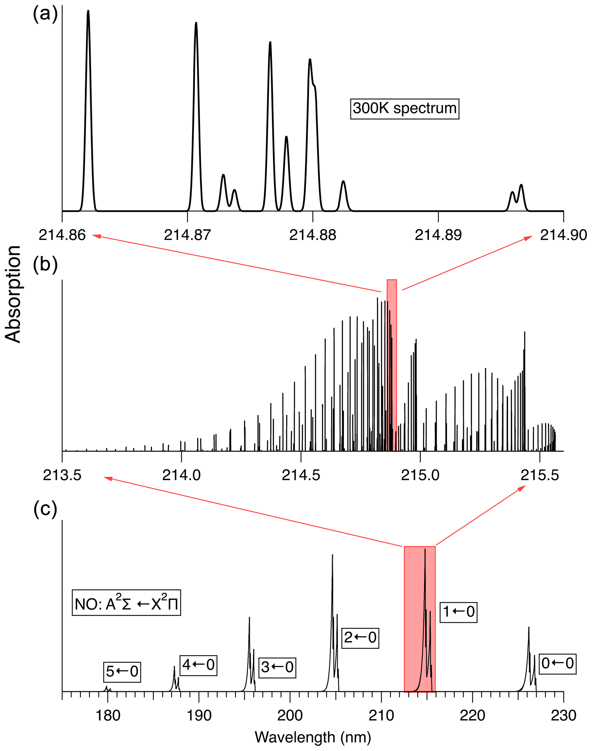
Figure 3Spectrum of the A2Σ←X2Π transition in NO at 300 K. (c) shows the absorption spectrum in low resolution. (b) shows the calculated stick spectrum for the 1←0 transition. (a) shows the spectral region used here to measure NO, convolved with a 0.1 cm−1 width Gaussian lineshape, which is the Doppler linewidth of NO at 300 K.
Figure 4 shows the expected fluorescence emission spectrum based on the Franck–Condon factors (Scheingraber and Vidal, 1985; Danielak et al., 1997). Excluding the emission at , which cannot be distinguished from Rayleigh scatter, fluorescence from the state is expected to peak at (255 nm) or (267 nm) although it should be possible to collect significant signal within the range of –8 (Scheingraber and Vidal, 1985). Multiple detection bandpass filters were tested to optimize the signal : noise ratio for NO detection. The signals obtained with filters collecting the 1→4, 1→5, and 1→6 transitions scaled relative to each other as expected with the Franck–Condon factors for those transitions. Of the filters tested, the one found to produce the lowest detection limit is a filter centered at 260 nm with a full width of 16 nm (see Fig. 4). This has 63 % transmission at the 1→4 transition (255 nm) and 69 % transmission at 1→5 (267 nm) while completely rejecting laser Rayleigh and Raman scatter from N2 and O2. While operating the detection cell near 80 hPa, typical background using this filter is 10 counts s−1 with 1 mW laser power. Of this background, about 1 count s−1 is a dark count from the detector. Using a filter to additionally collect the 1→6 emission not only increased the signal by 4.5 counts s−1 mW−1 pptv−1 but also increased the background to more than 350 counts s−1 mW−1, which would significantly degrade the detection limit. We expect that background levels would only further increase at longer collection wavelengths while collecting the fluorescence from at 244 nm would likely increase the signal without substantial increases in the background.
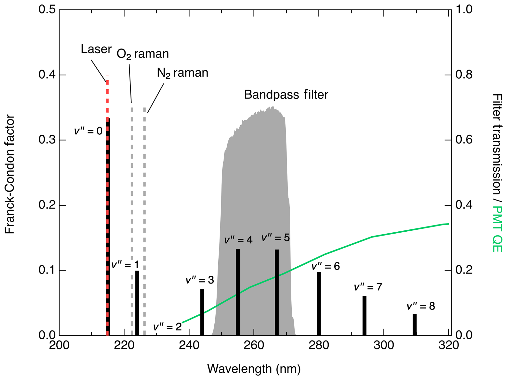
Figure 4Franck–Condon factors (black sticks plotted on left axis) indicating the expected distribution of the fluorescence intensity from the relaxation. Grey shaded region (right axis) shows detected spectral region in this work. Locations of significant scatter from Rayleigh, O2 Raman, and N2 Raman are also indicated. Green line plotted against the right axis shows the quantum efficiency (QE) of the PMT module used in this work.
2.3 LIF signal
The anticipated LIF signal (S, counts s−1) is proportional to the product of the NO excitation rate E(ν) (s−1), the fluorescence quantum yield ϕ, and the fluorescence collection efficiency of the detection system Ω.
In the optically thin regime, E(ν) can be approximated as the product of the convolution of the molecular absorption cross section (σ(ν) (cm2 molecule−1)) with the normalized laser spectral distribution (Λ(ν)), the concentration of NO in the sample cell (n, molecule cm−3), the volume within the sample cell that is illuminated and imaged onto the PMT (V, cm3), and the laser photon flux in the sample volume (Φ, photons s−1 cm−2).
We excite NO near 214.8800 nm (46537.64 cm−1) at an envelope with four overlapping rotational lines (Q-branch and P-branch ). The peak of the absorption cross section in this envelope at 300K is cm2 molecule−1. Because the laser used here has a linewidth that is comparable to the Doppler broadened linewidth of NO at 300 K (ΔνDoppler=3 GHz), we approximate the convolution of the NO cross section with the laser lineshape as cm2 molecule−1. In reality, the non-negligible laser lineshape in the current system slightly reduces the effective σ. In comparison, Bradshaw et al. (1982) reported an effective cross section of cm2 molecule−1 due to their wider laser spectrum. A typical cell pressure that has been used in the laboratory and can be maintained during aircraft sampling up into the lower stratosphere is 42.5 hPa (1.05×10¹⁸ molecules cm−3). Therefore, at a NO mixing ratio of 1 pptv the NO concentration in the cell would be molecules cm−3. We estimate that a cubic volume with an edge of about 5 mm is imaged onto the PMT. With a typical laser power of 1 mW at 215 nm the photon flux is photons s−1 cm−2. Therefore the estimated excitation rate is 86 625 s−1 pptv−1 mW−1.
The fluorescence quantum yield ϕ is determined by the competition between the natural fluorescence lifetime of NO* and collisional quenching by other molecules in the sample gas. The natural radiative lifetime of is 200 ns ( s−1) (Luque and Crosley, 2000). The primary quenchers in the atmosphere are expected to be N2, O2, and Ar. Nee et al. (2004) measured the quenching rate coefficients for NO by N2, O2, and Ar to be , , and cm3 molecules−1 s−1, respectively. Therefore in dry air with 78 % N2, 21 % O2, and 1 % Ar, the quenching rate is s−1. Carbon dioxide is also a fast quencher of NO*, () (Nee et al., 2004), and 400 ppm of CO2 would increase the fluorescence quenching rate by 0.4 %. For measurements of NO near very large CO2 sources this additional quenching might need to be considered. Water vapor also has an important and variable effect on ϕ, and this is addressed in a subsequent section. In 42.5 hPa of dry air, we therefore expect the fluorescence quantum yield to be
Similarly, the e-folding lifetime of the fluorescence signal in these conditions is calculated to be 26 ns. By adjusting the photon-counting gates in our system in 5 ns increments, we determined the signal lifetime at a range of pressures from 14.7 to 103.5 hPa. A Stern–Volmer analysis of the observed lifetimes concluded that the natural radiative lifetime τr is 180 ns, and the quenching rate in dry zero air (no CO2) is cm3 molecules−1 s−1, overall in good agreement with the literature values of 200 ns and cm3 molecules−1 s−1. Because the lifetime of the signal at typical cell pressures is short (i.e. 26 ns) and the optical background is already quite low, we have not observed in improvement in signal : noise ratio by temporally gating out the prompt scatter. Therefore, during NO measurements we typically use a photon collection gate near 50 ns that overlaps the laser pulse and collects >80 % of the potential signal. Use of this gate primarily reduces the effect of PMT dark counts from the nominal rate of 50 s−1 to <1 s−1.
The fluorescence collection efficiency is determined by the product of the optical bandpass filter transmission with the geometric collection efficiency and the quantum efficiency of the PMT. The Franck–Condon factor for the transition is 0.13 (Danielak et al., 1997) and the bandpass filter transmission at 255 nm is 0.63, while the Franck–Condon factor for is also 0.13 (Danielak et al., 1997) and the bandpass filter transmission at 267 nm is 0.69. The 0.5 NA lens captures 0.067 of the fluorescence emitted from the center of the cell. At best, a mirror opposite the lens increases this collection by a factor of 1.5, bringing the geometric collection efficiency to 0.1. The quantum efficiency of the PMT at 255–267 nm is ∼0.2. Thus, the fluorescence collection efficiency of the system is .
Taking the product of the excitation rate with the fluorescence quantum yield and fluorescence collection efficiency, we estimate that the anticipated signal rate is approximately 38 counts s−1 pptv−1 mW−1. The anticipated signal level is comparable to the fluorescence sensitivity that has been measured for this instrument (11.3 counts s−1 pptv−1 mW−1; see Fig. 10). The comparison between the theoretical sensitivity and measured sensitivity is quite reasonable given uncertainties in a number of the parameters discussed above.
2.4 Temperature, pressure, and water vapor dependence
The absorption cross section is proportional to the rotational populations in the ground states that are being probed (), and, therefore, a temperature dependence to the signal is anticipated. Near 300 K, populations in all of the probed rotational states will decrease with increasing temperatures. Figure 5 shows the calculated temperature dependence of the Doppler broadened absorption cross section relative to 300 K at 214.880 nm. In this region, a relative decrease in sensitivity of 0.34 % K−1 is calculated.
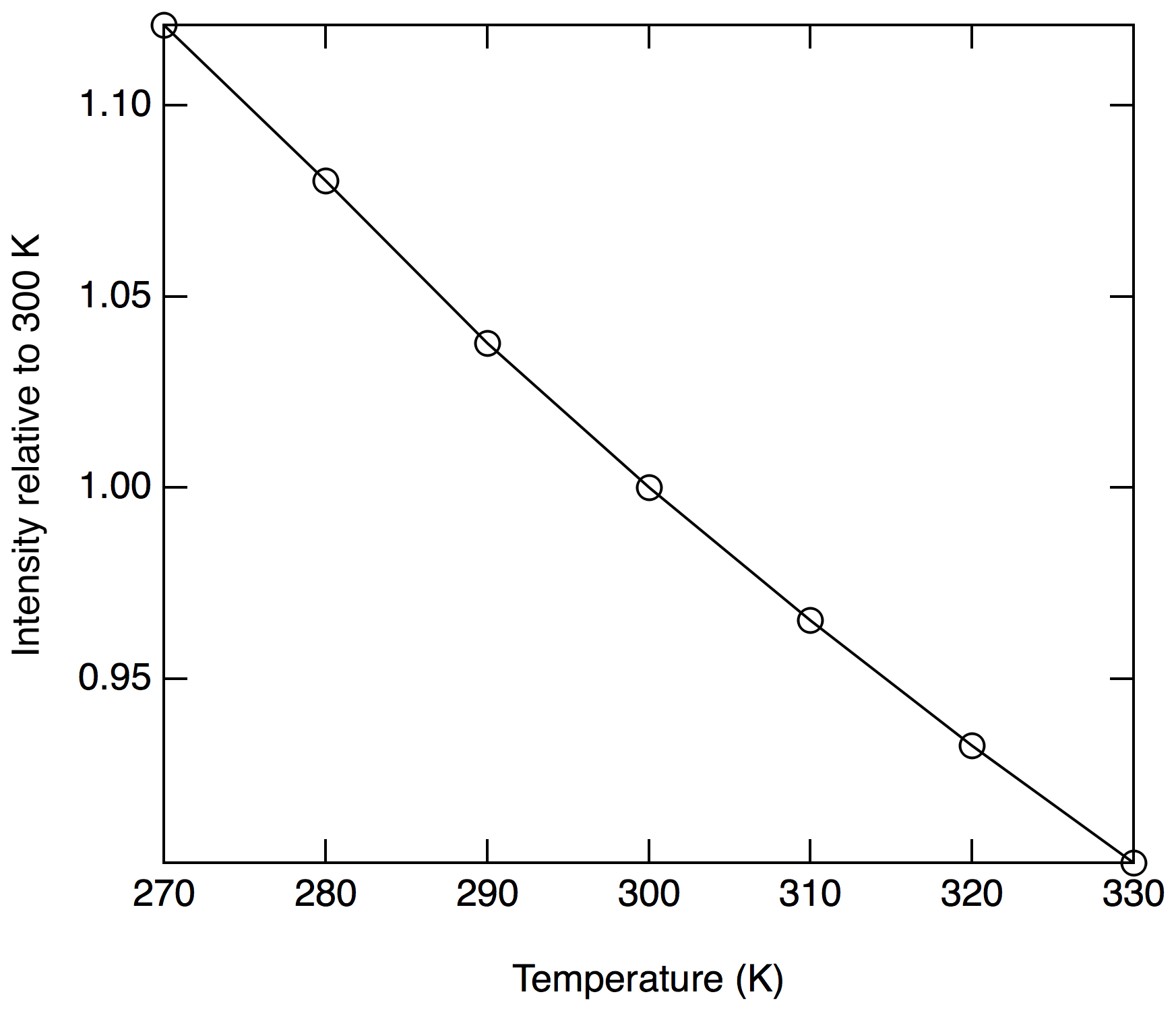
If changes in the sample temperature were identical to changes in the temperature of the gas in the reference cell, any sensitivity changes would be exactly accounted for during data reduction. If significant differences arose in the gas temperatures between the sample and reference cells, an artifact would arise. For ground-based measurements, the temperatures of the sample cell, reference cell, and sample gas flow will usually be very similar. For aircraft measurements where gas from the cold atmosphere (as low as −90 ∘C) is rapidly drawn into a warmer analysis region, care must be taken to ensure the probed sample gas is well thermalized with the measurement cell and that the reference cell is close in temperature.
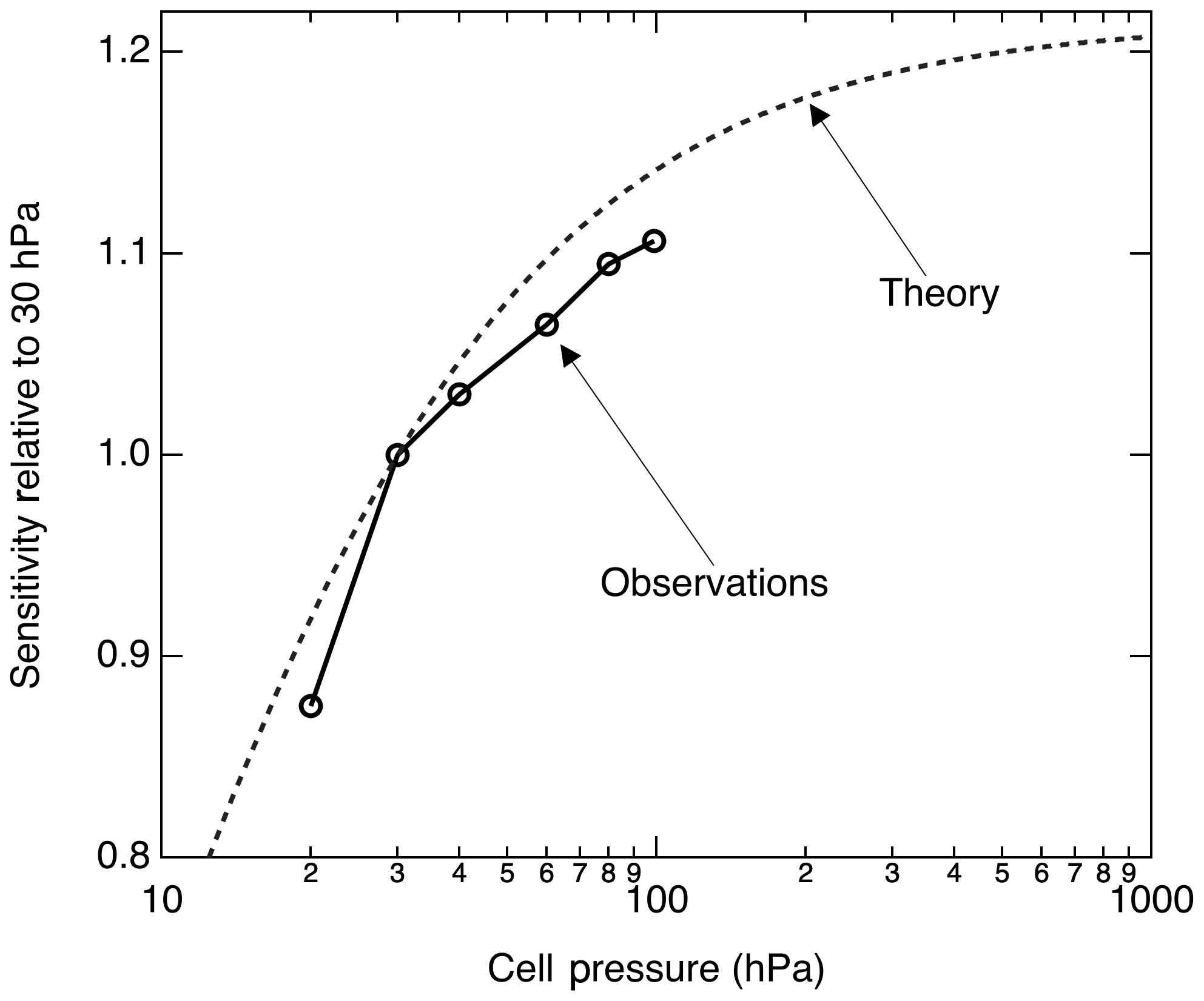
The pressure dependence of the signal arises due to changes in both the excitation rate E(ν) and the fluorescence quantum yield ϕ. The excitation rate is directly proportional to the NO concentration in the cell and will increase linearly with pressure at a constant NO mixing ratio. In the low pressure limit, ϕ is independent of pressure; in the high pressure limit, ϕ is inversely proportional to the pressure. Thus, at low pressures the LIF signal increases with pressure and eventually the signal becomes independent of pressure.
Figure 6 shows the calculated pressure dependence of the LIF sensitivity based on the previously cited fluorescence and quenching rates. We measured the LIF sensitivity between 20 and 100 hPa and show that it generally follows the anticipated pressure dependence. At 100 hPa, we observed ≈ 10 % more sensitivity than we do at 30 hPa. Significantly higher pressures reduce the instrumental response time and cannot be maintained on aircraft in the upper troposphere with sufficient flow.
Quenching of NO* due to water vapor is fast and must be considered in humid environments. While a quenching rate coefficient () of the state has not been reported, Paul et al. (1996) reported for quenching of the state cm3 molecules−1 s−1. Based on the very small differences between quenching rates for the and states by N2 and O2 (Nee et al., 2004), it was expected that quenching by H2O of is reasonably close to the value measured for and therefore would be important for high humidities.
Quenching by H2O will decrease the sensitivity of the instrument to NO by introducing an additional term in the fluorescence quantum efficiency:
When ϕ0 is defined as the fluorescence quantum efficiency at zero H2O concentration, it follows that
Therefore, a plot of the inverse of the relative LIF signal (S0∕S) as a function of [H2O] will yield a line with a slope equal to . For cell pressures of 42.5 and 85.4 hPa we measured S0∕S for a range of H2O mixing ratios and used this analysis to determine . For these experiments, mixtures of 5 ppb NO in zero air under a range of humidities were generated using varying mixtures of saturated zero air and dry zero air. The mixture was sampled in parallel by the LIF instrument and an MBW 373LX chilled-mirror hygrometer (MBW Calibration AG). Using this analysis and assuming s−1 and cm3 molecules−1 s−1, the data from 42.5 and from 85.4 hPa suggest that is and cm3 molecules−1 s−1, respectively. The discrepancy between these results could arise from small errors in any of the parameters – kr, kair, [M], or [H2O] – used to derive these values. In Fig. 7 we show the observed relative signals as a function of H2O at the two cell pressures. A mean value of of cm3 molecules−1 s−1 is used to reasonably reproduce the observations at both cell pressures.
Figure 7(a) Markers show the observed S∕S0 values, and dashed lines show the calculated S∕S0 values using cm3 molecules−1 s−1. (b) Relative difference between observed and calculated S∕S0 values shown in (a).
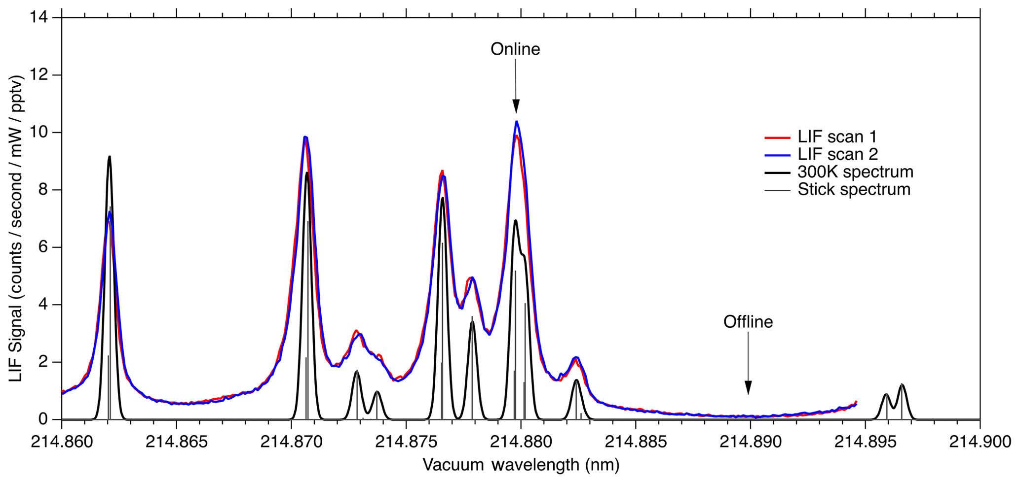
Figure 8LIF signal observed during laser scans compared to calculated absorption cross section at 300 K.
Figure 7 shows that the decrease in the LIF sensitivity to NO under humid conditions is quite substantial (e.g., a 29 % decrease in signal at 20 000 ppm H2O). However, this change in instrument sensitivity is well understood and can be characterized with high accuracy for a known or constant LIF cell pressure. Figure 7b shows that, at up to 20 000 ppm H2O, differences of up to 3 % are observed between the laboratory observations and the model. We note that, for such a H2O-dependent sensitivity to be applied during data reduction, good-quality measurements of H2O mixing ratios are required and the uncertainty in the H2O measurements will contribute to the uncertainty in the calculated NO mixing ratio.
To test for the ability of in situ H2O measurements to account for the reduced fluorescence quantum yield, we performed standard addition calibrations of NO into both ambient and dry zero air during DC-8 flights for the FIREX-AQ experiment. A typical calibration sequence involved a 30 s period of adding 5 sccm of 5 ppmv NO into the normal sample flow of 2500 sccm, followed by 30 s where the ambient flow was also displaced using dry zero air. For each pair of measurements, the ambient water vapor mixing ratio was determined using a Los Gatos Research analyzer for N2O, CO, and H2O (LGR). Data from those calibrations are shown in Fig. 7. The effect of H2O on the NO signal as determined both in laboratory and on the DC-8 agree quite well, with maximum differences near 2 %. At H2O mixing ratios greater than ∼15 000 ppmv, the differences between the model and in situ observations diverge somewhat, with maximum differences of 4 %.
Figure 8 shows the fluorescence signal that is typically observed when scanning the seed laser current in the region used for NO measurements. We show two equivalent laser scans on a sample of 10 ppbv NO calibration gas. Each scan shows about 15 s of data acquisition. The observed fluorescence spectrum is plotted on top of a theoretical absorption spectrum that has been calculated using the PGOPHER program at a temperature of 300 K. The wide wings of the observed spectral lines are believed to be due to spectral broadening in the fiber laser system, most likely due to self-phase modulation. In the future it should be possible to reduce this broadening, which would both increase the online signal somewhat and reduce the online–offline tuning separation required.
Here we use the feature near 214.88 nm as the NO “online” signal and a minimum in the fluorescence near 214.89 nm as the NO “offline” signal. During normal operation, the laser wavelength is controlled by stabilizing the seed laser temperature and modulating the seed laser current, which allows for rapid tuning of the laser wavelength. For ambient measurements, we typically tune the laser online for 80 ms, followed by a 20 ms measurement of the offline signal. Figure 9 shows a typical 5 s segment of ambient measurement data. A small amount of hysteresis when tuning online/offline is sometimes apparent due to the finite impedance of the seed laser diode driver system. However, these transients are also captured in the reference cell signal and therefore do not contribute to increased uncertainty in the calculated NO mixing ratio.
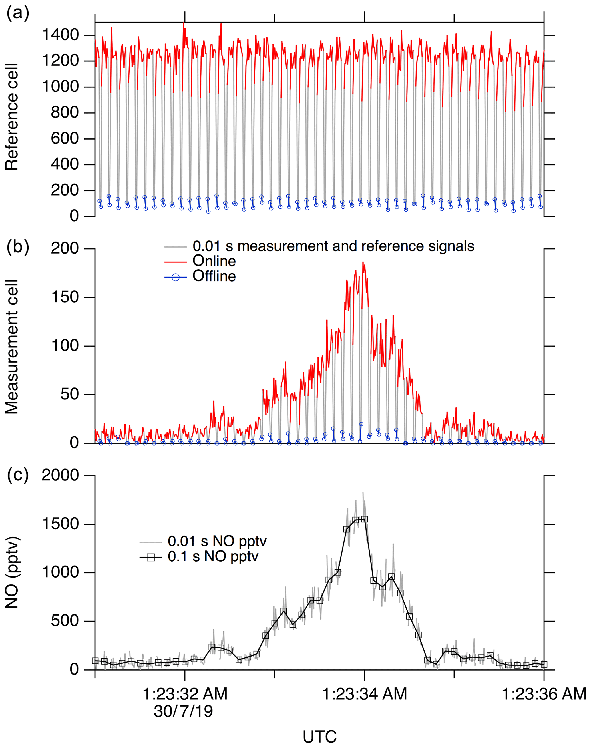
Figure 9A 5 s segment of typical data. (a) shows signal in the reference cell, and (b) shows the signal in the measurement cell. (c) shows calculated NO at 10 Hz.
The reference cell is used primarily to maintain the laser wavelength near the peak of the NO online feature. This is accomplished by continuously walking the laser wavelength around the peak (typically with a period of ∼10 s) to maintain a local maximum signal in the reference cell. A fixed differential seed laser current is maintained between the online and offline positions. For data reduction, a running boxcar average of the offline signal (typically a 1 s mean) is subtracted from the online signal in both the measurement and reference cells. Then, the online–offline difference in the measurement cell is normalized to the online–offline difference in the reference cell. This normalization accounts for the known small changes in instrument sensitivity when walking off the side of the NO peak, as well as any unintentional changes such as pressure fluctuations or small changes in the laser linewidth.
The dynamic range of the instrument is limited by the pulse-pair resolution of the photon-counting system (20 ns) and the repetition rate of the laser (320 kHz). At 85 hPa cell pressure, the lifetime of the fluorescence signal is primarily controlled by quenching and is 14 ns. Since the pulse-pair resolution is greater than the signal lifetime, the system will at most count one fluorescent photon per laser shot and therefore at very high signal levels the observed count rate will start to deviate from a linear response to the rate at which photons strike the photocathode. However, as discussed previously (Wennberg et al., 1994; Rollins et al., 2016) under the conditions of a known maximum count rate (320 kHz) the observed count rate can be corrected exactly to match the true signal rate and thereby significantly increase the dynamic range without loss of accuracy. At the present typical signal rates (∼10 counts s−1 pptv−1), errors associated with saturation would not be encountered for NO less than 100 ppbv. Figure 10 shows a typical calibration slope measured during a flight by dynamic dilution of an NO standard into the instrument inlet.
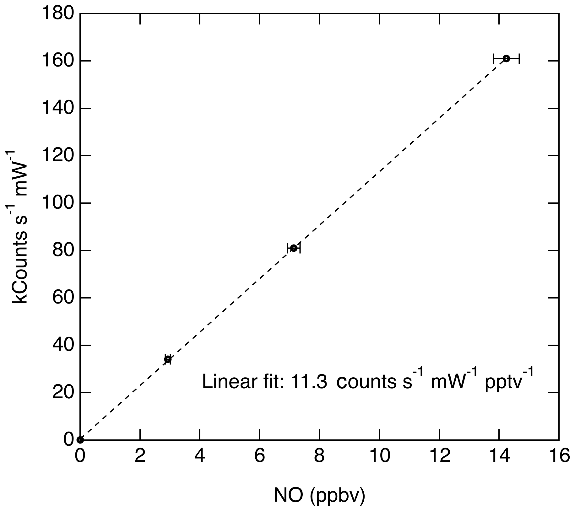
Figure 10Typical calibration data acquired during a flight when sampling a mixture of NO in zero air. Error bars indicate the 1σ uncertainty in the NO mixing ratio delivered. Statistical uncertainty in the observed signal at each point is <0.5 %.
Photolysis of other species to produce NO within the LIF cell by the probe laser could in principle pose an interference. Species known to photolyze at 215 nm producing NO include NO2 ( cm2 molecule−1), HONO ( cm2 molecule−1), and ClNO ( cm2 molecule−1). Using the estimated photon flux of 4.4×10¹⁵ photons s−1 cm−2, we calculate for the species with the largest absorption cross section (ClNO) that the photolysis rate in the probe volume of the LIF cell would be approximately 0.07 s−1. We estimate that the residence time in this volume is less than 0.01 s and therefore that less than 0.07 % of any sampled ClNO could be photolytically converted into NO. Photolysis conversion for HONO and NO2 would be respectively 10 and 100 times smaller. Such interferences are therefore negligible considering typical concentrations of these other species relative to NO in the atmosphere. A lack of significant photolytic interferences is confirmed by some of the nighttime FIREX-AQ observations when the LIF measurements show NO <0.1 % of the simultaneously measured NO2 on the aircraft.
Calibration is accomplished periodically during operation by adding typically 2–10 sccm of a 5 ppmv NO in N2 mixture to the instrument sample flow of 2500 sccm. This provides calibration mixing ratios of 4–20 ppbv. Typically, the analytical accuracy of the NIST traceable NO standard is ±1 %. The flow controller that delivers that NO to the inlet and the mass flow meter which measures total inlet flow are routinely checked against BIOS DryCals with ±1 % uncertainty each. Addition of these uncertainties in quadrature suggests that the uncertainty in the mixing ratio of NO delivered to the inlet for a single calibration point is ±2 %. For airborne measurements where water vapor mixing ratios may change rapidly and high accuracy water vapor measurements are available to correct for the NO fluorescence quantum yield, the instrument is calibrated in zero air by additionally overflowing the inlet with dry zero air (<10 ppmv water vapor).
During FIREX-AQ, the NO-LIF instrument logged more than 140 h of airborne operation over 22 flights. Typically, calibrations were performed once per hour during flights. Throughout the mission, a range of calibration coefficients were measured spanning a ±5 % range from the mean calibration coefficient, while the precision of each measurement can explain less than ±1 % of this variation. These variations in the measured calibration factors were more than was typically observed during laboratory operation, and although the calibration coefficients do not systematically vary with the environmental temperature, it is believed that the instability in sensitivity is related to the temperature of the DC-8 cabin, which varied from roughly 25 to 40 ∘C. This range may be due to apparent sensitivity changes related to temperature effects on the flow/calibration system or real changes in sensitivity due to perhaps an optical effect (e.g., etalon). The cause for the range in calibration coefficients measured in flight will be a focus of future investigation. For now, we conservatively add in quadrature this ±5 % uncertainty to the ±2 % uncertainty in the mixing ratio delivered during a calibration to arrive at a ±6 % uncertainty (1σ) in the sensitivity of the instrument in dry air.
For humidity corrections, we need to consider both the uncertainty in the water vapor measurement and in the model used to calculate the correction (i.e., Fig. 7). Typically, water vapor measurements from aircraft are known to ±10 %. By applying a 10 % uncertainty to the relationship shown in Fig. 7a for 85.4 hPa cell pressure, we derive an H2O-dependent uncertainty associated only with the uncertainty in the water vapor measurement. This relationship is roughly linear with 0 % additional uncertainty in dry air and 3 % uncertainty at 20 000 ppm H2O. For H2O greater than 10 000 ppmv, deviations between the modeled and measured effect of H2O on the fluorescence quantum yield (Fig. 7b) would add an additional 2–3 % uncertainty. This uncertainty can likely be reduced in the future by improvements in the model used to reproduce the observed effect of H2O on the NO-LIF signal.
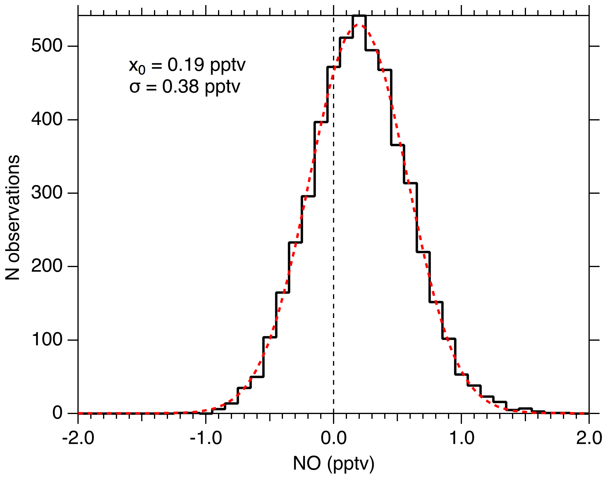
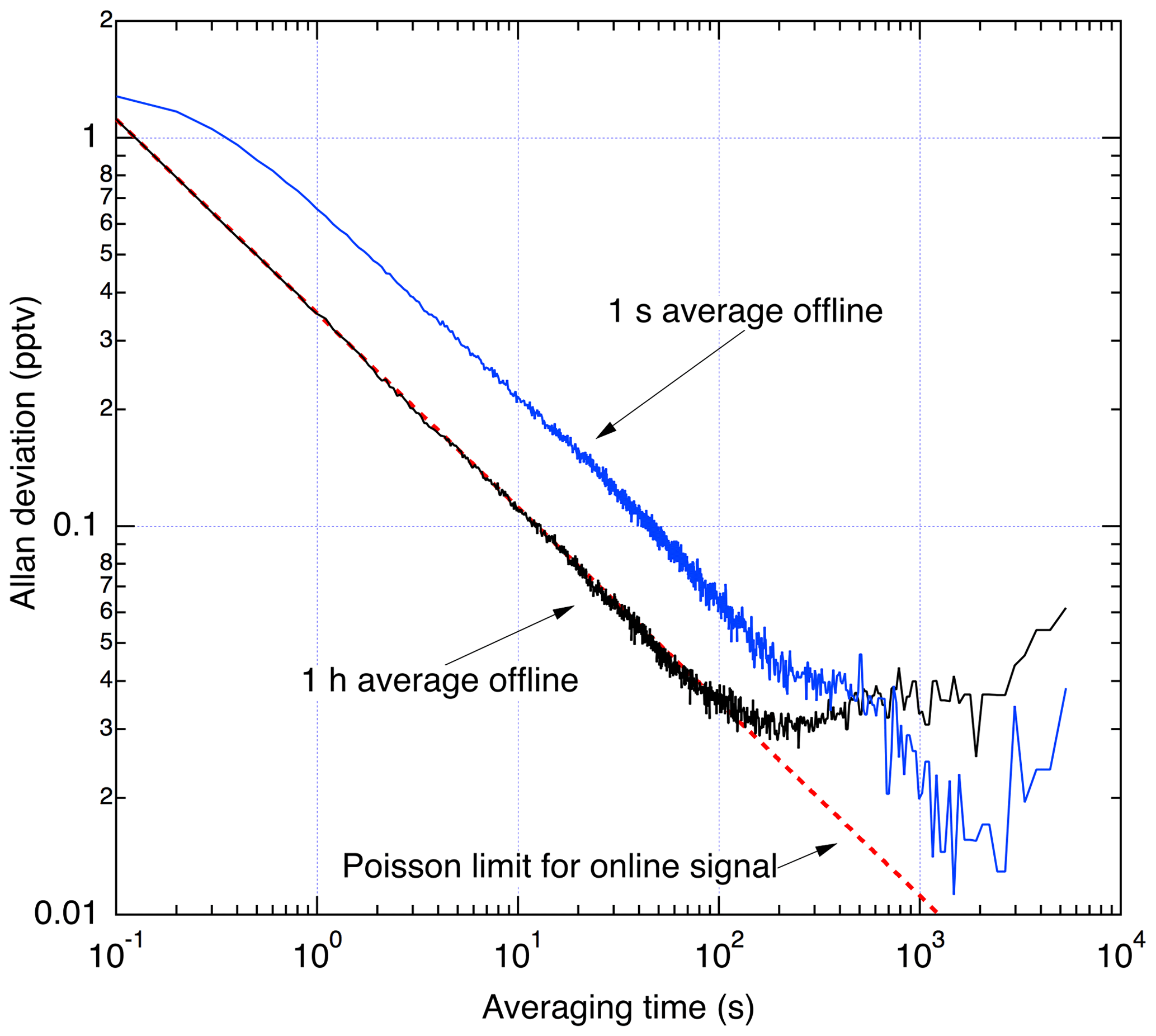
Figure 12Allan deviation analysis from 1.4 h of sampling scrubbed zero air in the laboratory.
Detection limit
The precision with very low mixing ratios of NO in the system was measured in the laboratory to test for any zero artifacts and to determine the instrumental detection limit. For these tests, the observed data were analyzed assuming that no artifact of any kind exists (i.e., the sampled NO mixing ratio is proportional to the difference between online and offline signals at all mixing ratios), and the instrumental response as determined by additions of NO standards is linear down to zero concentration. Doing this, we typically find that flowing air directly from zero-air cylinders (Praxair) into the instrument results in a measurement of 1–2 pptv NO. The observed NO was reduced to less than 0.2 pptv by flowing zero air through a potassium permanganate trap (KMnO4).
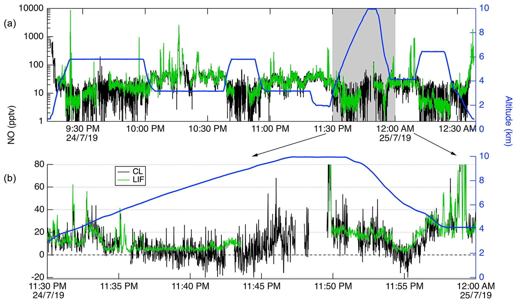
Figure 13Time series of CL (black) and LIF (green) data from a DC-8 flight on 24 July 2019. (a) shows all of the flight, with the altitude of the DC-8 plotted on the right axis in blue. (b) shows a 20 min segment expanded.
Table 1Specifications of CL and LIF instruments compared on the NASA DC-8 during FIREX-AQ. The LIF instrument is a two channel-detector, while the CL instrument has four channels, including NO, NO2, NOy, and O3. Therefore, comparisons of weight and power of the instruments should consider these differences.
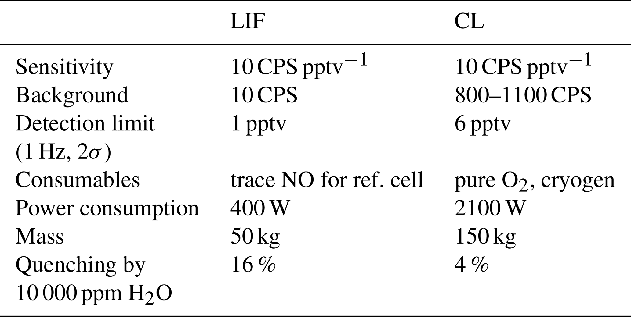
Figure 11 shows the distribution of 1 Hz NO mixing ratios measured when sampling KMnO4-scrubbed zero air for 1.4 h in the laboratory. During this period, the mean NO measured was 0.19 pptv and the noise was normally distributed with a 2σ width of 0.76 pptv. For this period, the laser power was 0.9 mW, and the NO sensitivity was 10 counts s−1 mW−1 pptv−1. The average count rate was 12 counts s−1, and thus the calculated background count rate is 10.3 counts s−1. The width of the observed mixing ratio distribution is what would be expected from a Poisson-limited distribution of the photon counts ( counts)/(10 counts mW−1 pptv mW) =0.385 pptv). This suggests that no sources other than photon-counting statistics contribute significantly to the precision near the detection limit. The calculated 2σ detection limit for a 1 s integration is therefore 0.97 pptv, and for 10 s it is 0.25 pptv. No evidence exists to suggest that the 0.19 pptv observed in the scrubbed zero air is due to anything other than NO remaining in that sample.
Figure 12 shows an Allan deviation analysis of the scrubbed zero-air sampling. During data reduction, a choice must made about what duration to use for averaging of the offline signal. Sufficiently long averaging effectively eliminates the offline signal as a source of noise, while shorter averaging assures that any changes in offline signal are completely resolved. Therefore, longer offline averaging times are only used outside of the planetary boundary layer where the NO field is changing slowly in time and is less than a few tens of pptv. To illustrate this, two analyses are shown: one where a 1 h average is used for the offline signal and another using a 1 s average offline signal. At integration times of less than 100 s, the analysis using a 1 h average of the offline signal shows that the precision is limited only by the counting statistics associated with the online signal. Instabilities in the offline signal with time constant on the order of 100–1000 s lead to lower σ using the 1 s offline average for integrations exceeding ∼10 min.
FIREX-AQ provided an excellent opportunity for evaluating the LIF instrument and for comparing it to a state-of-the-art CL instrument that was constructed and operated by NOAA. The NOAA CL instrument has significantly higher sensitivity than provided by currently available commercial CL instruments. The CL instrument was located at the front of the cabin and sampled from a probe on the port side of the aircraft. The LIF instrument was located mid-cabin, with a probe extending from the starboard side of the aircraft. The LIF instrument shared the probe described by Cazorla et al. (2015) with four other instruments, each of which sampled about 2 standard liters per minute (slpm) from the total flow of more than 20 slpm. Table 1 compares key performance and physical characteristics for the LIF and CL instruments.
Because wildfires emit significant amounts of aromatic compounds (Koss et al., 2018) which strongly absorb and fluoresce in the deep UV region, it was expected that significant enhancements and variations in the NO offline signal might be observed during FIREX-AQ. Observations during the mission, however, showed that, while fluorescence from other compounds in fires contributed to the signal, this did not significantly affect the quality of the NO measurement. For example, during typical passes through smoke on one of the flights the NO online : offline ratio decreased from 16 outside of the plume to 11.5 within the plume. This increased offline signal confirms that non-NO species in smoke do contribute to the signal but that this is typically <10 % of the signal from NO. The rapid online/offline tuning as shown in Fig. 9 eliminates significant errors due to these non-NO species.
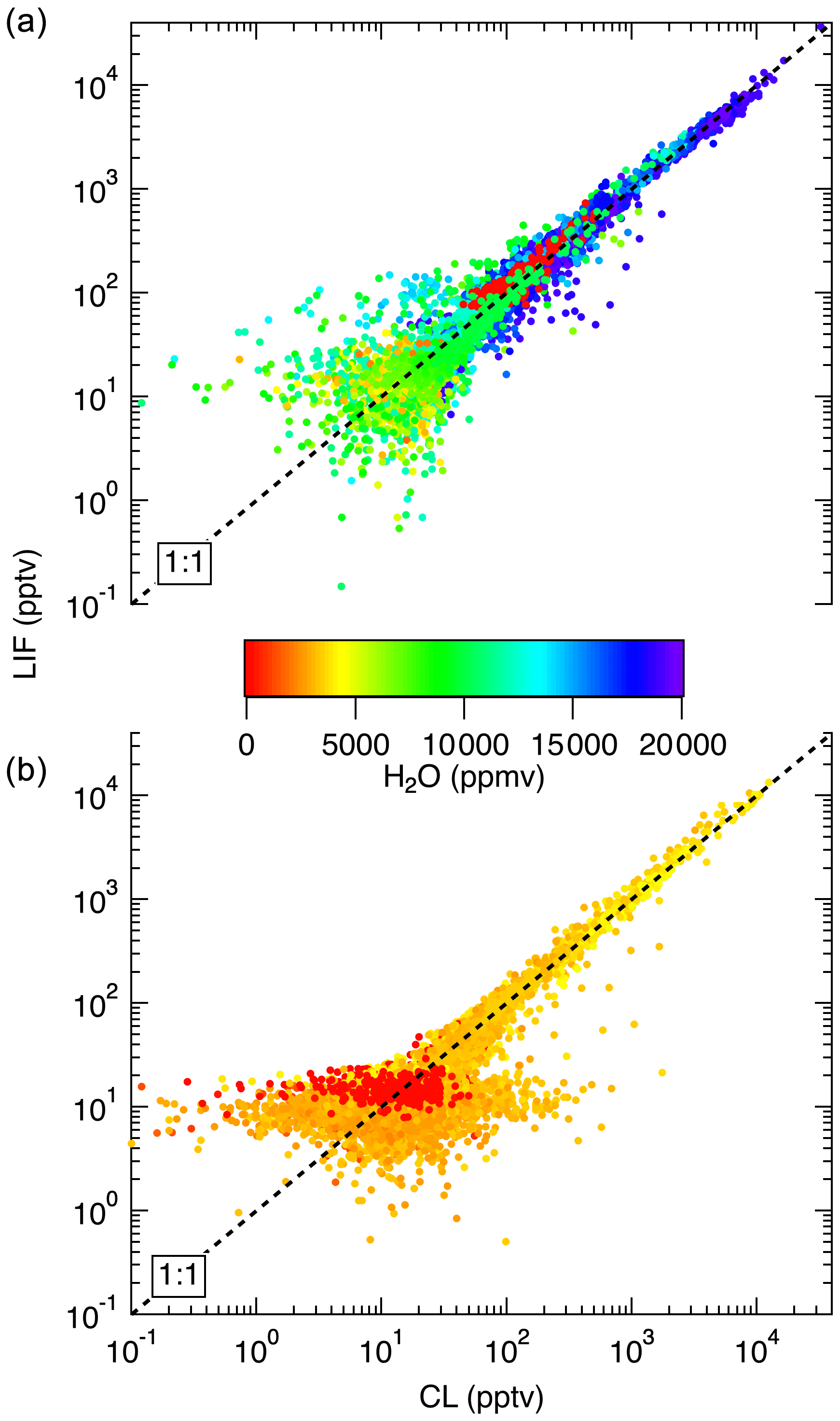
Figure 14Comparison between LIF and CL measurements from the NASA DC-8 during FIREX-AQ. (a) shows a comparison of the 1 s measurements from the flight on 22 July. This flight sampled air from the Los Angeles basin; the San Joaquin Valley; and the free troposphere transiting from Palmdale, CA, to Boise, ID. (b) compares data from a flight on 25 July, focusing on wildfire smoke sampling. Differences in LIF precision between these flights are due to unusually low laser power on the 22 July flight.
In Fig. 13, we show a time series of the 1 Hz measurements from a 3.4 h flight on 24 July 2019. This flight shows typical results from the mission. Generally, agreement between the LIF and CL instruments is excellent and we have no evidence of detectable interferences for either instrument. Small differences were sometimes observed when leaving large plumes where the NO mixing ratio would decrease by more than 1 order of magnitude over the period of 1 s. These are believed to be due to a volume in the CL instrument sample line, which is designed to match the NO2 photolysis volume in a paired channel. The lower noise of the LIF instrument is apparent primarily at mixing ratios lower than 10 pptv. Figure 14 shows scatter plots of the LIF and CL data for two flights. Panel (a) shows the comparison from a flight on 22 July 2019 during which the DC-8 sampled air throughout the California San Joaquin Valley and the Los Angeles basin, and then transited at 12.5 km altitude to Boise, ID. Panel (b) shows measurements from the flight on 25 July 2019 where the DC-8 sampled wildfire smoke while based in Boise, ID. In both figures, the data are colored by the water vapor mixing ratio measured by LGR to demonstrate that, once the data are adjusted for the measured water vapor measurements, systematic differences due to differences in water vapor are not apparent. For all data shown in Fig. 14, the regression fit slope is 0.993, indicating that the LIF-measured NO was on average 0.7 % lower than CL – a difference easily attributable to calibration uncertainties for either instrument.
CL instruments have background levels on the order of 10–100 pptv equivalent, and the background typically decreases for a number of hours after instrument operation begins. CL background also increases significantly at high altitudes and latitudes due to the unavoidable effect of cosmic rays on the large infrared-sensitive PMTs used in those instruments. These issues mean that at higher altitudes CL instrumental precision will be degraded. This can clearly be observed in Fig. 13, where the CL precision degraded significantly relative to LIF as the DC-8 climbed from 2 to 10 km altitude. Differences in data quality at low mixing ratios shown in Fig. 13 are primarily attributable to the differences in background count rates between the instruments.
A new instrument has been described for performing direct measurements of atmospheric NO using single-photon laser-induced fluorescence. The demonstrated detection limit for 10 s of integration is 0.3 pptv, and to our knowledge this is the lowest detection limit at this time resolution that has been demonstrated for an airborne atmospheric NO sensor. Besides having excellent precision, the instrument has significant practical advantages as compared to CL instruments. Consumables such as dry ice and pure oxygen are not required. The variable background in CL also means that, for accurate measurements on the order of 10 pptv to be made, frequent zero determinations must be performed, and running the instrument for a number of hours before measurements are made is desirable. In contrast, the LIF background is continuously quantified by tuning the laser offline many times each second, and the instrument does not rely on sampling of NO-free air to quantify the background of the detector. Rather, the calculated NO mixing ratio is only proportional to the difference between the online and offline signals, and sampling of very low NO zero air has shown this to be accurate to <0.2 pptv (see Sect. 6.1). For this reason, the LIF instrument requires less effort to operate and has the potential to be more accurate at low mixing ratios for typical aircraft experiments where continuous running prior to flights adds an additional experimental burden.
The LIF instrument performed well without failure and without a dedicated operator for the 22 science flights during the NASA/NOAA FIREX-AQ mission. Precision in flight was typically not as good as demonstrated in the laboratory, with the 1σ noise increasing by as much as a factor of 3. This was due to reductions in laser power (as low as 10 %) associated with the wide range of cabin air temperatures (∼25–40 ∘C) experienced on the DC-8. Future improvements in the thermal management of the laser system are expected to improve this issue. In addition, a number of possibilities exist to further improve the signal level. These include laser linewidth reduction, improved bandpass filter to collect the emission and increase the transmission at and 5, increased laser power, and increases in the geometric fluorescence collection efficiency. Altogether, we estimate that increases in signal by as much as a factor of 10 might be possible.
The one notable additional challenge associated with this LIF technique is that the signal is significantly reduced in the presence of high water vapor mixing ratios. Therefore, a fast and accurate water vapor measurement must be deployed with the NO-LIF instrument to obtain accurate NO measurements in the planetary boundary layer from aircraft. For ground-based operations where water vapor changes much more slowly, it may be acceptable to periodically calibrate the sensitivity in ambient air. For measurements in the upper troposphere and stratosphere where H2O mixing ratios are generally less than 1000 ppmv, this effect is negligible. We showed that use of the LGR measurements on the DC-8 allow us to remove any observable difference between the CL and LIF techniques associated with variable water vapor. A potential alternative strategy in the future is to use a mixture of ambient air doped with high mixing ratios of NO in the reference cell, instead of the zero-air–NO reference mixture.
The new sensor has the potential to provide high confidence in future measurements of atmospheric NO at mixing ratios of less than 10 pptv which are characteristic of much of the global remote marine boundary layer (Singh et al., 1996; Bradshaw et al., 2000). The technique can be extended to perform measurements of NO2 using selective photolytic conversion to NO (Pollack et al., 2010) or total reactive nitrogen using catalytic conversion (Kliner et al., 1997; Ryerson et al., 1999). In either case, the LIF instrument could be operated with a significantly reduced flow rate to enable the use of a smaller converter than what is typically required for use with a CL-based NO detector. In addition, the instrument has the potential to make an isotopologue-specific measurement, and lines from all of the 14N16O, 15N16O, and 14N18O isotopologues are within a range that could be reached within a single laser scan. Future efforts will focus on quantifying 15N∕14N and 18O∕16O ratios, which are unique tools for identifying sources of atmospheric NOx and diagnosing atmospheric oxidation chemistry.
The data collected on the DC-8 are available in the NASA/NOAA FIREX-AQ data archive: https://www-air.larc.nasa.gov/cgi-bin/ArcView/firexaq (last access: 20 January 2020, NASA/NOAA, 2020).
The research was designed by AWR, RSG, and SSB. Measurements were taken by AWR, PSR, TBR, JP, and IB. The paper was written by AWR with contributions from all coauthors.
The authors declare that they have no conflict of interest.
We thank the NASA DC-8 pilots and crew as well as the FIREX-AQ science team for making the NOAA/NASA FIREX-AQ mission possible. We thank the two reviewers for their insightful comments.
This paper was edited by Hendrik Fuchs and reviewed by two anonymous referees.
Bloss, W. J., Gravestock, T. J., Heard, D. E., Ingham, T., Johnson, G. P., and Lee, J. D.: Application of a compact all solid-state laser system to the in situ detection of atmospheric OH, HO2, NO and IO by laser-induced fluorescence, J. Environ. Monitor., 5, 21–28, https://doi.org/10.1039/b208714f, 2003. a, b
Bradshaw, J., Davis, D., Grodzinsky, G., Smyth, S., Newell, R., Sandholm, S., and Liu, S.: Observed distributions of nitrogen oxides in the remote free troposphere from the Nasa Global Tropospheric Experiment Programs, Rev. Geophys., 38, 61–116, https://doi.org/10.1029/1999RG900015, 2000. a
Bradshaw, J. D., Rodgers, M. O., and Davis, D. D.: Single photon laser-induced fluorescence detection of NO and SO2 for atmospheric conditions of composition and pressure, Appl. Optics, 21, 2493, https://doi.org/10.1364/AO.21.002493, 1982. a, b, c
Bradshaw, J. D., Rodgers, M. O., Sandholm, S. T., Kesheng, S., and Davis, D. D.: A two-photon laser-induced fluorescence field instrument for ground-based and airborne measurements of atmospheric NO, J. Geophys. Res., 90, 12861–12873, https://doi.org/10.1029/JD090iD07p12861, 1985. a, b, c
Cazorla, M., Wolfe, G. M., Bailey, S. A., Swanson, A. K., Arkinson, H. L., and Hanisco, T. F.: A new airborne laser-induced fluorescence instrument for in situ detection of formaldehyde throughout the troposphere and lower stratosphere, Atmos. Meas. Tech., 8, 541–552, https://doi.org/10.5194/amt-8-541-2015, 2015. a
Cohen, R. C., Perkins, K. K., Koch, L. C., Stimpfle, R. M., Wennberg, P. O., Hanisco, T. F., Lanzendorf, E. J., Bonne, G. P., Voss, P. B., Salawitch, R. J., Del Negro, L. A., Wilson, J. C., McElroy, C. T., and Bui, T. P.: Quantitative constraints on the atmospheric chemistry of nitrogen oxides: An analysis along chemical coordinates, J. Geophys. Res.-Atmos., 105, 24283–24304, https://doi.org/10.1029/2000JD900290, 2000. a
Crounse, J. D., Nielsen, L. B., Jørgensen, S., Kjaergaard, H. G., and Wennberg, P. O.: Autoxidation of organic compounds in the atmosphere, J. Phys. Chem. Lett., 4, 3513–3520, https://doi.org/10.1021/jz4019207, 2013. a
Danielak, J., Domin, U., Kepa, R., Rytel, M., and Zachwieja, M.: Reinvestigation of the Emission γ Band System () of the NO Molecule, J. Mol. Spectrosc., 181, 394–402, https://doi.org/10.1006/jmsp.1996.7181, 1997. a, b, c, d
Drummond, J. W., Volz, A., and Ehhalt, D. H.: An optimized chemiluminescence detector for tropospheric NO measurements, J. Atmos. Chem., 2, 287–306, https://doi.org/10.1007/BF00051078, 1985. a
Fahey, D. W., Kawa, S. R., Woodbridge, E. L., Tin, P., Wilson, J. C., Jonsson, H. H., Dye, J. E., Baumgardner, D., Borrmann, S., Toohey, D. W., Avallone, L. M., Proffitt, M. H., Margitan, J., Loewenstein, M., Podolske, J. R., Salawitch, R. J., Wofsy, S. C., Ko, M. K. W., Anderson, D. E., Schoeber, M. R., and Chan, K. R.: In situ measurements constraining the role of sulphate aerosols in mid-latitude ozone depletion, Nature, 363, 509–514, https://doi.org/10.1038/363509a0, 1993. a
Fittschen, C., Al Ajami, M., Batut, S., Ferracci, V., Archer-Nicholls, S., Archibald, A. T., and Schoemaecker, C.: ROOOH: a missing piece of the puzzle for OH measurements in low-NO environments?, Atmos. Chem. Phys., 19, 349–362, https://doi.org/10.5194/acp-19-349-2019, 2019. a
Gao, R. S., McLaughlin, R. J., Schein, M. E., Neuman, J. A., Ciciora, S. J., Holecek, J. C., and Fahey, D. W.: Computer-controlled Teflon flow control valve, Rev. Sci. Instrum., 70, 4732, https://doi.org/10.1063/1.1150137, 1999. a
Gao, R. S., Rosenlof, K. H., Fahey, D. W., Wennberg, P. O., Hintsa, E. J., and Hanisco, T. F.: OH in the tropical upper troposphere and its relationships to solar radiation and reactive nitrogen, J. Atmos. Chem., 71, 55–64, https://doi.org/10.1007/s10874-014-9280-2, 2014. a
Hoell, J. M., Gregory, G. L., and McDougal, D. S.: Airborne intercomparison of nitric oxide measurement techniques, J. Geophys. Res., 92, 1995–2008, https://doi.org/10.1029/JD092iD02p01995, 1987. a
Hui, M.-H. and Rice, S. A.: Comment on “Decay fluorescence from single vibronic levels of SO2”, Chem. Phys. Lett., 20, 411–412, https://doi.org/10.1016/0009-2614(73)85186-3, 1973. a
Kliner, D. A. V., Daube, B. C., Burley, J. D., and Wofsy, S. C.: Laboratory investigation of the catalytic reduction technique for measurement of atmospheric NOy, J. Geophys. Res.-Atmos., 102, 10759–10776, https://doi.org/10.1029/96JD03816, 1997. a
Koss, A. R., Sekimoto, K., Gilman, J. B., Selimovic, V., Coggon, M. M., Zarzana, K. J., Yuan, B., Lerner, B. M., Brown, S. S., Jimenez, J. L., Krechmer, J., Roberts, J. M., Warneke, C., Yokelson, R. J., and de Gouw, J.: Non-methane organic gas emissions from biomass burning: identification, quantification, and emission factors from PTR-ToF during the FIREX 2016 laboratory experiment, Atmos. Chem. Phys., 18, 3299–3319, https://doi.org/10.5194/acp-18-3299-2018, 2018. a
Laughner, J. L. and Cohen, R. C.: Direct observation of changing NOx lifetime in North American cities, Science, 366, 723–727, https://doi.org/10.1126/science.aax6832, 2019. a
Luque, J. and Crosley, D. R.: Radiative and predissociative rates for NO –5 and –3, J. Chem. Phys., 112, 9411–9416, https://doi.org/10.1063/1.481560, 2000. a
Mitscherling, C.: Selektiver Nachweis der NO-Isotopologe biologischen Ursprungs im unteren ppt-Bereich, PhD thesis, Technische Universität Braunschweig, Germany, 2009. a
Mitscherling, C., Lauenstein, J., Maul, C., Veselov, A. A., Vasyutinskii, O. S., and Gericke, K.-H.: Non-invasive and isotope-selective laser-induced fluorescence spectroscopy of nitric oxide in exhaled air, J. Breath Res., 1, 026003, https://doi.org/10.1088/1752-7155/1/2/026003, 2007. a
Mitscherling, C., Maul, C., and Gericke, K.-H.: Ultra-sensitive detection of nitric oxide isotopologues, Phys. Scripta, 80, 048122, https://doi.org/10.1088/0031-8949/80/04/048122, 2009. a
Murphy, J., Bushaw, B., and Miller, R.: Doppler-Free Two-Photon Fluorescence Excitation Spectroscopy of the A←X(1,0) Band of Nitric Oxide: Fine Structure Parameter for the (3sσ) Rydberg State of 14N16O, J. Mol. Spectrosc., 159, 217–229, https://doi.org/10.1006/jmsp.1993.1119, 1993. a
NASA/NOAA: FIREX-AQ data archive, available at: https://www-air.larc.nasa.gov/cgi-bin/ArcView/firexaq, last access: 20 January 2020. a
Nee, J., Juan, C., Hsu, J., Yang, J., and Chen, W.: The electronic quenching rates of NO(–2), Chem. Phys., 300, 85–92, https://doi.org/10.1016/j.chemphys.2004.01.014, 2004. a, b, c
Paul, P., Gray, J., Durant, J., and Thoman, J.: Collisional electronic quenching rates for NO (ν=0), Chem. Phys. Lett., 259, 508–514, https://doi.org/10.1016/0009-2614(96)00763-4, 1996. a
Pollack, I. B., Lerner, B. M., and Ryerson, T. B.: Evaluation of ultraviolet light-emitting diodes for detection of atmospheric NO2 by photolysis – chemiluminescence, J. Atmos. Chem., 65, 111–125, https://doi.org/10.1007/s10874-011-9184-3, 2010. a
Ridley, B. A. and Howlett, L. C.: An instrument for nitric oxide measurements in the stratosphere, Rev. Sci. Instrum., 45, 742, https://doi.org/10.1063/1.1686726, 1974. a
Rollins, A. W., Thornberry, T. D., Ciciora, S. J., McLaughlin, R. J., Watts, L. A., Hanisco, T. F., Baumann, E., Giorgetta, F. R., Bui, T. V., Fahey, D. W., and Gao, R.-S.: A laser-induced fluorescence instrument for aircraft measurements of sulfur dioxide in the upper troposphere and lower stratosphere, Atmos. Meas. Tech., 9, 4601–4613, https://doi.org/10.5194/amt-9-4601-2016, 2016. a, b
Ryerson, T. B., Huey, L. G., Knapp, K., Neuman, J. A., Parrish, D. D., Sueper, D. T., and Fehsenfeld, F. C.: Design and initial characterization of an inlet for gas-phase NOy measurements from aircraft, J. Geophys. Res.-Atmos., 104, 5483–5492, https://doi.org/10.1029/1998JD100087, 1999. a
Scheingraber, H. and Vidal, C. R.: Fluorescence spectroscopy and Franck–Condon-factor measurements of low-lying NO Rydberg states, J. Opt. Soc. Am. B, 2, 343, https://doi.org/10.1364/JOSAB.2.000343, 1985. a, b
Silvern, R. F., Jacob, D. J., Travis, K. R., Sherwen, T., Evans, M. J., Cohen, R. C., Laughner, J. L., Hall, S. R., Ullmann, K., Crounse, J. D., Wennberg, P. O., Peischl, J., and Pollack, I. B.: Observed NO/NO2 Ratios in the Upper Troposphere Imply Errors in NO-NO2-O3 Cycling Kinetics or an Unaccounted NOx Reservoir, Geophys. Res. Lett., 45, 4466–4474, https://doi.org/10.1029/2018GL077728, 2018. a
Singh, H. B., Herlth, D., Kolyer, R., Salas, L., Bradshaw, J. D., Sandholm, S. T., Davis, D. D., Crawford, J., Kondo, Y., Koike, M., Talbot, R., Gregory, G. L., Sachse, G. W., Browell, E., Blake, D. R., Rowland, F. S., Newell, R., Merrill, J., Heikes, B., Liu, S. C., Crutzen, P. J., and Kanakidou, M.: Reactive nitrogen and ozone over the western Pacific: Distribution, partitioning, and sources, J. Geophys. Res.-Atmos., 101, 1793–1808, https://doi.org/10.1029/95JD01029, 1996. a
Solomon, S.: Stratospheric ozone depletion: A review of concepts and history, Rev. Geophys., 37, 275–316, https://doi.org/10.1029/1999RG900008, 1999. a
Tilmes, S., Richter, J. H., Mills, M. J., Kravitz, B., MacMartin, D. G., Garcia, R. R., Kinnison, D. E., Lamarque, J. F., Tribbia, J., and Vitt, F.: Effects of Different Stratospheric SO2 Injection Altitudes on Stratospheric Chemistry and Dynamics, J. Geophys. Res.-Atmos., 123, 4654–4673, https://doi.org/10.1002/2017JD028146, 2018. a
Wennberg, P. O., Cohen, R. C., Hazen, N. L., Lapson, L. B., Allen, N. T., Hanisco, T. F., Oliver, J. F., Lanham, N. W., Demusz, J. N., and Anderson, J. G.: Aircraft-borne, laser-induced fluorescence instrument for the in situ detection of hydroxyl and hydroperoxyl radicals, Rev. Sci. Instrum., 65, 1858–1876, https://doi.org/10.1063/1.1144835, 1994. a
Western, C. M.: PGOPHER: A program for simulating rotational, vibrational and electronic spectra, J. Quant. Spectrosc. Ra., 186, 221–242, https://doi.org/10.1016/j.jqsrt.2016.04.010, 2017. a
Zhao, Y., Saunois, M., Bousquet, P., Lin, X., Berchet, A., Hegglin, M. I., Canadell, J. G., Jackson, R. B., Hauglustaine, D. A., Szopa, S., Stavert, A. R., Abraham, N. L., Archibald, A. T., Bekki, S., Deushi, M., Jöckel, P., Josse, B., Kinnison, D., Kirner, O., Marécal, V., O'Connor, F. M., Plummer, D. A., Revell, L. E., Rozanov, E., Stenke, A., Strode, S., Tilmes, S., Dlugokencky, E. J., and Zheng, B.: Inter-model comparison of global hydroxyl radical (OH) distributions and their impact on atmospheric methane over the 2000–2016 period, Atmos. Chem. Phys., 19, 13701–13723, https://doi.org/10.5194/acp-19-13701-2019, 2019. a