Total column water vapour retrieval from S-5P/TROPOMI in the visible blue spectral range

Total column water vapour has been retrieved from TROPOMI measurements in the visible blue spectral range and compared to a variety of different reference data sets for clear-sky conditions during boreal summer and winter. The retrieval consists of the common two-step DOAS approach: first the spectral analysis is performed within a linearized scheme and then the retrieved slant column densities are converted to vertical columns using an iterative scheme for the water vapour a priori profile shape, which is based on an empirical parameterization of the water vapour scale height. Moreover, a modified albedo map was used combining the OMI LER albedo and scaled MODIS albedo map. The use of the alternative albedo is especially important over regions with very low albedo and high probability of clouds like the Amazon region.

The errors of the total column water vapour (TCWV) retrieval have been theoretically estimated considering the contribution of a variety of different uncertainty sources. For observations during clear-sky conditions, over ocean surface, and at low solar zenith angles the error typically is around values of 10 %–20 %, and during cloudy-sky conditions, over land surface, and at high solar zenith angles it reaches values around 20 %–50 %.

In the framework of a validation study the retrieval demonstrates that it can well capture the global water vapour distribution: the retrieved H₂O vertical column densities (VCDs) show very good agreement with the reference data sets over ocean for boreal summer and winter whereby the modified albedo map substantially improves the retrieval's consistency to the reference data sets, in particular over tropical land masses. However, over land the retrieval underestimates the VCD by about 10 %, particularly during summertime. Our investigations show that this underestimation is likely caused by uncertainties within the surface albedo and the cloud input data: low-level clouds cause an underestimation, but for mid- to high-level clouds good agreement is found. In addition, our investigations indicate that these biases can probably be further reduced by the use of improved cloud input data. For the general purpose we recommend only using VCDs with cloud fraction <20 % and AMF >0.1, which represents a good compromise between spatial coverage and retrieval accuracy.

The TCWV retrieval can be easily applied to further satellite sensors (e.g. GOME-2 or OMI) for creating uniform, long-term measurement data sets, which is particularly interesting for climate and trend studies of water vapour.

1 Introduction

Water vapour is the most important natural greenhouse gas in the atmosphere and plays a key role in the atmospheric energy balance via radiative effects and latent heat transport (Held and Soden, 2000). Due to its high spatiotemporal variability on all atmospheric scales, accurate knowledge of the amount and distribution of water vapour is essential for numerical weather prediction and climate monitoring.

Several in situ and remote sensing measurement techniques have been developed in the past decades, enabling the observation of the water vapour distribution from platforms like radiosondes, balloons, aircrafts, and satellites. The particular absorption properties of water vapour allow for the retrieval of the water vapour content via satellites for several different spectral ranges from the radio (Kursinski et al., 1997), microwave, e.g. AMSU (Rosenkranz, 2001), thermal infrared, e.g. AIRS (Susskind et al., 2003), near and shortwave infrared, e.g. MODIS (Gao and Kaufman, 2003), MERIS (Bennartz and Fischer, 2001), and TROPOMI (Schneider et al., 2020), to the visible, e.g. GOME (Noël et al., 1999; Wagner et al., 2003; Lang et al., 2007), SCIAMACHY (Noël et al., 2004), and GOME-2 (Grossi et al., 2015).

The visible spectral range is particularly interesting for the retrieval of total column water vapour (TCWV): in contrast to the microwave range it has a similar sensitivity for the ocean and land surface, allowing for global coverage. Also, it is possible to conduct retrievals under partly-cloudy conditions and, in comparison to the thermal infrared, it has a much higher sensitivity for the near-surface layers. Furthermore, the spectral analysis is straightforward; i.e. no forward model calculations are necessary.

So far TCWV has been retrieved mostly in the visible “red” spectral range because the absorption is strongest there. However, for this spectral range the ocean surface albedo is relatively low, leading to a low sensitivity for the lowermost troposphere, where the highest water vapour concentrations occur. In addition, current and past satellite sensors can not resolve the fine absorption structure of water vapour in this spectral range, causing non-linear absorption effects (e.g. saturation) which have to be accounted for in post-processing. Thus, Wagner et al. (2013) suggested applying retrievals in the “blue” spectral range (around 442 nm) where the absorption is much weaker than in the red, making the retrieval problem quasi-linear. In addition, the ocean surface albedo is much higher, leading to a higher sensitivity of the near-surface layers. The first operational analyses of a similar approach have been performed by Wang et al. (2019) for measurements of the Ozone Monitoring Instrument (OMI, Levelt et al., 2006).

In October 2017 the TROPOspheric Monitoring Instrument (TROPOMI, Veefkind et al., 2012) onboard ESA's Sentinel-5 Precursor (S-5P) satellite was launched in a Sun-synchronous polar orbit with an Equator crossing time of 13:30 LT (local time). TROPOMI is a UV-Vis-NIR push-broom spectrometer and consists of 450 detectors/rows covering a swath width of 2600 km. The outstanding property of TROPOMI is that its spectral bands in the visible combine a high signal-to-noise ratio with an unprecedented spatial resolution of 3.5×7.5 km² (and 3.5×5.6 km² since August 2019; Rozemeijer and Kleipool, 2019) at nadir, which allows for the performance of spectral analyses at a never seen before accuracy even on small spatial scales.

In this paper we introduce a TCWV retrieval based on the spectral analysis approach of Wagner et al. (2013) to S-5P/TROPOMI observations. The paper is organized as follows: in Sect. 2 we give an overview of the retrieval describing general retrieval principles and presenting the retrieval setup. In Sect. 3 we present an empirical parameterization of the a priori water vapour profile shape and an iterative scheme making use of the relation between the water vapour profile shape and TCWV. In Sect. 4 we evaluate different input albedo products and in Sect. 5 we perform a detailed uncertainty analysis including a variety of different error sources. In Sect. 6 we present first TCWV results retrieved from TROPOMI measurements and perform a validation study using data sets from satellites, ground-based measurements, and reanalysis models as reference. In Sect. 7 we draw conclusions and summarize the outcomes of our investigations.

2 Retrieval principles

2.1 Wavelength calibration and spectral analysis

In a first step the wavelength alignment of the daily measured irradiance is calibrated for each of the 450 TROPOMI detectors/rows via a non-linear least-squares fit in intensity space using the solar spectrum from Kurucz et al. (1984) as reference. Simultaneously, the instrumental spectral response function (ISRF) is approximated assuming an asymmetric Super-Gaussian following the definition of Beirle et al. (2017):

$$\begin{array}{}\text{(1)}& S_{\mathrm{asym}}\left(x\right)=\left\{\begin{array}{ll}\exp \left(-{\left|\frac{x}{w-a_w}\right|}^k\right)& \text{for }x\le \mathrm{0},\\ \exp \left(-{\left|\frac{x}{w+a_w}\right|}^k\right)& \text{for }x>\mathrm{0}.\end{array}\right.\end{array}$$

Next, we perform a spectral analysis using the differential optical absorption spectroscopy (DOAS; Platt and Stutz, 2008) scheme in which the attenuation along the light path is calculated via the Beer–Lambert law in optical depth space:

$$\begin{array}{}\text{(2)}& \ln \left({\displaystyle \frac{I}{I_{\mathrm{0}}}}\right)=\mathit{\tau }\approx -\sum _i{\mathit{\sigma }}_i\left(\mathit{\lambda }\right)\cdot {\mathrm{SCD}}_i+\mathrm{\Phi },\end{array}$$

where i denotes the index of a trace gas of interest, σ_i(λ) its respective absorption cross section, ${\mathrm{SCD}}_i={\int }_s{c}_i\mathrm{d}s$ its concentration integrated along the light path s (the so-called slant column density), and Φ a closure polynomial accounting for Mie and Rayleigh scattering as well as low-frequency contributions.

Table 1 summarizes the fit setup of the retrieval's spectral analysis. The retrieval's fit window ranges from 430 to 450 nm and accounts for molecular absorption by water vapour (HITRAN 2008, Rothman et al., 2009), NO₂ at 220 K (Vandaele et al., 1998), ozone (Serdyuchenko et al., 2014), and the O₂–O₂ dimer (Thalman and Volkamer, 2013). In order to account for the Ring effect we include two Ring spectra (Wagner et al., 2009), and for Φ we use a fifth-order polynomial. Furthermore, we include pseudo-absorbers accounting for intensity offset, for shift and stretch effects (Beirle et al., 2013), and for ISRF changes along the orbit (Beirle et al., 2017) for ISRF parameters w and k in Eq. (1). All molecular absorption cross sections are convolved with the ISRF of the corresponding TROPOMI row/detector determined during the calibration process.

(Rothman et al., 2009)(Vandaele et al., 1998)(Serdyuchenko et al., 2014)(Thalman and Volkamer, 2013)(Beirle et al., 2013)(Beirle et al., 2017)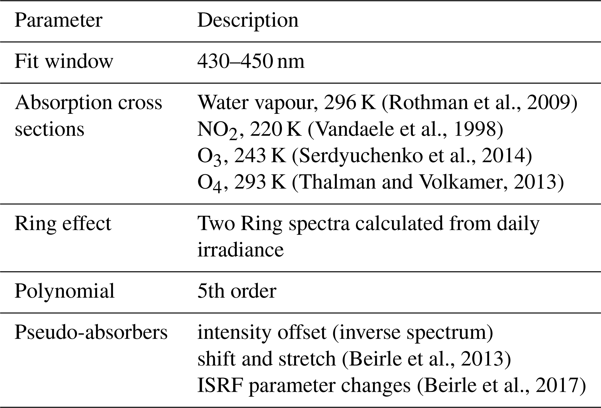

Table 1 DOAS fit settings for the H₂O slant column retrievals.

The molecular absorption by water vapour within our fit window is relatively weak, and hence the modelled line lists vary systematically from HITRAN 2008 to HITRAN 2012 (Rothman et al., 2013) and to HITRAN 2016 (Gordon et al., 2017). Thus, the choice of line list is afflicted by a high degree of uncertainty. Lampel et al. (2015) found out that HITRAN 2012 underestimates the water vapour concentration derived from long-path DOAS observations by approximately 10 % and that the previous version, HITRAN 2008, agrees better with the reference measurements. Further long-path DOAS measurements taken during the CINDI-2 campaign also confirm the findings from Lampel et al. (2015) (see Appendix B for more details). Hence, combining the findings from Lampel et al. (2015) and Wang et al. (2019), we conclude that HITRAN 2008 fits best our needs and is superior to the most recent version of the HITRAN line lists (HITRAN 2016).

Due to the high daily data volume of the TROPOMI L1B radiances, the execution of a non-linear fit without high-performance infrastructure is demanding in computation time. For instance, TROPOMI's UVIS Band 4, which covers the spectral range of 400–499 nm, generates about 40 GB every day. Therefore, we implemented a weighted linear least-squares fit for our retrieval, in which the weights are the fractional coverage of the spectral pixel within the fit window (details in Appendix A). This weighting of the outermost pixels of the fit window avoids “jumps” of pixels included in the DOAS fit, as they would occur for a fixed fit window due to the changing pixel-to-wavelength mapping across-track. Thus, across-track “stripes” in the SCDs are avoided. According to Beirle et al. (2013) the computational speed increases by 3 orders of magnitude by going from non-linear to linear fits for their MATLAB routine (see Table 3 in their paper).

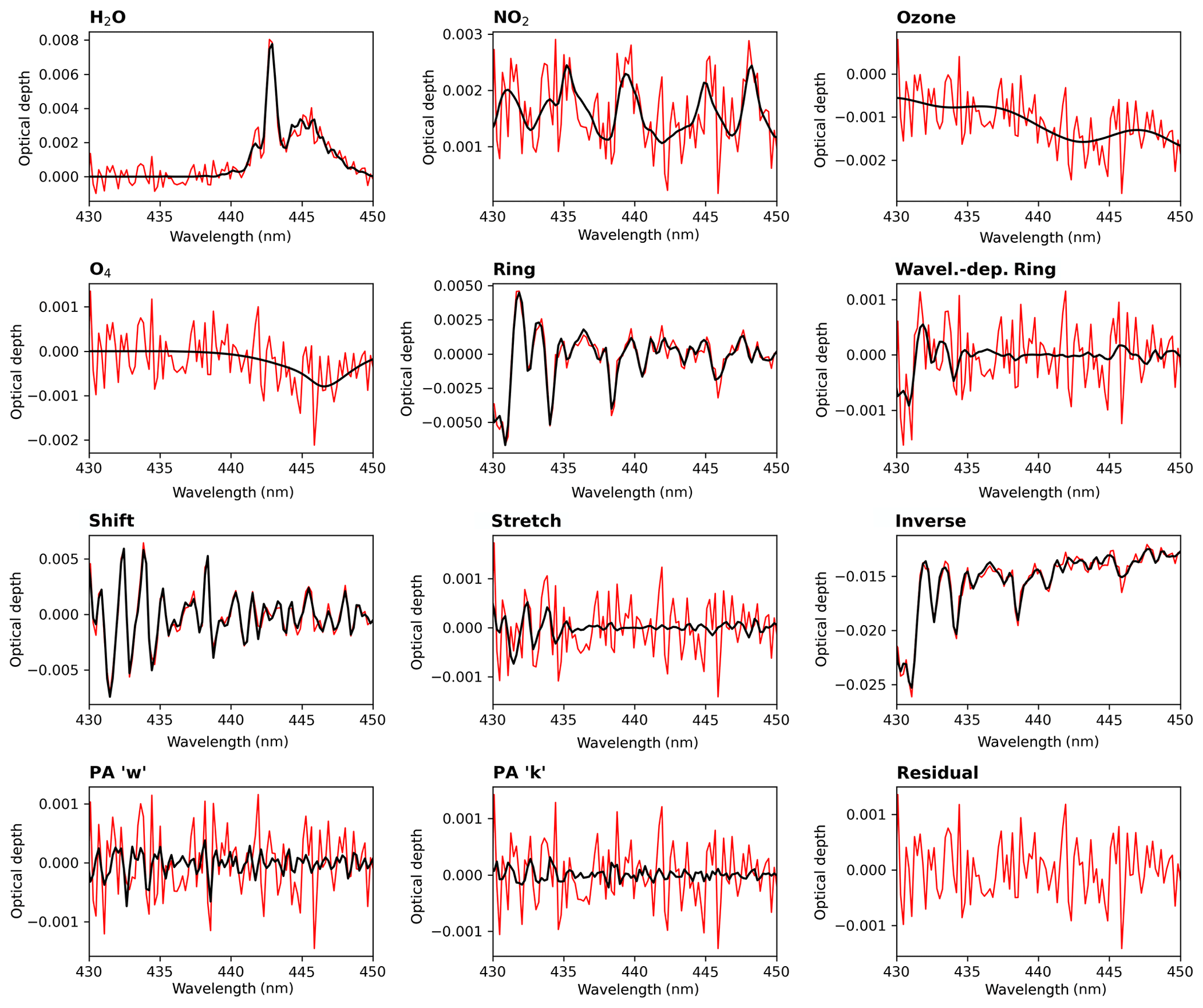
Figure 1 Example of a typical spectral analysis of a TROPOMI measurement spectrum (rms: 0.5 ‰, orbit: 6930, −7.41^∘ N, −111.97^∘ E). The black line indicates the fit result for the respective trace gas and the red line indicates the residual spectrum and residual noise for each constituent.

Figure 1 illustrates a typical example of such a spectral analysis of a TROPOMI measurement spectrum in which the absorption structures of water vapour, NO₂, and the Ring effect can be well identified and the residual spectrum shows a mainly noisy structure. Figure 2 depicts the distribution of the H₂O SCD from one TROPOMI orbit (orbit number 6930) on 13 February 2019. It demonstrates that the TROPOMI retrieval is able to capture the meso- to macro-scale water vapour patterns like convective updrafts in the tropics and atmospheric rivers in the midlatitudes, whereby the small H₂O SCD values in the tropics are caused by cloud shielding.

Figure 2 H₂O SCD distribution retrieved from TROPOMI measurements (orbit: 6930) on 13 February 2019 during an atmospheric river event at the western US coast.

2.2 Vertical column density conversion and Box-AMF simulations

To convert the slant column density to a vertical column density (VCD), we apply the so-called air-mass factor (AMF):

$$\begin{array}{}\text{(3)}& \mathrm{VCD}={\displaystyle \frac{\mathrm{SCD}}{\mathrm{AMF}}}.\end{array}$$

The air-mass factor accounts for the non-trivial effects of the atmospheric radiative transfer and is usually based on radiative transfer model (RTM) simulations. In our case we used the 3D Monte Carlo RTM McArtim (Deutschmann et al., 2011) and performed simulations at a wavelength of 442 nm for different retrieval scenarios (summarized in Table 2) assuming an aerosol-free atmosphere. These simulations yield a Jacobian vector $\mathit{J}=\frac{\partial \ln I}{\partial \mathit{\mu }}$ (with the absorption coefficient μ and the simulated intensity I at TOA normalized by the solar spectrum I₀) defined at each grid box k. The altitude-dependent AMFs (BAMF) can then be calculated according to the formula

$$\begin{array}{}\text{(4)}& {\mathrm{BAMF}}_k=-{\displaystyle \frac{{\mathit{J}}_k}{I\mathrm{\Delta }h}},\end{array}$$

with the box thickness Δh. These BAMF profiles have to be combined with the partial vertical columns c_k of an a priori water vapour profile:

$$\begin{array}{}\text{(5)}& \mathrm{AMF}={\displaystyle \frac{{\sum }_k{\mathrm{BAMF}}_k\cdot c_k}{{\sum }_k{c}_k}},\end{array}$$

with ${\sum }_k{c}_k=\mathrm{VCD}$. For the case of a cloud-contaminated pixel we assume that the cloud is a Lambertian reflector with an albedo of 80 % and use the cloud top height as surface altitude input for the AMF. Under the assumption of the independent pixel approximation, the resulting cloud-affected AMF can then be calculated as a linear combination of the AMF for a clear-sky scenario and the AMF for a cloudy-sky scenario weighted by the respective simulated intensities I and the effective cloud fractions ζ as follows:

$$\begin{array}{}\text{(6)}& \mathrm{AMF}={\displaystyle \frac{\left(\mathrm{1}-\mathit{\zeta }\right)I_{\mathrm{clear}}{\mathrm{AMF}}_{\mathrm{clear}}+\mathit{\zeta }\cdot I_{\mathrm{cloud}}{\mathrm{AMF}}_{\mathrm{cloud}}}{\left(\mathrm{1}-\mathit{\zeta }\right)I_{\mathrm{clear}}+\mathit{\zeta }\cdot I_{\mathrm{cloud}}}}.\end{array}$$

Figure 3 depicts typical examples of BAMF profiles for different clear- and cloudy-sky scenarios. The AMFs for the cloudy-sky scenarios were calculated assuming a surface albedo of 7 % and an effective cloud fraction of 20 %. For the clear-sky scenario (panel a) the sensitivity decreases towards the surface. For the cloudy-sky scenarios (panel b) the BAMF profiles slightly increase towards the (bright) cloud top surface of the respective scenario. Below the cloud, the sensitivity is 0, because the atmosphere is shielded. Since high clouds shield large fractions of the atmosphere and hence also of the water vapour column below the cloud (see the black dashed curve), the AMF has to be corrected correspondingly and thus decreases for increasing cloud top heights.

Table 2 Parameter list and nodes for the BAMF profile simulations.

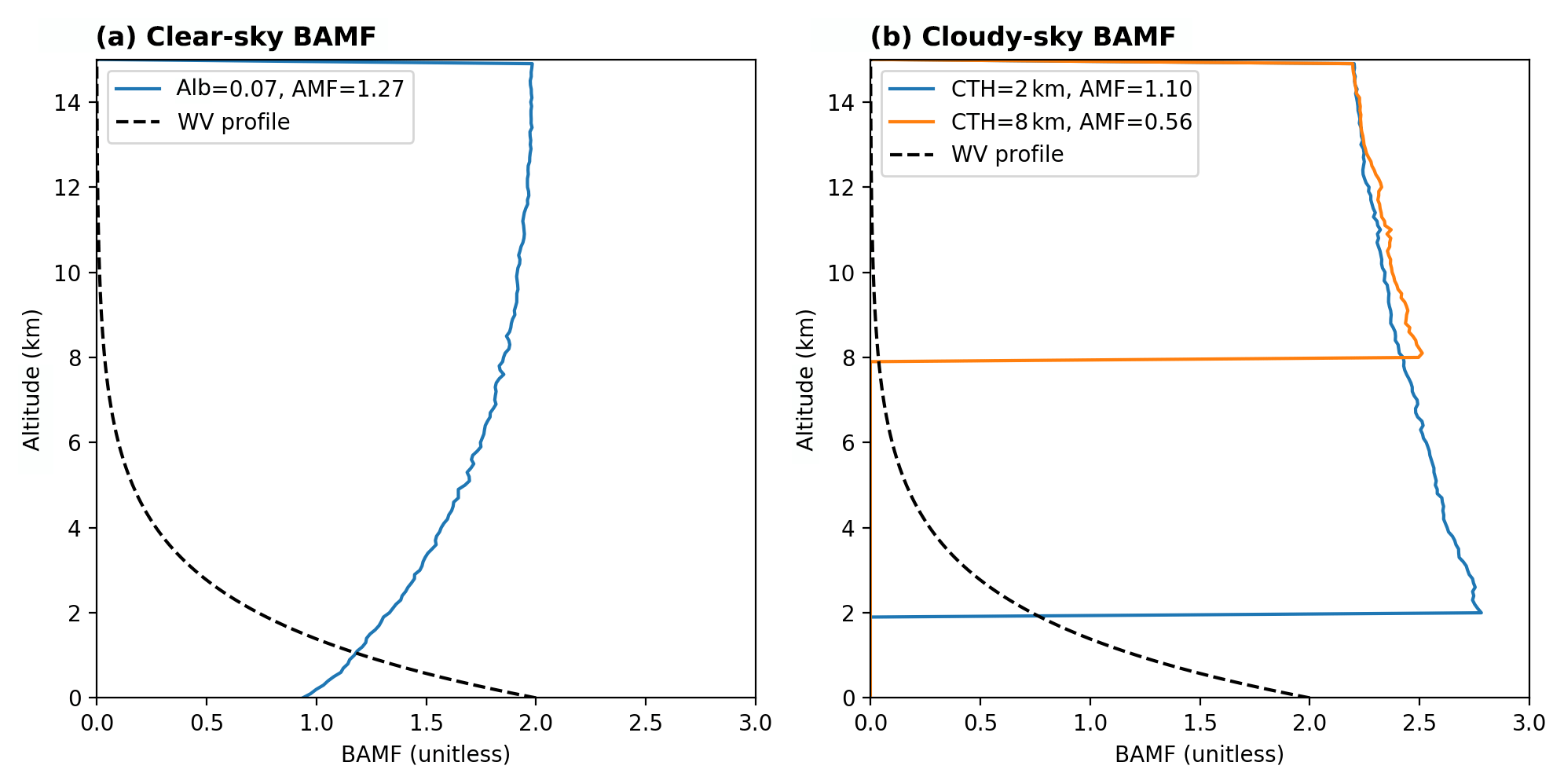
Figure 3 Examples of typical BAMF profiles for different observation scenarios under clear- (a) and cloudy-sky (b) conditions. For all profiles we assume a solar zenith angle of 0^∘, a line-of-sight angle of −90^∘, and a solar relative azimuth angle of 0^∘. For the clear-sky case the BAMF profile is illustrated for a surface albedo of 7 %. For the cloudy-sky cases the profiles are depicted as cloud top heights of 2 and 8 km and the respective AMFs are calculated assuming a surface albedo of 7 % and an effective cloud fraction of 20 %. The black dashed lines indicate relative water vapour concentrations with a scale height of 2 km.

3 A priori water vapour profile shape

As described in Sect. 2.2 and Eq. (5), knowledge of the a priori water vapour profile shape is necessary for accurate calculations of the AMF from the BAMF profile. However, simply assuming the same a priori profile shape for the whole globe might cause biases because it can not account for the atmospheric variability of water vapour, such as latitudinal variation, seasonal cycles, or different profile shapes over maritime and continental regions due to different water vapour sources (e.g. evapotranspiration by plants). Also, simply using profiles from numerical weather models is not uncritical: for instance, Wang et al. (2019) found out that their calculated AMF changes strongly, depending on which reanalysis model data they were using.

Weaver and Ramanathan (1995) approximated the water vapour profile by an exponential decay with altitude:

$$\begin{array}{}\text{(7)}& n_{\mathrm{v}}\left(z\right)=n_{\mathrm{0}}{e}^{-z/H_{\mathrm{v}}},\end{array}$$

where H_v is the scale height of water vapour, which they defined as

$$\begin{array}{}\text{(8)}& H_{\mathrm{v}}={\displaystyle \frac{R_{\mathrm{v}}{〈T〉}^{\mathrm{2}}}{L〈\mathrm{\Gamma }〉}},\end{array}$$

where 〈T〉 denotes the mean air temperature within an atmospheric column, 〈Γ〉 the mean lapse rate within the same atmospheric column, R_v the gas constant of water vapour, and L the specific latent heat. However, this definition requires knowledge of the mean air temperature and/or the lapse rate and that the relative humidity is constant with altitude. The former can be only estimated using numerical weather models and the latter is very unlikely to occur in the atmosphere.

Thus, we investigate to find an empirical parameterization of the scale height and thereby focus on its dependency on the H₂O VCD and the aforementioned atmospheric variabilities, i.e. dependencies of latitude, seasonal cycle, and surface properties (such as vegetation effects).

We proceed as follows: first, we evaluate how well the method used to calculate the water vapour scale height can reproduce the COSMIC profiles via an AMF comparison. Then we examine how the scale height can be parameterized globally and investigate for a parameterization over ocean and land separately. Finally, we implement the parameterization in an iterative retrieval scheme and evaluate the new estimates of the H₂O VCD.

3.1 COSMIC water vapour profiles

For our investigations we use profile data retrieved from measurements of the Constellation Observing System for Meteorology, Ionosphere, and Climate (COSMIC, Anthes et al., 2008) program provided by the Radio Occultation Meteorology Satellite Application Facility (ROMSAF). The COSMIC data are based on the GPS radio occultation (RO) technique, which provides high-resolution vertical profiles of bending angles (Hajj et al., 2002) that can be used to retrieve the atmospheric refractivity. Since the atmospheric refractivity is dependent on the air pressure, the air temperature, and the water vapour pressure (Smith and Weintraub, 1953), GPS RO allows for the retrieval of profile information under all-weather conditions with a high vertical resolution of approximately 100 m in the lower troposphere up to 1 km in the stratosphere (Anthes, 2011) and an accuracy of around 1 g kg⁻¹ (Heise et al., 2006; Ho et al., 2010b) while having an almost uniform global distribution (Ho et al., 2010a).

The ROMSAF profiles have been retrieved via a 1D-VAR scheme within a reprocessing initiative for creating climate data record (CDR) v1.0. Given the strict product requirements and the validation studies with ERA-Interim and radiosondes (Nielsen et al., 2018), biases associated with using COSMIC should be of secondary order.

We use data retrieved between 2013 and 2016, which accumulates to approximately 1.6×10⁶ profiles.

3.2 Calculation of scale height

For the calculation of the scale height we high-sample the COSMIC profile to a 100 m grid up to 14 km, or rather only consider profile data below 150 hPa (close to the tropopause height). Then we sum up all the partial columns of the COSMIC profile data from the ground up to a (scale) height H_sum where the H₂O VCD reaches $\mathrm{1}-\frac{\mathrm{1}}{e}$:

$$\begin{array}{}\text{(9)}& {\displaystyle \frac{{\int }_{\mathrm{0}}^{H_{\mathrm{sum}}}n\left(z\right)\mathrm{d}z}{{\int }_{\mathrm{0}}^{\mathrm{TOA}}n\left(z\right)\mathrm{d}z}}>\mathrm{1}-{\displaystyle \frac{\mathrm{1}}{e}}\approx \mathrm{63}\mathit{\%}.\end{array}$$

To evaluate this scale height approach, we performed a synthetic study in which we compared AMFs calculated for the original COSMIC water vapour profile measurements with AMFs for an exponential profile using the corresponding calculated scale height H_sum. For the simulation of the BAMF profiles we assume an albedo of 7 %, which is a representative value for the ocean surface albedo (Tilstra et al., 2017). The solar zenith angle is calculated for the location of the COSMIC profile assuming an hour angle of 90^∘, and the line-of-sight angles are prescribed for −90, −70, and −50^∘.

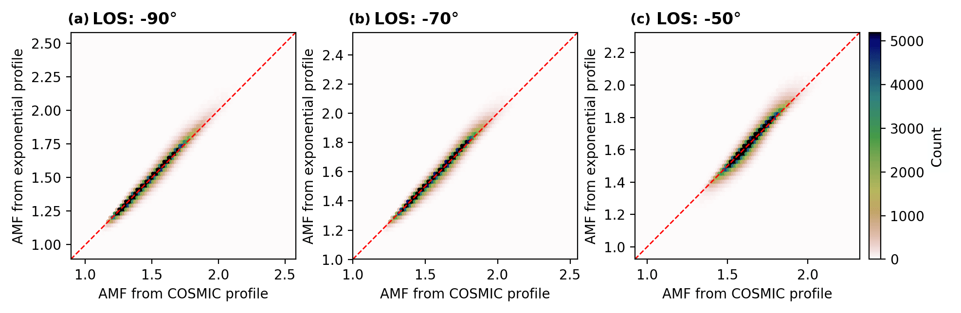
Figure 4 2D histograms comparing synthetic AMFs (calculated via the sum method) for different line-of-sight angles (a: −90^∘, b: −70^∘, and c: −50^∘) assuming clear-sky conditions. The colour depicts the number of observations within one defined bin of the 2D histogram and the red dashed line represents the 1-to-1 diagonal.

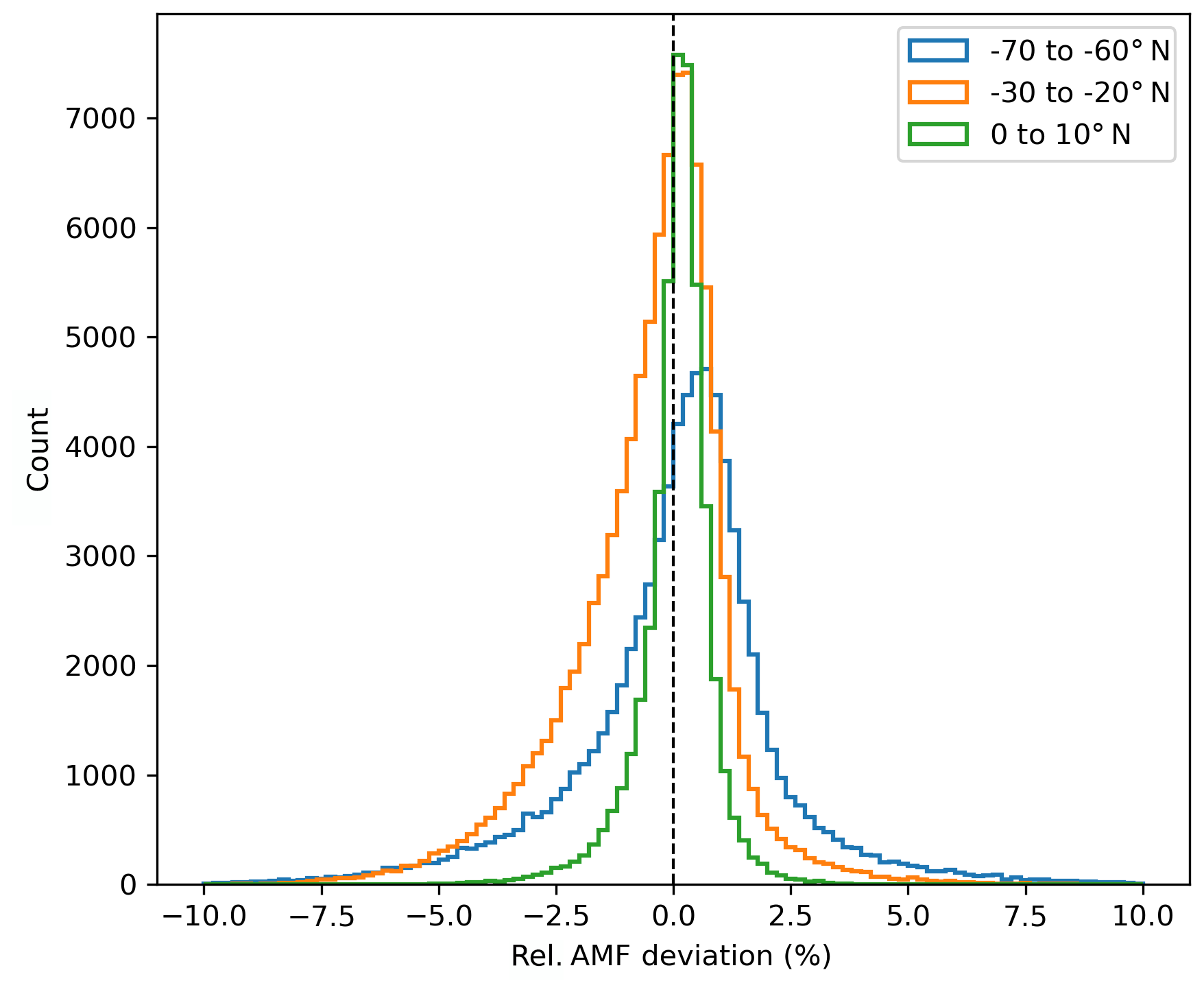
Figure 5 Histogram of the relative deviation of the calculated synthetic AMFs between the exponential profile and COSMIC profile for selected latitude bins (0 to 10, −30 to −20, and −70 to −60^∘ N) assuming clear-sky conditions and nadir-viewing geometry.

The results of the intercomparison are given in Fig. 4. The 2D histograms reveal that the AMFs derived with the exponential profile agree well with the AMFs calculated directly from the COSMIC profiles, indicating that the chosen method can well reproduce the shapes of the COSMIC profiles. This good agreement can also be observed in the histograms of Fig. 5, which illustrate distributions of relative deviation between the AMFs for selected latitude bins. These distributions have a sharp shape and peak around values of 0 %, indicating that the AMFs from the exponential shape are almost unbiased to the reference AMFs. In addition, Fig. S1 in the Supplement shows exemplary profiles for cases of good and bad agreement with the reference AMFs for the same selected latitude bins as in Fig. 5. In general, bad agreement (left column) occurs for profile shapes in which a sharp gradient is observed in the lower troposphere and from that quasi-constant values with altitude. Such profiles usually occur when a moist boundary layer is topped by a dry free atmosphere. Nevertheless, the maximal absolute relative AMF deviations only have values around 15 %. In contrast, good agreement (right column) is found for profile shapes following an exponential decay with altitude, which indicates a well-mixed troposphere.

The results of the intercomparison for prescribed cloudy-sky conditions and nadir-viewing geometry are illustrated in Fig. S2, in which the panels show histograms of the relative AMF deviation for the same selected latitude bins as in Fig. 5 but for different cloud fraction (10 %, 20 % and 50 %; left to right column) and cloud top height (1, 2, and 5 km; top to bottom rows) scenarios. For a cloud top height of 1 km the AMFs calculated from the exponential profiles are generally biased negative for all cloud fractions, in particular for the latitude bin of −30 to −20^∘ N. However, for higher clouds the AMFs agree well with the reference AMFs for almost all cloud scenarios except the extreme case with a cloud fraction of 50 % and a cloud top height of 5 km or more.

Alternative methods for calculating the scale height yielded systematic overestimations of the AMF for clear-sky conditions (Fig. C1) and higher scatter within the AMF for cloudy-sky conditions (Fig. S8) in comparison to the sum method, as shown in detail in Appendix C.

3.3 Parameterization of scale height

Figure 6 depicts the distribution of the calculated COSMIC scale height H_sum against the COSMIC TCWV for boreal summer over ocean for latitude bins of 10^∘. The regression fits (solid red lines) are based on orthogonal distance regression (ODR) using the “scipy.odr” package built on ODRPACK (Boggs et al., 1992). For low latitudes (tropics and subtropics) the scale height shows a high linear correlation with the H₂O VCD, with slopes around 0.04 and Pearson correlation coefficients R of 70 % and above. In contrast, for high latitudes the slope increases up to 0.1, and the scatter also increases distinctively; i.e. the correlation coefficient only reaches values of around 0.3 in the polar regions. This decrease in linear agreement is likely caused by the higher atmospheric variability due to higher atmospheric dynamics in the midlatitudes. Also, the uncertainty is higher in the COSMIC profile because a drier atmosphere leads to a smaller sensitivity of the COSMIC profile retrieval to water vapour concentrations (compare Kursinski et al., 1997).

Figure 6 2D histograms depicting the relation between calculated scale height and TCWV from COSMIC profiles for boreal summer (June, July, and August) only over ocean summarized in 10^∘ latitude bins. Only latitude bins with a sample size of 1500 data points are illustrated. The colour indicates the relative share of total points within one bin of the histogram and the red line indicates the fit results of the orthogonal distance regression with detailed results in the legend of each subplot. In addition the Pearson correlation coefficient for each data set is given in the title of each subplot.

Figure 7 Same as Fig.6 but for data over land.

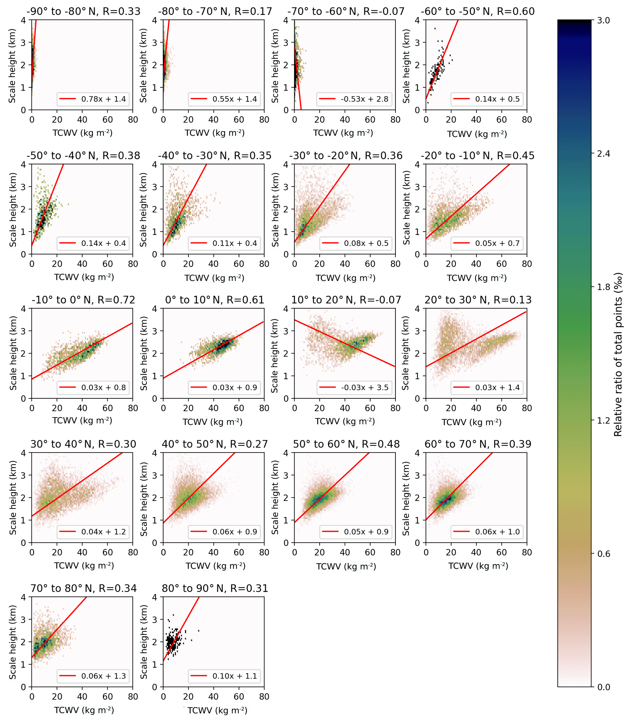
Figure 7 illustrates the same panels as Fig. 6 but for data over land. In general, the scatter for all latitude bins has increased distinctively, resulting in an inferior linear agreement between the H₂O VCD and the scale height compared to the data over ocean, especially for deserts and northern polar regions. Fortunately, the surface albedo of these regions is usually high, and thus the AMF is less dependent on the a priori profile shape. In addition, these regions are governed by an arid climate, and thus the retrieved H₂O VCDs are expected to be small. Correspondingly, the absolute H₂O VCD errors due to uncertainties in the AMF are still relatively small.

In the following we investigate a parameterization of the scale height with respect to H₂O VCD, latitude, and season for ocean and land separately. To distinguish between ocean and land surface, we use a land–sea mask derived from GSHHS coastline data (Wessel and Smith, 1996).

Figure 8 Summary of the results of the ODR fit between COSMIC scale height and COSMIC TCWV as a function of latitude and month for data over ocean. Panel (a) illustrates the fitted slopes and panel (b) the corresponding fitted intercepts whereby the coloured points represent the fit results and the lines represent the approximations for α(θ,t) and β(θ,t) for each month.

3.3.1 Ocean

The regression line parameters of the ODR fit results between COSMIC TCWV and COSMIC scale height for each latitude bin for each month for data over ocean are illustrated in Fig. 8. The values for the fitted slopes (Fig. 8a) indicate a quadratic dependency with latitude and reveal a seasonal shift towards higher latitudes during July, August, and September. Also, the values for the fitted intercept vary with latitude and season.

Thus, the scale height over ocean H_ocean can be approximated as follows:

$$\begin{array}{}\text{(10)}& H_{\mathrm{ocean}}(\mathrm{VCD},\mathit{\theta },t)=\mathit{\alpha }(\mathit{\theta },t)\cdot \mathrm{VCD}+\mathit{\beta }(\mathit{\theta },t),\end{array}$$

with

$$\begin{array}{}\text{(11)}& \begin{array}{rl}& \mathit{\alpha }(\mathit{\theta },t)=a_{\mathrm{0}}\left(t\right)+a_{\mathrm{1}}\left(t\right)\cdot \mathit{\theta }+a_{\mathrm{2}}\left(t\right)\cdot {\mathit{\theta }}^{\mathrm{2}},\\ & \mathit{\beta }(\mathit{\theta },t)=b_{\mathrm{0}}\left(t\right)+b_{\mathrm{1}}\left(t\right)\cdot \mathit{\theta }+b_{\mathrm{2}}\left(t\right)\cdot \left|\mathit{\theta }-{\mathit{\theta }}_{\mathrm{0}}\left(t\right)\right|,\end{array}\end{array}$$

with the latitude θ and the day of year t. The annual variation of the function parameters a_i, b_i, and θ₀ from Eq. (11) fitted for the monthly data sets (illustrated in Fig. 8) is depicted in Fig. S9. Most function parameters reveal an annual and semi-annual cycle over the year. Hence, these function parameters can be approximated by a superposition of two simple cosine functions with prescribed frequencies:

$$\begin{array}{}\text{(12)}& a_i\left(t\right)=a_{i\mathrm{1}}\cdot \cos \left(a_{i\mathrm{2}}+\mathit{\omega }t\right)+a_{i\mathrm{3}}\cdot \cos \left(a_{i\mathrm{4}}+\mathrm{2}\mathit{\omega }t\right)+a_{i\mathrm{5}},\end{array}$$

with t as the day of year and $\mathit{\omega }=\frac{\mathrm{2}\mathit{\pi }}{\mathrm{365}}$. Such functions have also been fitted and illustrated for the monthly data in Fig. S9 (solid orange lines), whereby we assumed that the day of year representing the month is the first day of the month. For most function parameters the fits coincide well with the data points, and in the cases of suboptimal fit results the annual variation of the data is relatively small, indicating that our choice of parameterization is valid.

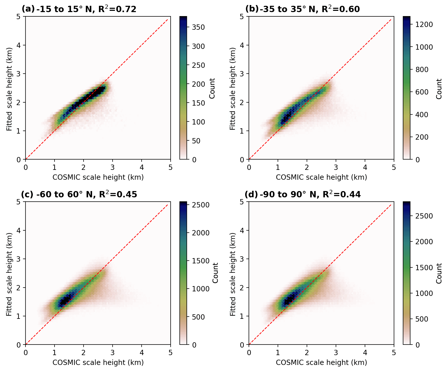
Figure 9 2D histograms of the distribution between the parameterized scale height and the COSMIC scale height over ocean for selected global latitude zones.

Altogether, we have to fit 35 parameters to the complete data set of calculated COSMIC scale heights for the parameterization of the scale height over ocean. The goodness of the parameterization in approximating the scale height is illustrated in Fig.9 for different latitude zones. For the latitude zones including the tropics (−15 to 15^∘ N) and subtropics (−35 to 35^∘ N) we find a good agreement between the parameterization and the calculated COSMIC scale height, with R² of 0.72 and 0.60 respectively. However, including higher latitudes in the evaluation, i.e. midlatitudes (−60 to 60^∘ N) and polar regions (−90 to 90^∘ N), leads to an increased scatter and a worsening of the parameterization (R² of 0.45 and 0.44 respectively). This inferior agreement is likely caused by the larger atmospheric variability in the midlatitudes (e.g. higher atmospheric dynamics) as well as an increased uncertainty in the COSMIC water vapour profile measurements due to lower water vapour concentrations.

3.3.2 Land

Figure 7 already revealed much larger scatter in the distribution of COSMIC TCWV and COSMIC scale height for data over land, indicating that the water vapour profile shape over land surface is less homogeneous than over ocean, likely due to further heterogeneously distributed water vapour sources, such as evapotranspiration by plants and soil. Thus, the H₂O VCD and scale height are likely to be dependent on the amount of vegetation; i.e. high vegetation is associated with high evapotranspiration and high water vapour concentrations near the ground, and thus the scale height should be close to the scale height over ocean. In contrast, low amounts of vegetation are associated with less evapotranspiration and a usually drier atmosphere, indicating that the scale height should be higher than over ocean.

To quantify the amount of vegetation, we use the Normalized Difference Vegetation Index (NDVI), where a value of 1.0 indicates high vegetation and a value around 0.0 indicates low vegetation. As data source for the NDVI, we use data within the MODIS Aqua MYDC13C2 Version 6 product (Didan et al., 2015) and continue as follows: first, we calculate the parameterized scale height H_ocean assuming an ocean surface globally. Then we calculate the ratio of the calculated COSMIC scale height over land H_land and the parameterized scale height H_ocean.

Figure 10 2D histograms of the distribution between the ratio H_land∕H_ocean against the NDVI for different filtered data sets: panel (a) includes all data points, panel (b) includes all points except those with MODIS landcover type 15 (corresponding to deserts), and panel (c) includes all points except landcover types 7 (corresponding to open shrublands) and 15. The red solid line represents the fit result using the Siegel algorithm with details of the fit results in the legends of each panel.

Figure 10 shows the ratio H_land∕H_ocean as a function of the NDVI for data sets filtered by different landcover types and the solid red lines represent the robust regression results (summarized in Table 3) using the model from Siegel (1982). Panel (a) depicts the distribution for which no filter is applied. Except for low NDVI values, a linear relation between the ratio and NDVI is observable; however, for NDVI values around 0.1 the ratio varies strongly, between 0.7 and 3.0. In the centre panel we use the landcover classification from the MODIS Aqua MCD12C1 Version 6 product (Sulla-Menashe et al., 2019) to filter measurements for locations classified as landcover type 15 (corresponding to a desert). With this filter the ratio now only varies between 0.7 and 1.5, with a weak dependence on the NDVI. If we further filter locations of landcover type 7 (corresponding to open shrublands), the fit results of the robust regression change only slightly compared to the first filtered data set.

Table 3 Fit results of the robust regression between the ratio of scale heights H_land∕H_sum and the NDVI for different filtered data sets.

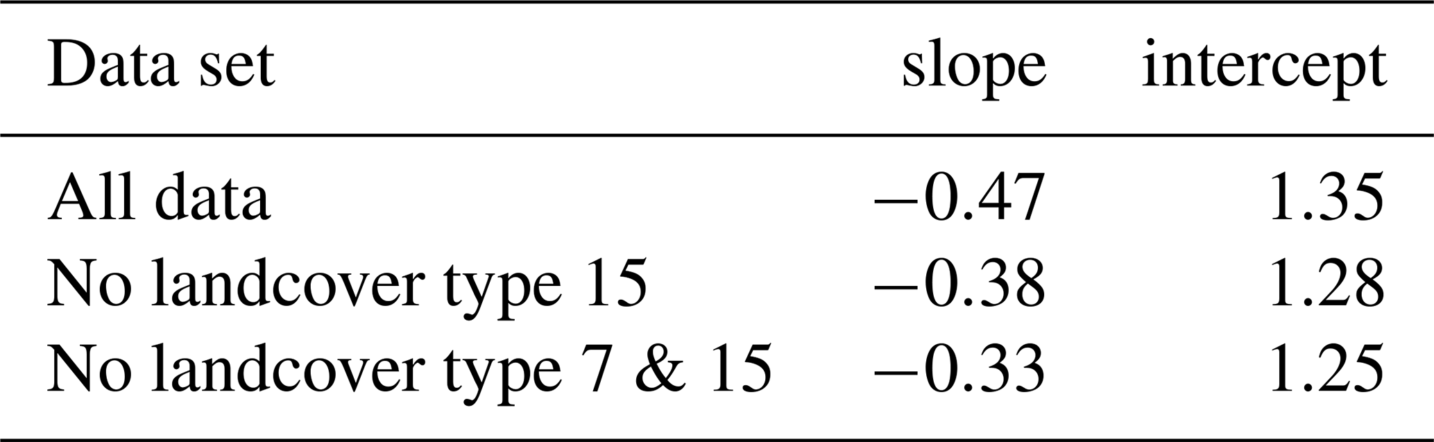
Hence the scale height over land H_land can be approximated as the scale height over ocean H_ocean multiplied by a first-order polynomial of the NDVI:

$$\begin{array}{}\text{(13)}& H_{\mathrm{land}}=H_{\mathrm{ocean}}(\mathrm{VCD},\mathit{\theta },t)\cdot \left({\mathit{\gamma }}_{\mathrm{land}}+{\mathit{\delta }}_{\mathrm{land}}\cdot \mathrm{NDVI}\right),\end{array}$$

whereby in the following we use the results for the data set filtered for landcover types 7 and 15 globally. Since regions of landcover types 7 or 15 are usually arid, the retrieved H₂O VCD is small, and thus the error due to an inadequate parameterization of the AMF is much smaller than the fit error of the spectral analysis.

3.4 Iterative retrieval scheme

For the calculation of the H₂O VCD we precomputed AMF look-up tables (LUTs) for the different water vapour profile shapes with scale heights ranging from 0.5 to 5.0 km. These LUTs can then be used within a fixed-point iteration. In our case the iterative retrieval scheme is based on a fixed-point iteration according to Steffensen's method (Steffensen, 1933; Wendland and Steinbach, 2005):

$$\begin{array}{}\text{(14)}& \begin{array}{rl}{\mathrm{VCD}}_{i+\mathrm{1}}& ={\mathrm{VCD}}_i\\ & -{\displaystyle \frac{{\left[f\left({\mathrm{VCD}}_i\right)-{\mathrm{VCD}}_i\right]}^{\mathrm{2}}}{f\left(f\left({\mathrm{VCD}}_i\right)\right)-\mathrm{2}\cdot f\left({\mathrm{VCD}}_i\right)+{\mathrm{VCD}}_i}},\end{array}\end{array}$$

where f is a function calculating the scale height for a given VCD using Eqs. (10) and (13), applying it to the precomputed AMF look-up tables and from that returning a new VCD. The advantage of Steffensen's method is that it does not need a derivative and is able to determine the fixed point even for the case of a non-contractive function (Wendland and Steinbach, 2005). For the first guess we derived the initial VCD from the SCD using a geometric AMF $\left({\mathrm{AMF}}_{\mathrm{geo}}=\frac{\mathrm{1}}{\cos \left(\mathrm{SZA}\right)}+\frac{\mathrm{1}}{\cos \left(\mathrm{VZA}\right)}\right)$ and stop the iteration as soon as the logarithmic difference between two consecutive results is smaller than 5 % (approximately 1 kg m⁻² assuming an average H₂O VCD of 20 kg m⁻²) or after six iteration steps. We also checked other values for the first guess and could confirm that the convergence of the iterative scheme is independent of them.

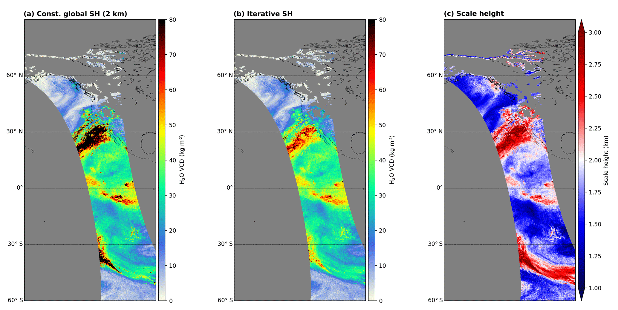
Figure 11 Comparison of the H₂O VCD calculated using a global constant a priori profile shape of 2 km (a) and the iterative scale height method (b) for all-sky conditions. Panel (c) illustrates the water vapour scale height estimated within the retrieval's VCD conversion. All panels show an atmospheric river hitting the eastern Pacific/western US coast on 13 February 2019. Invalid pixels are coloured grey.

Figure 11 illustrates a comparison of H₂O VCD distributions for the cases of using a global constant a priori water vapour profile shape (panel a) with a scale height of 2 km (in accordance with Weaver and Ramanathan, 1995) and using the iterative scale height approach (centre panel) for all-sky conditions (i.e. no cloud filter applied) during an atmospheric river event at the western coast of the US on 13 February 2019. Figure 11c depicts the distribution of the water vapour scale height yielded during the iterative VCD conversion. The water vapour scale height varies a lot along the orbit and differs distinctively from 2 km, causing large deviations between the two approaches, particularly at pixels with high TCWV values and for clouded pixels. However, in contrast to the approach with a constant scale height, the iterative approach is still able to give reasonable TCWV results and does not exceed values higher than 80 kg m⁻².

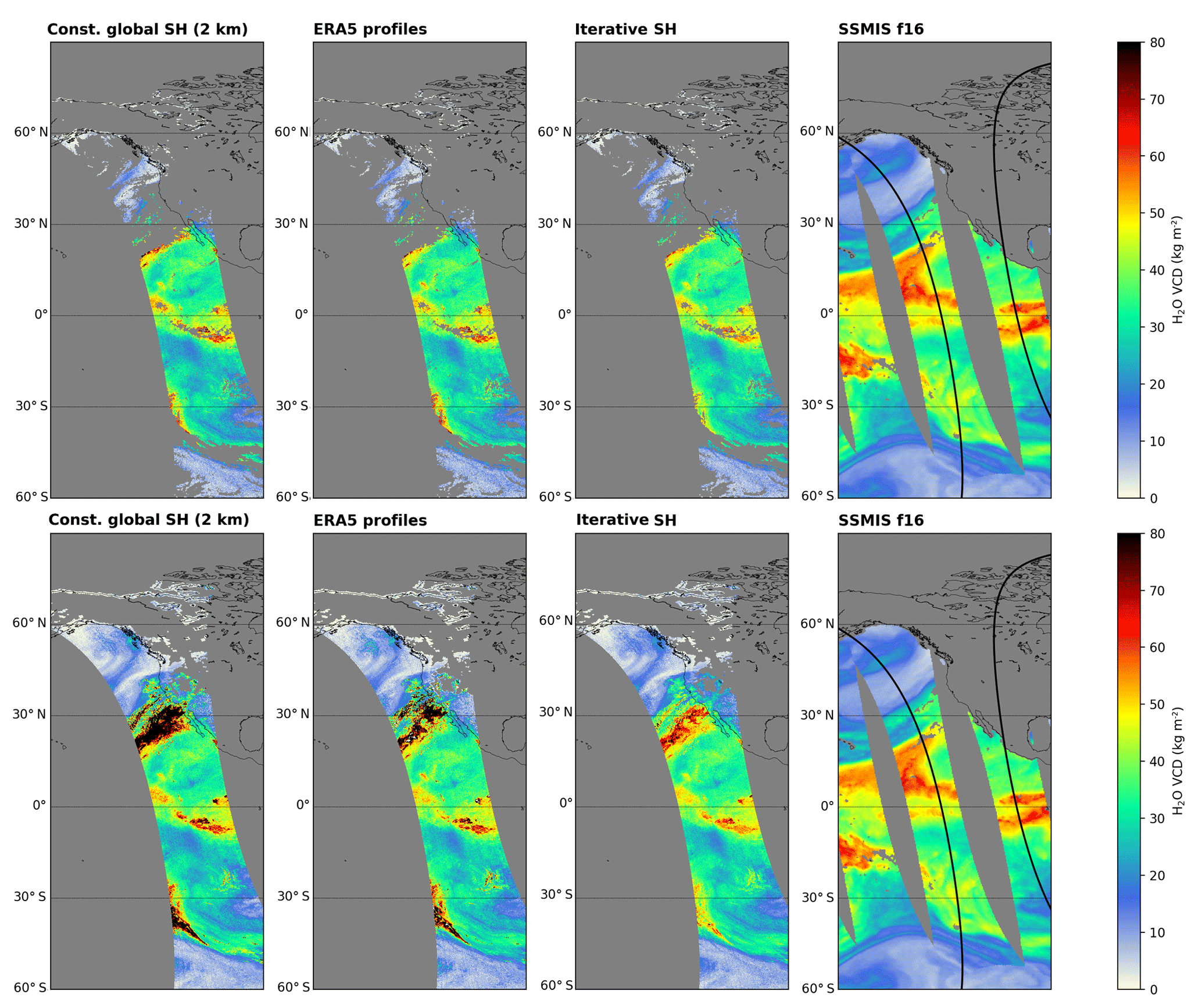
Figure 12 Comparison of the H₂O VCD calculated using a global constant a priori profile shape of 2 km (first from left), ERA-5 profiles (second from left), and the iterative scale height method (third from left) for clear-sky (effective cloud fraction <20 %; top row) and cloudy-sky conditions (effective cloud fraction ≤100 %; bottom row) with TCWV from SSMIS f16 (right) for the same scenery as in Fig. 11. Invalid pixels are coloured grey. The solid black lines indicate the edges of the TROPOMI swath.

Figure 12 illustrates the H₂O VCD distributions from calculations using constant, ERA-5, and iterative profile shapes for the same scenario for clear-sky (effective cloud fraction CF<20 %, top row) and all-sky (CF≤100 %, bottom row) conditions. For ERA-5 we used the data provided by Copernicus Climate Change Service (2018a) on an hourly $\mathrm{0.25}{}^{\circ }\times \mathrm{0.25}{}^{\circ }$ grid and interpolated the model profile data to the TROPOMI pixel centre coordinates. In addition to the TROPOMI H₂O VCDs, Fig. 12 also depicts the TCWV distribution from microwave sensor SSMIS f16, which has a temporal difference of around +2.3 h.

For the clear-sky case (top row) the VCD distributions between all profile approaches are almost identical, whereby for the constant scale height approach (first panel from the left) very high VCDs (exceeding values higher than 80 kg m⁻²) can be observed at the edges of the cloudy regions in the northern subtropics. For the all-sky case (bottom row) the differences between all approaches are largest in cloudy regions: for instance, in the region of the atmospheric river, the VCDs from the constant and ERA-5 profiles distinctively overestimate the VCD and exceed values higher than 80 kg m⁻². In contrast, even under these unfavourable observation conditions the iterative approach is still able to give reasonable VCD values. Furthermore, the iterative approach shows an overall good agreement with the SSMIS observations.

Figure 13 Mean normalized Box-VCD profiles of ERA-5 and the iterative scale height approach for cases of distinctive VCD disagreement within the region of the atmospheric river. Panel (a) illustrates the mean of the selected profiles from the ground up to 15 km and panel (b) the mean of the same profiles, but from the cloud top up to 6 km above the cloud top. The solid lines indicate the mean profiles and the shaded areas the corresponding 1σ standard deviation.

Taking a closer a look at the reasons for the deviations of the results retrieved for the ERA-5 profiles, Fig. 13 depicts the mean of the normalized water vapour profiles of ERA-5 and the iterative scale height approach for the AR region (around 30^∘ N). Figure 13a shows the water vapour profile from the ground up to 15 km. In comparison to the iterative approach, ERA-5 is much drier above approximately 2.5 km for these particular cases, indicating that ERA-5 might systematically underestimate the water vapour content above the cloud within the region of the atmospheric river. This finding is further supported by Fig. 13b, which illustrates the normalized water vapour profiles above the cloud top: ERA-5 profiles are close to 0 and show only small variations, whereas the profiles of the iterative approach indicate higher water vapour concentrations along with a much higher variability. One potential reason for the discrepancies of ERA-5 could be the missing observational input data for the reanalysis: without observations, the reanalysis model is dominated by its a priori information (e.g. a climatological mean), so that it can be systematically distorted from the real atmosphere. However, further investigations of possible ERA-5 biases are beyond the scope of this paper.

4 Evaluation of different surface albedo input data

The surface albedo has a strong impact on the radiative transfer and thus also on the AMF. Hence we investigated the impact of different albedo products on the TCWV retrieval: the OMI monthly (a) mean and (b) minimum Lambertian equivalent reflectance (LER) at 442 nm from Kleipool et al. (2008) and (c) MODIS Aqua blue surface reflectance from the MODIS MYD13C2 Version 6 product (Didan et al., 2015). The MODIS reflectance covers a broad spectral window from 459 to 479 nm. Thus, to account for the different spectral windows of the albedo products, we scale the MODIS albedo by factor of 0.9. This factor was estimated by calculating the ratio between 472 and 442 nm of the OMI yearly minimum LER over parts of Australia where cloud contamination is generally low and hence the OMI LER has reasonably accurate values.

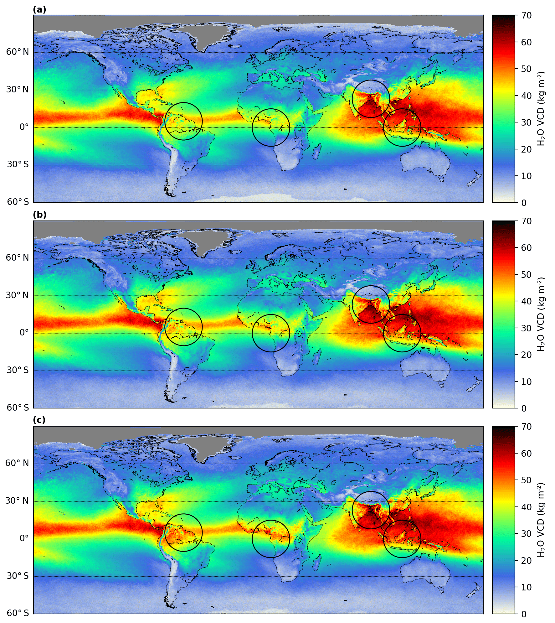
Figure 14 Comparison of the effect of different land albedo input data on the mean H₂O VCD for boreal summer 2018 (a: OMI monthly mean LER, b: OMI monthly minimum LER, c: scaled MODIS Aqua blue surface reflectance). Only pixels with an effective cloud fraction smaller than 20 % are included.

Figure 14 illustrates the global mean H₂O VCD of boreal summer 2018 for the different albedo input data over land (top row: monthly mean OMI LER, middle row: monthly minimum OMI LER, bottom row: scaled monthly MODIS Aqua blue surface reflectance). In the tropical and subtropical regions the OMI albedos cause a distinctive separation of the VCDs between land and ocean, in particular at the coasts of South America, Africa, and Indonesia. These aforementioned regions are often affected by cloud cover, which might cause the OMI albedo statistics to be unable to filter cloudy cases correctly, so that cloud-contaminated observations are used within the albedo calculations. As a consequence, the values in the OMI albedo are too high and lead to an overestimation of the AMF, which in turn causes an underestimation of the H₂O VCD.

In contrast, MODIS pixels have a much higher spatial resolution and MODIS' NIR channels are more sensitive to cloud contamination, yielding a higher sample size and allowing for correct cloud filtering. Hence, the H₂O VCD distribution using the MODIS surface reflectance results in a much smoother transition from ocean to land and in general much higher VCD values over land along the Equator. Thus, in the following we use a combination of the MODIS and OMI albedos: the scaled MODIS Aqua blue surface reflectance over land and the monthly minimum OMI albedo over ocean.

5 Uncertainty estimation

The error budget of the H₂O VCD is determined by the propagation of the main error sources of the fitted SCD and the precalculated AMF. Errors in the SCD are mainly caused by random errors, like the photon noise, and systematic errors, e.g. the uncertainty of the absorption cross section, whereas errors in the AMF are mostly systematic with random contributions.

5.1 Uncertainties in the slant column density

Table 4 summarizes the different error sources for the H₂O SCD and the corresponding estimated uncertainties. As demonstrated in Sect. 2.1 and Appendix B the water vapour absorption cross section varies systematically between the different HITRAN versions. Hence, we assumed that the uncertainty of the water vapour cross section is of the same order of magnitude as the changes between the different cross-section versions, i.e. approximately around 10 %. Considering the LP-DOAS comparisons (see Sect. 2.1 and Appendix B) we estimate these errors to be around 5 % for this study.

Table 4 Summary of the different error sources considered in the H₂O SCD uncertainty.

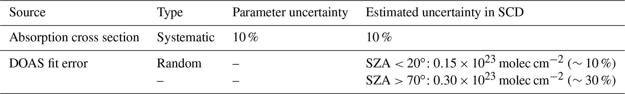
Figure 15 Histograms of the standard H₂O SCD fit error distribution for small (SZA<20^∘, a, c) and large ($\mathrm{70}{}^{\circ }<\mathrm{SZA}\le \mathrm{90}{}^{\circ }$, b, d) solar zenith angles for relatively small (<3 %, orange) and high (>15 %, blue) surface albedo values for clear-sky (cloud fraction <5 %, a, b) and cloudy-sky (cloud fraction >20 %, c, d) conditions. The coloured dashed lines represent the median of the respective distributions and their values are given in the legend of each panel.

The retrieval's spectral analysis directly yields the 1σ standard fit error of the H₂O SCD, which is usually dominated by noise. For a better understanding of these fit errors, we separated them into data for small/large solar zenith angles (SZA<20^∘ and $\mathrm{70}{}^{\circ }<\mathrm{SZA}\le \mathrm{90}$^∘ respectively), low/high surface albedo (<3 % and >15 % respectively), and clear-/cloudy-sky observation conditions (CF<5 % and CF>20 % respectively). The distributions of the standard and relative fit errors of the spectral analysis are given in Figs. 15 and 16 respectively. The median values in Fig. 15 indicate that the standard errors for high SZA (around 0.3×10²³ molec cm⁻²) are twice as high as for small SZA (around 0.15×10²³ molec cm⁻²). Under clear-sky conditions the standard error for small surface albedo values is larger than for high surface albedo, but for cloudy conditions it does not depend on the surface albedo.

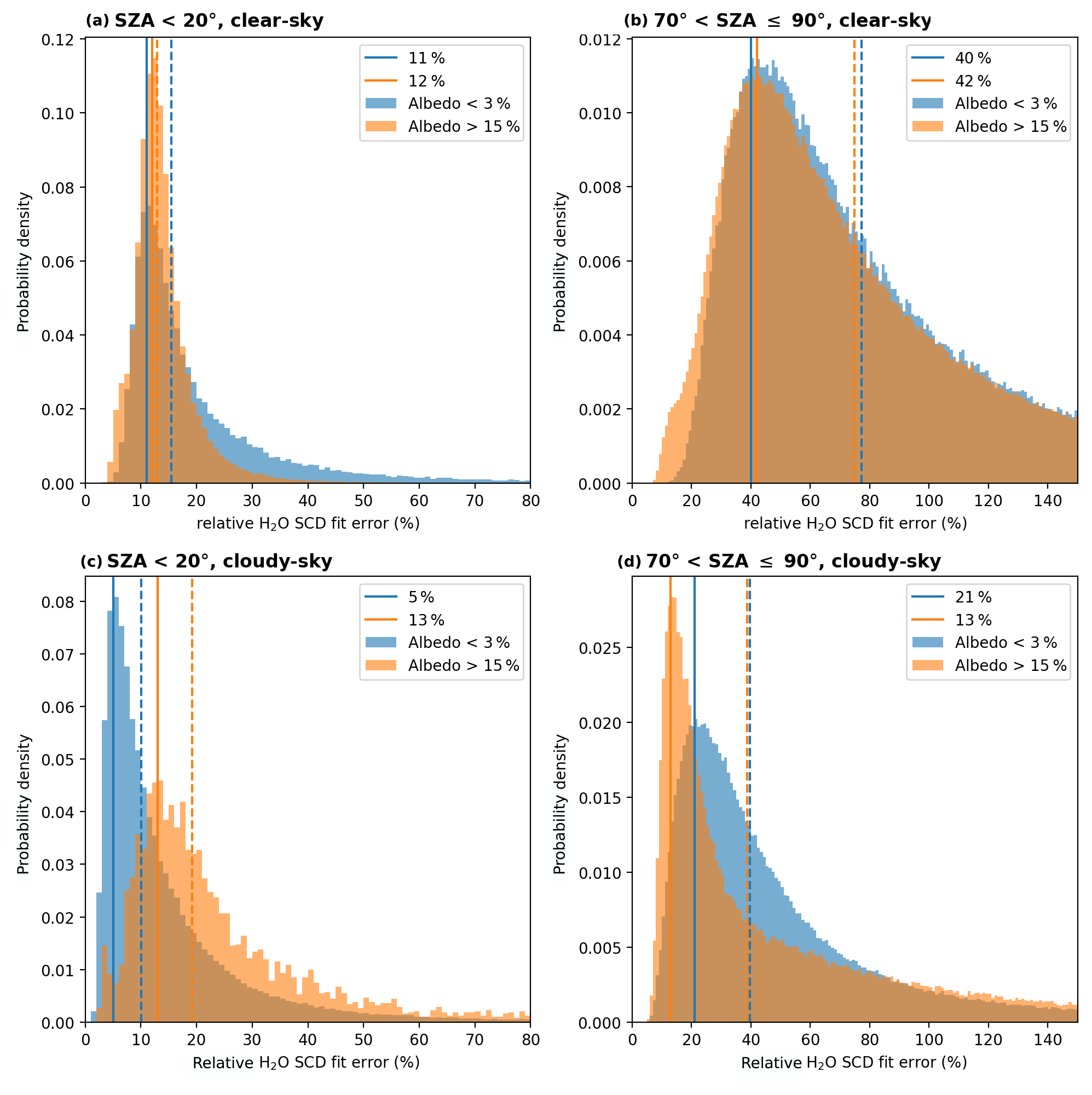
Figure 16 Histograms of the relative H₂O SCD fit error distribution for small (SZA<20^∘, a, c) and large ($\mathrm{70}{}^{\circ }<\mathrm{SZA}\le \mathrm{90}{}^{\circ }$, b, d) solar zenith angles for relatively small (<3 %, orange) and high (>15 %, blue) surface albedo values for clear-sky (cloud fraction <5 %, a, b) and cloudy-sky (cloud fraction >20 %, c, d) conditions. The coloured dashed lines represent the median of the respective distributions and the solid lines represent the location of maximal probability density (values given in the legend of each panel).

Figure 16 reveals that the relative fit errors for high SZAs are higher than for low SZAs. However, the locations of maximal probability density and the medians also indicate that the distributions are right-skewed, in particular for high SZA scenarios: for these scenarios the relative errors easily exceed values of 100 %. Nevertheless, using the locations of maximal probability density as a rule-of-thumb estimate, relative fit errors have values around 10 % for low SZAs and approximately 30 % for high SZAs.

To estimate errors associated with ISRF biases, we calculated the H₂O SCD using a Gaussian ISRF (instead of an asymmetric Super-Gaussian) for orbit 6930 and compared them to the SCDs from the “standard” retrieval setup for SZA<88^∘. The comparison depicted in Fig. S3 reveals that the SCDs using the Gaussian ISRF highly correlate with the “standard” SCDs and only differ by approximately 1 %. Considering the much higher fit errors, errors due to biases in the ISRF are negligible.

5.2 Uncertainties in the AMF

The uncertainty in the AMF depends on the uncertainty of its input parameters. Because the parameters of the viewing geometry (i.e. solar zenith angle, line-of-sight angle, and solar relative azimuth angle) are known with high accuracy, the most important uncertainties are uncertainties of the surface albedo, cloud fraction, cloud top height, and water vapour profile shape. In order to estimate the contribution of each input parameter to the overall AMF uncertainty, we define standard scenarios (summarized in Table 5) for which we calculate the AMF from the precalculated LUT. Then we vary the input parameter for each scenario according to its uncertainty assumption listed in Table 6. The uncertainties of the water vapour scale height have been derived from the fit results of the intercomparisons between the measured COSMIC scale height and the parameterized scale height over ocean (see Fig. 9) and land (see Fig. 10).

Table 5 Standard retrieval scenarios for the estimation of AMF error.

Kleipool et al. (2008)Veefkind et al. (2016)

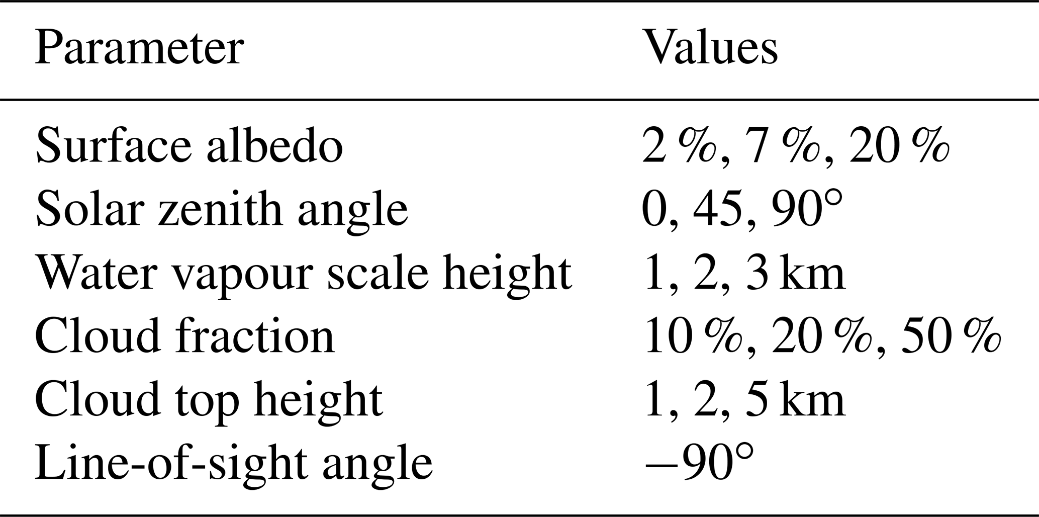
Table 6 Summary of different error sources considered in the AMF uncertainty.

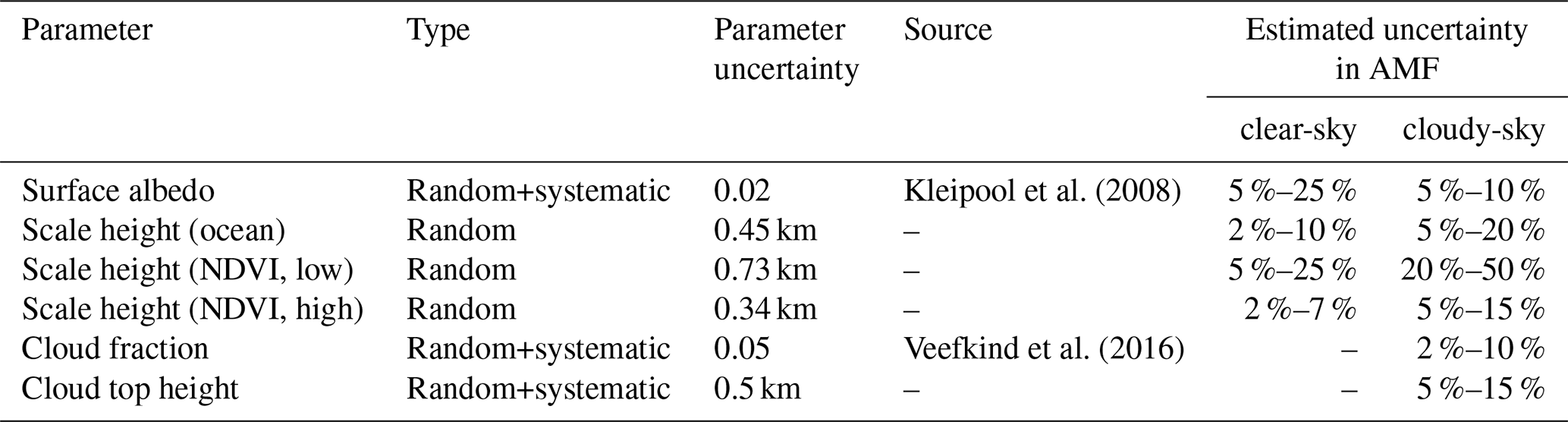
Figure 17 depicts box–whisker plots of the relative AMF error due to uncertainties in surface albedo and scale height for the standard clear-sky scenarios of surface albedo, solar zenith angle, and scale height. It reveals that uncertainties in surface albedo and scale height over low vegetation have the strongest impact on the AMF and can cause AMF errors larger than 30 %, in particular for scenarios with low surface albedo or high solar zenith angle. On average the median values of the AMF errors typically vary around approximately 10 %.

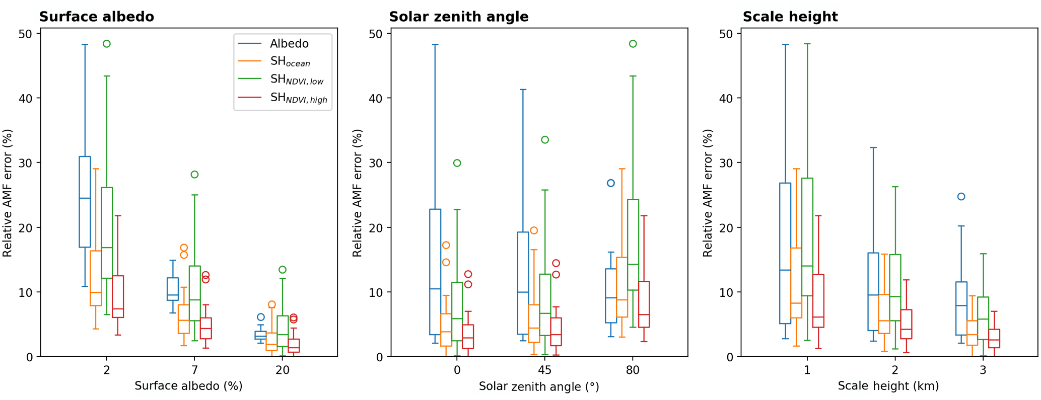
Figure 17 Box–whisker plots of the relative AMF errors for clear-sky conditions due to uncertainties within the retrieval's input parameters (blue: surface albedo, orange: scale height over high vegetation, green: scale height over low vegetation, red: scale height over ocean) according to the uncertainty assumptions in Table 6 and simulated for the standard scenarios of the surface albedo, solar zenith angle, and scale height given in Table 5.

Figure 18 Box–whisker plots of the relative AMF errors for cloudy-sky conditions due to uncertainties within the retrieval's input parameters according to the uncertainty assumptions in Table 6 and simulated for the standard scenarios given in Table 5.

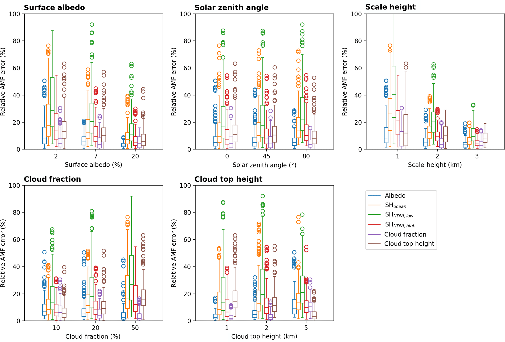
Figure 18 illustrates box–whisker plots of the relative AMF error due to uncertainties in surface albedo, scale height, cloud fraction, and cloud top height for all standard scenarios listed in Table 5. In contrast to the clear-sky scenarios, the impact of the surface albedo uncertainties has strongly decreased, but in general the contributions of all AMF errors have increased distinctively. The main source of the AMF errors is still the uncertainty of the scale height over low vegetation, whose median values vary between 20 % and 50 % but can also cause AMF errors larger than 60 %.

Table 6 summarizes the results of the different error sources considered in the AMF uncertainty for clear- and cloudy-sky conditions. For clear-sky conditions one can typically assume a relative AMF error around 10 %–15 % and for cloudy-sky conditions around 10 %–25 %.

5.3 Total H₂O VCD uncertainty

The total relative H₂O VCD uncertainty can be approximated by

$$\begin{array}{}\text{(15)}& {\displaystyle \frac{\mathrm{\Delta }\mathrm{VCD}}{\mathrm{VCD}}}=\sqrt{{\left({\displaystyle \frac{\mathrm{\Delta }\mathrm{AMF}}{\mathrm{AMF}}}\right)}^{\mathrm{2}}+{\left({\displaystyle \frac{\mathrm{\Delta }\mathrm{SCD}}{\mathrm{SCD}}}\right)}^{\mathrm{2}}}.\end{array}$$

With our findings of typical relative AMF and H₂O SCD uncertainties, the total relative VCD uncertainty is typically around 10 %–20 % for observations during clear-sky conditions, over ocean surface, and at low solar zenith angles. During partly cloudy-sky conditions, over land surface, and at high solar zenith angles the error reaches values of approximately 20 %–50 %.

6 Validation study

In order to evaluate the retrieval's performance, we conducted a validation study for the time ranges of boreal summer (June, July, and August) 2018 and boreal winter (December, January, and February) 2018/2019 whereby we only include clear-sky observations (i.e. pixels with an effective cloud fraction smaller than 20 %) and ice- and snow-free pixels. To avoid extreme outliers, we only include observations with an AMF>0.1. As reference data for the validation we use TCWV from the Special Sensor Microwave Imager/Sounder (SSMIS), from the reanalysis model ERA-5, and the ground-based GPS network SuomiNet. For the sake of completeness, we also briefly investigate higher cloud fractions at the end of each subsection and provide the results in the Supplement.

As cloud input data we use the cloud information (effective cloud fraction at 440 nm and cloud top height) as well as the surface altitude from the TROPOMI L2 NO₂ product (Van Geffen et al., 2019) and as surface albedo input data we use the combination of the modified MODIS and OMI albedo described in Sect. 4. To distinguish between ocean and land surface, we use a land–sea mask derived from GSHHS coastline data (Wessel and Smith, 1996), in which we use the pixel centre coordinates for the separation into land and ocean. As the NDVI is not available over lakes, we treat them as ocean.

6.1 SSMIS comparison

For the evaluation we use measurements from SSMIS onboard NOAA's f16 and f17 satellites processed by Remote Sensing Systems (RSS) and provided by the NASA Global Hydrology Resource Center on a daily $\mathrm{0.25}{}^{\circ }\times \mathrm{0.25}{}^{\circ }$ grid. SSMIS can observe the TCWV distribution under all-sky conditions over ocean with an accuracy of around 1 kg m⁻² (Wentz, 1997; Mears et al., 2015). Since SSMIS changes its Equator crossing time (ECT), we only include SSMIS observations whose ECT is within 3 h (and 5 h for f17 respectively) with respect to TROPOMI's ECT of 13:30 LT. For the intercomparison we only include SSMIS measurements that are not affected by rain.

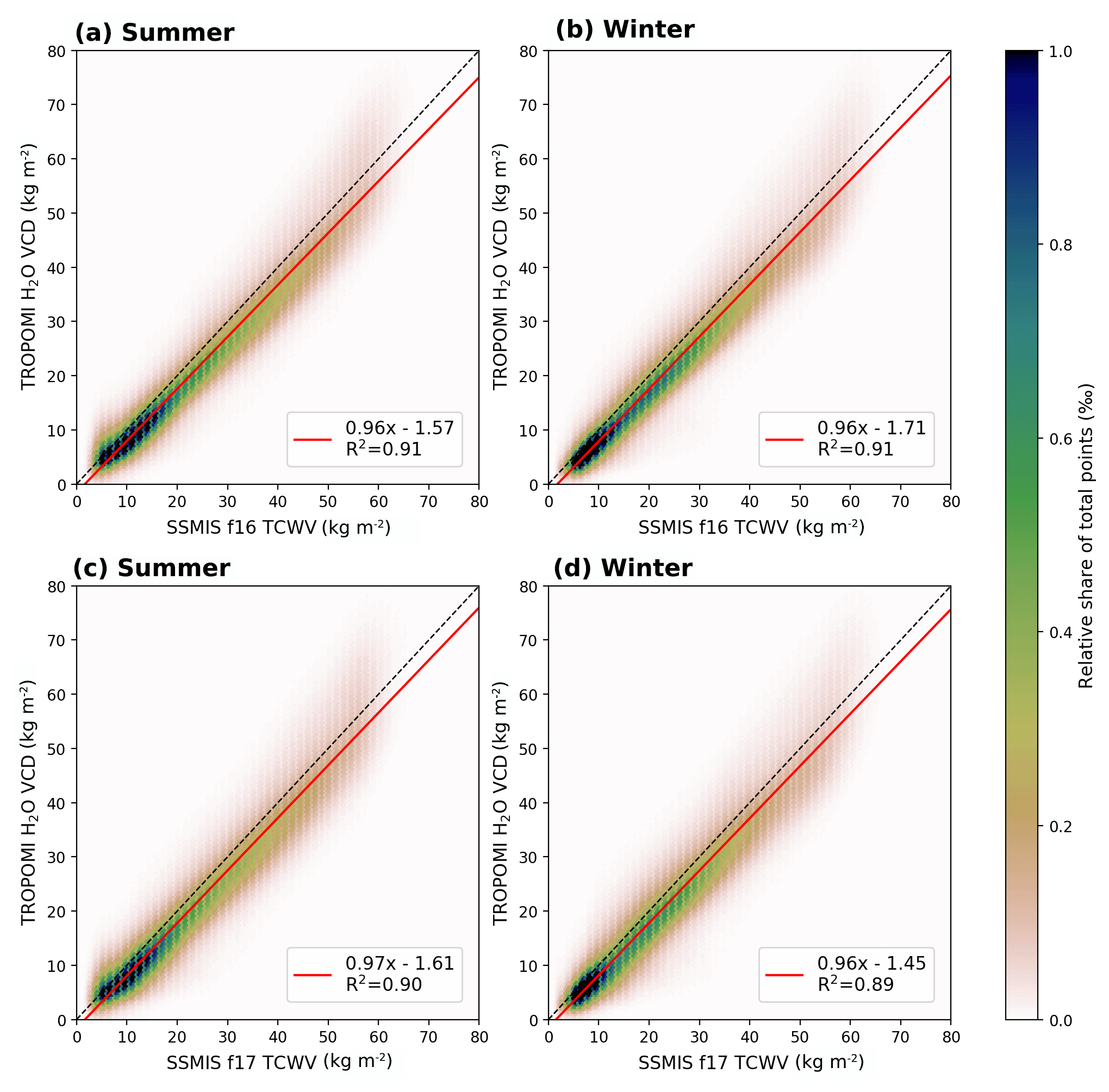
Figure 19 2D histograms for the comparison between TROPOMI and SSMIS f16 (a, b) and f17 (c, d) for clear-sky conditions (CF<20 %) for boreal summer (a, c) and boreal winter (b, d), where the colour indicates the relative share of total data points. The black dotted line indicates the 1-to-1 diagonal and the red solid line represents the results of the linear regression. The parameters of the linear regression and the coefficient of determination are given in the box in each panel.

Figure 19 depicts the comparison between SSMIS (f16, top row, and f17, bottom row) and TROPOMI for boreal summer (left column) and winter (right column). For f16 (top row) the scatter is distributed closely along the 1-to-1 diagonal (dashed lines) for both seasons and the fitted regression lines (red solid lines) indicate a very good agreement between both data, with slopes around 0.96, intercepts around −1.6 kg m⁻² for summer and −1.7 kg m⁻² for winter, and coefficients of determination of R²=0.91. For f17 the comparison reveals similar agreement, with slopes around 0.97 and intercepts around −1.5 kg m⁻² with R²=0.89 for both seasons. Overall, considering the differences in collocation time (3 and 5 h for f16 and f17 respectively), the comparison shows that the TROPOMI TCWV retrieval can well capture the water vapour distribution over ocean.

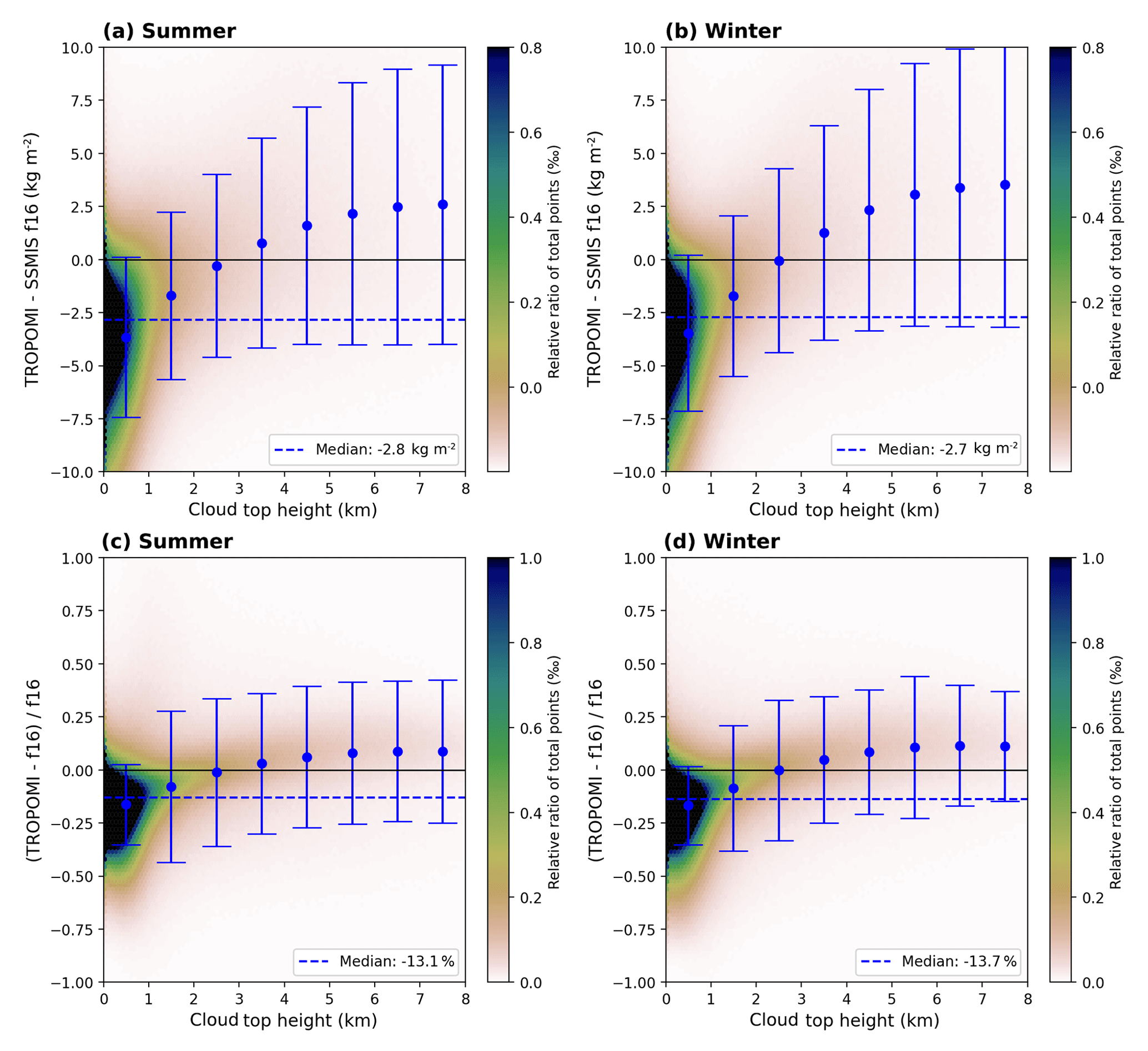
Figure 20 2D histograms of the difference (TROPOMI − SSMIS f16, a, b) and relative difference $(\mathrm{TROPOMI}-\mathrm{f}\mathrm{16})/\mathrm{f}\mathrm{16}$ (c, d) as a function of the input cloud top height (CTH) for clear-sky conditions (CF<20 %) for summer (a, c) and winter (b, d). The blue dashed line represents the median over the whole CTH range. The blue dots represent the median within a 1 km CTH and the error bars represent their respective 1σ standard deviation.

Figure 21 Same as Fig. 20 but for SSMIS f17.

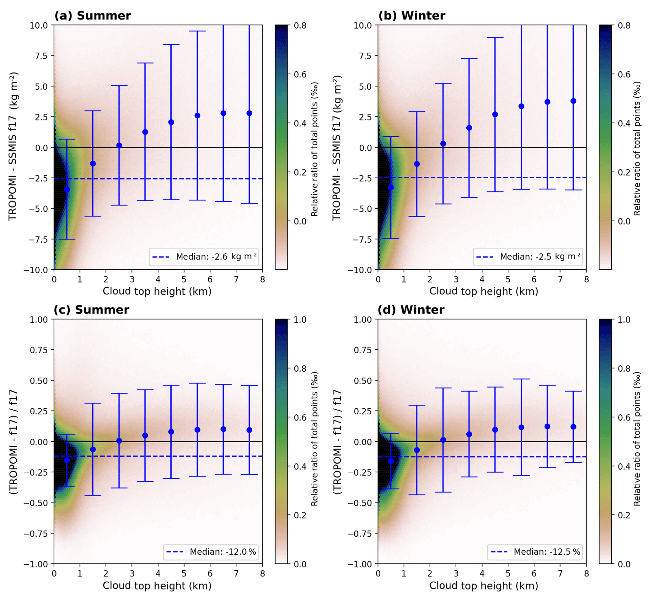
To investigate the influence of clouds on our retrieval, we plot the difference (top row) and relative difference (bottom row) between TROPOMI and SSMIS as a function of the input cloud top height (CTH) in Figs. 20 and 21 for f16 and f17 respectively. The median over the whole CTH range (blue dashed line) indicates an underestimation of the TROPOMI H₂O VCD of approximately 12 %–13 % (2.6 kg m⁻²). However, the large majority of data points is distributed within the CTH bin between 0 and 1 km, revealing that the underestimation of the TROPOMI TCWV is mainly caused by low clouds. For mid-level clouds the median difference almost cancels out, whereas for high clouds it first increases and then remains almost constant with cloud top height.

Further validation results for SSMIS f16 and f17 separated into different cloud fraction and cloud top height bins for July 2018 are given in Figs. S10 and S11 respectively. The results indicate that there is no dependency with cloud fraction but a distinctive dependency with cloud top height: the retrieval underestimates for clouds below 1 km, is in very good agreement for mid-level clouds (1–4 km), and overestimates for higher clouds.

6.2 ERA-5 comparison

For the intercomparison between the reanalysis model ERA-5 and TROPOMI, we use ERA-5 TCWV data provided by Copernicus Climate Change Service (2018b) on a $\mathrm{0.25}{}^{\circ }\times \mathrm{0.25}{}^{\circ }$ grid. We only take into account values which are within +1 h with respect to the starting sensing time of the TROPOMI orbit and separate the data into data over ocean and data over land.

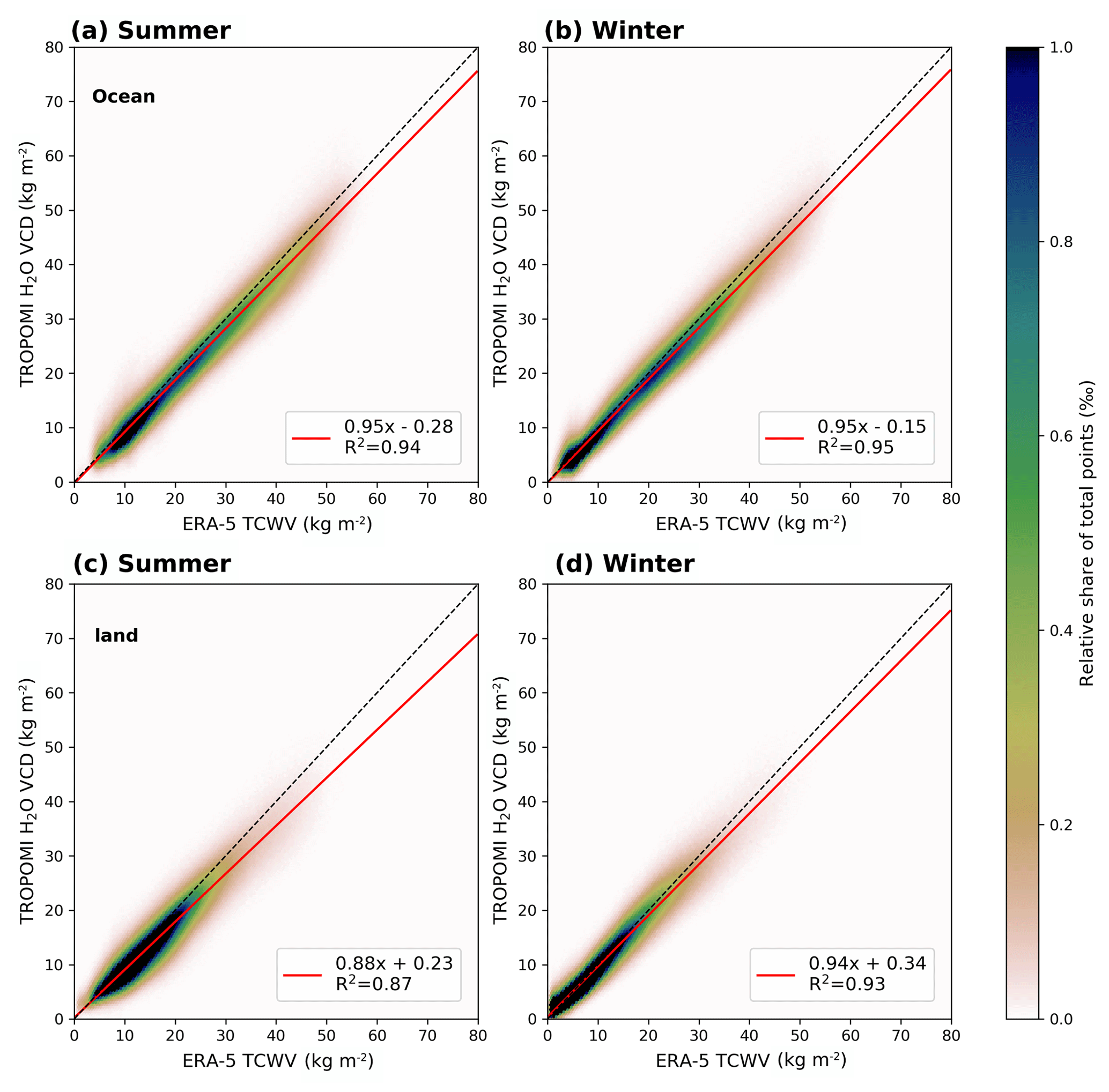
Figure 22 2D histograms for the comparison between TROPOMI and ERA-5 for data over ocean (a, b) and over land (c, d) for clear-sky conditions (CF<20 %) for boreal summer (a, c) and boreal winter (b, d), where the colour indicates the relative share of total data points. The black dotted line indicates the 1-to-1 diagonal and the red solid line represents the results of the linear regression. The parameters of the linear regression and the coefficient of determination are given in the box in each panel.

The results of the intercomparison are summarized in Fig. 22. Over ocean (top row in Fig. 22) the results are similar to the results from the comparison between TROPOMI and SSMIS: apart from slopes close to 0.95 and intercepts close to zero, the linear regression yields R² of 94 % for summer and 95 % for winter respectively. Over land the linear regression still yields high values of the coefficient of determination R², but the TROPOMI retrieval generally underestimates the H₂O VCD by approximately 12 % during summer (and 7 % during winter). Since the values of the correlation coefficient are still high and the values over ocean coincide very well with the reference data sets, we assume that this underestimation has to be caused by a systematic uncertainty within the input parameters for our retrieval.

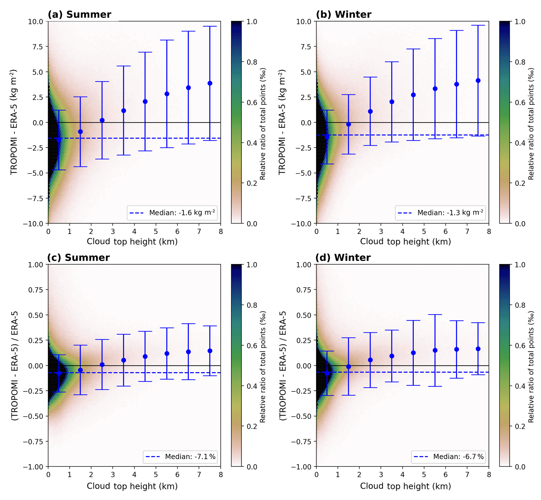
Figure 23 2D histograms of the difference (TROPOMI − ERA-5, a, b) and relative difference $(\mathrm{TROPOMI}-\text{ERA-5})/\text{ERA-5}$ (c, d) as a function of the input cloud top height (CTH) for clear-sky conditions (CF<20 %) for summer (a, c) and winter (b, d) for data over ocean. The blue dashed line represents the median over the whole CTH range. The blue dots represent the median within a 1 km CTH and the error bars represent their respective 1σ standard deviation.

The influence of the cloud top height input is illustrated in Fig. 23 for data over ocean. The median is around −1.6 kg m⁻² (−7.1 %) and −1.3 kg m⁻² (−6.7 %) during summer and winter respectively, whereby similarly to SSMIS, these underestimations are caused by the majority of data points within the 0–1 km CTH bin. For increasing CTH the deviation from the reference increases and leads to an overestimation. For data over land (Fig. 24) the CTH variability is much larger than over ocean; i.e. most data points are now distributed between 0 and 3 km and the median is around values of −1.5 kg m⁻² (−10.3 %) and −0.4 kg m⁻² (−4.0 %) during summer and winter respectively. Furthermore, low clouds still cause an underestimation, and for mid- to high-level clouds the deviations almost cancel out, but one can also observe an increasing scatter for winter data.

Figure 24 Same as Fig. 23 but for data over land.

All these findings reveal that the combination of albedo uncertainties and uncertainties in the cloud properties (cloud fraction and cloud top height) as well as in the scale height parameterization have a distinctive influence on the AMF. The cloud products from TROPOMI rely on the OMI albedo which, as we have demonstrated in Sect. 4, has several problems over land surface. In addition, the uncertainty of the OMI albedo over land surface is higher than over ocean due to a highly spatiotemporal variability of the scenery, and the differences between the monthly minimum and the monthly mean albedo are higher over land than over ocean. Furthermore, the cloud top height is calculated via the cloud top pressure and has to be combined with the surface pressure. Thus, the uncertainty of the cloud top height over land is higher than over ocean, since over ocean the topography is much simpler.

Nevertheless, the complex radiative interactions between albedo and clouds might amplify or cancel out these deviations and thus make it difficult to draw clear conclusions.

As for the SSMIS comparison, further validation results for ERA-5 over ocean and land separated into different cloud fraction and cloud top height bins for July 2018 are given in Figs. S12 and S13.

Similarly to SSMIS, the results over ocean reveal an underestimation for low clouds and an overestimation for high clouds and that there is almost no dependency with cloud fraction. Over land low clouds still cause an underestimation; however, for cloud top heights above 2 km the retrieval shows very good agreement with ERA-5, indicating that the input cloud top height for our retrieval is too low.

6.3 SuomiNet/GPS comparison

For the intercomparison with TCWV from ground-based GPS we use data from the SuomiNet network (Ware et al., 2000) provided by UCAR. SuomiNet stations are distributed over North and Central America and provide data every 30 min with a typical accuracy of 2 kg m⁻² (Duan et al., 1996; Fang et al., 1998). Thus, we only take into account TROPOMI pixels within a distance of 0.1^∘ to the GPS station and within 2 h with respect to the GPS measurement.

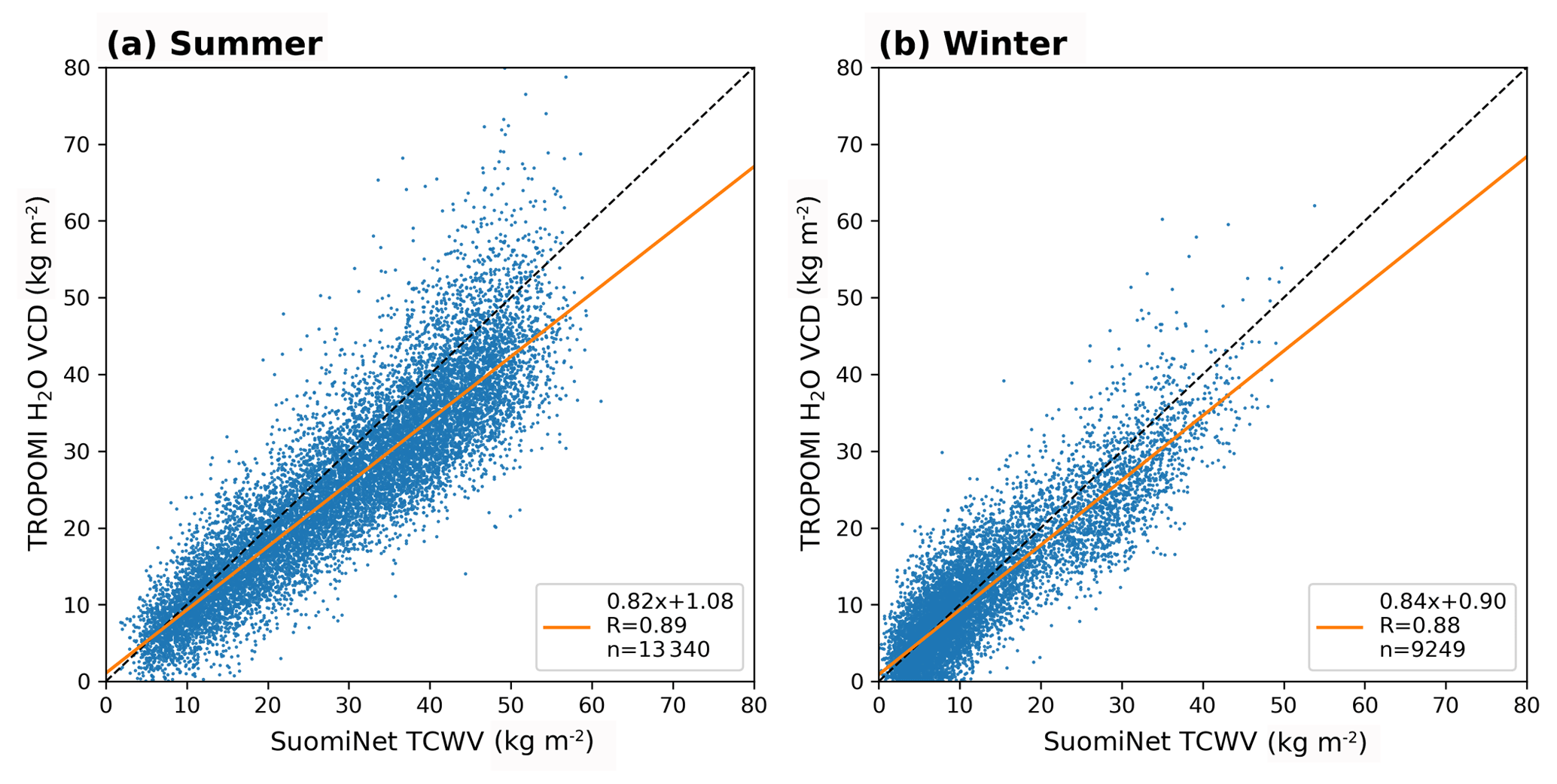
Figure 25 Scatter plots of the intercomparisons between TROPOMI and SuomiNet for clear-sky conditions (CF<20 %) for boreal summer (a) and boreal winter (b). The black dashed line indicates the 1-to-1 diagonal and the orange solid line represents the results of the robust regression based on Siegel (1982). The parameters of the regression and the coefficient of correlation are given in the box in each panel.

Figure 25 illustrates scatter plots of the intercomparison between TROPOMI and SuomiNet for boreal summer and winter. For both seasons the robust regression indicates an underestimation of around 20 % (i.e. slopes of 0.82 and 0.84) with high Pearson correlation coefficients of 88 %. In order to investigate the influence of clouds on our retrieval, we plot the difference (top row) and the relative difference (bottom row) between TROPOMI and Suominet as a function of the input cloud top height (CTH) in Fig. 26. The median over the whole CTH range (blue dashed line) indicates an underestimation of the TROPOMI H₂O VCD of approximately 14 % (3.5 kg m⁻²) during summer and of 8 % (0.8 kg m⁻²) during winter. However, during summer the median values for each 1 km CTH bin (blue dots) reveal that the underestimation is mainly caused by low clouds, whereas for mid- and high-level clouds the median difference almost cancels out. During winter this pattern is not clearly observable due to much larger scatter, but also here low clouds mainly cause the underestimation in TCWV, whereby the difference is generally within the range of accuracy of the SuomiNet retrieval.

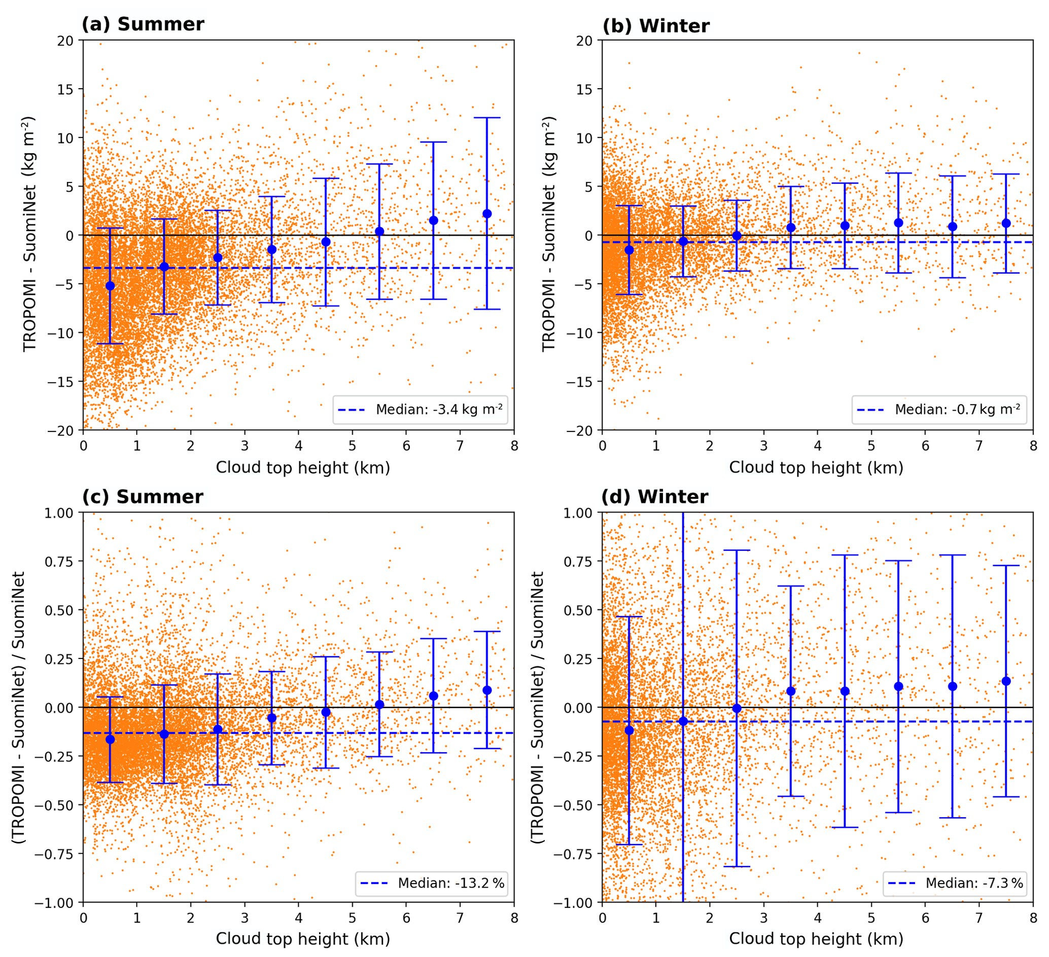
Figure 26 Scatter plot of the difference (TROPOMI − SuomiNet, a, b) and relative difference $(\mathrm{TROPOMI}-\mathrm{SuomiNet})/\mathrm{SuomiNet}$ (c, d) as a function of the input cloud top height (CTH) for clear-sky conditions (CF<20 %) for summer (a, c) and winter (b, d). The blue dashed line represents the median over the whole CTH range. The blue dots represent the median within a 1 km CTH and the error bars represent their respective 1σ standard deviation.

Figure S14 depicts further validation results separated into different cloud fraction and cloud top height bins for boreal summer 2018. Though the sample size is much smaller, similar results to SSMIS and ERA-5 are obtained: independent of the cloud fraction, low clouds cause an underestimation of around 15 %–20 %, whereas for mid-level clouds the TROPOMI H₂O VCDs show much better agreement with the SuomiNet TCWV, and for high clouds TROPOMI overestimates by around 10 %.

7 Summary and conclusions

In this paper, we introduce a total column water vapour retrieval from TROPOMI spectra in the visible blue spectral range using an iterative vertical column conversion scheme and provide a detailed characterization of our retrieved H₂O VCD by performing a detailed uncertainty analysis and intercomparisons to reference data sets from the microwave sensor SSMIS, from the reanalysis model ERA-5, and from the ground-based GPS network SuomiNet.

For the iteration scheme we describe the a priori water vapour profile as an exponential decay with a scale height H and developed an empirical parameterization for this scale height. This parameterization is based on COSMIC water vapour profile data and relates the a priori water vapour profile shape to the H₂O VCD, the seasonal cycle, the latitude, and the vegetation (and NDVI respectively). We demonstrate that we can correctly reproduce the scale heights, in particular for data at low latitudes (tropics and subtropics). However, we also observe an increasing scatter if higher latitudes are included in the comparison, likely because of the higher variability in H₂O VCD due to midlatitudinal cyclone dynamics and a general higher uncertainty in the COSMIC profile data for drier atmospheric conditions. Overall, the retrieved profile heights are very reasonable, and we obtain a substantial improvement using the new parameterization compared to the use of a prescribed constant water vapour profile.

For the uncertainty analysis we investigated the impact of several error sources on the H₂O SCD and AMF, like clouds, surface albedo, profile shape, and instrument properties. The error estimation reveals that the main SCD uncertainty is the fit error of the spectral analysis and that the main AMF uncertainties are caused by uncertainties in the surface albedo and water vapour profile shape. For the H₂O VCD we estimated a typical total relative error of around 10 %–20 % for observations during clear-sky conditions, over ocean surface, and at low solar zenith angles. For observations during cloudy-sky conditions, over land surface, and high solar zenith angles the error reaches values of approximately 20 %–50 %. Thus, the theoretically estimated errors are of the same order of magnitude as the deviations found during the retrieval's evaluation. However, uncertainties in the absorption cross section of water vapour are a further systematic error source that can additionally contribute up to 10 %. Based on the LP-DOAS comparisons we estimate these errors to be around 5 % for this study, so that they are negligible compared to the other error sources.

In the validation study we demonstrate that for clear-sky conditions the retrieved TROPOMI H₂O VCDs over ocean are in very good agreement with the reference data sets and can correctly capture the global water vapour distribution. Over land the TROPOMI retrieval can reproduce the TCWV distribution; however, we also observe a distinctive underestimation of around 10 %, in particular during boreal summer.

Nevertheless, these underestimations might be caused by the uncertainties of the external input data for the retrieval: for instance, the OMI LERs from Kleipool et al. (2008) are too high over tropical land masses, likely due to incorrect cloud filtering which causes too high AMFs, leading to too low H₂O VCDs. Although we tried to overcome this issue by using a surface reflectance product from MODIS Aqua, the cloud products from the TROPOMI L2 NO₂ product still rely on the OMI LER to calculate the effective cloud fraction and cloud top height and thus also have a large uncertainty. The intercomparisons to the reference data sets show that these uncertainties in the cloud products have a substantial impact on the H₂O VCD: our investigations reveal that the input cloud top height is probably too low, which in turn leads to higher AMFs and consequently to an underestimation in TCWV. However, one has to consider that the radiative properties of the cloud and albedo products interact at a high degree of complexity, so that a clear explanation or suggestion on how to overcome these issues is beyond the scope of this paper. Because of all these uncertainties we recommend for general purposes to only use VCDs with an effective cloud fraction <20 % and AMF>0.1, which represents a good compromise between spatial coverage and retrieval accuracy.

Overall, the successful application of the TCWV retrieval in the visible blue spectral range to TROPOMI measurements is very promising for further investigations, including application to further satellite sensors such as OMI, SCIAMACHY, and GOME-1/2 or the upcoming Sentinel-4 and Sentinel-5 instruments and expanding the retrieval to measurements contaminated by higher cloud fractions. As the retrieval allows for a fast execution of large data sets, investigations of long-term trends using a TCWV data set of merged time series of different satellite sensors are easily possible. However, since these data sets have to be uniform, they require consistent input data across the different satellite sensors, in particular for cloud products.

Appendix A: Weighted linear least-squares fit for spectral analysis

To handle the daily high data volume of TROPOMI and to avoid “jumps” of pixels included in the fit window, we implemented a weighted linear least-squares fit for the DOAS analysis. The weights W are the fractional coverage of the pixel within the fit window (see also Fig. A1):

$$\begin{array}{}\text{(A1)}& W\left(\mathit{\lambda }\right)=\left\{\begin{array}{ll}\mathrm{1}-\frac{\left|\mathit{\lambda }-{\mathit{\lambda }}_{\mathrm{low}}\right|}{\mathrm{\Delta }\mathit{\lambda }}& \frac{\left|\mathit{\lambda }-{\mathit{\lambda }}_{\mathrm{low}}\right|}{\mathrm{\Delta }\mathit{\lambda }}<\mathrm{1}\wedge \mathit{\lambda }-{\mathit{\lambda }}_{\mathrm{low}}<\mathrm{0},\\ \mathrm{1}& {\mathit{\lambda }}_{\mathrm{low}}<\mathit{\lambda }<{\mathit{\lambda }}_{\mathrm{up}}\\ \mathrm{1}-\frac{\left|\mathit{\lambda }-{\mathit{\lambda }}_{\mathrm{up}}\right|}{\mathrm{\Delta }\mathit{\lambda }}& \frac{\left|\mathit{\lambda }-{\mathit{\lambda }}_{\mathrm{up}}\right|}{\mathrm{\Delta }\mathit{\lambda }}<\mathrm{1}\wedge \mathit{\lambda }-{\mathit{\lambda }}_{\mathrm{up}}>\mathrm{0},\\ \mathrm{0}& \mathrm{else}\end{array}\right.\end{array}$$

with λ_low and λ_up the lower and upper boundaries of the fit window and Δλ the average wavelength increment within the fit window. The elements of the weight matrix are then given as $w_{ii}=\sqrt{W_{ii}\left({\mathit{\lambda }}_i\right)}$. Hence Eq. (2) can be solved by simple linear algebra:

$$\begin{array}{c}{\displaystyle }{\mathbf{y}}^{\prime }={\mathbf{M}}^{\prime }\mathbf{x},\\ {\displaystyle }\widehat{\mathbf{x}}={\left({{\mathbf{M}}^{\prime }}^T{\mathrm{M}}^{\prime }\right)}^{-\mathrm{1}}{{\mathbf{M}}^{\prime }}^T\mathbf{y},\\ {\displaystyle }\mathbf{S}={\left({{\mathbf{M}}^{\prime }}^T{\mathbf{M}}^{\prime }\right)}^{-\mathrm{1}}{\mathit{\chi }}^{\mathrm{2}},\\ {\displaystyle }{\mathit{\beta }}_i=\sqrt{S_{ii}},\end{array}$$

with the solution of the linear problem $\widehat{\mathbf{x}}$ containing the SCDs, ${\mathbf{y}}^{\prime }=\mathrm{diag}\left(\mathbf{w}\right)y$ the weighted measurement spectrum, ${\mathbf{M}}^{\prime }=\mathrm{diag}\left(\mathbf{w}\right)\mathbf{M}$ the weighted absorption structures to fit, β_i the estimated 1σ fit error of the results for each fitted parameter, and χ² the reduced chi square.

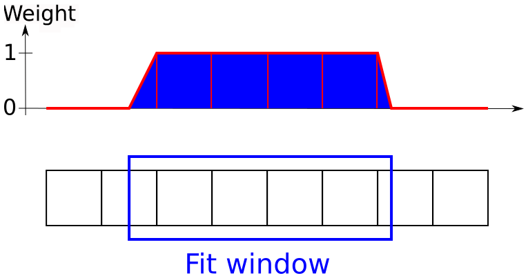
Figure A1 Schematic illustration of the weights used during the retrieval's spectral analysis.

Appendix B: Evaluation of the water vapour absorption cross section

Figure B1 depicts intercomparisons between LP-DOAS and meteorological measurements of water vapour volume mixing ratios (WVMRs) at different altitudes (10, 40, and 200 m) at the CESAR Tower for daytime and nighttime during the Cabauw Intercomparison of Nitrogen Dioxide Measuring Instruments 2 (CINDI-2) campaign. The results of the regression methods indicate that for every altitude the LP-DOAS underestimates WVMRs by around 17 % during day and 11 % during night. These findings independently confirm the results of further LP-DOAS measurements taken at the Cape Verde Atmospheric Observatory, for which Lampel et al. (2015) observed an underestimation of around 8 % when using the water vapour line lists from HITRAN 2012. However, when using the water vapour line lists from HITRAN 2008, Lampel et al. (2015) observe an excellent agreement with the reference meteorological measurements at the observatory (see Table 8 in their paper).

Figure B2 compares the absorption cross sections of the different HITRAN versions. For the high-resolution cross section (panel a), the differences between the versions are hardly visible; however, after the convolution with the TROPOMI ISRF (panel b), distinctive differences in the peak absorption are clearly visible: in comparison to HITRAN 2008, the absorption peak of HITRAN 2012 is approximately 7 %–9 % higher than HITRAN 2008, and the absorption peak of HITRAN 2016 is approximately 7 %–9 % lower than HITRAN 2008.

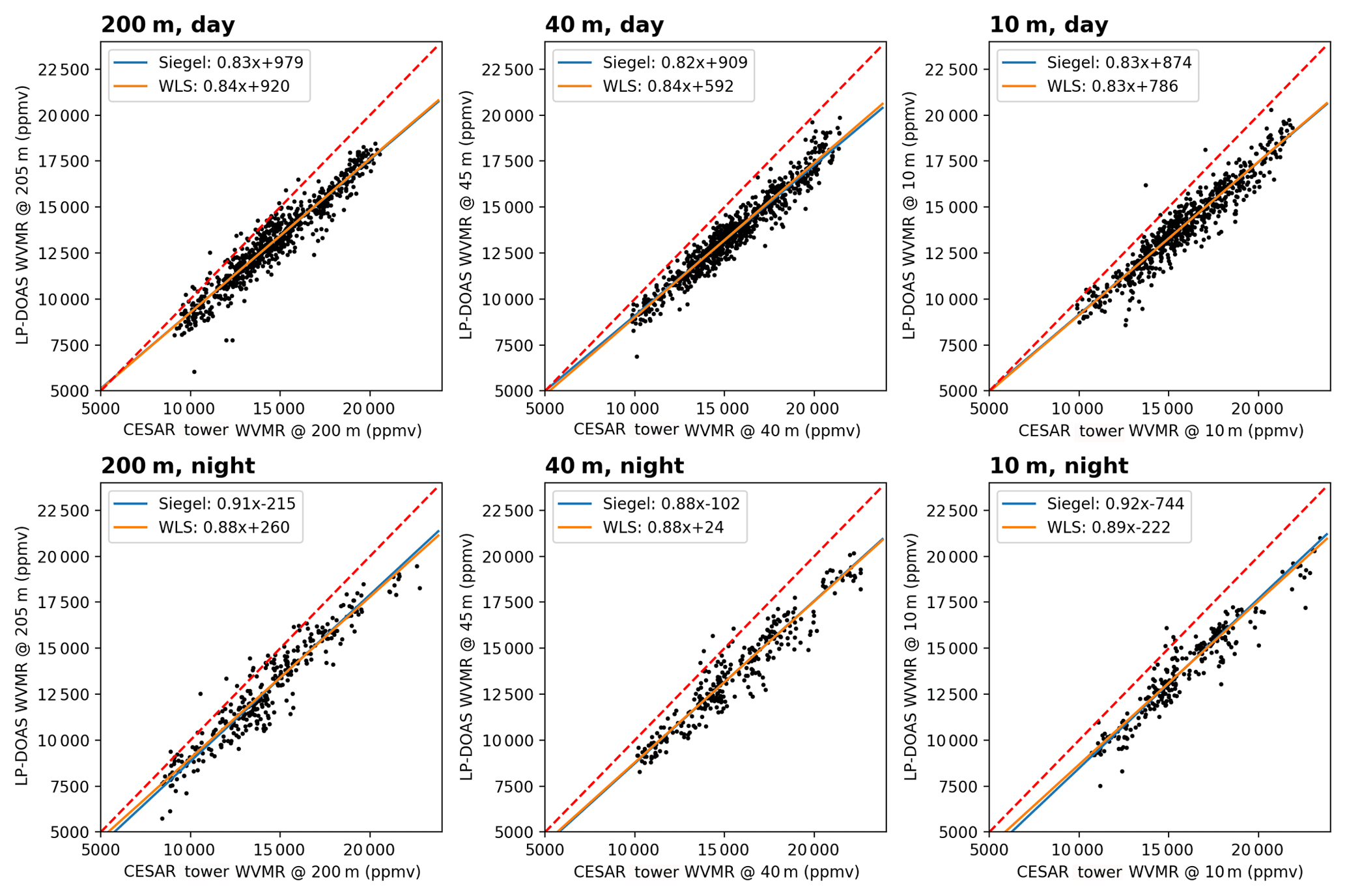
Figure B1 Scatter plots of water vapour volume mixing ratios (WVMRs) derived from LP-DOAS measurements and meteorological measurements at different altitudes (10, 40, and 200 m) at the CESAR Tower for day and night during the CINDI-2 campaign. Water vapour absorption cross sections have been calculated from the HITRAN 2012 line list. The dashed red line represents the 1-to-1 diagonal, the solid blue line the results from the robust regression (Siegel, 1982), and the solid orange line the results from the weighted linear regression.

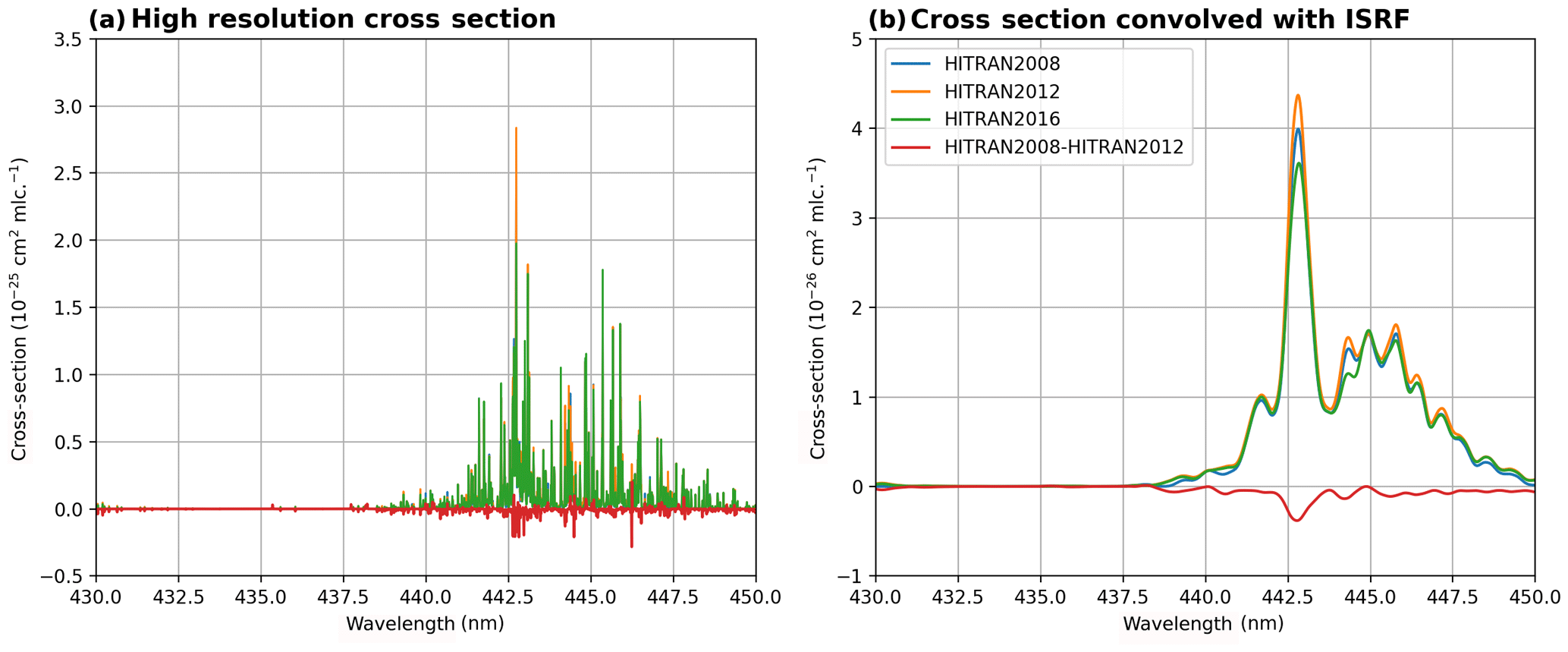
Figure B2 Comparison of the water vapour absorption cross section derived from different HITRAN versions (2008, 2012, and 2016) for a temperature of 296 K. Panel (a) depicts the high-resolution cross sections and the difference between HITRAN2008 and HITRAN2012. Panel (b) depicts the same cross sections but convolved with a typical TROPOMI Super-Gaussian ISRF (values from Beirle et al., 2017).

Combining these findings with the shortcomings of HITRAN 2016 indicated by Wang et al. (2019) and the observational evidence from the LP-DOAS measurements, we conclude that it is most adequate to use the water vapour line list from HITRAN 2008.

Appendix C: Evaluation of methods for calculating water vapour scale height

The water vapour scale height can be calculated in different ways. Here, we compare two different approaches: the first method is the calculation of the scale height via a weighted non-linear fit:

$$\begin{array}{c}{\displaystyle }min\sum _i{\displaystyle \frac{{\left(y_i-f\left(z_i,n_{\mathrm{0}},H_{\mathrm{nl}}\right)\right)}^{\mathrm{2}}}{{\mathit{\sigma }}_i^{\mathrm{2}}}}\\ {\displaystyle }f\left(z,n_{\mathrm{0}},H_{\mathrm{nl}}\right)=n_{\mathrm{0}}{e}^{-\frac{z}{H_{\mathrm{nl}}}},\end{array}$$

where y_i are the COSMIC profile data points, $f(z,n_{\mathrm{0}},H)$ is the approximation of the exponential function, and σ_i is the inverse of the layer thickness at the observation y_i. The second method consists of summing up all the partial columns of the COSMIC profile data until a defined threshold is reached, which in our case is 63 % of the H₂O VCD:

$$\begin{array}{}\text{(C1)}& {\displaystyle \frac{{\int }_{\mathrm{0}}^{H_{\mathrm{sum}}}n\left(z\right)\mathrm{d}z}{{\int }_{\mathrm{0}}^{\mathrm{TOA}}n\left(z\right)\mathrm{d}z}}>\mathrm{1}-{\displaystyle \frac{\mathrm{1}}{e}}\approx \mathrm{63}\mathit{\%}.\end{array}$$

Figure S4 depicts the mean profile shapes calculated using both methods as well as the mean profile shape of the COSMIC data for different latitude bins for the year 2013 for which the sample size is largest. Further statistics of goodness are given in Fig. S5 (bias), Fig. S6 (mean absolute error), and Fig. S7 (standard deviation). In general, the profile shapes of both methods agree well with the COSMIC measurements; however, Figs. S5 and S6 also reveal that the largest deviations occur in the lowermost troposphere, in particular for the southern polar regions. Nevertheless, the profiles of standard deviations in Fig. S7 also demonstrate that both methods are able to well capture the vertical and temporal variations in the water vapour profile shape and that these variations are within the same range of the variation of the COSMIC profile data.

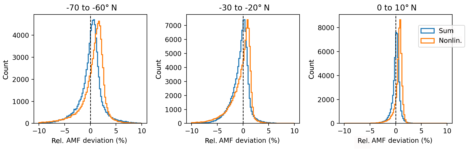
Figure C1 Histogram of the relative deviation of the calculated synthetic AMFs between the sum method (blue)/non-linear fit (orange) and the COSMIC profile for selected latitude bins (0 to 10, −30 to −20, and −70 to −60^∘ N) assuming clear-sky conditions and nadir-viewing geometry.

Figure C1 depicts histograms of the relative AMF deviation for both methods for selected latitude regions assuming nadir-viewing geometry and clear-sky conditions (like in Sect. 3.2 and Fig. 5). The peaks of the histograms for the sum method are close to the 0 % line, indicating very good agreement with AMF calculated from the COSMIC profiles. In contrast, the histograms for the non-linear fit peak at values around 2 % and show a broader distribution than the histogram of the sum method, thus revealing an inferior agreement with the reference AMFs. For cloudy-sky conditions (see Fig. S8), both methods are biased to smaller AMF values (deviations of around −5 %) for a cloud top height of 1 km, but for higher clouds both methods show similar good agreement with the reference AMFs. However, the variance in the AMFs for the sum method is much smaller than in the AMFs for the non-linear fit.

In summary, the sum method is to be preferred because it provides more consistent results for clear-sky and cloudy-sky scenarios than the non-linear fit.