Observation of sensible and latent heat flux profiles with lidar

We present the first measurement of the sensible heat flux (H) profile in the convective boundary layer (CBL) derived from the covariance of collocated vertical-pointing temperature rotational Raman lidar and Doppler wind lidar measurements. The uncertainties of the H measurements due to instrumental noise and limited sampling are also derived and discussed. Simultaneous measurements of the latent heat flux profile (L) and other turbulent variables were obtained with the combination of water-vapor differential absorption lidar (WVDIAL) and Doppler lidar. The case study uses a measurement example from the HOPE (HD(CP)² Observational Prototype Experiment) campaign, which took place in western Germany in 2013 and presents a cloud-free well-developed quasi-stationary CBL. The mean boundary layer height z_i was at 1230 m above ground level. The results show – as expected – positive values of H in the middle of the CBL. A maximum of (182±32) W m⁻², with the second number for the noise uncertainty, is found at 0.5 z_i. At about 0.7 z_i, H changes sign to negative values above. The entrainment flux was $(-\mathrm{62}\pm \mathrm{27})$ W m⁻². The mean sensible heat flux divergence in the observed part of the CBL above 0.3 z_i was −0.28 W m⁻³, which corresponds to a warming of 0.83 K h⁻¹. The L profile shows a slight positive mean flux divergence of 0.12 W m⁻³ and an entrainment flux of (214±36) W m⁻². The combination of H and L profiles in combination with variance and other turbulent parameters is very valuable for the evaluation of large-eddy simulation (LES) results and the further improvement and validation of turbulence parameterization schemes.

1 Introduction

The energy reaching the earth surface in form of solar radiation during the daytime is partly reflected as outgoing radiation, partly conducted into the ground and partly transported into the atmosphere by turbulent eddies of various scales forming the convective boundary layer (CBL) during the daytime (LeMone, 2002). The latter energy flux partitions into sensible heat flux H and latent heat flux L. The understanding of H and L profiles is decisive for correct atmospheric simulations with models since these profiles rule the heat and water budgets, the distribution of humidity and temperature, and thus the atmospheric stability and furthermore the formation of clouds and precipitation.

The variance of humidity and temperature at the CBL top determines cloud formation (Moeng and Sullivan, 1994). Weckwerth et al. (1996) found strong variability in the moisture structure in the CBL due to the presence of horizontal convective rolls. The coherent perturbations of temperature and moisture in these rolls influence the formation of deep convection (Weckwerth et al., 1999). Also, surface flux partitioning is an important parameter for studying convection initiation (e.g., Gantner and Kalthoff, 2010; Adler et al., 2011; Behrendt et al., 2011; Kalthoff et al., 2011) and land–atmosphere feedback (Santanello et al., 2018). Clearly, not only the mean structure of moisture in the CBL is important but also the variance profiles due to their contribution to the variance budget (Lenschow et al., 1980). At the same time, variations in the humidity structure also influence precipitation patterns (Dierer et al., 2009).

It is difficult to parameterize these sub-grid-scale moisture variations in cloud, convection, and turbulence-resolving models (Moeng and Sullivan, 1994). Shallow cumulus parameterizations (e.g., Bretherton and Park, 2009; Neggers, 2009; Berg et al., 2013) are used in mesoscale models which do not resolve the turbulent eddies to approximate their effects. These schemes are decisive for the correct simulation of clouds and precipitation. To verify these parameterizations in weather prediction models, not only monitoring of the mean CBL thermodynamic structure (e.g., Milovac et al., 2016), but also measurements of higher-order moments of turbulent fluctuations of the thermodynamic variables (like variances, skewness, kurtosis) and their covariances (like H and L) are highly desirable (e.g., Ayotte et al., 1996; Heinze et al., 2017; Osman et al., 2019). Preferably, these parameters should be collected continuously in time and simultaneously throughout the CBL.

It is clear that in situ measurements performed from airborne platforms (e.g., Grunwald et al., 1996, 1998; Bange et al., 2002) can only sample the atmosphere stepwise. Recently unmanned aerial vehicle systems were used for the estimation of water-vapor fluxes in the CBL (Thomas et al., 2012). However, in situ measurement systems cannot obtain the total vertical profile simultaneously and continuously over longer measurement periods, though it is very important to derive the flux divergence.

In recent years, it has been demonstrated that lidar, a laser remote-sensing technique covering the CBL, is capable of not only determining mean profiles and gradients in the daytime CBL, the interfacial layer, and the lower free troposphere above but also higher-order-moment profiles of turbulent fluctuations for more and more variables: vertical wind (e.g., Frehlich et al., 1998; Lenschow et al., 2000, 2012; Lothon et al., 2006, 2009; Hogan et al., 2009; O'Connor et al., 2010; Lenschow et al., 2012), humidity (Kiemle et al., 1997; Wulfmeyer, 1999a; Wulfmeyer et al., 2010; Lenschow et al., 2000; Couvreux et al., 2005, 2007; Turner et al., 2014a, b; Muppa et al., 2016; Di Girolamo et al., 2017), aerosol backscatter (Pal et al., 2010), and – most recently – also temperature (Behrendt et al., 2015; Di Girolamo et al., 2017). Consequently, large-eddy-simulation (LES) models can be evaluated with the synergy of temperature, humidity, and wind lidar systems (Heinze et al., 2017) and new parameterizations can be developed (Wulfmeyer et al., 2016, 2018).

First measurements of virtual heat flux with a remote-sensing technique, were presented by Peters et al. (1985) by combining a sodar for vertical wind measurements and a radio acoustic sounding system (RASS) for virtual temperature measurements reaching heights of up to 188 m above ground level (a.g.l.). With the combination of a radar wind profiler and a RASS, the range of virtual heat flux measurements could later be extended up to a few hundred meters (Angevine et al., 1993a), and comparisons with aircraft measurements were made for the average of a 7 d period reaching up to 0.8 z_i, with z_i being the CBL height (Angevine et al., 1993b). Since RASS measures the virtual temperature and not the physical temperature (Matuura et al., 1986), the measured virtual heat flux depends also on humidity fluctuations. For model comparisons, however, separate measurements of H and L are preferable.

First L measurements in the CBL with remote-sensing techniques were achieved by Senff et al. (1994) with a combination of water-vapor differential absorption lidar (WVDIAL) and RASS. Heights between 400 and 700 m a.g.l. could be investigated. Wulfmeyer (1999b) used the same combination of techniques at a site located at the coast of the island of Gotland, Sweden, even reaching heights beyond z_i with about the same range at that site . The first lidar-only flux measurements were made by Giez et al. (1999) by combining WVDIAL and Doppler lidar for L profiling. Because the range of Doppler lidar is larger than the range of RASS, the authors extended the range of lidar L profiles to about 1300 m a.g.l. with this approach. The same combination of lidar systems was also applied by Linné et al. (2007). Kiemle et al. (2007, 2011) operated the technique from an airborne platform over flat and complex terrain. The first water-vapor flux profiling using a Raman lidar and a Doppler lidar was demonstrated in Wulfmeyer et al. (2018) showing a good performance with respect to statistical errors.

While all the abovementioned measurements were made in the CBL – which means in the daytime – Rao et al. (2002) presented nighttime water-vapor Raman lidar measurements in combination with sodar measurements estimating L profiles in the nocturnal urban boundary layer under unstable conditions.

Lidar flux measurements of other trace gases than water vapor were discussed, e.g., by Senff et al. (1996), who combined an ozone DIAL and a RASS for measuring turbulent ozone fluxes, and by Gibert et al. (2011), who combined a CO₂ DIAL and Doppler lidar for measuring turbulent CO₂ fluxes. Profiles of turbulent aerosol particle mass fluxes in the CBL were measured by Engelmann et al. (2008) with a combination of aerosol Raman lidar and Doppler lidar.

While there has been great progress for measuring all these different types of fluxes in the atmospheric boundary layer in recent years, profiles of H – highly desirable for model verification – were not available to date due to the lack of suitable remote-sensing temperature measurements with high temporal and spatial resolution in the daytime CBL. In the following, we will show that this gap has been closed with temperature rotational Raman lidar (TRRL). This technique (see, e.g., Behrendt, 2005, for an overview) provides the physical temperature of the atmosphere independent of assumptions on the atmospheric state (like hydrostatic equilibrium) and other parameters like humidity or aerosol particle density. In contrast to the virtual heat flux measurements obtained with RASS, TRRL provides data for the heat flux and not the virtual heat flux, the latter of which is entangled with L. In recent years, the TRRL technique achieved precise measurements not only at night but also in the daytime reaching heights up to the CBL top and above into the lower free troposphere (e.g., Radlach et al., 2008; Hammann et al., 2015; Behrendt et al., 2015; Di Girolamo et al., 2017; Lange et al., 2019). This was challenging because of the relatively low backscatter cross section of the inelastic Raman backscatter processes combined with low temperature sensitivity. Key for the achievement were powerful ultraviolet lasers in combination with more efficient receiver designs. Furthermore, the calibration function of TRRL systems must be stable, which means that technical solutions had to be implemented so that neither the laser wavelength nor the optical properties of the receiver components vary.

An overview of the instruments is given in Sect. 2. The methodology is described in Sect. 3. The results are presented and discussed in Sect. 4. Finally, a summary and an outlook are given.

2 Instruments

2.1 Temperature rotational Raman lidar

Rotational Raman lidar makes use of Raman signals of atmospheric molecules (mainly N₂ and O₂) of different temperature dependencies (Cooney, 1972; Behrendt, 2005). From the ratio of the atmospheric backscatter signals, a measurement signal is obtained which depends on atmospheric temperature. The rotational Raman lidar of the University of Hohenheim was designed with the focus on high-resolution measurements during the daytime (Radlach et al., 2008; Hammann et al., 2015; Hammann and Behrendt, 2015). As a laser transmitter, a frequency-tripled injection-seeded Nd:YAG laser is used (see also Di Girolamo et al., 2004), which emits 200 mJ laser pulses at 355 nm with a repetition rate of 50 Hz. A Pellin–Broca prism refracts the other laser wavelengths out of the optical path, which makes the system eye-safe from short distances onward. The whole lidar is housed in a truck so that it can be moved easily to field campaigns. A two-mirror scanner allows for three-dimensional observations. For the measurements discussed here, this scanner was pointing vertically. The backscatter signals of the atmosphere are collected with a telescope with a 40 cm primary mirror and then separated with interference filters into four channels: the elastic channel, two rotational Raman channels, and a water-vapor Raman channel. The first three of these channels are mounted in a cascade, which makes the signal separation very efficient (Behrendt and Reichardt, 2000; Behrendt et al., 2002, 2004). The water-vapor Raman channel was not yet in operation for the measurements discussed here, but the beam splitter for this channel was already in place. Photomultipliers collect the four signals and give electric signals, which are analyzed with a combined photon-counting and analog transient recorder (LICEL GmbH). A temporal resolution of 10 s and a range resolution of 3.75 m were selected for the raw data of all channels. For the temperature measurements, the two rotational Raman signals were first smoothed with a gliding average of 108.75 m; then the ratio of the signals was calculated. For the temperature calibration, data of a radiosonde launched at the lidar site were used. The second-order logarithmical function suggested by Behrendt and Reichart (2000) was used as calibration function. Since the strong daytime photon-counting signals were influenced by dead-time effects in the ranges discussed in this study, we used only analog signals.

2.2 Doppler wind lidar

Doppler lidar measures the radial wind velocity via the Doppler shift of laser radiation scattered in the atmosphere (e.g., Werner, 2005). In this study, we used data of the heterodyne Doppler lidar Wind-Tracer WTX of Lockheed Martin Coherent Technologies, USA, operated by the Karlsruhe Institute of Technology (KIT) (Träumner et al., 2014). The lidar transmitter is a Er:YAG laser that emits laser pulses at a wavelength of 1.6 µm using a pulse repetition frequency of 750 Hz with 2.7 mJ pulse energy. The lidar can be operated in different scan patterns. Vertical stare mode yields vertical velocity w with a time resolution of typically 1 s from about 375 m a.g.l. to the top of the boundary layer and partly above, depending mainly on the aerosol concentration. The effective range-gate resolution was about 60 m.

2.3 Water-vapor differential absorption lidar

In the following, we also introduce briefly the WVDIAL of the University of Hohenheim (UHOH) because we show latent heat flux profiles for comparison. WVDIAL provides absolute humidity profiles with high temporal and spatial resolution in the lower troposphere (Wulfmeyer and Bösenberg, 1998). During the HOPE campaign (see Sect. 4.1 below for definition; Macke et al., 2017), the scanning water-vapor WVDIAL of the University of Hohenheim (Wagner et al., 2013) was operated in vertical mode during clear-sky conditions and in scanning mode during cloudy periods (Späth et al., 2016). The operational wavelength of the UHOH WVDIAL is near 818 nm. The laser transmitter was switched shot by shot between the online and offline frequencies. The backscatter signals were recorded for each laser shot (250 Hz) with a range resolution of 15 m. The measured absolute humidity has typical temporal and spatial resolutions of 1 s to 1 min and 15 to 300 m, respectively, depending on the range of interest. Due to the instrument's high laser power (about 2 W) in combination with a very efficient receiver (0.8 m telescope), the data have low noise uncertainties up to the CBL top. When deriving absolute humidity from the UHOH WVDIAL data used in this study, 10 s averages and a gliding window length of 135 m for the Savitzky–Golay algorithm (Savitzky and Golay, 1964) were used, resulting in a triangular weighting function with a full width at half maximum of about 60 m.

3 Methodology

3.1 Sensible and latent heat flux analyses

Lenschow et al. (2000) introduced a procedure for the estimation of higher-order moments of turbulent fluctuations that accounts for random instrumental noise. We follow this method for resolving the turbulent moments of temperature, vertical wind, and humidity for estimating instrument noise uncertainties. Further, important refinements were presented in Wulfmeyer et al. (2016) such as automated spike detection and the proper choice of lags used in the autocovariance analyses.

The flux profiles in the CBL were calculated using the eddy covariance method (see, e.g., Senff et al., 1994; Wulfmeyer, 1999b). The data processing procedure is described in detail in Wulfmeyer et al. (2016). In the following, we explain the method with the sensible heat flux as an example; the measurement of the latent heat flux works in an analogous way. First, temperature and wind data measured by the TRRL and Doppler lidar, respectively, were despiked. This means that histograms of the data at each height were calculated for the selected period, and then all data outside of 4 standard deviations from the median were removed. Other authors (Turner et al., 2014a, b) refined the despiking of noisy lidar data by also considering non-Gaussian distributions and asymmetric despiking thresholds on either side of the histogram, but we found that for the case shown here such further refinements do not change the results significantly. A despiking procedure is required because the lidar data analysis algorithms are non-linear and noise in the data may result in large (non-linear) outliers in some cases.

In a second step, the despiked temperature data were detrended using a linear fit at each height level. This procedure is required in order to focus on the turbulent fluctuations by removing influences of large-scale advection, synoptic processes, and the diurnal cycle. Detrending means that the time series of the scalar observations s(z, t), with s being, e.g., temperature T or humidity q, z being height above ground, and t being time, are used over the selected period to obtain mean linear trends $s^{*}(z,t)$ and that these trends were then subtracted from the instantaneous values s(z, t) at each height to obtain the fluctuations

$$\begin{array}{}\text{(1)}& s{}^{\prime }(z,t)=s(z,t)-s^{*}(z,t).\end{array}$$

Consequently, the mean of these fluctuations becomes zero.

In case of the wind data w(z, t), we decided to subtract only time-independent means at each height level of the vertical wind data in order to ensure fluctuations with perfect zero mean. Detrending alters the real atmospheric fluctuations quite significantly when the updrafts and downdrafts are not perfectly evenly distributed in the analysis period (which is in practice never the case due to the statistical nature of the thermals in the CBL).

In practice, both despiking and detrending has to be performed with caution in order not to eliminate real atmospheric features. This means that the time series of data should be investigated first and only quasi-stationary time series with small trends in the scalar (T or q), small biases in w, and a sufficient number of thermals should be used in order to obtain fluxes with low systematic errors. Typically, the time period for the analysis thus need to be at least 30 min.

Before the scalar and wind time series can be combined, one must ensure in a third step that the time and height for each data point are as close as possible. For this, we gridded the data to closest neighbors.

The correlation of the temperature fluctuations T^′ and the vertical wind fluctuations w^′ provides profiles of the eddy sensible heat flux according to

$$\begin{array}{}\text{(2)}& H\left(z\right)={\mathit{\rho }}_{\mathrm{a}}\left(z\right)c_p\stackrel{\mathrm{‾}}{w{}^{\prime }\left(z\right)T{}^{\prime }\left(z\right)},\end{array}$$

with ρ_a(z) for the air density at height z and c_p for the specific heat capacity of air.

For the lidar data, which are discrete in time, Eq. (2) results in

$$\begin{array}{}\text{(3)}& H\left(z\right)={\displaystyle \frac{{\mathit{\rho }}_{\mathrm{a}}\left(z\right)c_p}{N\left(z\right)}}\sum _{i=\mathrm{1}}^{N\left(z\right)}w{{}^{\prime }}_i\left(z\right)T{{}^{\prime }}_i\left(z\right),\end{array}$$

where i is the number of each data point and N(z) is the total number of common data points at height z of T^′ and w^′. N(z) is not the same for all heights z because the despiking routine removes a few data points.

3.2 Uncertainties due to noise and representativeness

The instrumental noise uncertainty and the representativeness uncertainty play a major role when deriving the statistics of turbulent fluctuations in the atmosphere with noisy data (Lenschow et al., 1994, 2000). The noise uncertainty is due to the instrumental noise of the lidar data. The uncertainty due to sampling only a limited period of time covering a limited number of turbulent eddies is referred to as representativeness uncertainty or sampling uncertainty.

Fortunately, when H(z) is calculated with the lidar data with Eq. (3), the noise contributions of the vertical wind and temperature fluctuations, $w{{}^{\prime }}_{\mathrm{i},\mathrm{n}}\left(z\right)$ and $T{{}^{\prime }}_{\mathrm{i},\mathrm{n}}\left(z\right)$, do not cause a bias in the covariance and – unlike for the variances – no subtraction of an instrumental noise term is required.

This can be understood by splitting the fluctuations into an atmospheric part and into a noise part according to

$$\begin{array}{}\text{(4)}& w{{}^{\prime }}_{\mathrm{i}}\left(z\right)=w{{}^{\prime }}_{\mathrm{i},\mathrm{a}}\left(z\right)+w{{}^{\prime }}_{\mathrm{i},\mathrm{n}}\left(z\right)\end{array}$$

and

$$\begin{array}{}\text{(5)}& T{{}^{\prime }}_{\mathrm{i}}\left(z\right)=T{{}^{\prime }}_{\mathrm{i},\mathrm{a}}\left(z\right)+T{{}^{\prime }}_{\mathrm{i},\mathrm{n}}\left(z\right).\end{array}$$

Inserting Eqs. (4) and (5) in Eq. (3) yields

$$\begin{array}{}\text{(6)}& \begin{array}{rl}H\left(z\right)& ={\displaystyle \frac{{\mathit{\rho }}_{\mathrm{a}}\left(z\right)c_p}{N\left(z\right)}}\sum _{i=\mathrm{1}}^{N\left(z\right)}\left(w{{}^{\prime }}_{\mathrm{i},\mathrm{a}}\right(z\left)T{{}^{\prime }}_{\mathrm{i},\mathrm{a}}\right(z)+w{{}^{\prime }}_{\mathrm{i},\mathrm{a}}(z\left)T{{}^{\prime }}_{\mathrm{i},\mathrm{n}}\right(z)\\ & +w{{}^{\prime }}_{\mathrm{i},\mathrm{n}}\left(z\right)T{{}^{\prime }}_{\mathrm{i},\mathrm{a}}\left(z\right)+w{{}^{\prime }}_{\mathrm{i},\mathrm{n}}\left(z\right)T{{}^{\prime }}_{\mathrm{i},\mathrm{n}}\left(z\right))\end{array},\end{array}$$

and hence

$$\begin{array}{}\text{(7)}& H\left(z\right)={\displaystyle \frac{{\mathit{\rho }}_{\mathrm{a}}\left(z\right)c_p}{N\left(z\right)}}\sum _{i=\mathrm{1}}^{N\left(z\right)}w{{}^{\prime }}_{\mathrm{i},\mathrm{a}}\left(z\right)T{{}^{\prime }}_{\mathrm{i},\mathrm{a}}\left(z\right)\end{array}$$

because $w{{}^{\prime }}_{\mathrm{i},\mathrm{n}}\left(z\right)$ and $T{{}^{\prime }}_{\mathrm{i},\mathrm{n}}\left(z\right)$ are uncorrelated with each other as well as with the atmospheric fluctuations.

But even though there is no noise term to be subtracted when determining fluxes from noisy data, of course, there still remains an uncertainty of the flux value due to noise: because the real atmospheric data set is always of a finite length, the noise terms do not cancel fully. This noise uncertainty of the covariance of the fluctuations of a scalar s (e.g., T or q) and the vertical wind w can be estimated by applying Gaussian error propagation to Eq. (7) giving (Wulfmeyer et al., 2016)

$$\begin{array}{}\text{(8)}& {\mathit{\sigma }}_{\stackrel{\mathrm{‾}}{w{}^{\prime }s{}^{\prime }}}\left(z\right)\cong \sqrt{{\displaystyle \frac{\stackrel{\mathrm{‾}}{s{{}^{\prime }}_{\mathrm{a}}(z{)}^{\mathrm{2}}}{\mathit{\sigma }}_{w{}^{\prime }}(z{)}^{\mathrm{2}}+\stackrel{\mathrm{‾}}{w{{}^{\prime }}_{\mathrm{a}}(z{)}^{\mathrm{2}}}{\mathit{\sigma }}_{s{}^{\prime }}(z{)}^{\mathrm{2}}}{N\left(z\right)}}},\end{array}$$

with ${\mathit{\sigma }}_{w{}^{\prime }}(z{)}^{\mathrm{2}}$ and ${\mathit{\sigma }}_{s{}^{\prime }}(z{)}^{\mathrm{2}}$ for the noise variances of the scalar and the vertical wind at height z, respectively. Furthermore, the noise uncertainties of the fluctuations are equal to the noise uncertainties of the original (non-detrended) data sets – ${\mathit{\sigma }}_{w{}^{\prime }}(z{)}^{\mathrm{2}}={\mathit{\sigma }}_w(z{)}^{\mathrm{2}}$ and ${\mathit{\sigma }}_{s{}^{\prime }}(z{)}^{\mathrm{2}}={\mathit{\sigma }}_s(z{)}^{\mathrm{2}}$ (assuming that the noise uncertainty in the trend determination can be neglected); nevertheless, in the following we keep the notation with primes for clarity as we are dealing with fluctuations here.

Equation (8) can be further approximated and rearranged so that the relative noise of the covariance is expressed with the relative noise variances according to

$$\begin{array}{}\text{(9)}& {\displaystyle \frac{{\mathit{\sigma }}_{\stackrel{\mathrm{‾}}{w{}^{\prime }s{}^{\prime }}}}{\stackrel{\mathrm{‾}}{w{}^{\prime }s{}^{\prime }}}}\cong \sqrt{{\displaystyle \frac{\mathrm{1}}{N{r}^{\mathrm{2}}}}\left({\displaystyle \frac{{\mathit{\sigma }}_{s^{\prime }}^{\mathrm{2}}}{\stackrel{\mathrm{‾}}{s{{}^{\prime }}_{\mathrm{a}}^{\mathrm{2}}}}}+{\displaystyle \frac{{\mathit{\sigma }}_{w^{\prime }}^{\mathrm{2}}}{\stackrel{\mathrm{‾}}{w{{}^{\prime }}_{\mathrm{a}}^{\mathrm{2}}}}}\right)},\end{array}$$

where r is the correlation coefficient between atmospheric vertical wind fluctuations and atmospheric scalar fluctuations given by

$$\begin{array}{}\text{(10)}& r={\displaystyle \frac{\stackrel{\mathrm{‾}}{w{}^{\prime }s{}^{\prime }}}{\sqrt{\stackrel{\mathrm{‾}}{w{{}^{\prime }}_{\mathrm{a}}^{\mathrm{2}}}\stackrel{\mathrm{‾}}{s{{}^{\prime }}_{\mathrm{a}}^{\mathrm{2}}}}}}.\end{array}$$

Please note that we omit the height dependence for simplicity in Eq. (9) and the following equations. Consequently, it follows for the noise uncertainty of the sensible heat flux that

$$\begin{array}{}\text{(11)}& {\displaystyle \frac{{\mathit{\sigma }}_{\mathrm{H}}}{H}}\cong \sqrt{{\displaystyle \frac{\mathrm{1}}{N{r}^{\mathrm{2}}}}\left({\displaystyle \frac{{\mathit{\sigma }}_{T^{\prime }}^{\mathrm{2}}}{\stackrel{\mathrm{‾}}{T{{}^{\prime }}_{\mathrm{a}}^{\mathrm{2}}}}}+{\displaystyle \frac{{\mathit{\sigma }}_{w^{\prime }}^{\mathrm{2}}}{\stackrel{\mathrm{‾}}{w{{}^{\prime }}_{\mathrm{a}}^{\mathrm{2}}}}}\right)}.\end{array}$$

It is important to note that we find the variances of the atmospheric fluctuations of temperature and vertical wind in Eq. (11) but not the variances of the total fluctuations (which include both the atmospheric and noise fluctuations).

In order to identify these atmospheric variances of the temperature and vertical wind fluctuations, we use the method of Lenschow et al. (2000) to separate the noise variance from the total variance: the atmospheric variance ${\mathit{\sigma }}_{\mathrm{a}}^{\mathrm{2}}$ is obtained from the total variance ${\mathit{\sigma }}_{\mathrm{tot}}^{\mathrm{2}}$ by subtracting the noise variance ${\mathit{\sigma }}_{\mathrm{n}}^{\mathrm{2}}$:

$$\begin{array}{}\text{(12)}& {\mathit{\sigma }}_{\mathrm{a}}^{\mathrm{2}}={\mathit{\sigma }}_{\mathrm{tot}}^{\mathrm{2}}-{\mathit{\sigma }}_{\mathrm{n}}^{\mathrm{2}}.\end{array}$$

${\mathit{\sigma }}_{\mathrm{n}}^{\mathrm{2}}$ is determined from an autocovariance analysis of the high-resolution time series of the lidar data. The autocovariance at zero lag is the sum of the atmospheric and noise variances. While the atmospheric fluctuations are correlated in time, the random instrumental noise fluctuations are not. Consequently, one can separate the atmospheric variance from the noise variance by extrapolating the fit of the autocovariance function (also called “structure function”) to lag zero. The most suitable choice for the lag is a factor of 2.5 larger than the integral timescale (Wulfmeyer et al., 2016).

After the noise uncertainty profiles have been determined from the variance analysis for both the temperature and vertical wind measurements, ${\mathit{\sigma }}_{T^{\prime }}^{\mathrm{2}}$ and ${\mathit{\sigma }}_{w^{\prime }}^{\mathrm{2}}$ are used for calculating the noise uncertainty of the fluxes with Eq. (11).

The representativeness uncertainty or sampling uncertainty of the flux expressed as a variance is the square of the difference of the mean flux 〈F〉 measured in the sampled time period and the real mean flux $\stackrel{\mathrm{‾}}{F}$ which would be determined in an infinitely long measurement period:

$$\begin{array}{}\text{(13)}& {\mathit{\sigma }}_F^{\mathrm{2}}=\langle (\stackrel{\mathrm{‾}}{F}-\langle F\rangle {)}^{\mathrm{2}}\rangle .\end{array}$$

This uncertainty can be estimated for τ≫τ_ws with (Lenschow et al., 1994)

$$\begin{array}{}\text{(14)}& {\mathit{\sigma }}_{\mathrm{F}}=\sqrt{\mathrm{2}{\left(\mathrm{1}+{\displaystyle \frac{\mathrm{1}}{r^{\mathrm{2}}}}\right)}^{\mathrm{2}}{\displaystyle \frac{{\mathit{\tau }}_{\mathrm{ws}}}{\mathit{\tau }}}{\stackrel{\mathrm{‾}}{F}}^{\mathrm{2}}},\end{array}$$

where τ_ws is the integral timescale of the vertical flux of the scalar s, τ is the length of the measurement period, and r is again the correlation coefficient of s^′ and w^′. (Note that Lenschow et al., 1994, call this type of uncertainty “random error” which must not be confused with the noise uncertainty due to random noise.)

An upper limit of the representativeness uncertainty can be obtained from the minimum of the integral timescales of vertical wind τ_w and the integral timescale of the scalar τ_s via (Lenschow and Kristensen, 1985)

$$\begin{array}{}\text{(15)}& {\mathit{\sigma }}_{\mathrm{F}}=\sqrt{{\displaystyle \frac{\mathrm{4}}{r^{\mathrm{2}}}}{\displaystyle \frac{min\left({\mathit{\tau }}_{\mathrm{w}},{\mathit{\tau }}_{\mathrm{s}}\right)}{\mathit{\tau }}}{\stackrel{\mathrm{‾}}{F}}^{\mathrm{2}}}.\end{array}$$

Thus, it follows for the sensible heat flux that

$$\begin{array}{}\text{(16)}& {\mathit{\sigma }}_{\mathrm{H},\mathrm{sampling}}={\displaystyle \frac{\mathrm{2}H}{r}}\sqrt{{\displaystyle \frac{min\left({\mathit{\tau }}_{\mathrm{w}},{\mathit{\tau }}_{\mathrm{s}}\right)}{\mathit{\tau }}}}.\end{array}$$

3.3 Flux divergence and tendency

The vertical divergence of the sensible heat flux can be related to a temperature tendency via

$$\begin{array}{}\text{(17)}& {\displaystyle \frac{\mathrm{1}}{{\mathit{\rho }}_{\mathrm{a}}{c}_{\mathrm{p}}}}{\displaystyle \frac{\partial H}{\partial z}}={\displaystyle \frac{\partial \left(\stackrel{\mathrm{‾}}{w{}^{\prime }T{}^{\prime }}\right)}{\partial z}}=-{\left({\displaystyle \frac{\partial \stackrel{\mathrm{‾}}{\mathit{\theta }}}{\partial t}}\right)}_{\mathrm{FluxDiv}}.\end{array}$$

The temperature tendency term on the right-hand side of Eq. (17) is just a fraction of the total tendency, namely the contribution of the vertical flux divergence to the total tendency. We indicate this relation by the subscript FluxDiv. The tendency contributions of advection, radiative cooling, etc., are not included and need to be determined separately.

With the lidar data, we obtain the fluxes in the lower part of the CBL and at the CBL top simultaneously. Thus, we get the temperature trend due to flux divergence in the observed part of the CBL with

$$\begin{array}{}\text{(18)}& {\left({\displaystyle \frac{\partial \stackrel{\mathrm{‾}}{\mathit{\theta }}}{\partial t}}\right)}_{\mathrm{FluxDiv}}=-{\displaystyle \frac{\mathrm{1}}{{\mathit{\rho }}_{\mathrm{a}}{c}_{\mathrm{p}}}}{\displaystyle \frac{H\left(z_{\mathrm{i}}\right)-H\left(z_{\mathrm{bottom}}\right)}{z_{\mathrm{i}}-z_{\mathrm{bottom}}}},\end{array}$$

where z_bottom stands for the lowest observed height of the CBL.

In a similar way, the divergence of the latent heat flux is related to the moisture tendency in the CBL via

$$\begin{array}{}\text{(19)}& {\displaystyle \frac{\mathrm{1}}{L_{\mathrm{v}}}}{\displaystyle \frac{\partial L}{\partial z}}={\displaystyle \frac{\partial \left(\stackrel{\mathrm{‾}}{w{}^{\prime }q{}^{\prime }}\right)}{\partial z}}=-{\left({\displaystyle \frac{\partial \stackrel{\mathrm{‾}}{q}}{\partial t}}\right)}_{\mathrm{FluxDiv}}.\end{array}$$

with L_v for the latent heat of vaporization and thus for the lidar data we use

$$\begin{array}{}\text{(20)}& {\left({\displaystyle \frac{\partial \stackrel{\mathrm{‾}}{q}}{\partial t}}\right)}_{\mathrm{FluxDiv}}=-{\displaystyle \frac{\mathrm{1}}{L_{\mathrm{v}}}}{\displaystyle \frac{L\left(z_{\mathrm{i}}\right)-L\left(z_{\mathrm{bottom}}\right)}{z_{\mathrm{i}}-z_{\mathrm{bottom}}}}.\end{array}$$

4 Results and discussion

4.1 Meteorological conditions

The data used in this study were collected during the HOPE campaign (Macke et al., 2017). HOPE stands for the HD(CP)² Observational Prototype Experiment. HD(CP)² (High Definition Clouds and Precipitation for advancing Climate Prediction) was a German research initiative aiming at a reduction in the uncertainty of climate-change predictions by means of a better understanding and simulation of cloud and precipitation processes. The HOPE domain was located near the Research Center Jülich in western Germany. During the HOPE period in April and May 2013, three so-called supersites were set up forming a triangle with side lengths of about 4 km. At the site near the village of Hambach, the UHOH set up its scanning TRRL and its scanning WVDIAL. The KIT brought its so-called KITcube (Kalthoff et al., 2013) with – among a suite of other instruments – a scanning Doppler wind lidar and a surface energy balance station.

In this study, we use data collected on 24 April 2013, the HOPE intensive observation period (IOP) 6. The HOPE domain was under the influence of an anticyclone located over central Europe on this day (see also Behrendt et al., 2015; Muppa et al., 2016). At the lidar site, the CBL was well developed by 10:00 UTC (Muppa et al., 2016). We selected the period from 11:05 to 11:50 UTC around solar noon at 11:32 UTC for the analysis of fluxes. Similar periods have been used regarding separate analyses of higher-order moments of the turbulent wind, temperature, and humidity fluctuations (Behrendt et al., 2015; Maurer et al., 2016; Muppa et al., 2016; Wulfmeyer et al., 2016).

As discussed in Behrendt et al. (2015), the mean of the instantaneous CBL heights z_i in the observation period was 1230 m above ground level (a.g.l.). This value is used in the following for the normalized height scale z∕z_i. The standard deviation of the instantaneous CBL heights was 33 m; the absolute minimum and maximum were 1125 and 1323 m a.g.l.; i.e., the instantaneous CBL heights were within 200 m. At the ground, sensible heat flux H₀ was 192 W m⁻² and thus lower than the latent heat flux L₀ of 255 W m⁻² measured with the KITcube energy balance station at the lidar site.

4.2 Lidar time series

Figure 1 shows the fluctuations of temperature, humidity, and vertical wind $T{}^{\prime }(z,t)$, $q{}^{\prime }(z,t)$, and $w{}^{\prime }(z,t)$, respectively, measured with the three lidar systems on 24 April 2013 in the 45 min period between 11:05 and 11:50 UTC. We found that this period is long enough to provide results with low uncertainties. It should be noted that these data include both atmospheric fluctuations and instrumental noise (compare Eqs. 4 and 5). While the first are correlated in time, the latter are not. It can already be seen here that the noise in the temperature data is higher than in the humidity and vertical wind data. Nevertheless, the correlated atmospheric fluctuations stand out from the noise in all three plots.

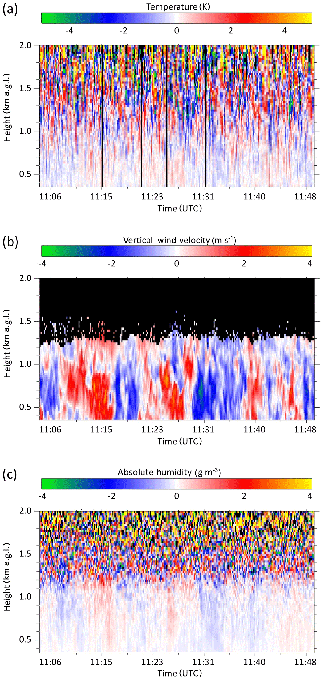
Figure 1 Time–height cross sections of the measurements of the detrended and despiked fluctuations of (a) temperature T^′, (b) vertical velocity w^′, and (c) absolute humidity q^′ measured with rotational Raman lidar, Doppler lidar, and water-vapor DIAL, respectively, on 24 April 2013 in the 45 min period between 11:05 and 11:50 UTC.

It is interesting to now compare the simultaneous fluctuations of temperature, humidity, and wind with each other. Updrafts ($w{}^{\prime }>\mathrm{0}$) are generally, but not always, related to warmer and moister air, while downdrafts ($w{}^{\prime }<\mathrm{0}$) are generally, but not always, cooler and dryer. This illustrates the CBL dynamics, which are mainly driven by buoyancy, but also their complexity.

The products of vertical wind fluctuations with temperature and with humidity fluctuations are shown in Fig. 2. Positive instantaneous latent heat flux values are dominant throughout the CBL, while the instantaneous sensible heat flux values are dominantly positive in the lower half of the CBL but negative in the upper half.

Figure 2 Time–height cross sections of the fluctuation products (a) $w{}^{\prime }T{}^{\prime }$, (b) $w{}^{\prime }q{}^{\prime }$, and (c) $T{}^{\prime }q{}^{\prime }$.

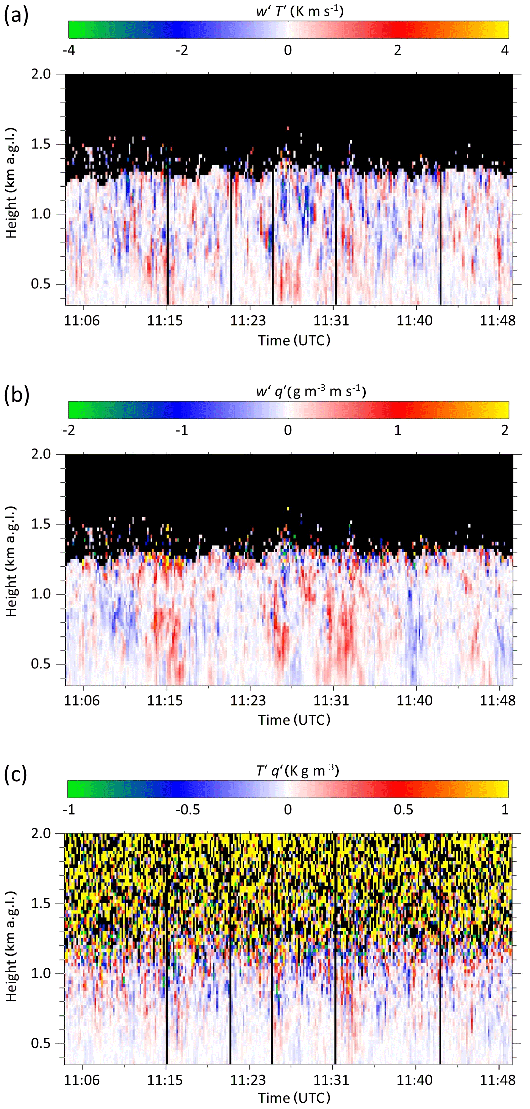
For completeness, Fig. 2 also shows the product of temperature and humidity fluctuations. Apart from noise, the data show partly positive and partly negative values. Positive values indicate that warmer air was moister, while cooler air was drier in the CBL. The fact that there are also negative data points reveals that cooler and moister as well as warmer and dryer fluctuations also appeared simultaneously here.

4.3 Integral scales and variances

For the variance data and noise uncertainties presented here, 20 data points of the structure function were used for the fit, giving a period of 200 s with 10 s resolution of the data. This is a reasonable number because the first zero crossing of the autocovariance function τ₀ is found at 2.5 times the integral scale (Behrendt et al., 2015; Wulfmeyer et al., 2016), which is mostly between 40 and 120 s in this case (see Fig. 3a). The integral scales were determined according to Eq. (42) of Wulfmeyer et al. (2016). We found that it is not a problem to use a few more lags (even beyond the zero crossing) in order to get a stable fit. The integral scale is a measure of the mean horizontal size of the eddies in the temporal domain during the measurement period (see, e.g., Lenschow et al., 2000, for details). Interestingly, this scale is usually different for different variables. In addition, by comparing the temporal resolution of the lidar measurements with the profile of the integral scale, we can make sure that the temporal resolution is high enough throughout the profile to resolve the major part of the turbulent fluctuations.

Figure 3 (a) Integral timescales of the atmospheric temperature fluctuations (RRL, red), atmospheric fluctuations of absolute humidity (WVDIAL, blue), and atmospheric fluctuations of the vertical wind (DL, green). The dashed line shows the mean CBL height determined with the RRL backscatter data at 1230 m a.g.l. Thin error bars in pale colors show the sampling uncertainties. (b) Same as (a) but for the variances. Thick error bars show the uncertainties due to instrumental noise.

The temperature variance profile in this case shows the typical peak near the CBL top (Fig. 3b). The value at z_i was ($\mathrm{0.46}\pm \mathrm{0.08}\pm \mathrm{0.13}$) K², with the first error for the sampling uncertainty and the second for the noise uncertainty. The humidity variance has a more complex structure here with a double peak near z_i (see also Muppa et al., 2016). The peak at 0.9 z_i was ($\mathrm{0.17}\pm \mathrm{0.04}\pm \mathrm{0.01}$) (g m⁻³)², while the upper peak at 1.1 z_i was ($\mathrm{0.58}\pm \mathrm{0.11}\pm \mathrm{0.10}$) (g m⁻³)². The vertical wind variance also shows a secondary peak at z_i in this case, while the maximum is found in the middle CBL, as is typical. The maximum vertical wind variance appeared at 0.6 z_i and was ($\mathrm{1.67}\pm \mathrm{0.40}\pm \mathrm{0.03}$) (m s⁻¹)².

4.4 Correlation coefficients, heat flux profiles, and tendencies

The correlation coefficients (Eq. 10) of the lidar data (Fig. 1) are shown in Fig. 4. Figure 5 shows the sensible heat flux profile H(z) derived with the data shown in Fig. 1 via Eq. (3) together with the latent heat flux profile L(z). While positive values are found for H(z) in the lower and middle CBL, negative values are found in the upper CBL as well as in the lower free troposphere. The upward sensible heat flux in the lower and middle CBL is related to upward energy flux from the surface into the CBL, while the negative values above show the downward energy flux into the CBL by entrainment. The sign of the correlation coefficient r of w^′ and T^′ is just the same as the sign of H at the same height. The values of r lie between −1 and 1 with the exception of two data points between 1000 and 1100 m. These outliers are due to the statistical uncertainty of the data since the temperature variance is close to zero here. r is larger than 0.5 from 400 to about 600 m with a decreasing tendency with height. The maximum H was ($\mathrm{182}\pm \mathrm{112}\pm \mathrm{32}$) W m⁻² and appears at 0.5 z_i, again with the first error for the sampling uncertainty and the second for the noise uncertainty. At about 0.7 z_i, H and r change signs to negative values above. We estimated the entrainment flux near z_i by averaging the measurements between 0.95 and 1.05 z_i and obtained a value of ($-\mathrm{62}\pm \mathrm{27}\pm \mathrm{42}$) W m⁻². At our lowest measurement points between 400 and 500 m (corresponding to 0.3 to 0.4 z_i) we found a mean sensible heat flux of ($\mathrm{156}\pm \mathrm{34}\pm \mathrm{8}$) W m⁻². Taking these representative values at the lower and upper parts of our measurement range in the CBL, we obtain −0.28 W m⁻³ for the vertical divergence of the sensible heat flux. This corresponds (Eq. 18) to a temperature tendency term of $\mathrm{2.3}\times {\mathrm{10}}^{-\mathrm{4}}$ K s⁻¹ or 0.83 K h⁻¹.

Figure 4 Profiles of the correlation coefficients of the lidar data.

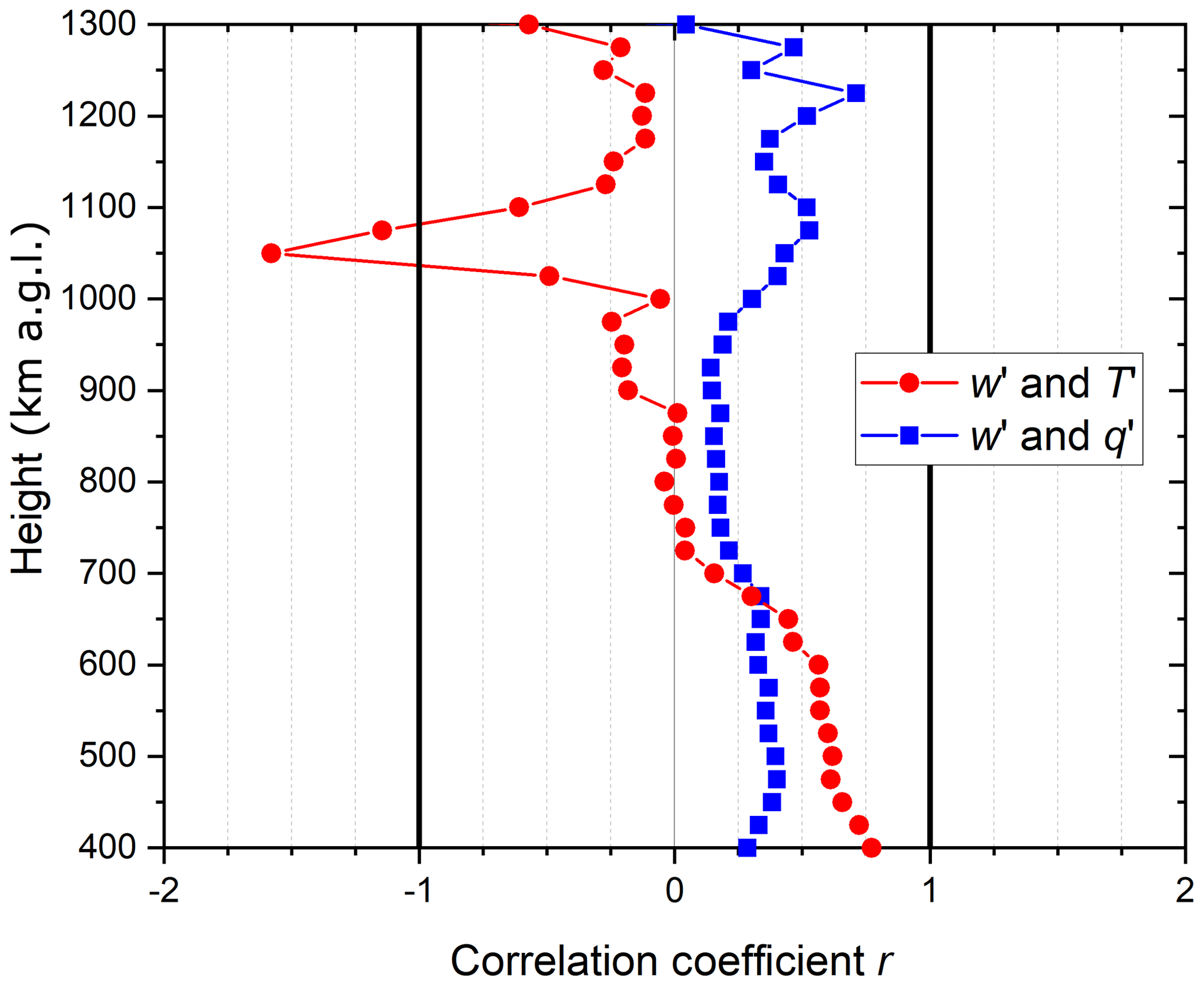
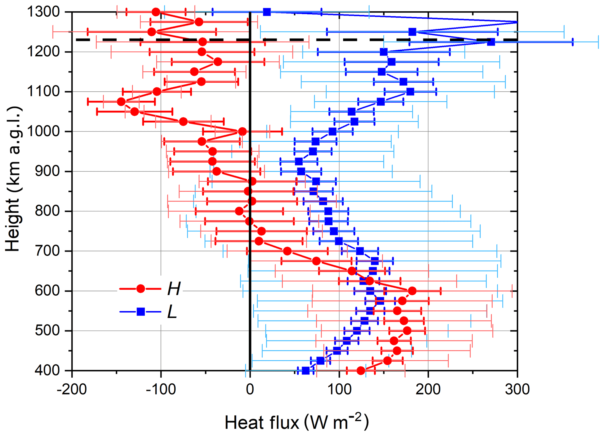
Figure 5 Sensible heat flux H and the latent heat flux L derived from the lidar data. The temperature and vertical wind fluctuations for determining H were obtained from UV rotational Raman lidar and coherent Doppler lidar measurements, respectively. For L, humidity fluctuations measured with a water-vapor DIAL were combined with vertical wind fluctuations measured with Doppler lidar. Thick error bars show the uncertainties due to instrumental noise; thin error bars in pale colors show the sampling uncertainties.

Figure 5 also shows the latent heat flux profile L(z) derived with the lidar data for comparison. The values are positive throughout the CBL as being typical. So are also the values of the correlation coefficients of moisture and vertical wind fluctuations (Fig. 4). This is because both upward moisture transport from the surface into the CBL and downward entrainment of dry air from the lower free troposphere into the CBL are related to positive values. Taking again representative values for the latent heat flux at the lower and upper parts of the boundary layer, we can determine the latent heat flux divergence and furthermore the water-vapor tendency (Wulfmeyer, 1999b). Between 400 and 500 m (corresponding to 0.3 to 0.4 z_i), we found a latent heat flux of ($\mathrm{95}\pm \mathrm{37}\pm \mathrm{5}$) W m⁻². The entrainment flux near z_i was ($\mathrm{190}\pm \mathrm{63}\pm \mathrm{39}$) W m⁻² (obtained again from 0.95 and 1.05 z_i. but with the outlier at 1275 m excluded). Over the range of the measurements, we thus get a latent heat flux divergence of 0.12 W m⁻³, which corresponds to a tendency of the absolute humidity due to the interplay of evapotranspiration and entrainment of $-\mathrm{5.3}\times {\mathrm{10}}^{-\mathrm{5}}$ (g m⁻³) s⁻¹ or −0.19 (g m⁻³) h⁻¹.

5 Summary and conclusions

We have presented the first measurements of sensible heat flux profiles H(z) in the daytime convective boundary layer made with ground-based remote sensing. The temperature fluctuations were obtained from UV rotational Raman lidar measurements, while the vertical wind measurements were made with a coherent Doppler lidar. A cloud-free 45 min analysis period of the HOPE campaign served as case study. The results show a typical profile of H(z) with positive values in the lower and middle CBL, namely, up to a value of ($\mathrm{182}\pm \mathrm{112}\pm \mathrm{32}$) W m⁻² found at 0.5 z_i, with the second and third number being the sampling uncertainty and noise uncertainty, respectively. In the upper CBL as well as in the lower free troposphere around z_i, we found negative values of H of about $(-\mathrm{62}\pm \mathrm{27}\pm \mathrm{42})$ W m⁻². With the profile of H(z), we obtained −0.28 W m⁻³ for the sensible heat flux divergence in the CBL, which corresponds to a warming tendency term of 0.83 K h⁻¹. Furthermore, we presented a simultaneously measured profile of the latent heat flux measured with a combination of the same Doppler lidar and a WVDIAL. The results showed an entrainment-drying CBL. Furthermore, the variance profiles of vertical wind as well as of the temperature and moisture fluctuations are shown. Given the feasibility of determining all these critical turbulent CBL variables together with lidar, we foresee that operating such instruments during field campaigns or even continuously in automated mode will provide very valuable data for model verifications and testing turbulence parameterizations because these flux profiles rule the distribution of humidity and temperature and thus the atmospheric stability and furthermore the formation of clouds and precipitation.