kCARTA: a fast pseudo line-by-line radiative transfer algorithm with analytic Jacobians, fluxes, nonlocal thermodynamic equilibrium, and scattering for the infrared

A fast pseudo-monochromatic radiative transfer package using a singular value decomposition (SVD) compressed atmospheric optical depth database has been developed, primarily for simulating radiances from hyperspectral sounding instruments (resolution ≥0.1 cm⁻¹). The package has been tested extensively for clear-sky radiative transfer cases, using field campaign data and satellite instrument data. The current database uses HITRAN 2016 line parameters and is primed for use in the spectral region spanning 605 to 2830 cm⁻¹. Optical depths for other spectral regions (15–605 and 2830–45 000 cm⁻¹) can also be generated for use by kCARTA. The clear-sky radiative transfer model computes the background thermal radiation quickly and accurately using a layer-varying diffusivity angle at each spectral point; it takes less than 30 s (on a 2.8 GHz core using four threads) to complete a radiance calculation spanning the infrared. The code can also compute non-local thermodynamic equilibrium effects for the 4 µm CO₂ region, as well as analytic temperature, gas and surface Jacobians. The package also includes flux and heating rate calculations and an interface to an infrared scattering model.

1 Introduction

Recent years have seen the launch and routine operation of new-generation infrared sounders on board Earth-orbiting satellites, for the purposes of providing measurements for data assimilation into numerical weather prediction (NWP) centers and for monitoring atmospheric composition. These hyperspectral instruments have low-noise channels with high resolution (≥0.5 cm⁻¹) and provide gigabytes of data daily, from about 620 to 2800 cm⁻¹. Examples include the Atmospheric Infrared Sounder (AIRS) (Aumann et al., 2003) on board NASA's Aqua satellite, the Infrared Atmospheric Sounding Interferometer (IASI) on board the Metop satellites (Clerbaux et al., 2009), and the Cross Track Infrared Sounder (CrIS) on board the Suomi and JPSS-1 satellites (Han et al., 2013).

The radiances measured by these instruments are obtained under all-sky conditions (i.e., clear or cloudy). Publicly available thermodynamic profiles retrieved from these voluminous data are presently performed after cloud-clearing the radiances (Susskind et al., 1998). Monochromatic line-by-line (MNLBL) codes are too slow for use in the operational retrievals from the cloud-cleared radiances. Instead, optical depths (or transmittances) produced by these MNLBL codes are parametrized for use in fast radiative transfer algorithms (RTAs), at the instrument resolution. The accuracy of the retrieved products depends on the accuracy of the fast models, which underlines the importance of the accuracy of line parameters and line shapes used in MNLBL codes, particularly the far-wing effects.

To satisfy the accuracy requirements of convolved optical depths and radiances used in developing and testing these fast models, the high-altitude (Doppler broadened) lines need to have monochromatic spectral resolutions of 0.0025 cm⁻¹ or better over the almost 2500 cm⁻¹ span of a typical infrared sounder. Using true MNLBL codes to produce optical depths for training the fast models is computationally intensive, as accurate line shapes needed to be computed for millions of spectral points, each at about 100 layers spanning a 0–80 km atmosphere, for about 40–50 gases; this has to be done for 50 or more profiles. The acceleration of this part of the process, needed to develop a fast RTA for the AIRS sounder, was the motivating factor behind the development of the work presented here. For this we also developed a line-by-line code (referred to as UMBC-LBL) to produce an accurate precomputed database of monochromatic atmospheric optical depths. Singular value decomposition (SVD) was then used to produce a highly compressed database (referred to as the kCompressed database; Strow et al., 1998) that is highly accurate, relatively small, and easy to use. When coupled to an accurate radiative transfer code, this pseudo-line-by-line package can be used as a starting point for developing tools for atmospheric retrievals (Rodgers, 2000). The key point to note is that though some optical depth information may be lost due to the compression and/or resolution of the database, the convolved radiances are very accurate.

To compute optical depths and radiances at any level for an arbitrary Earth atmospheric thermodynamic + gas profile, we paired together an uncompression algorithm for the kCompressed database with a one-dimensional clear-sky radiative transfer algorithm (RTA). The RTA works for both a down-looking and an up-looking instrument, with geometric ray tracing accounting for the spherical atmospheric layers. The generation of monochromatic transmittances from the compressed database is at least an order of magnitude faster than using a MNLBL code; for the long paths in the atmosphere the computed transmittances are smooth and well behaved and can be used to develop fast forward models. Radiances computed using the compressed database are as accurate as those computed with a MNLBL code as our compression procedure introduces errors well below spectroscopy errors (Strow et al., 1998).

The entire package is called kCARTA, which stands for “kCompressed Atmospheric Radiative Transfer Algorithm”. Although kCARTA is much slower than fast forward models which use effective convolved transmittances, it is much more accurate, and it can be used to generate optical depths and transmittances for developing the faster models. An example is the StandAlone Radiative Transfer Algorithm (SARTA) (Strow et al., 2003) for which kCARTA is the reference forward model; SARTA is used to retrieve level 2 geophysical products from the AIRS (Strow et al., 2003) and CrIS (Gambacorta, 2013) instruments. Other fast forward models for the infrared which parametrize the transmittances of the finite width instrument channels include a principal-component-based radiative transfer model (PCRTM; Liu et al., 2006), Radiative Transfer for TIROS Operational Vertical Sounder (RTTOV; Saunders et al., 1999), and the Jülich Rapid Spectral Simulation Code (JURASSIC; Hoffmann and Alexander, 2009).

kCARTA also includes algorithms to rapidly compute analytic Jacobians and is available in a Fortran 90 (f90) package. This package (v1.21, April 2019) uses some of the newer Fortran features such as implicit loops and function overloading and modules, and it includes code for computing fluxes, heating rates, and the effects of cloud and aerosol scattering using the Parametrization of Clouds for Longwave Scattering in Atmospheric Models (PCLSAM) (Chou et al., 1999) algorithm. While kCARTA was developed for use in the infrared region (605–2830 cm⁻¹), it is trivial to extend the database out in either direction, to span the far infrared to the ultra-violet. A clear-sky-only radiance + Jacobian MATLAB version is also available.

The speed and accuracy plus available run-time options of the code make it a very attractive alternative to other existing line-by-line codes. The literature is replete with papers and books describing spectroscopic calculations and monochromatic radiative transfer and flux calculations (see for example Goody and Yung, 1989; Edwards, 1992; Clough et al., 1992; Clough and Iacono, 1995; Tjemkes et al., 2002; Buehler et al., 2011; Schreier et al., 2014; Dudhia, 2017; Vincent and Dudhia, 2017), so here we chose to emphasize the features (and limitations) of kCARTA that would interest researchers working in these and related fields, and we apply kCARTA to quantify how different spectroscopic databases impact simulated clear-sky top-of-atmosphere (TOA) brightness temperatures. Focusing on the infrared (605–2830 cm⁻¹) region, this paper begins with a description of the line-by-line code and the kCompressed database, followed by a description of the clear-sky radiative transfer algorithm, together with Jacobians. The paper then discusses in detail some of the internal machinery of kCARTA, such as a background thermal computation developed for kCARTA, flux computations, and scattering packages.

2 Overview of line-by-line code and kCompressed database

2.1 UMBC-LBL

For an input set of (average temperature, pressure, and gas amount; in molecules per cubic centimeter) parameters, a custom monochromatic line-by-line code (UMBC-LBL) (De Souza-Machado et al., 2002) has been developed in order to accurately compute optical depths. This code defaults to the Van Vleck and Huber line shape (Van Vleck and Huber, 1977; Clough et al., 1980) for almost all molecules, using spectroscopic line parameters from the high-resolution transmission (HITRAN) molecular absorption database.

For each spectral region the UMBC-LBL optical depth computations are divided into bins that are typically 1 cm⁻¹ wide in the infrared. The optical depth in each of these bins is accumulated in three stages as shown in Fig. 1. (1) In the fine mesh stage absorption due to line centers within 1 cm⁻¹ of the bin edges is included at a very high resolution (typically 0.0005 cm⁻¹) and then integrated to the output (typically 0.0025 cm⁻¹) grid using a five-point boxcar; in Fig. 1 these are the red lines within the bin edges at ±0.5 cm⁻¹ and the blue lines within 1 cm⁻¹ of the same bin edges. (2) In the medium mesh stage absorption from line centers within 1–2 cm⁻¹ of the bin edges is included at 0.1 cm⁻¹ resolution, shown in green in the figure. (3) Finally, in the coarse mesh stage absorption from line centers within 2–25 cm⁻¹ of the bin edges are included at 0.5 cm⁻¹ resolution (none shown in the figure); for (2) and (3) the results are interpolated to the output grid. The black line is the accumulated optical depth for that bin.

We note three points here. First, the default kCARTA uses 0.0005 cm⁻¹ resolution between 605 and 880 cm⁻¹ and 0.0025 cm⁻¹ from 805 to 2830 cm⁻¹ (after the five-point boxcar). Section 7 demonstrates that convolved radiances computed with these resolutions compare very well against other RTAs, especially after convolving with a typical hyperspectral sounder response function. Second, the above line-by-line computations are very similar to those in other models (Edwards, 1992; Dudhia, 2017), but we use the “medium” bins and “coarse” bins for the lines whose centers are within the intervals lying within ± (1, 2) and ± (2, 25) cm⁻¹, respectively, of the bin edges, instead of using only coarse bins. Thirdly we note that for most Earth atmosphere molecules, the line strength–gas amount combination means the optical depth contribution due to line centers further than 25 cm⁻¹ away from the bin is negligible and can be ignored (Dudhia, 2017); the exception for the Earth atmosphere are H₂O and CO₂, which have countless strong lines further than 25 cm⁻¹ away from bin edges. To speed up the optical depth calculations, the weak but non-negligible contribution from these “far lines” is added in using a continuum optical depth contribution which depends on temperature and gas absorber amount.

Figure 1 Line-by-line calculations from UMBC-LBL. The bin of interest is at (−0.5, +0.5) cm⁻¹. Line shapes whose line centers are within this bin (red) and within ±1 cm⁻¹ of the bin edge (blue) are computed using high spectral resolution; line centers that are further out (green) have the line shapes computed at medium resolution and then interpolated to a higher resolution; line centers even further away (not shown) are computed at coarse resolution. The black curve is the sum over all the line contributions within that bin.

The above steps are followed for almost all molecules. Modifications to the above steps are needed for water vapor (which is separated into the traditional “basement” plus “continuum” contributions; Clough et al., 1980, 1989) and CO₂ in the 4 and 15 µm region, which needs line-mixing line shapes (Strow and Pine, 1988; Tobin et al., 1996; Niro et al., 2005; Lamouroux et al., 2015). Other molecules have optical depths that are more easily modeled with the Van Huber line shape, though recently the infrared absorption due to CH₄ has been modeled using line mixing (Tran et al., 2006). The UMBC-LBL optical depth computation for water vapor should be robust at all frequencies and allows the addition of water continuum models such as the recent MT CKD 3.2 coefficients (Mlawer et al., 2012). Spectra from UMBC-LBL have been extensively compared against optical depths computed by models such as the Line-by-Line Radiative Transfer Model (LBLRTM) (Clough et al., 1992, 2005) and the General line-by-line Atmospheric Transmittance and Radiance model (GENLN2) (Edwards, 1992).

2.2 kCompressed database

When applied toward any realistic Earth atmosphere simulation for an observing instrument, the UMBC-LBL calculations described above become impractically slow as they need to be performed for multiple gases in the atmosphere, over ∼100 atmospheric layers and encompassing a wide spectral range.

UMBC-LBL is therefore primarily used to generate an uncompressed database of lookup tables as described below. For each gas other than water vapor, the spectra are computed using the US Standard Atmosphere temperature profile, as well as five temperature offsets (in steps of 10 K) on either side of the temperature profile, for a total of 11 temperatures. Tests using NWP profiles show this is usually sufficient everywhere except for a handful of locations over the winter in Antarctica, which could fall slightly outside the coldest offset (on average by about 3 K) between 600 and 1000 mb; kCARTA handles these extreme cold cases by extrapolating what has been compressed and zero checking the optical depths.

The default infrared database spans 605–880 and 805–2830 cm⁻¹, broken up into 10 000 point intervals that are 5 and 25 cm⁻¹ wide, respectively. Each file contains matrices to compute optical depths for these 10 000 points at the set resolution. The 100 average pressure layers used in making the database are from the AIRS Fast Forward Model. The layers span from 1100 to 0.005 mb (about ground level to 85 km), and were chosen such that there is less than 0.1 K brightness temperature (BT) errors in the simulated AIRS radiances. The layers are about 200 m thick at the bottom of the atmosphere, gradually getting thicker with height (about 0.65 km at 10 km and 6 km at an altitude of 80 km).

These 10$\mathrm{000}\times \mathrm{100}\times \mathrm{11}$ optical depth intervals are then compressed using singular value decomposition (SVD) to produce the kCompressed database. Each compressed file will have a matrix of basis vectors B (size 10 000×N) and compressed optical depths D^′ (size $N\times \mathrm{100}\times \mathrm{11}$), where N is the number of significant singular vectors found. The prime denotes the compression worked more efficiently when the optical depths were scaled to the (1∕4)th power (Strow et al., 1998; Rodgers, 2000).

The self broadening of water is accounted for by generating monochromatic lookup tables for the reference water amount, multiplied by 0.1, 1.0, 3.3, 6.7, and 10.0 at the 11 temperature profiles specified above, meaning D^′ for water will have an extra dimension of length 5. Note that for the infrared we treat the HDO isotope (HITRAN isotope 4) as a separate gas from the rest of the water vapor isotopes.

The compressed optical depths D^′ vary smoothly in pressure, meaning the user is not limited to only using the 100 AIRS layers. For an arbitrary pressure layering, the lookup tables are uncompressed using spline or linear interpolation in temperature and pressure and scaled in gas absorber amount. Temperature interpolation of matrix D^′ for an AIRS 100-layer atmosphere therefore results in a matrix D^′′ of size N×100, and the final optical depths (of size 10 000×100) are computed using (BD^′′)⁴. Both the spline and linear interpolations allow easy computation of the analytic temperature derivatives, from which kCARTA can rapidly compute analytic Jacobians (see Sect. 5). The cumulative optical depth for each layer in the atmosphere is obtained by a weighted sum of the individual gas optical depths, with accuracy limited by that of the compressed database (Strow et al., 1998). The interested reader is referred to Vincent and Dudhia (2017) for a further discussion of other RTAs that use compressed databases.

The most recent kCompressed database uses line parameters from the HITRAN 2016 database (Rothman et al., 2013; Gordon et al., 2017), which together with the UMBC-LBL line shape models determine the accuracy of the spectral optical depths in this database. UMBC-LBL CO₂ line-mixing calculations use parameters that were derived a few years ago. Newer line-mixing models exist and we now use optical depths computed using LBLRTM v12.8 together with the line parameter database file based on HITRAN 2012 (aer_v_3.6) and (a) CO₂ line mixing by Lamouroux et al., 2010, 2015) and (b) CH₄ line mixing by (Tran et al., 2006).

In addition complete kCompressed databases for the IR using optical depths only from HITRAN 2012, LBLRTM v12.4 code, and GEISA 2015 (Husson et al., 2015) have been generated for comparison purposes. At compile time we usually point kCARTA to the HITRAN 2016 kCompressed database made by UMBC-LBL, but at the run time we have switches that easily allow us to swap in, for example, the CO₂ and CH₄ tables generated from LBLRTM.

The original lookup tables for the thermal infrared occupy hundreds of gigabytes, while the compressed monochromatic absorption coefficients are a much more manageable 824 megabytes (218 megabytes (water + HDO) + 76 megabytes (CO₂) + 530 megabytes (about 40 other molecular and 30 cross-section gases)). A general overview of some of the factors involved in compressing lookup tables for use in speeding up line-by-line codes is found in Vincent and Dudhia (2017), while more details about the detailed testing and generation of the kCARTA SVD compressed database are found in Strow et al. (1998). Appendix B discusses the extension of the database to span 15 to 44 000 cm⁻¹, though we note that kCARTA lacks built-in accurate scattering calculations in the shorter wavelengths. In order to resolve the narrow Doppler lines at the top of the atmosphere, the resolution δν of the spectral bands in Appendix B is adjusted according to $\mathit{\delta }\mathit{\nu }\sim {\mathit{\nu }}_{\mathrm{0}}\sqrt{(k_{\mathrm{b}}T/m)}/c$, where ν₀ is the band center, and T and m are the temperature and mass of the molecule, respectively, while k_b and c are Boltzmann's constant and speed of light.

The default kCARTA mode is to use the first 42 molecular gases in the HITRAN database, together with about 30 cross-section gases, for which we have reference profiles. If the user does not provide the profiles for any of these gases, kCARTA uses the US standard profile for that gas. The user can also choose to only use a selected number of specified gases. While running kCARTA, the user can then define different sets of mixed paths, where some of the gases are either turned off or the entire profile is multiplied by a constant number, which is very useful when for example we want to include only certain gases when we parametrize optical depths for SARTA.

3 kCARTA clear-sky radiative transfer algorithm

As a stream of radiation propagates through a layer, the change in diffuse beam intensity R(ν) in a plane-parallel medium is given by the standard Schwarzschild equation (Liou, 1980; Goody and Yung, 1989; Edwards, 1992):

$$\begin{array}{}\text{(1)}& \mathit{\mu }{\displaystyle \frac{\mathrm{d}R\left(\mathit{\nu }\right)}{\mathrm{d}{k}_{\mathrm{e}}}}=-R\left(\mathit{\nu }\right)+J\left(\mathit{\nu }\right),\end{array}$$

where μ is the cosine of the viewing angle, k_e is the extinction optical depth, ν is the wavenumber, and J(ν) is the source function. For a non-scattering clear sky, the source function is usually the Planck emission B(ν,T) at the layer temperature T, leading to an equation that can easily be solved for an individual layer. The general solution for a down-looking instrument measuring radiation propagating up through a clear-sky atmosphere can be written in terms of four components:

$$\begin{array}{}\text{(2)}& R\left(\mathit{\nu }\right)=R_{\mathrm{s}}\left(\mathit{\nu }\right)+R_{\text{lay}}\left(\mathit{\nu }\right)+R_{\mathrm{th}}\left(\mathit{\nu }\right)+R_{\text{solar}}\left(\mathit{\nu }\right),\end{array}$$

which are the surface, layer emissions, and downward thermal and solar terms, respectively. In terms of integrals the expressions can be written as (see e.g., Liou, 1980; Dudhia, 2017)

$$\begin{array}{}\text{(3)}& \begin{array}{rl}& R(\mathit{\nu },\mathit{\theta })={\mathit{ϵ}}_{\mathrm{s}}\left(\mathit{\nu }\right)B(\mathit{\nu },T_{\mathrm{s}}){\mathit{\tau }}_{\text{atm}}(\mathit{\nu },\mathit{\theta })\\ & +\underset{\text{surface}}{\overset{\text{TOA}}{\int }}B(\mathit{\nu },T(z\left)\right){\displaystyle \frac{\partial \mathit{\tau }(\mathit{\nu },\mathit{\theta })}{\partial s}}\mathrm{d}s+{\displaystyle \frac{\mathrm{1}-{\mathit{ϵ}}_{\mathrm{s}}\left(\mathit{\nu }\right)}{\mathit{\pi }}}{\mathit{\tau }}_{\text{atm}}\left(\mathit{\nu }\right)\\ & \int \mathrm{d}{\mathrm{\Omega }}^{+}\underset{\text{TOA}}{\overset{\text{surface}}{\int }}B(\mathit{\nu },T(s\left)\right){\displaystyle \frac{\partial \mathit{\tau }\left(\mathrm{\Omega }\right)}{\partial s}}\cos \left(\mathit{\theta }\right)\mathrm{d}s\\ & +{\mathit{\rho }}_{\mathrm{s}}\left(\mathit{\nu }\right)B_{⊡}\left(\mathit{\nu }\right)\cos \left({\mathit{\theta }}_{⊡}\right){\mathit{\tau }}_{\text{atm}}(\mathit{\nu },{\mathit{\theta }}_{⊡}){\mathit{\tau }}_{\text{atm}}(\mathit{\nu },\mathit{\theta })\end{array},\end{array}$$

where B(ν,T) is the Planck radiance at temperature T, T_s is the skin surface temperature, ϵ_s and ρ_s are the surface emissivity and reflectivity, B_⊡(ν) is the solar radiance at TOA, θ_⊡ is the solar zenith angle, θ is the satellite viewing angle, τ(ν,θ) is the transmission at angle θ, and τ_atm is the total atmospheric transmission. The dΩ⁺ in the middle term indicates integration over the upper hemisphere.

In what follows we discretize Eq. (2) so that layer i=1 is the bottom and i=N (=100) the uppermost layer, schematically shown in Fig. 2 for a clear-sky four-layer atmosphere, with O being the center of the Earth. A is the satellite while S is the satellite sub-point directly below it. Point P is the ground scene being observed by the satellite (slightly away from nadir), and N is the local normal at P. ∠SAP is the satellite scan angle while ∠APN is the satellite zenith angle θ; ∠NPI is the solar zenith angle θ_⊡. Note that as the radiation propagates through the pressure layers from P to H₁ to H₂ to H₃ to H₄ to A, the local angle (between the radiation ray and the local normal at any of the concentric circles) keeps changing due to the spherical geometry of the layers (refraction effects can also be included).

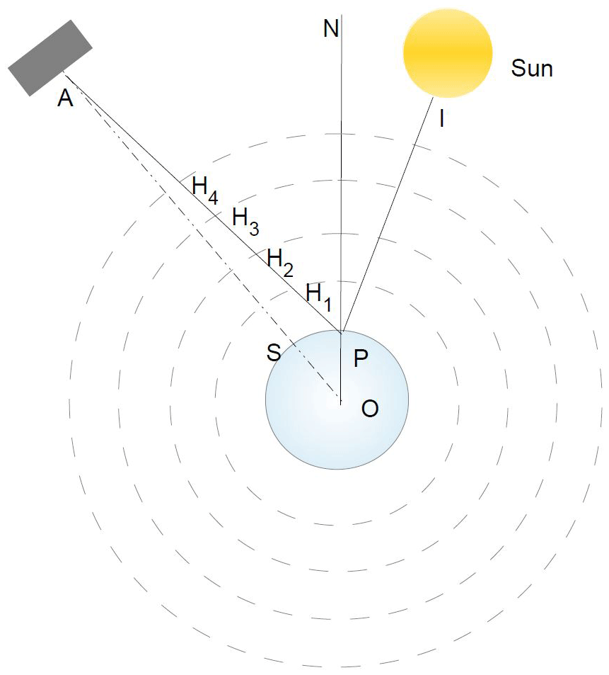
Figure 2 Viewing geometry for the sounders modeled by kCARTA. A is the satellite and point P is being observed by the satellite, while I is the sun.

The default mode of kCARTA (f90 version) assumes linear variation in layer temperature with optical depth, uses a background thermal diffusive angle that varies with the layer-to-ground optical depth (instead of a constant value typically assumed to be cos${}^{-\mathrm{1}}(\mathrm{3}/\mathrm{5})$), and performs ray tracing to account for the spherical atmospheric layers (but with no density effects). The f90 version of kCARTA also allows the user to choose constant layer temperature and to choose alternate ways of computing the background term, which will be discussed in Sect. 6.

Here we describe radiative transfer for the constant layer temperature case; see Sect. 6.2 for a short discussion when using the linear-in-tau option. For an arbitrary layer i with (nadir) optical depth k_i(ν), the transmittance of a beam passing from the bottom to the top of the layer at angle θ is given by ${\mathit{\tau }}_i(\mathit{\nu },\mathit{\theta })=e^{-k_i\left(\mathit{\nu }\right)/\cos \left(\mathit{\theta }\right)}$. The transmittance from the top of layer i to space is then the product of the individual transmittances of the layers above i

$$\begin{array}{}\text{(4)}& {\displaystyle }{\mathit{\tau }}_{i+\mathrm{1}\to \text{TOA}}(\mathit{\nu },\mathit{\theta })={\mathit{\pi }}_{j=i+\mathrm{1}}^N{\mathit{\tau }}_j(\mathit{\nu },\mathit{\theta }),\end{array}$$

with the special case of transmission from ground to space (i=0) involving all N layers.

The individual contributions to the upwelling radiance are then computed as follows.

3.1 Surface emission

The kCARTA surface emission is given by

$$\begin{array}{}\text{(5)}& R_{\mathrm{s}}\left(\mathit{\nu }\right)={\mathit{ϵ}}_{\mathrm{s}}\left(\mathit{\nu }\right)B(\mathit{\nu },T_{\mathrm{s}}){\mathit{\tau }}_{\text{GND}\to \text{TOA}}(\mathit{\nu },\mathit{\theta }),\end{array}$$

where ϵ(nu) is the user-supplied emissivity.

3.2 Layer emission

The atmospheric absorption and re-emission is modeled as

$$\begin{array}{}\text{(6)}& R_{\text{lay}}=\sum _{i=\mathrm{1}}^{i=N}B(\mathit{\nu },T_i)(\mathrm{1.0}-{\mathit{\tau }}_i(\mathit{\nu }\left)\right){\mathit{\tau }}_{i+\mathrm{1}\to \text{TOA}}(\mathit{\nu },\mathit{\theta }).\end{array}$$

Layers with negligible absorption (τ_i→1) contribute negligibly to the overall radiance, while those with large optical depths (τ_i→0) “black” out radiation from below. (1.0−τ_i(ν)) is the emissivity of the layer while $(\mathrm{1.0}-{\mathit{\tau }}_i(\mathit{\nu }\left)\right){\mathit{\tau }}_{i+\mathrm{1}\to \text{TOA}}(\mathit{\nu },\mathit{\theta })$ is the weighting function W_i of the layer.

3.3 Background thermal radiation

The atmosphere also emits radiation downward, at all angles, in a manner analogous to the upward layer emission just discussed. The total background thermal radiance at the surface is an integral over all (zenith and azimuth) radiance streams propagating from the top of the atmosphere (set to 2.7 K) to the surface. This is time consuming to compute using quadrature, and one approximation is to use a single effective (or diffusivity) angle of ${\mathit{\theta }}_{\text{diff}}={\cos }^{-\mathrm{1}}(\mathrm{3}/\mathrm{5})$ at all layers and wavenumbers:

$$\begin{array}{}\text{(7)}& \begin{array}{rl}& R_{\text{th}}^{\text{surface}}\left(\mathit{\nu }\right)=\mathit{\pi }{\mathit{\rho }}_{\mathrm{s}}\sum _{i=N}^{i=\mathrm{1}}B\left(T_i\right)\left[{\mathit{\tau }}_{i-\mathrm{1}\to \text{ground}}(\mathit{\nu },{\mathit{\theta }}_{\text{diff}})\right.\\ & -{\mathit{\tau }}_{i\to \text{ground}}(\mathit{\nu },{\mathit{\theta }}_{\text{diff}})\left.\right].\end{array}\end{array}$$

The summation is from the top of the atmosphere to the ground, and ρ_s is the surface reflectivity discussed above. Current sounders have channel radiance accuracy better than 0.2 K, so while the above term is much smaller than the surface or upwelling atmospheric emission contributions, it has to be computed accurately. Section 6 includes a detailed discussion of how kCARTA improves the accuracy of this background term by using a lookup table to rapidly compute a spectrally and layer-varying diffusive angle.

3.4 Solar radiation

Letting the surface reflectivity be denoted by ${\mathit{\rho }}_{\mathrm{s}}(\mathit{\nu },\mathit{\theta },\mathit{\varphi })$, then the solar contribution to the TOA radiance is given by

$$\begin{array}{}\text{(8)}& \begin{array}{rl}& R_{⊡}\left(\mathit{\nu }\right)={\mathit{\rho }}_{\mathrm{s}}(\mathit{\nu },\mathit{\theta },\mathit{\varphi })B_{⊡}\left(\mathit{\nu }\right)\cos \left({\mathit{\theta }}_{⊡}\right)\\ & \times {\mathit{\tau }}_{N\to \text{ground}}(\mathit{\nu },{\mathit{\theta }}_{⊡})\left){\mathit{\tau }}_{\text{ground}\to \text{TOA}}\right(\mathit{\nu },\mathit{\theta }\left)\right){\mathrm{\Omega }}_{⊡},\end{array}\end{array}$$

where B_⊡(ν) is the solar radiation at the top of the atmosphere and accounts for the solar disk. Over ocean, if the wind speed and solar and satellite azimuth angles are known, the reflectivity can be precomputed using the bidirectional reflectance distribution function (BRDF) and input to kCARTA; see for example Appendix C in Nalli et al., 2016. It is not easy to compute the BRDF over land, and the reflectivity could be simply modeled as ${\mathit{\rho }}_{\mathrm{s}}\left(\mathit{\nu }\right)=\frac{\mathrm{1}-{\mathit{ϵ}}_{\mathrm{s}}\left(\mathit{\nu }\right)}{\mathit{\pi }}$.

${\mathrm{\Omega }}_{⊡}=\mathit{\pi }(r_{\mathrm{s}}/d_{\mathrm{se}}{)}^{\mathrm{2}}$ is the solid angle subtended at the Earth by the sun, where r_e is the radius of the sun and d_se is the Earth–sun distance. The solar radiation incident at the TOA B_⊡(ν) comes from data files related to the ATMOS mission (Farmer et al., 1987; Farmer and Norton, 1989) and is modulated by the angle the sun makes with the vertical, cos (θ_⊡) (day-of-year effects are not included in the Earth–sun distance).

4 Nonlocal thermodynamic equilibrium computations

During the daytime, incident solar radiation is preferentially absorbed by some CO₂ and O₃ infrared bands, whose kinetic temperature then differs from the rest of the bands or molecules. This leads to enhanced emission by the lines in these bands.

Limb sounders detect NLTE effects in the 15 µm CO₂ bands (and in other molecular bands, for example O₃) due to the extremely long paths involved, but these are not modeled in the package as kCARTA is designed for nadir sounders.

For a nadir sounder, the most important effects are seen in the CO₂ 4 µm (ν₃) band. kCARTA includes a computationally intensive line-by-line nonlocal thermodynamic equilibrium (NLTE) model to calculate the effects for this CO₂ band. The model requires the kinetic temperature profile and NLTE vibrational temperatures of the strong bands in this region to compute the optical depths and Planck modifiers for the strong NLTE bands and the weaker LTE bands (Edwards et al., 1993, 1998; Lopez-Puertas and Taylor, 2001; Zorn et al., 2002), which are then used to compute a monochromatic top-of-atmosphere nadir radiance.

AIRS provided the first high-resolution nadir data of NLTE in the 4 µm CO₂ band. Using the kCARTA NLTE line-by-line model, a fast NLTE model (De Souza-Machado et al., 2007) for sounders has already been developed, which is used in the NASA AIRS L2 operational product.

5 Clear-sky Jacobian algorithm

Retrievals of atmospheric profiles (temperature, humidity, and trace gases) minimize the differences between observations and calculations, by adjusting the profiles using the linear derivatives (or Jacobians) of the radiance with respect to the atmospheric parameters. This section describes the computation of analytic Jacobians by kCARTA. Note that kCARTA currently computes Jacobians and weighting functions using a constant layer temperature assumption. For a downward-looking instrument, for simplicity consider only the upwelling terms in the radiance equation (atmospheric layer emission and the surface terms). Assuming a nadir satellite viewing angle, the solution to Eq. (1) is

$$\begin{array}{}\text{(9)}& \begin{array}{rl}& R\left(\mathit{\nu }\right)={\mathit{ϵ}}_{\mathrm{s}}B(T_{\mathrm{s}},\mathit{\nu }){\mathit{\tau }}_{\mathrm{1}\to \text{TOA}}\left(\mathit{\nu }\right)\\ & +{\mathrm{\Sigma }}_{i=\mathrm{1}}^{i=N}B(T_i,\mathit{\nu })(\mathrm{1.0}-{\mathit{\tau }}_i(\mathit{\nu }\left)\right){\mathit{\tau }}_{i+\mathrm{1}\to \text{TOA}}\left(\mathit{\nu }\right).\end{array}\end{array}$$

Differentiation with respect to the m-layer variable s_m (gas amount or layer temperature $s_m=q_{m\left(g\right)},T_m$) yields

$$\begin{array}{}\text{(10)}& \begin{array}{rl}& {\displaystyle \frac{\partial R\left(\mathit{\nu }\right)}{\partial s_m}}={\mathit{ϵ}}_{\mathrm{s}}B\left(T_{\mathrm{s}}\right){\displaystyle \frac{\partial {\mathit{\tau }}_{\mathrm{1}\to \text{TOA}}\left(\mathit{\nu }\right)}{\partial s_m}}\\ & +\sum _{i=\mathrm{1}}^{N}B(T_i,\mathit{\nu })(\mathrm{1.0}-{\mathit{\tau }}_i(\mathit{\nu }\left)\right){\displaystyle \frac{\partial {\mathit{\tau }}_{i+\mathrm{1}}\left(\mathit{\nu }\right)}{\partial s_m}}\\ & +\sum _{i=\mathrm{1}}^N{\mathit{\tau }}_{i+\mathrm{1}\to \text{TOA}}\left(\mathit{\nu }\right){\displaystyle \frac{\partial }{\partial s_m}}\left[B(T_i,\mathit{\nu })(\mathrm{1.0}-{\mathit{\tau }}_i(\mathit{\nu }\left)\right)\right],\end{array}\end{array}$$

where, as usual, ${\mathit{\tau }}_m\left(\mathit{\nu }\right)=e^{-k_m\left(\mathit{\nu }\right)}$ and ${\mathit{\tau }}_{m\to \text{TOA}}\left(\mathit{\nu }\right)={\mathrm{\Pi }}_{j=m}^N{e}^{-k_j\left(\mathit{\nu }\right)}$. The differentiation yields

$$\begin{array}{}\text{(11)}& \begin{array}{rl}& {\displaystyle \frac{\partial R\left(\mathit{\nu }\right)}{\partial s_m}}=\left[{\mathit{ϵ}}_{\mathrm{s}}B\left(T_{\mathrm{s}}\right){\mathit{\tau }}_{\mathrm{1}\to \text{TOA}}\right](-\mathrm{1}){\displaystyle \frac{\partial k_m\left(\mathit{\nu }\right)}{\partial s_m}}\\ & +\left[\sum _{i=\mathrm{1}}^{m-\mathrm{1}}(\mathrm{1.0}-{\mathit{\tau }}_i(\mathit{\nu }\left)\right)B_i\left(\mathit{\nu }\right)\mathit{\tau }(\mathit{\nu }{)}_{i+\mathrm{1}\to \text{TOA}}\right](-\mathrm{1}){\displaystyle \frac{\partial k_m\left(\mathit{\nu }\right)}{\partial s_m}}\\ & +\left[(\mathrm{1.0}-{\mathit{\tau }}_m(\mathit{\nu }\left)\right){\displaystyle \frac{\partial B_m\left(\mathit{\nu }\right)}{\partial s_m}}-B(T_m,\mathit{\nu }){\displaystyle \frac{\partial {\mathit{\tau }}_m\left(\mathit{\nu }\right)}{\partial s_m}}\right]\\ & {\mathit{\tau }}_{m+\mathrm{1}\to \text{TOA}}\left(\mathit{\nu }\right).\end{array}\end{array}$$

The individual Jacobian terms $\frac{\partial k_m}{\partial s_{m\left(g\right)}}$ are rapidly computed by kCARTA, as follows. The gas amount derivative is simply $\frac{\partial k_m}{\partial q_{m\left(g\right)}}=\frac{k_m}{q_{m\left(g\right)}}$ (with added complexity for water, to account for self-broadening), and the temperature derivative $\frac{\partial k_m}{\partial T}$ is cumulatively obtained while kCARTA is performing the temperature interpolations during the individual gas database uncompression.

The solar and background thermal contributions are also included in the Jacobian calculations. The thermal background Jacobians are computed at ${\cos }^{-\mathrm{1}}(\mathrm{3}/\mathrm{5})$ at all levels, for speed. This would lead to slight differences when comparing the Jacobians computed as above to those obtained using finite differences. kCARTA also computes the weighting functions and Jacobians with respect to the surface temperature and surface emissivity.

6 Background thermal and temperature variation in a layer

In this section we take a closer look at the computation of downwelling background thermal radiation and layer temperature variation.

6.1 Background thermal radiation

The contribution of downwelling background thermal to top-of-atmosphere upwelling radiances is negligible in regions that are blacked out as the instrument cannot see surface-leaving emissions. Similarly in layers/spectral regions where there is very little absorption and re-emission, the contribution is negligible as the effective layer emissivity (denoted by Δτ_i(ν) below) goes to zero. The background contribution thus needs to be performed most accurately in the window regions (low but finite optical depths); depending on the surface emissivity (and hence reflectivity) in the window regions, in terms of BT this term contributes as much as 4 K of the total radiance when reflected back up to the top of the atmosphere. The contribution at the surface by a downwelling radiance stream propagating at angle (θ,ϕ) through layer i is given by

$$\begin{array}{}\text{(12)}& \begin{array}{rl}& \mathrm{\Delta }{R}_i(\mathit{\nu },\mathit{\theta },\mathit{\varphi })\\ & =B(\mathit{\nu },T_i)(\mathrm{1.0}-{\mathit{\tau }}_i(\mathit{\nu },\mathit{\theta },\mathit{\varphi }\left)\right){\mathit{\tau }}_{i-\mathrm{1}\to \text{ground}}(\mathit{\nu },\mathit{\theta },\mathit{\varphi })\\ & =B(\mathit{\nu },T_i)\left({\mathit{\tau }}_{i-\mathrm{1}\to \text{ground}}\right(\mathit{\nu },\mathit{\theta },\mathit{\varphi })-{\mathit{\tau }}_{i\to \text{ground}}(\mathit{\nu },\mathit{\theta },\mathit{\varphi }\left)\right),\end{array}\end{array}$$

where θ is the zenith and ϕ is the azimuth angle, and τ_i→ground represents the layer-to-ground transmittances, derived from layer-to-ground optical depths x. This equation can be rewritten as

$$\begin{array}{}\text{(13)}& \mathrm{\Delta }{R}_i(\mathit{\nu },\mathit{\theta },\mathit{\varphi })=B(\mathit{\nu },T_i)\times \mathrm{\Delta }{\mathit{\tau }}_i(\mathit{\nu },\mathit{\theta },\mathit{\varphi }).\end{array}$$

An integral over (θ,ϕ) would give the contribution from the layer. The total downwelling spectral radiance at the surface would be a sum over all i layers (and the downwelling flux at the surface would be the integral over all wavenumbers).

The integral over the azimuth is straightforward (assuming isotropic radiation), but the integral over the zenith is more complex. Since the reflected background term is much smaller than the surface or atmospheric terms, a single stream at the effective angle ${\mathit{\theta }}_{\text{diff}}={\cos }^{-\mathrm{1}}(\mathrm{3}/\mathrm{5})$ (Liou, 1980) is often used as an approximation, at all layers and wavenumbers.

We have refined the computation as follows. Recall that ΔR(ν) in Eq. (13) depends on the layer-to-ground optical depth x, letting μ=cos θ the integral over the zenith (${\int }_{\mathrm{0}}^{\mathrm{1}}{e}^{-x/\mathit{\mu }}\mathit{\mu }d\mathit{\mu }=E_{\mathrm{3}}\left(x\right)$, more commonly known as the exponential integral of the third kind). The area under the E₃(x) curve would be the total flux coming from all optical depths ($\mathrm{0}\le x\le \mathrm{\infty }$); over 77 % of this area comes from the range $\mathrm{0}\le x\le \mathrm{1}$.

Applying the mean value theorem for integrals (MVTI) to E₃(x), we can write Eq. (13) in terms of two effective diffusive angles ${\mathit{\theta }}_{\mathrm{d}}^i,{\mathit{\theta }}_{\mathrm{d}}^{i-\mathrm{1}}$ at each layer i:

$$\begin{array}{}\text{(14)}& \begin{array}{rl}& \mathrm{\Delta }\mathit{\tau }(i,i-\mathrm{1})=\mathit{\tau }\left(i-\mathrm{1}\to \text{ground},{\mathit{\theta }}_{\mathrm{d}}^{i-\mathrm{1}},\mathit{\nu }\right)\\ & -\mathit{\tau }\left(i\to \text{ground},{\mathit{\theta }}_{\mathrm{d}}^i,\mathit{\nu }\right)R_{\text{th}}^{\text{surface}}\left(\mathit{\nu }\right)\\ & =\mathrm{2}\mathit{\pi }{\mathit{\rho }}_{\mathrm{s}}\sum _{i=N}^{i=\mathrm{1}}B(\mathit{\nu },T_i)\mathrm{\Delta }\mathit{\tau }(i,i-\mathrm{1})\end{array},\end{array}$$

with the effective angles varying as a function of the layer-to-ground space optical depth of that layer and the layer immediately below it. Numerical solutions to the MVTI show that when x→0 then μ_d→0.5 (or ${\mathit{\theta }}_{\mathrm{d}}\to \mathrm{60}{}^{\circ }$). Similarly, as x→∞ then ${\mathit{\theta }}_{\mathrm{d}}\to \mathrm{0}{}^{\circ }$, but this optically thick atmosphere means an instrument observing from the TOA cannot see the surface, so we use a lower limit (of 30^∘) for the diffusive angle. Finally when x=1.00 we find the special case ${\mathit{\mu }}_{\mathrm{d}}=\mathrm{0.59274}\simeq (\mathrm{3}/\mathrm{5})$. For “optically thin” regions, the layers closest to the ground contribute most to R_th(ν).

With today's high-speed computers, kCARTA uses an effective diffusive angle θ_d tabulated as a function of layer to ground optical depth x, as follows. For each 25 cm⁻¹ interval spanning the infrared range the layer L above which ${\cos }^{-\mathrm{1}}(\mathrm{3}/\mathrm{5})$ can be safely used was determined; below this layer, the lookup table is used. The table has higher resolution for x≤0.1 and becomes more coarse as x increases, with the effective diffusive angle cutoff at 30^∘ when the optical depths are larger than about 15.

We have tested this method of computing the background thermal against both the 20-point Gauss–Legendre quadrature and the three-point exponential Gauss quadrature (used by LBLRTM flux computations), and we found the method to be very accurate and fast, in terms of both the downwelling flux at the surface and also the final TOA computed radiance, even when the emissivity is as low as 0.8 (which means a significant contribution from the reflected thermal). At this low emissivity value, the constant ${\cos }^{-\mathrm{1}}(\mathrm{3}/\mathrm{5})$ diffusivity angle model produces a final TOA BT which differs from the Gauss–Legendre model by as much as 1.3 K (for the tropical profile) at for example 900 cm⁻¹, while the exponential quadrature and our model have errors smaller than 0.005 K.

6.2 Variation in layer temperature with optical depth

LBLRTM (Clough et al., 1992, 2005) has been extensively tested and shown to be very accurate in its computation of optical depths, radiances, and fluxes. In the computation of radiances, both kCARTA and LBLRTM codes use a “linear in τ” layer temperature variation; the former uses a higher-order expansion (accurate to O (τ⁵) for small τ) and also has an option to use “constant” layer temperature. Here we summarize the relevant equations. For an individual layer, with lower and upper boundary temperatures T_L and T_U, the linear in τ approximation leads to the following expression for the radiance at the top of the layer (rewritten from Eq. (13) in Clough et al., 1992):

$$\begin{array}{}\text{(15)}& \begin{array}{rl}& I\left(\mathit{\nu }\right)=I_{\mathrm{0}}\left(\mathit{\nu }\right)T+(\mathrm{1}-T)\mathit{\left\{}{B}_{\mathrm{av}}\right(\mathit{\nu })+(B_{\mathrm{u}}\left(\mathit{\nu }\right)-B_{\mathrm{av}}\left(\mathit{\nu }\right))\\ & \left(\mathrm{1}-\mathrm{2}\left({\displaystyle \frac{\mathrm{1}}{\mathit{\tau }}}-{\displaystyle \frac{T}{\mathrm{1}-T}}\right)\right)\mathit{\}},\end{array}\end{array}$$

where the optical depth τ includes the view angle $\mathit{\tau }={\mathit{\tau }}_{\text{layer}}/\cos \left(\mathit{\theta }\right)$ and transmission $T=\exp (-\mathit{\tau })$. I₀(ν) is the radiation incident at the bottom of the layer, B_av(ν) is the Planck radiance corresponding to the average layer temperature, while B_u(ν) is the Planck radiance corresponding to the upper boundary. For large τ, T→0 and I(ν)→B_u(ν). For small τ→0 the expression can be further expanded as follows:

$$\begin{array}{}\text{(16)}& \begin{array}{rl}& I\left(\mathit{\nu }\right)=I_{\mathrm{0}}\left(\mathit{\nu }\right)T+(\mathrm{1}-T)\mathit{\left\{}{B}_{\mathrm{av}}\right(\mathit{\nu })+(B_{\mathrm{u}}\left(\mathit{\nu }\right)-B_{\mathrm{av}}\left(\mathit{\nu }\right))\\ & \left({\displaystyle \frac{\mathit{\tau }}{\mathrm{6}}}-{\displaystyle \frac{{\mathit{\tau }}^{\mathrm{3}}}{\mathrm{360}}}+{\displaystyle \frac{{\mathit{\tau }}^{\mathrm{5}}}{\mathrm{15}\mathrm{120}}}\right)\mathit{\}}.\end{array}\end{array}$$

Comparing to the top of layer radiance in the constant in τ model,

$$\begin{array}{}\text{(17)}& I\left(\mathit{\nu }\right)=I_{\mathrm{0}}\left(\mathit{\nu }\right)T+(\mathrm{1}-T)B_{\mathrm{av}}\left(\mathit{\nu }\right),\end{array}$$

one sees the expressions are identical if there is no temperature variation, i.e., (B_u(ν)=B_av(ν)). The default kCARTA model layers are approximately 0.25 km thick (or a temperature spread of about 1.5 K for a 6 K km⁻¹ lapse rate) at the bottom of the atmosphere and about 2 km thick in the stratosphere (a temperature difference of 10 K). The gaseous absorption in these upper layers is typically negligible, except deep inside the strongly absorbing 15 and 4 µm CO₂ bands, which is where one would expect the largest differences between a linear-in-tau versus a constant-in-tau temperature model.

7 RTA intercomparisons: kCARTA versus LBLRTM

In this section we describe brightness temperature differences (ΔBT) between kCARTA and LBLRTM. As kCARTA is designed to be accurate for typical hyperspectral sounders, we show that after convolution the kCARTA spectral radiances compare very well against similarly convolved LBLRTM radiances; for completeness we also discuss how the monochromatic brightness temperature differences (ΔBT) change as a function of resolution in the 10–15 µm O₃ and temperature sounding regions.

For these runs we use our 49 regression profiles, with emissivity = 1 and reflectivity = 0 to exclude differences due to reflected thermal contributions. To exercise the kCARTA ray tracing, we use a ground satellite zenith angle of 24.5^∘, which becomes a TOA satellite scan angle of 22^∘ (typical average sounder scan angle). The tests are run at various kCARTA database resolutions. Note that when results are stated for a particular resolution, this means the kCARTA database (after five-point boxcar integration) was at this resolution; similarly the internal LBLRTM radiances were output at a resolution such that we can apply the same five-point boxcar for the radiance comparisons.

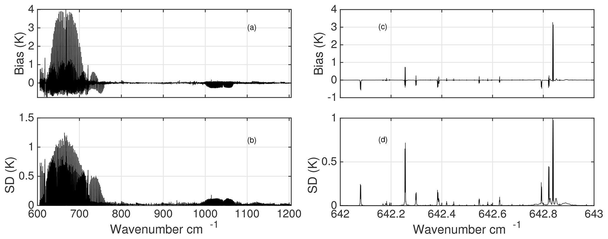
Figure 3 Panels (a–d) show the monochromatic BT differences (LBLRTM – kCARTA), with statistics obtained over 49 regression profiles, with the emissivity set to 1.0 and a 22^∘ satellite scan angle. Both sets of panels show the differences at 0.0005 cm⁻¹ resolution when only H₂O, CO₂, and O₃ optical depths from LBLRTM v12.8 are used. The largest differences are at the peaks of the high-altitude 15 µm CO₂ lines and decrease as the resolution is increased. Panels (c, d) are a zoom-in of (a, b), for a typical 15 µm region.

The comparisons are divided into two sets. For the first set of comparisons, we use an atmosphere consisting only of H₂O, CO₂, and O₃, with the optical depths generated using LBLRTM v12.8. This is done to assess the linear-in-tau radiative transfer while limiting differences due to spectroscopy, especially in the high-altitude 15 µm CO₂ and 10 µm O₃ sounding regions. For these tests, three resolutions spanning 605–1205 cm⁻¹ were used: 0.0025, 0.0005, and 0.0002 cm⁻¹.

At low resolution (0.0025 cm⁻¹), the mean differences right on top of the high-altitude temperature sounding lines in the 630–700 cm⁻¹ region are large (≥10 K). However, these differences drop significantly as we increase the resolution, to within 4 K ± 1.2 K at 0.0005 cm⁻¹ (default kCARTA resolution) and 1 K ± 0.4 K at 0.0002 cm⁻¹. The default kCARTA 0.0005 cm⁻¹ resolution results are shown in Fig. 3a, b. Panel (a) is the mean while the panel (b) is the standard deviation. Note that in the 10 µm O₃ sounding region (where the Doppler-broadened width of the high-altitude lines would be wider than in the 15 µm region), the differences are consistently much smaller: $-\mathrm{0.3}\pm \mathrm{0.1}$ K at 0.0005 cm⁻¹ resolution, dropping to $-\mathrm{0.1}\pm \mathrm{0.05}$ K at 0.0002 cm⁻¹ resolution.

Figure 3c, d show a zoom-in of a typical unit wavenumber interval deep in the 15 µm region and show the differences are zeros away from lines and largest around the peaks of the high sounding lines, each encompassing a very narrow spectral range of less than ∼0.005 cm⁻¹. These would be expected to contribute minimally to the convolutions using typical sounder spectral response functions, as will be shown below.

Taken together these mean that the kCARTA RTA is working as expected: in the very long wavelength 15 µm CO₂ region the differences decrease as we increase the spectral resolution while at 10 µm the differences remain quite small. We conjecture the remaining differences between kCARTA and LBLRTM are due to (a) algorithms: we use Eq. (16) to the 5th order while LBLRTM may use a Padé approximation and/or Eq. (16) to the 1st order; (b) there may be some very slight broadening effects right on top of the high-altitude CO₂ lines that we have not captured when generating the compressed database.

For the second set of monochromatic tests, kCARTA and LBLRTM used 42 molecular gases and 13 cross-section gases, using the current kCARTA default resolution of 0.0005 cm⁻¹ and 0.0025 cm⁻¹ for the spectral ranges 605–880 cm⁻¹ and 805–2830 cm⁻¹; the overlap region allows us to convolve the resulting radiances with AIRS spectral response functions (SRFs). Note that we used the default optical depths for kCARTA (currently HITRAN 2016, except for CO₂ and CH₄ which come from LBLRTM v12.8), while the LBLRTM v12.8 line file is based on HITRAN 2012. We only briefly summarize the monochromatic differences: deep in the 15 µm they are the same as Fig. 3a, b, but are noticeably different in other regions because of differences in underlying spectroscopy and (for high-altitude lines) possibly also resolution; for example on top of the 10 µm O₃ lines they could be as large as 5 K. Instead we show the differences after convolution with AIRS SRFs. Figure 4a, b show the biases and standard deviations of these differences; as described the noticeable differences at 10 and 6.7 µm arise primarily because of spectroscopy. For completeness, panels (c) and (d) show the mean BT spectra for the 49 regression panels (panels a and c) and the variation in computed BT (panels b and d), which are due to profile differences (temperature, H₂O, and O₃) as well as surface temperatures. Any user interested in reducing the monochromatic differences could easily do so by generating and using higher resolution compressed databases.

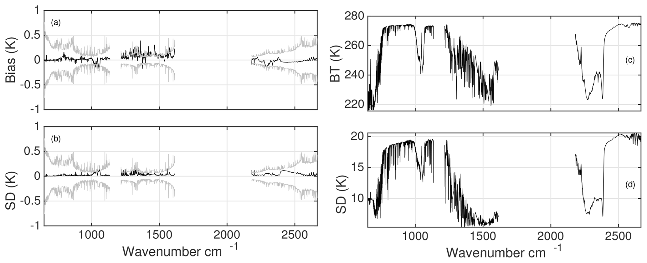
Figure 4 Results for 49 regression profiles, with 42 molecular gases and 13 cross-section gases, convolved using AIRS SRFs. The emissivity was set to 1.0 and a 22^∘ satellite scan angle. Panels (a, b) show the AIRS SRF convolved differences using the monochromatic differences (LBLRTM – kCARTA) seen in Fig. 3, but here with all gases added, and are due primarily to the different spectroscopy used by the two RTAs (except for the CO₂ and CH₄ gases); the grey curves are the AIRS NeDT at 250 K. Panels (c, d) show the mean calculated brightness temperature and standard deviation computed over 49 profiles. The variation in the 800–1200 cm⁻¹ region (and 2400–2680 cm⁻¹) is due to surface temperature differences and column water, while the variation in the other regions such as 10 and 7.6 µm is due to differing gas profiles of O₃ and H₂O; the variation in the 4 and 15 µm regions is due to temperature profile differences.

8 Flux computations

Longwave fluxes at the top and bottom of the atmosphere, as well as the heating and cooling rates, are computed by integrating spectral radiances from Eq. (2) over all angles and over the infrared spectral region: kCARTA is limited to the spectral range 15–3000 cm⁻¹ spanned by the different bands of kCARTA (see Appendix B). As in Sect. 7 the limitation of kCARTA for flux calculations is the spectral (infrared) resolution at every layer, compared to the varying-with-height resolution employed by other models such as LBLRTM. This impacts the high-altitude longwave cooling in the 15 µm CO₂ band. We use the Rapid Radiative Transfer (Longwave) model (RRTM-LW) (Mlawer et al., 2012) as our reference model for flux and heating rate comparisons in a clear-sky atmosphere. This fast model computes fluxes and heating rates in 16 bands spanning from 10 to 3000 cm⁻¹ and was developed using LBLRTM; the latter uses a varying spectral resolution at each layer (δν equal to four points per half-width in each layer), which means the spectra for the upper atmosphere layers have very high resolution. kCARTA uses the same approach as RRTM-LW and LBLRTM to compute fluxes and heating rates: the angular integration uses an exponential Gauss–Legendre with three or four terms, with a linear in τ layer temperature variation.

The accuracy of the flux and heating rate algorithm in kCARTA at the various resolutions was assessed by comparing fluxes and heating rates in the dominant 15 to 10 µm bands (fourth to eighth RRTM-LW bands, spanning 630–1180 cm⁻¹) computed using RRTM-LW and kCARTA, using the 49 regression profile set.

At 0.0025 cm⁻¹ resolution the kCARTA and RRTM-LW heating rates differ by less than 0.2 K d⁻¹ on average for altitudes below 40 km, but at higher altitudes the differences were much larger and could be 1.5 K d⁻¹. Switching to the 605–1205 cm⁻¹ H₂O, CO₂, and O₃ test atmosphere database at 0.0005 cm⁻¹ significantly improves the results, with heating rate differences dropping to about 0.2 K d⁻¹ almost everywhere.

Figure 5 shows the heating rate differences between kCARTA and RRTM-LW. Panel (a) shows differences between kCARTA and RRTM-LW, with the mean and standard deviation being solid and dashed, respectively; panel (b) shows mean calculations as a function of height. The blue curves were calculated at 0.0025 cm⁻¹ resolution while the red curves were calculated at higher than 0.0005 cm⁻¹ resolution. While the agreement is better than 0.05 K d⁻¹ in the lowest 30 km, Fig. 5 shows the heating rates using the low resolution begin to differ noticeably above 45 km (blue curve); conversely the high-resolution heating rates (red curves) are within 0.2 K d⁻¹ till about 65 km.

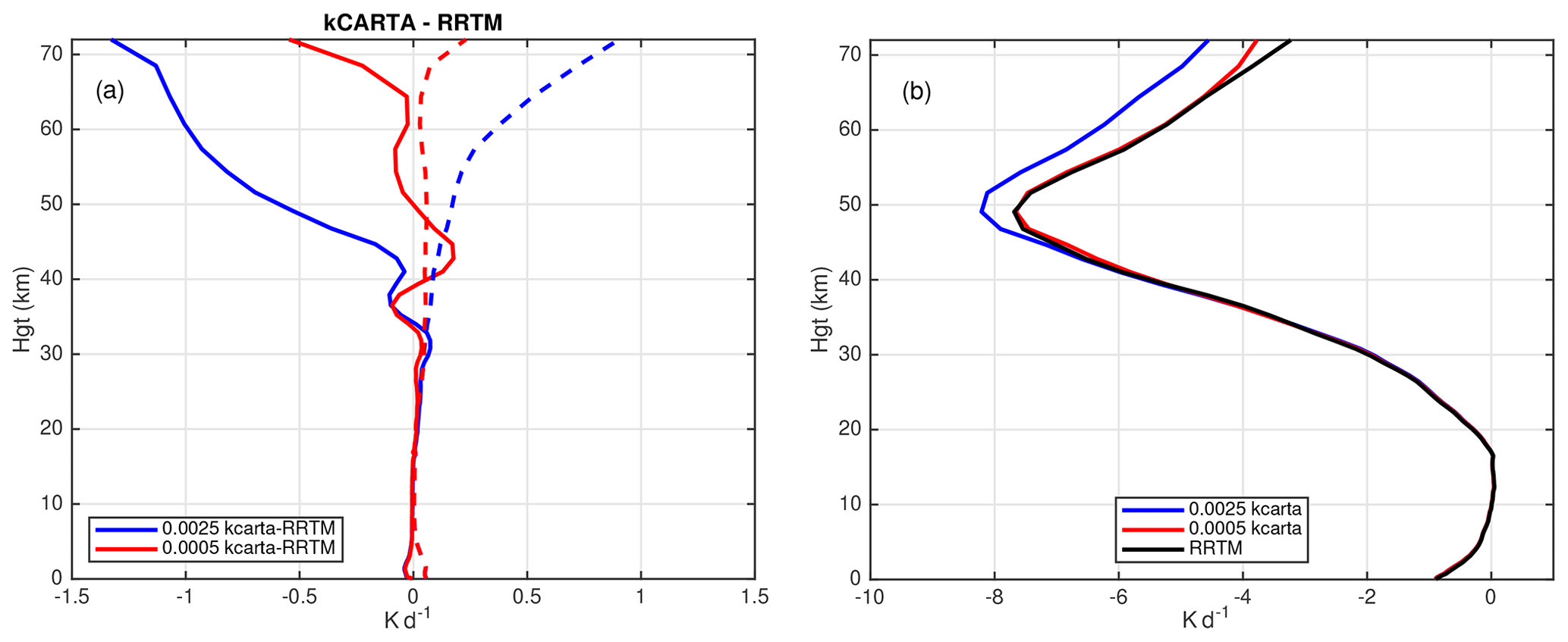
Figure 5 Heating rates for the 630–1180 cm⁻¹ region computed using low-resolution (0.0025 cm⁻¹; blue curves) and high-resolution (0.0005 cm⁻¹; red curves) kCARTA databases for 49 Earth-spanning atmosphere profiles, compared to RRTM-LW. Panel (a) shows differences in the heating rates, while (b) shows the mean heating rates.

9 Scattering package included with kCARTA Fortran 90 version

The daily coverage of hyperspectral sounders provides us with information pertaining to the effects of cloud contamination on measured radiances. Ignoring these effects can negatively impact retrievals used for weather forecasting and climate modeling. A scattering package based on the PCLSAM (Parametrization of Cloud Longwave Scattering for use in Atmospheric Models) scheme (Chou et al., 1999) has been interfaced into the f90 version of kCARTA (see Appendix C). The implementation allows kCARTA to compute radiances very quickly in the presence of scattering media such as clouds or aerosol. For a given scattering species and assumed particle shape and distribution, the extinction coefficients, single-scattering albedo, and asymmetry parameters needed by the scattering code are stored in tables as a function of wavenumber and effective particle size (for a particle amount of 1 g m⁻²). The PCLSAM package is optimized for use in the thermal infrared, away from regions where solar contributions are important. As kCARTA currently does not handle Rayleigh scattering, one can easily use kCARTA to output monochromatic optical depths that can be imported into well-known scattering packages. More details about PCLSAM and our cloud representation models are found in Appendix C.

10 Conclusions

We have described the details of a very fast and accurate pseudo-monochromatic code, optimized for the thermal infrared spectral region used by operational weather sounders for thermodynamic retrievals. It is much faster than line-by-line codes, and the accuracy of its spectroscopic database has been extensively compared to GENLN2 and more recently to LBLRTM. Updating the spectroscopy in a selected wavenumber region for a specified gas is as simple as updating the relevant file(s) in the database: for example, our custom UMBC-LBL enables us to rebuild entire databases within weeks of the latest HITRAN release.

The computed clear-sky radiances includes a fast, accurate estimate of the background thermal radiation. Analytic temperature and gas amount Jacobians can be rapidly computed. Early in the AIRS mission, comparisons of AIRS observations against kCARTA simulations allowed for the quick implementation of modifications to gas optical depths: our modifications to the CKD2.4 and MT-CKD 1.0 continuum versions are very similar to what is now in the MT-CKD2.5 version. We now use the MT-CKD 3.2 continuum, together with the N₂ and O₂ continuum contributions bundled with that same version. We use two resolutions in the infrared: 0.0005 cm⁻¹ for the 605–880 cm⁻¹ region (to accurately resolve the high-altitude CO₂ lines) and 0.0025 cm⁻¹ elsewhere; a user can easily switch to an alternate resolution by generating the appropriate compressed databases for use with kCARTA, though this could be at the expense of speed (at these current resolutions kCARTA takes 30 s to compute TOA spectra from 605 to 2830 cm⁻¹ while LBLRTM takes over 3 min). Tests show that brightness temperature differences between kCARTA and for example LBLRTM are largest right on top of a small number of high-altitude temperature sounding lines in the 15 µm region (and close to zero elsewhere); these differences decrease as the resolution is increased. Since the disparity is right at the peaks of the lines, the differences after convolution with a typical sounder SRF such as AIRS are on average much smaller than the NeDT.

kCARTA is fast enough to be used in optimal estimation retrievals for instruments spanning a reasonably small wavenumber range. The kCARTA database has been extended to include 15–44 000 cm⁻¹, which eventually needs to be updated to HITRAN 2016 (see the Appendix). In the future we plan to augment the optical depth calculations performed by UMBC-LBL by using speed-dependent line shapes as parameters become available.

Appendix A: UMBC-LBL and kCARTA downloads and auxiliary requirements

The kCompressed database is supplied in Fortran little-endian binary files that contain the optical depths for a specific gas. Each file contains optical depths at 10 000 spectral points and average pressures corresponding to the 100 AIRS layers. Links to the (605–2830 cm⁻¹) compressed database can be found at http://asl.umbc.edu/pub/packages/kCompressedDatabase.html (last access: 2 January 2020).

We also supply the US Standard Profile for all gases in the database and kLAYERS, a program that takes in a point profile (from sondes and NWPs) and outputs an AIRS 100-layer path-averaged profile (molecules cm⁻²). kLAYERS needs our supplied HDF file implementation (RTP) source code.

The MATLAB version should work with R2012+ while the compiler for the Fortran version must support structures, such as Absoft, ifort, and PGF. As the RTP file contains the atmospheric profile and scan geometry, both the MATLAB and f90 kCARTA only need a simple additional (name list) file to drive either code. The f90 version of kCARTA outputs binary files, which typically have header information such as kCARTA version number, number of layers and gases, and parameter setting values, followed by panels, each 10 000 points long, containing the optical depths, radiances, Jacobians or fluxes computed, and output by kCARTA. A number of MATLAB-based readers can then be used to further process the kCARTA output as needed. More information is found at http://asl.umbc.edu/pub/packages/ kcarta.html (last access: 12 January 2020).

A new compressed database (spanning the infrared 500–2830 cm⁻¹ region) is generated for kCARTA every 4 years, roughly within a few months of a HITRAN database release. The current f90 version described in this paper is identified on GitHub as SRCv1.21_f90 and currently uses HITRAN 2016 line parameters for all gases except CO₂ and CH₄ where we used LBLRTM v12.8 optical depths, together with the MT-CKD3.2 continuum. These were used to generate the most recent SARTA v2.01 fast model coefficients; earlier SARTA versions were developed using kCARTA v1.07 and v1.18 (with HITRAN databases updated as they became available).

Appendix B: Available spectral regions and f90 kCARTA features

Table B1 Spectral bands for kCARTA.

Asterisks indicate the region spanned by hyperspectral sounders, which kCARTA focuses on for testing and validation.

Table B2 kCARTA features.

^∗ Indicates currently only available in the f90 version.

The UMBC-LBL line-by-line code has been used to generate optical depths in the spectral regions seen in Table B1. The asterisks mark the 605–2830 cm⁻¹ spectral region spanned by the current hyperspectral sounders, where we focus our validation of spectroscopy and radiative transfer. The current database in this spectral region uses line shape parameters from HITRAN 2016. The Van Vleck and Huber line shape is used for all HITRAN molecules from ozone onward; water vapor uses the “without basement” plus MT-CKD 3.2, and CO₂, and CH₄ use line-mixing optical depths generated from LBLRTM v12.8. Note that in the important 4.3 µm temperature sounding region, the f90 version can also include the N₂∕H₂O and N₂∕CO₂ collision-induced absorption (CIA) effects modeled in Hartmann et al. (2018) and Tran et al. (2018), which depend on CO₂, H₂O, and N₂ absorber amounts.

A clear-sky radiance calculation in the infrared takes about 30 s, using a 2.8 GHz 32-core multi-threading Intel machine. The run time goes to 120 s if Jacobians are also computed (for nine gases). A full radiance calculation from 15 to 44 000 cm⁻¹ takes less than 5 min.

Table B2 lists a number of the features of kCARTA, with the ones marked by an asterisk only available in the f90 version. Note that the tables default to describing the spectroscopy for the infrared region.

The spline versus linear temperature interpolation differences, as tested on 49 regression profiles, are 0.0004±0.0040 K, with a maximum absolute difference of 0.342 K (in the 15 µm region).

Appendix C: PCLSAM scattering algorithm

The PCLSAM scattering algorithm for longwave radiances has applications ranging from dust retrievals (De Souza-Machado et al., 2010) to modeling the effects of clouds on sounder data (Matricardi, 2005; Vidot et al., 2015). This scattering model changes the extinction optical depth from k(ν) to a parametrized number $k_{\text{eff. extinction}}^{\text{scatterer}}\left(\mathit{\nu }\right)$ (Chou et al., 1999) and is designed for cases of the single-scattering albedo ω being much less than 1, such as in the thermal infrared, where ω for cirrus and water droplets and aerosols is typically on the order of 0.5.

Since $k_{\text{eff. extinction}}^{\text{scatterer}}\left(\mathit{\nu }\right)$ is now effectively the absorption due to the cloud or aerosol, for each layer i that contains scatterers we replace the gas absorption optical depth with the total absorption optical depth:

$$\begin{array}{}\text{(C1)}& k_{\text{total}}\left(\mathit{\nu }\right)=k_{\text{atm}}^{\text{gases}}\left(\mathit{\nu }\right)+k_{\text{eff. extinction}}^{\text{scatterer}}\left(\mathit{\nu }\right),\end{array}$$

where (Chou et al., 1999) $k_{\text{eff. extinction}}^{\text{scatterer}}\left(\mathit{\nu }\right)=k_{\text{extinction}}^{\text{scatterer}}\left(\mathit{\nu }\right)\times (\mathrm{1}-\mathit{\omega }(\mathit{\nu }\left)\right)(\mathrm{1}-b(\mathit{\nu }\left)\right)$ and the backscatter $b\left(\mathit{\nu }\right)=(\mathrm{1}-g(\mathit{\nu }\left)\right)/\mathrm{2}$, with g(ν) being the asymmetry factor. Using this for every layer containing scatterers, the radiative transfer algorithm is now the same as clear-sky radiative transfer, with very little speed penalty.

kCARTA is capable of using a TwoSlab (De Souza-Machado et al., 2018) cloud representation scheme for use with PCLSAM. This allows for non-unity fractions for up to two clouds, so that radiative transfer then assumes the total radiance is a sum of four radiance streams (clear, cloud 1, cloud 2, and the cloud overlap) weighted appropriately:

$$\begin{array}{}\text{(C2)}& r\left(\mathit{\nu }\right)=c_{\text{overlap}}{r}^{\left(\mathrm{12}\right)}\left(\mathit{\nu }\right)+c_{\mathrm{1}}{r}^{\left(\mathrm{1}\right)}\left(\mathit{\nu }\right)+c_{\mathrm{2}}{r}^{\left(\mathrm{2}\right)}\left(\mathit{\nu }\right)+f_{\text{clr}}{r}^{\text{clr}}\left(\mathit{\nu }\right).\end{array}$$

With this model kCARTA allows the user to specify up to two types of scatterers in the atmosphere (ice–water, ice–dust, and water–dust or even ice–ice, water–water, and dust–dust); the two scatterers are placed in separate “slabs” which occupy complete AIRS layers and are specified by cloud top/bottom pressure (millibars), cloud amount (g m⁻²), cloud effective particle diameter (µm). After the computations are done, all five radiances are output when two clouds are defined (overlap, two clouds separately, clear, and the weighted sum), and three radiances if only one cloud is defined (one cloud, clear, weighted sum).

Analytic Jacobians for temperature, gas amounts, and cloud microphysical parameters (effective size and loading) can also be computed, as can be fluxes and associated heating rates, though the slab boundaries could introduce spikes in the heating rate profiles.

kCARTA does not have built-in multiple-scattering capabilities to handle, for example, Rayleigh scattering in the ultra-violet. To handle this we have written MATLAB routines to read in kCARTA optical depths and pipe them into LBLDIS (Turner et al., 2003; Turner, 2005), a code that merges optical depths and scattering using the extensively tested discrete ordinate radiative transfer (DISORT) (Stamnes et al., 1988) algorithm.