Can statistics of turbulent tracer dispersion be inferred from camera observations of SO₂ in the ultraviolet? A modelling study

Atmospheric turbulence and in particular its effect on tracer dispersion may be measured by cameras sensitive to the absorption of ultraviolet (UV) sunlight by sulfur dioxide (SO₂), a gas that can be considered a passive tracer over short transport distances. We present a method to simulate UV camera measurements of SO₂ with a 3D Monte Carlo radiative transfer model which takes input from a large eddy simulation (LES) of a SO₂ plume released from a point source. From the simulated images the apparent absorbance and various plume density statistics (centre-line position, meandering, absolute and relative dispersion, and skewness) were calculated. These were compared with corresponding quantities obtained directly from the LES. Mean differences of centre-line position, absolute and relative dispersions, and skewness between the simulated images and the LES were generally found to be smaller than or about the voxel resolution of the LES. Furthermore, sensitivity studies were made to quantify how changes in solar azimuth and zenith angles, aerosol loading (background and in plume), and surface albedo impact the UV camera image plume statistics. Changing the values of these parameters within realistic limits has negligible effects on the centre-line position, meandering, absolute and relative dispersions, and skewness of the SO₂ plume. Thus, we demonstrate that UV camera images of SO₂ plumes may be used to derive plume statistics of relevance for the study of atmospheric turbulent dispersion.

1 Introduction

Air motion in the lowest part of the atmosphere is bounded over land by a solid surface of varying temperature and roughness. This part of the atmosphere is named the planetary boundary layer (PBL; Stull, 1988). It responds quickly to surface radiation changes, and the air motion in the PBL is nearly always turbulent. A substance released into this turbulent atmosphere will, at locations downwind of its source, experience concentration fluctuations that are important, particularly if responses are non-linear, for example, with respect to toxicity, flammability and odour detection (e.g. Hilderman et al., 1999; Schauberger et al., 2012; Gant and Kelsey, 2012), and non-linear chemical reactions (Brown and Bilger, 1996; Vilà-Guerau de Arellano et al., 2004; Cassiani et al., 2013). The Camera Observation and Modelling of 4D Tracer Dispersion in the Atmosphere (COMTESSA) project (https://comtessa-turbulence.net/, last access: 16 June 2020) aims to “elevate the theory and simulation of turbulent tracer dispersion in the atmosphere to a new level by performing completely novel high-resolution 4D measurements”. Over short transport distances, sulfur dioxide (SO₂) may be considered to be a passive tracer. Furthermore, SO₂ strongly absorbs radiation in part of the UV spectrum and may thus be detected by, for example, UV-sensitive cameras (see, for example, Kern et al., 2010b, and references therein). Within COMTESSA, six UV cameras have been built to measure SO₂ densities from various viewing directions. A series of experiments with puff and continuous releases of SO₂ from a tower have been performed as described by Dinger et al. (2018). It is known from measurements of volcanic SO₂ emissions that aerosol and viewing geometry affect the retrieved SO₂ amounts (Kern et al., 2013). Furthermore, variations in surface albedo and solar zenith and azimuth angles may have an impact. The influence of these factors on the UV camera images, the deduced SO₂ amounts, and density statistics needs to be quantified and, if necessary, corrected for.

Kern et al. (2013) performed radiative transfer simulations, including a circular SO₂ plume, to estimate the effect of plume distance, SO₂ amount, and aerosol on the radiance at a UV camera location. However, to the authors' knowledge, UV camera images have not been simulated before. We present a novel method to simulate UV camera images of a dispersing SO₂ plume using a 3D radiative transfer model. The 3D description of the SO₂ plume is provided by large eddy simulation (LES) and is used in lieu of real atmospheric flow. The simulated images are used to examine how various factors (solar angles, aerosol content, and surface albedo) affect the statistical parameters characterizing the SO₂ plume dispersion. The LES providing the input to the radiative transfer modelling, the radiative transfer model used to simulate the camera images, and the statistical parameters are described in Sect. 2. The effects of solar azimuth and zenith angles, surface albedo, background aerosol, and aerosols in the plume on plume density statistics are presented in Sect. 3. Furthermore, the plume density statistics from the simulated images are compared with statistics derived directly from the LES simulations. The paper ends with the conclusions in Sect. 4.

2 Methods

2.1 Large eddy simulation (LES)

Large eddy simulation is nowadays viewed as a popular tool in many applied atmospheric dispersion studies, especially of the urban environment and for critical applications such as the release of toxic gas substances (e.g. Fossum et al., 2012; Lateb et al., 2016). LES provides access to the 3D turbulent flow field, and it is sometimes used as a replacement for experimental measurements at high Reynolds numbers. In this methodology, the large scales of the turbulent flow are explicitly simulated while a low-pass filter is applied to the governing equations to remove the small scales information from the numerical solution. The effects of the small scales are then parameterized by means of a sub-grid scale (SGS) model (e.g. Deardorff, 1973; Moeng, 1984; Pope, 2000; Celik et al., 2009). We used the Parallelized Large-Eddy Simulation Model (PALM; Raasch and Schröter, 2001; Maronga et al., 2015) to solve the filtered, incompressible Navier–Stokes equations in Boussinesq-approximated form at an infinite Reynolds number. A 3D domain of $\mathrm{1000}\mathrm{m}\times \mathrm{375}\mathrm{m}\times \mathrm{250}\mathrm{m}$ in the along wind (x), crosswind (y), and vertical (z) directions, respectively, was simulated with a grid resolution of $nx\times ny\times nz=\mathrm{1024}\times \mathrm{384}\times \mathrm{256}$. Here $nx,ny,$ and nz are the number of grid nodes in along wind, crosswind, and vertical directions, respectively. This implies that the size of a grid cell is 0.98³  m³≈1 m³. The release point was located at 25 and 150 m above the ground, depending on camera view direction; see Sect. 2.2.

The neutral boundary layer was simulated as an incompressible half-channel flow at an infinite Reynolds number. The flow was driven by a constant pressure gradient. For the velocity, periodic boundary conditions were used on the lateral boundaries while on the top a strictly symmetric, stress-free condition was applied. The bottom wall was not explicitly resolved, but a constant flux layer was used as is commonly done in atmospheric simulations. Non-periodic boundary conditions were set for the passive scalar. For further information on the model set-up, see also Ardeshiri et al. (2020).

The LES calculates 3D SO₂ concentrations as a function of time. The SO₂ concentrations are used as input to the 3D radiative transfer model simulations. A total of 100 time frames were calculated with a time resolution of 6.25 s. For the sensitivity studies one randomly chosen time frame was used, while seven and nine randomly chosen frames were used for the reference case calculation (see Sect. 3). Both parts of the plume close to the release point and further downstream were used as input for the camera simulations. In Fig. 1 examples are provided of the part of the plume viewed by the different cameras (see Sect. 2.2 for camera definition). Figure 1a and b show the SO₂ column densities along the y and z axes, respectively, for one instant of the LES simulation. Figure 1a shows approximately the part of the plume seen by camera A. Figure 1c, d, and e show the part of the plume viewed by cameras B, C, and D, respectively.

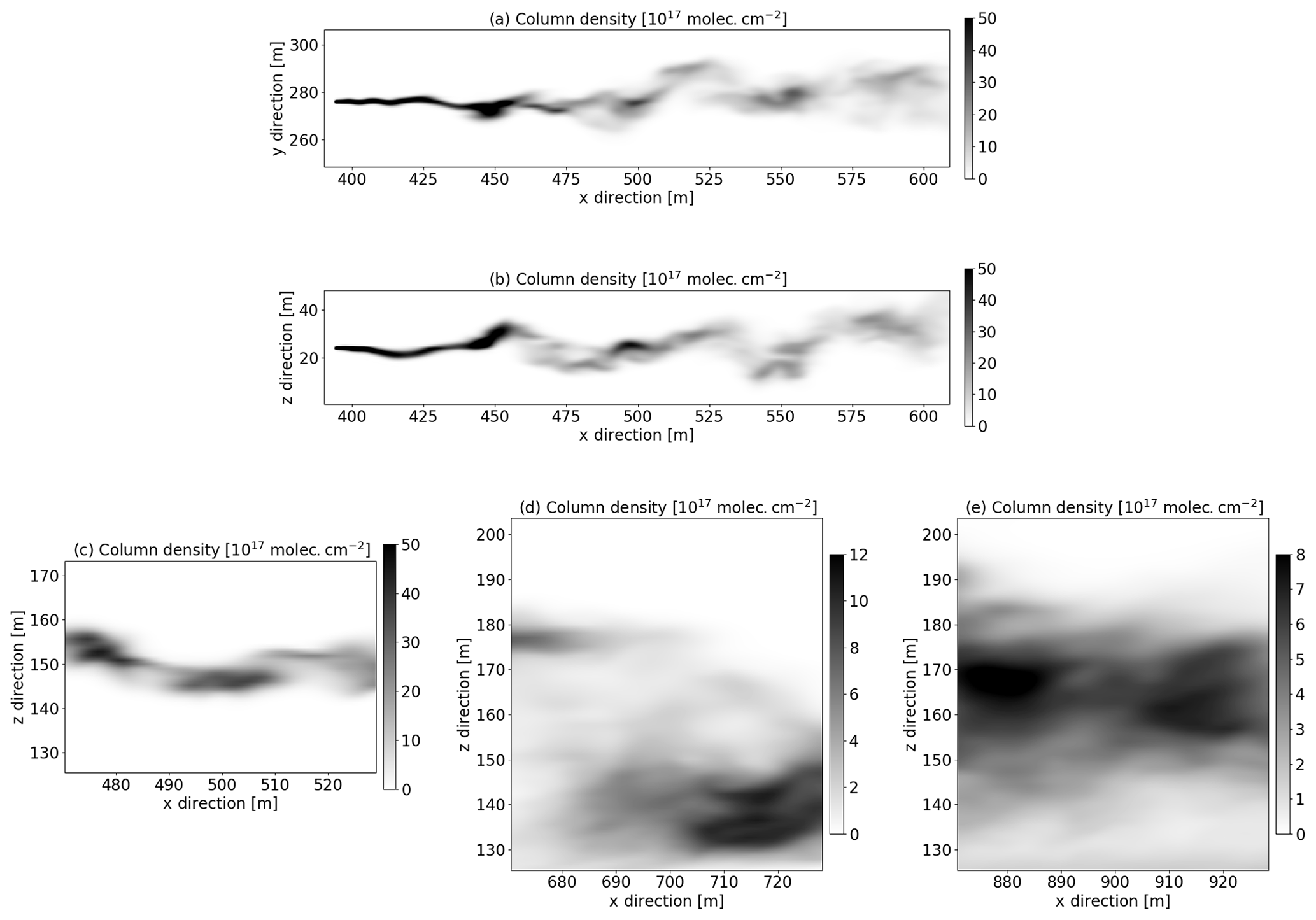
Figure 1 (a) SO₂ column densities from the LES (time frame no. 2) integrated along the vertical z direction. This corresponds to the part of the plume viewed by camera A. (b) Corresponding SO₂ column densities integrated along the crosswind y direction. (c–e) LES SO₂ column densities (time frame nos. 61, 10, and 91) integrated along the crosswind y direction, corresponding to the part of the plume viewed by cameras B, C, and D, respectively. Note the different scales of the greyscale bars.

2.2 Radiative transfer simulations

The UV camera images were simulated with the 3D MYSTIC Monte Carlo radiative transfer model which was run within the libRadtran framework (Mayer et al., 2010; Emde et al., 2010, 2016; Buras and Mayer, 2011; Mayer and Kylling, 2005). MYSTIC includes an option to calculate the radiation impinging on a camera with a prescribed number of pixels in a plane defined by the location of the camera within a 3D domain and the camera viewing direction. For this option, the MYSTIC Monte Carlo model is run in backward mode. The MYSTIC camera simulation capabilities have earlier been used by, for example, Kylling et al. (2013) to simulate infrared satellite images. Here it is used to simulate radiative transfer to a UV camera at wavelengths suitable for the detection of SO₂. Thus, for each camera pixel, spectra were calculated for wavelengths ranging between 300 and 350.5 nm. The spectral resolution was 0.1 nm in order to capture the fine structure of the SO₂ cross section. The spectra were weighted with spectral response functions (about 10 nm width) representing cameras with mounted on-band (sensitive to SO₂ absorption, centred at 310 nm) and off-band (barely sensitive to SO₂ absorption, centred at about 330 nm) filters similar to those described by Gliß et al. (2018). Quantum efficiency of the detector and geometrical effects related to lens/camera optics were not included in the camera simulations. SO₂ plume concentrations were adopted from the LES simulations described in Sect. 2.1, and the spectrally dependent SO₂ absorption cross section was taken from Hermans et al. (2009).

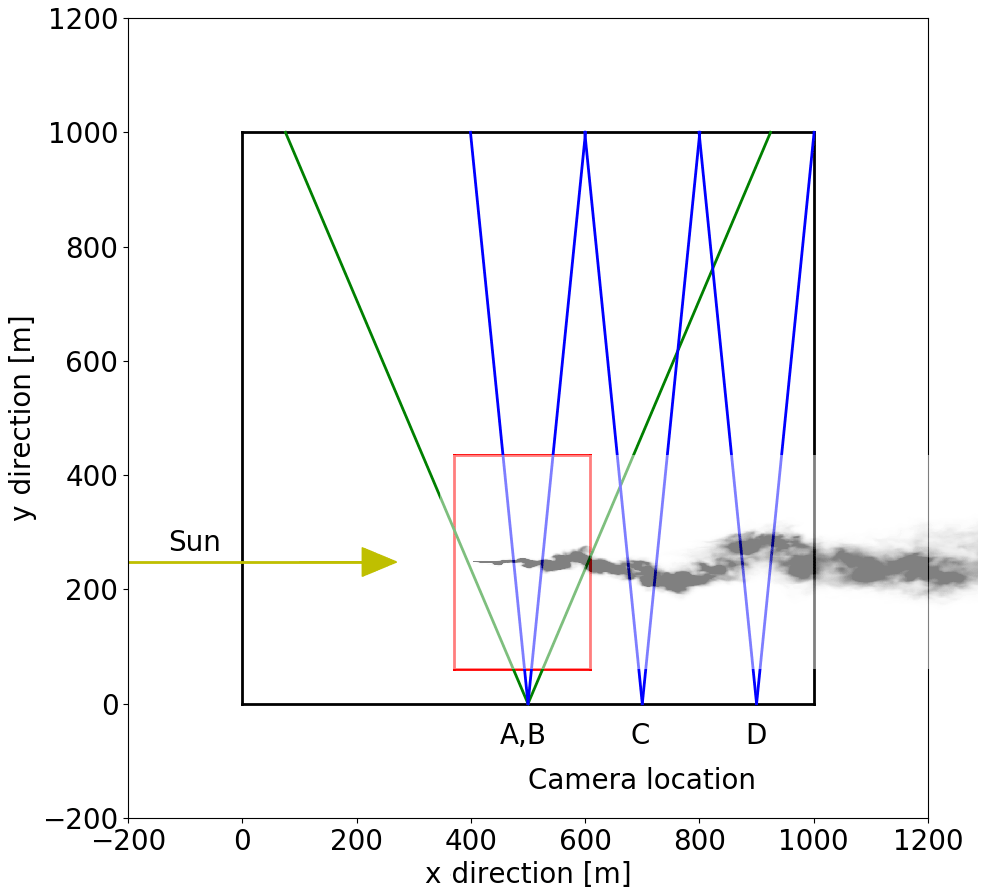
Figure 2 Bird's eye view of the 3D domain (black square) and the SO₂ plume location within the domain (red square for camera A simulation, shifted along x axis for the other cameras). The UV cameras are located where the two green or blue lines intersect. The lines indicate the horizontal field of view of the cameras, and their locations are given in Table 1. The column density (similar to Fig. 1a) of the plume is included for illustrative purposes. The direction of the incoming sunray is shown by the yellow line.

A finite 3D domain (bird's eye view provided in Fig. 2) is defined for the radiative transfer simulations. The SO₂ plume is embedded in this domain and is viewed from the side at a distance of about 250 m by the UV camera, which is placed 1 m above the surface. This camera–plume distance is comparable to that used during part of the first COMTESSA field campaign described by Dinger et al. (2018).

Four different cameras at different locations and viewing geometries were simulated. These are summarized in Table 1.

Table 1 Location and geometric specification of the four simulated cameras. All cameras were placed 1 m above the surface.

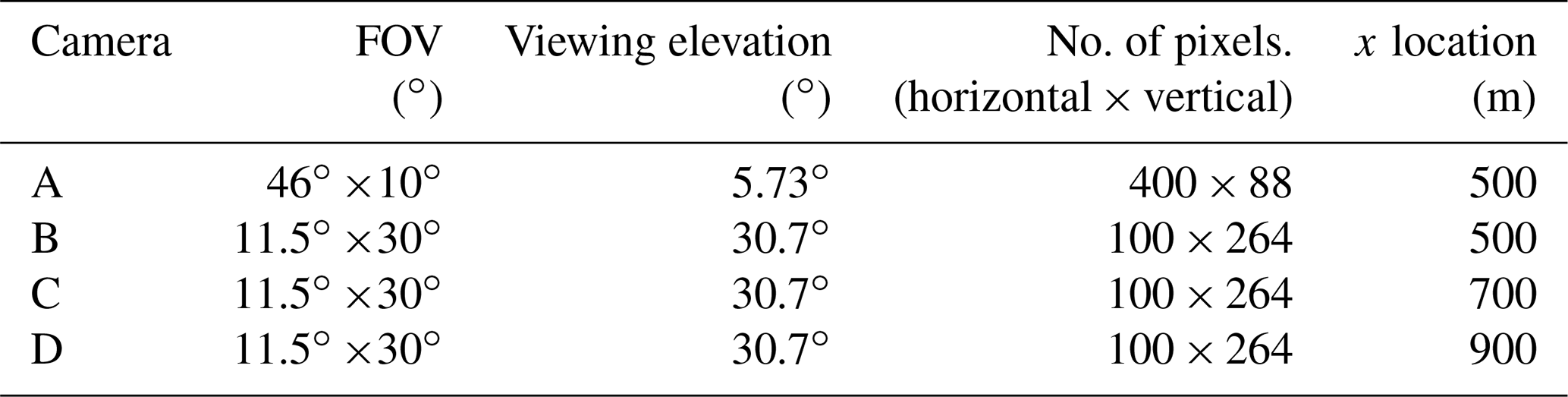
Camera A captures the plume from its release point and about 200 m downwind. It sees the plume released at an altitude of 25 m and thus has a low-angle viewing elevation; see Table 1. Cameras B, C, and D resemble a different experimental situation with the plume release altitude of 150 m. These cameras thus have a larger viewing elevation. Camera B is placed at the same x-direction location as camera A but has a smaller horizontal field of view (FOV) to focus on the more mature parts of the plume. Cameras C and D are placed further downwind and view the plume about 300 and 500 m downwind from the release point, respectively.

The LES voxel resolution is about 1 m³, which at a distance of 250 m corresponds to 0.004 rad=0.23^∘. To ensure sufficient spatial sampling, the camera resolution was specified to be about half the LES voxel resolution. To be able to see the plume at the various camera positions the camera FOV was varied and the number of pixels adopted to give a camera resolution of about 0.5 m at the plume. It is noted that the UV cameras used by Dinger et al. (2018) had 1392×1040 pixels. The reason and justification for using fewer pixels in the simulated camera are twofold: (1) with the simulated camera it is possible to zoom onto the plume as one always knows where the plume is. In an experimental setting, the plume usually covers only part of the FOV to allow for changes in wind direction and, thus, changes in plume position. (2) The computer time and memory requirements increase as the number of pixels increases. It is thus advantageous to use as few pixels as needed to cover the plume.

As the COMTESSA field campaigns are being carried out primarily in central Norway during the summer time, solar zenith angles of 40^∘ and 60^∘ were considered. When not otherwise noted (see Sect. 3.2), the sun was assumed to be perpendicular to the camera viewing direction; see Fig. 2.

To further save computer memory and time, a full 3D description of the plume is given only in the part of the domain containing the plume seen by the camera (red square in Fig. 2). Outside the red square, the plume is not included. Energy conservation is ensured by using periodic boundary conditions; that is, photons leaving the domain on one side enter the domain again on the opposite side. Not having periodic boundary conditions would let the photons leave the domain and thus not be accounted for. Periodic boundary conditions imply that effectively the plume within the domain keeps on repeating itself in the horizontal. Thus the plume may be seen by the camera several times if care is not taken when setting up the geometry of the computational domain, the location of the plume within the domain, and the camera. However, sometimes these “ghost” plumes are unavoidable due to the geometry and computational resources. It is noted that the “ghost” plumes get smaller and smaller in the camera view the further away they are from the domain with the camera. For camera A “ghost” plumes pose a challenge due to the low-altitude plume and camera viewing angles close to the horizon. Great care was thus taken when setting the domain size and the camera A field of view to avoid “ghost” plumes in the simulated images. Still, part of a secondary “ghost” plume is present in some of the images. These “ghost” plumes have been removed from the analysis presented below for camera A.

For representing the ambient atmosphere, the mid-latitude summer atmosphere of Anderson et al. (1986) was used. The surface albedo is small in the UV for non-snow-covered surfaces and was thus set to zero when not otherwise noted (see Sect. 3.4). Aerosols were included for specific sensitivity tests that are described in Sect. 3.3.

The radiative transfer simulations were run on a Linux cluster utilizing 10 processors in parallel, with each process needing about 10–15 GB of memory depending on whether aerosols in the plume were included or not. The MYSTIC Monte Carlo radiative transfer simulation is statistical in nature, and the simulated images thus contain statistical noise. To achieve a noise level of about the same order of magnitude as the measurements (≈1 %), a sufficient number of photons needs to be traced. For each pixel and wavelength 2000 photons were traced. This gave simulation times for one on- and one off-band image of about 120–140 h and ensured that, for the simulations without aerosol and zero surface albedo, at least 93.0 % of the pixels had radiances with a relative standard deviation <1.0 %. For simulations with background aerosols, the corresponding number is 83 %.

2.3 Analysis methodology

The apparent absorbance for the on-band camera is given by Mori and Burton (2006) and Lübcke et al. (2013) as follows:

$$\begin{array}{}\text{(1)}& {\mathit{\tau }}_{\mathrm{on}}=-\ln {\displaystyle \frac{I_{\mathrm{on},M}}{I_{\mathrm{on},\mathrm{0}}}}.\end{array}$$

Here, I_on,M is the on-band radiance and I_on,0 the background radiance without the SO₂ plume. In addition to absorption by SO₂, τ_on may include absorption due to aerosol and plume condensation. Assuming that the absorption by these other constituents varies little with wavelength between the on- and off-band cameras, the extra absorption may be removed by subtracting the off-band absorption as follows:

$$\begin{array}{}\text{(2)}& \begin{array}{rl}\mathit{\tau }& ={\mathit{\tau }}_{\mathrm{on}}-{\mathit{\tau }}_{\mathrm{off}}=-\ln {\displaystyle \frac{I_{\mathrm{on},M}}{I_{\mathrm{on},\mathrm{0}}}}+\ln {\displaystyle \frac{I_{\mathrm{off},M}}{I_{\mathrm{off},\mathrm{0}}}}\\ & =\ln \left({\displaystyle \frac{I_{\mathrm{off},M}}{I_{\mathrm{on},M}}}{\displaystyle \frac{I_{\mathrm{on},\mathrm{0}}}{I_{\mathrm{off},\mathrm{0}}}}\right),\end{array}\end{array}$$

where I_off,M and I_off,0 are the off-band radiance and the off-band background radiance, respectively. The background images were calculated similar to the plume images but with the SO₂ concentration set to zero. Below, plume statistics are presented for both τ_on and τ.

Ideally, plume statistics from the LES SO₂ concentrations and image-derived SO₂ concentrations should be compared. However, for the images this would require simulating the geometry suitable for tomography and tomographic reconstruction of the plume. The slant column density (SCD) is the concentration of a gas along the light path (typically in units of m⁻²). It is calculated from the LES SO₂ concentrations by tracing individual rays corresponding to individual camera pixels. From apparent absorbances, the SCD may be retrieved. For SO₂ camera measurement this is done by calibrating the camera with SO₂ cells and/or concurrent differential optical absorption spectroscopy (DOAS) measurements. The calibration gives a linear relationship between the apparent absorbance and the SCD (see, for example, Lübcke et al., 2013). Such calibration procedures could be simulated and used to calibrate the simulated images. However, higher-order moments (first-order moment and upwards) would be the same for the SCD and the apparent absorbance due to the linear relationship between the two. Thus, below we will compare SO₂ SCD from the LES with apparent absorbance from the images. We note that this comparison will not include the zeroth moment (total mass) and that systematic biases may go undetected. While a comparison of the total mass certainly is of interest, this would require a systematic investigation of SO₂ calibration using simulated images, which is beyond the scope of this work.

2.3.1 Plume statistics

For projected LES simulations and the simulated images, the vertical (in the images) plume centre-line position, meandering, absolute and relative dispersions, and the skewness were calculated (see e.g. Dosio and de Arellano, 2006). However, the absolute dispersion can only be properly defined using an ensemble or time average. As this is not possible here due to the above-mentioned computing limitations, we use the centre of the source ($\stackrel{\mathrm{‾}}{z}=z_{\mathrm{0}}$) as the reference vertical position.

Each pixel in the camera images and each projection from the LES simulations describe the integrated column amount (ρ_L) of the trace gas along the line of sight (dL) as follows:

$$\begin{array}{}\text{(3)}& {\mathit{\rho }}_L=\int \mathit{\rho }\mathrm{d}L,\end{array}$$

where ρ is the density of the trace gas. The instantaneous vertical plume centre-line position z_m is given by the following:

$$\begin{array}{}\text{(4)}& z_{\mathrm{m}}\left(x\right)={\displaystyle \frac{\int z{\mathit{\rho }}_L\mathrm{d}z}{\int {\mathit{\rho }}_L\mathrm{d}z}},\end{array}$$

where x and z are the horizontal and vertical positions of the pixel, respectively.

The fluctuations of the absolute, relative, and centre-line positions are defined as follows:

$$\begin{array}{}\text{(5)}& {\displaystyle }{z}^{\prime }=z-z_{\mathrm{0}}\text{(6)}& {\displaystyle }{z}_{\mathrm{r}}=z-z_{\mathrm{m}}\text{(7)}& {\displaystyle }{z}_{\mathrm{m}}^{\prime }=z_{\mathrm{m}}-z_{\mathrm{0}}.\end{array}$$

It is noted that with this definition of the absolute position, relative and absolute dispersion are the same at the source location, since meandering here is zero. Also, since we set $\stackrel{\mathrm{‾}}{z}=z_{\mathrm{0}}$, there will be correlations between $z_{\mathrm{m}}^{\prime }$ at different x, which also implies that $\stackrel{\mathrm{‾}}{\left(z_{\mathrm{m}}^{\prime }\right)}$ is strictly speaking not a robust reference for defining meandering of the plume. However, the purpose of this study is to investigate the sensitivity of the statistical properties to changes in various atmospheric parameters and this limitation should have minimal impact on the results.

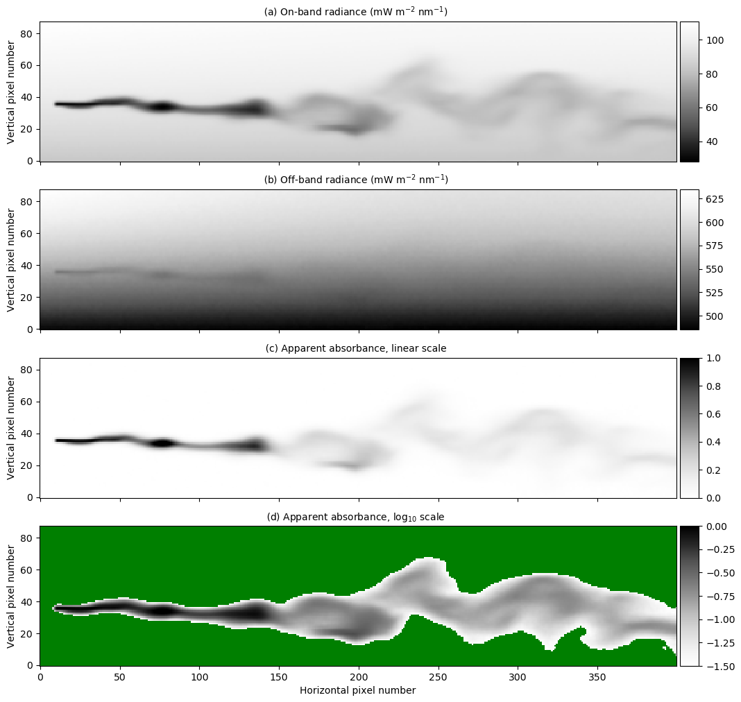
Figure 3 Radiances and apparent absorbance for camera A, with the same time frame as in Fig. 1. (a) The on-band radiance. (b) The off-band radiance. (c) The apparent absorbance calculated using Eq. (2). (d) Same as (c) but with logarithmic greyscale. The green colouring represents pixels for which the apparent absorbance τ<0.03.

The absolute (σ_z), relative (σ_zr), and meandering (σ_zm) dispersions are defined as follows:

$$\begin{array}{}\text{(8)}& {\displaystyle }{\mathit{\sigma }}_z^{\mathrm{2}}\left(x\right)={\displaystyle \frac{\int {\mathit{\rho }}_L{z}^{\prime \mathrm{2}}\mathrm{d}z}{\int {\mathit{\rho }}_L\mathrm{d}z}}\text{(9)}& {\displaystyle }{\mathit{\sigma }}_{z\mathrm{r}}^{\mathrm{2}}\left(x\right)={\displaystyle \frac{\int {\mathit{\rho }}_L{z}_{\mathrm{r}}^{\mathrm{2}}\mathrm{d}z}{\int {\mathit{\rho }}_L\mathrm{d}z}}\text{(10)}& {\displaystyle }{\mathit{\sigma }}_{z\mathrm{m}}^{\mathrm{2}}={\displaystyle \frac{\int {\mathit{\rho }}_L{z}_{\mathrm{m}}^{\prime \mathrm{2}}\mathrm{d}x}{\int {\mathit{\rho }}_L\mathrm{d}x}}\end{array}$$

and similarly for the skewnesses, as follows:

$$\begin{array}{}\text{(11)}& {\displaystyle }\stackrel{\mathrm{‾}}{z^{\prime \mathrm{3}}}={\displaystyle \frac{\mathrm{1}}{{\mathit{\sigma }}_z^{\mathrm{3}}\left(x\right)}}{\displaystyle \frac{\int {\mathit{\rho }}_L{z}^{\prime \mathrm{3}}\mathrm{d}z}{\int {\mathit{\rho }}_L\mathrm{d}z}}\text{(12)}& {\displaystyle }\stackrel{\mathrm{‾}}{z_{z\mathrm{r}}^{\prime \mathrm{3}}}={\displaystyle \frac{\mathrm{1}}{{\mathit{\sigma }}_{z\mathrm{r}}^{\mathrm{3}}\left(x\right)}}{\displaystyle \frac{\int {\mathit{\rho }}_L{z}_{\mathrm{r}}^{\mathrm{3}}\mathrm{d}z}{\int {\mathit{\rho }}_L\mathrm{d}z}}\text{(13)}& {\displaystyle }\stackrel{\mathrm{‾}}{z_{z\mathrm{m}}^{\prime \mathrm{3}}}={\displaystyle \frac{\mathrm{1}}{{\mathit{\sigma }}_{z\mathrm{r}}^{\mathrm{3}}\left(x\right)}}{\displaystyle \frac{\int {\mathit{\rho }}_L{z}_{\mathrm{m}}^{\prime \mathrm{3}}\mathrm{d}x}{\int {\mathit{\rho }}_L\mathrm{d}x}}.\end{array}$$

These various quantities were calculated both directly from the projected LES simulations and also from the camera images. The former served as a reference (“ground truth”) against which the quantities derived from the camera images were compared.

Figure 4 (a) The plume apparent absorbance for camera A from Fig. 3c. (b) The LES column density integrated along the line of sight. Colour scales in (a) and (b) are relative and thus no colour bars are provided. (c) The centre line, absolute, and relative dispersions. (d) The skewness.

3 Results

We first compare statistical results from the LES and simulated images reference atmospheric conditions. This comparison is made for multiple time frames and is done in order to estimate how well the camera-derived statistics may reproduce the LES statistics. Next the impact of solar angles, aerosol load, and surface albedo on plume statistics is investigated for a single time frame.

3.1 Reference cases

Figure 3a and b show simulated on- and off-band radiances, respectively, for camera A and the reference case (no aerosol, zero surface albedo, and a solar zenith angle of 40^∘).

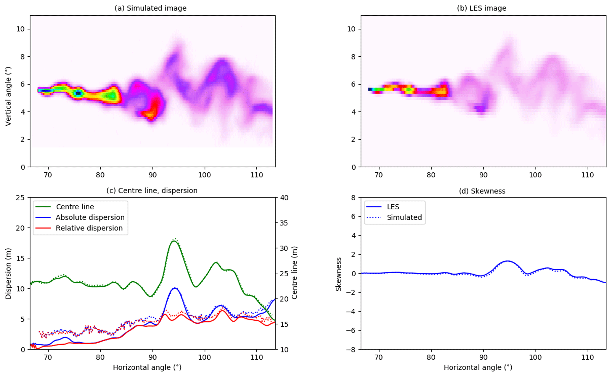
The strong absorption of SO₂ in the on-band image is clearly visible in Fig. 3a. There is also a weak SO₂ signal in the off-band image (Fig. 3b). From the on- and off-band images and corresponding background images not including the SO₂ plume, the apparent absorbance was calculated using Eq. (2). The resulting apparent absorbance is shown in Fig. 3c on a linear scale and in Fig. 3d on a logarithmic scale. The apparent absorbance is reproduced in Fig. 4a, while Fig. 4b shows the SCD calculated along the line of sight using the LES concentrations. The plume centre line, absolute and relative dispersions, and skewness, as defined in Eqs. (4), (8), and (11), were calculated from the simulated images and the LES images. These are shown as solid lines (LES) and dotted lines (camera simulation) in Fig. 4c and d. Similar plots for cameras B, C, and D are presented in Figs. 5–7. Note that the simulated and LES images in Figs. 4–7 differ from those in Fig. 1 due to different viewing directions. In the latter the plumes are viewed at a viewing angle of 0^∘ while for cameras A, B, C, and D the viewing angle differs from the horizontal; see Table 1.

Figure 5 Similar to Fig. 4 but for camera B and time step 61.

Figure 6 Similar to Fig. 4 but for camera C and time step 10.

Figure 7 Similar to Fig. 4 but for camera D and time step 91.

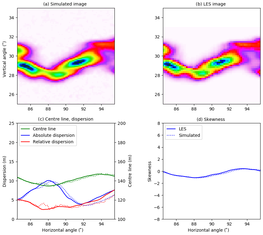
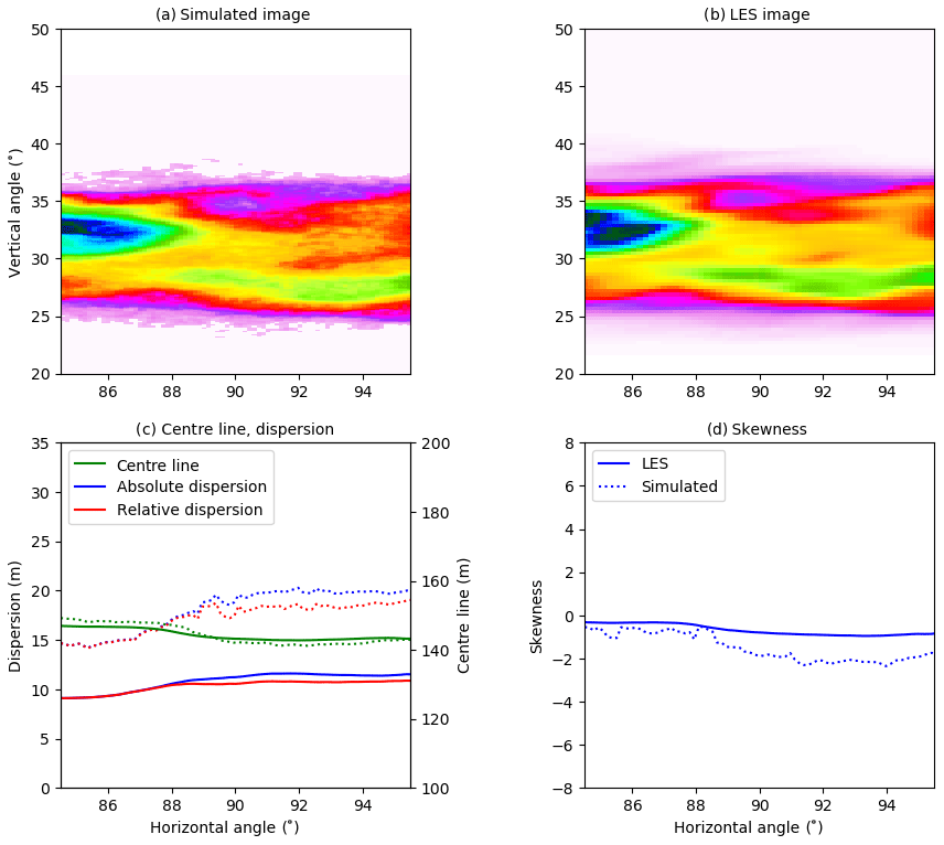
Overall the behaviour of the centre line, absolute and relative dispersions, and skewness calculated from the simulated images is similar to those from the LES densities for all cameras. The centre line agrees well for all four cameras. For camera A, Fig. 4, the absolute and relative dispersions from the camera are larger than those from the LES for the plume downwind to about 100 m (corresponding to ≈90^∘ horizontal viewing angle) from the release point. For camera B, Fig. 5, all quantities agree well, while for cameras C (Fig. 6) and D (Fig. 7), the camera dispersions are larger than the LES dispersions by about 50 %–60 %, and the magnitude of the skewness from the camera is also larger.

To shed further light on the differences between the images from the radiative transfer simulation and the LES, we show the probability density function (pdf) of the column densities from the LES and simulated images in Fig. 8. These pdf's represent area sample pdf's and cover the full images.

Figure 8 The probability density function (pdf) of the column densities from the LES and simulated images in Figs. 4–7.

For camera A the pdf's differ for intermediate values, where an artificial secondary peak is created in the pdf for the simulated image. This is most likely due to the diffusive nature of the radiative transfer in the young part of the plume (horizontal angle smaller than about 85^∘) where the LES plume is of the size a few voxels. However, the SO₂ absorption signal is strong, and thus the centre line, dispersions, and skewness agree well for the dispersed part of the plume. For camera B the pdf's are similar, and this is reflected in the good agreement between the statistical quantities presented in Fig. 5. This indicates that when the plume is large enough compared to the pixel resolution the camera can capture the plume well. The pdf's for camera C exhibit much the same behaviour. However, at this further downwind location, the plume is more dispersed, and the SO₂ absorption signal is weaker and sometimes beyond detection (thus the lower cut-off in the pdf of the simulated image). The weaker absorption signal implies that the statistical noise from the Monte Carlo-based radiative transfer simulation becomes discernible and increases the dispersions compared to the LES (Fig. 6). A similar situation is evident for camera D; see pdf's in Fig. 8 and statistical quantities in Fig. 7.

As noted above, a large number of images such as in Fig. 3 is required to estimate the parameters of interest for the description of turbulence. This is not computationally feasible with the available resources. However, it is noted that if the instantaneous statistics are correct, the ensemble statistics will also be correct. This is not necessarily true the other way around. To provide an estimate of the difference between the statistical quantities from the simulated images and the LES densities, the differences between the centre line, the absolute and relative dispersions, and the skewness were calculated for seven (camera A) and nine (cameras B, C, and D) random time steps. The mean differences and the standard deviations are summarized in Table 2.

Table 2 The mean ± the standard deviation for the difference between the simulated images and the LES densities for seven (camera A) and nine (cameras B, C, and D) randomly chosen time steps.

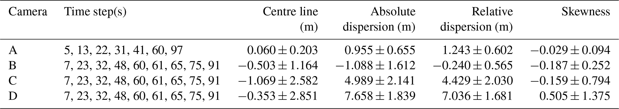
The mean differences between the quantities from the simulated images and the LES densities are small for cameras A and B. For the centre line and the dispersions the differences are about or smaller than the voxel resolution of the LES simulations. For camera C the centre-line differences are about the LES voxel resolution, whereas the dispersion differences increase. Camera D differences show similar behaviour but with even larger differences for the dispersions. As already mentioned above, the main source for the differences is the Monte Carlo noise in the radiative transfer simulation when the SO₂ signal becomes weak. This alters the dispersions, Figs. 4–7, and pdf's, Fig. 8. This is evident in the simulated images dispersions, which are not as smooth as those from the LES (Figs. 5–7). It must also be emphasized that the densities simulated by the LES and the apparent absorbance are not the same physical quantities but are non-linearly connected through the radiative transfer equation.

3.2 Solar azimuth and zenith angle effects

In Figs. 3 and 4 results were shown for solar azimuth and zenith angles of ϕ₀=90^∘ and θ₀=40^∘, respectively. The simulations were repeated for a solar zenith angle of θ₀=60^∘ to see if this would change the plume statistics. The difference in apparent absorbance, $\mathit{\delta }\mathit{\tau }=\mathit{\tau }({\mathit{\theta }}_{\mathrm{0}}=\mathrm{60})-\mathit{\tau }({\mathit{\theta }}_{\mathrm{0}}=\mathrm{40})$, is shown in Fig. 9.

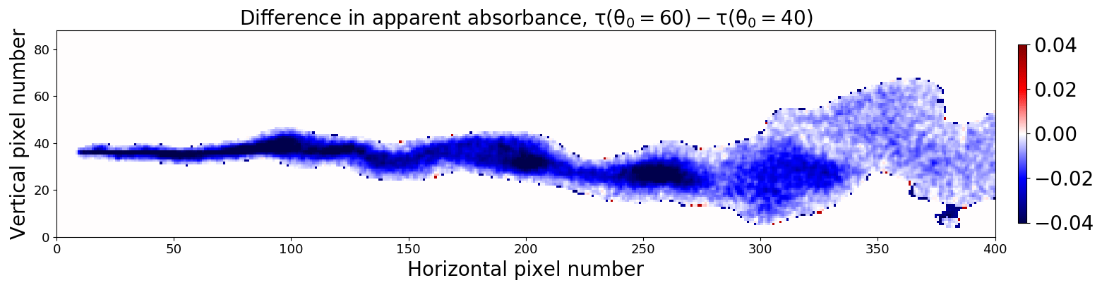
Figure 9 The difference in apparent absorbance from images recorded at two different solar zenith angles, namely θ₀=60^∘ and θ₀=40^∘.

The apparent absorbance is generally slightly smaller (on average about 6 %) for θ₀=60^∘ than for θ₀=40^∘. Ideally the apparent absorbance is due to photons travelling along straight lines passing through the plume and into the camera. However, photons taking other paths may also contribute to the signal. Direct solar radiation photons contribute in the following three ways to the camera signal through: (1) direct photons scattered behind the plume in the direction of the camera; (2) direct photons scattered in the plume towards the camera; and (3) direct photons scattered between the plume and the camera in the direction of the camera. The first part is included in the apparent absorbance and does not depend on solar zenith angle due to the background correction. The third part is called light dilution and does not depend on the amount of SO₂ in the plume. The second part depends on the amount of SO₂ in the plume and the solar zenith angle. The latter is because there is relatively more direct radiation at θ₀=40^∘ than at θ₀=60^∘. Hence, more direct radiation is likely to enter the plume for θ₀=40^∘ and be scattered into the camera from inside the SO₂ plume. This explains the negative difference in the apparent absorbance between θ₀=60^∘ and θ₀=40^∘. It is noted that in an experimental setting, where calibrations are carried out throughout the day, solar zenith angle variations will not necessarily give a change in SO₂.

Statistics were calculated as for the θ₀=40^∘ case and differences to this case are summarized in Table 3, with rows labelled “θ₀=60^∘”. In the table, differences are reported as the maximum difference in units of metres. Differences are reported both without and with the off-band correction (Eqs. 1 and 2, respectively) to quantify the impact of the correction. Overall, the statistics for the θ₀=60^∘ results deviate little from the θ₀=40^∘ case. The difference in meandering, not shown in Table 3, is negligible for this and all sensitivity cases below and is not further discussed.

Table 3 Summary of differences in statistics between the baseline case shown in Fig. 4 and the sensitivity tests (first column). The second column reports the mean and standard deviation (SD) of the difference in absorbance (δτ). For the centre line, absolute dispersion, and relative dispersion, the mean and standard deviation (SD) are given in units of metres. For the azimuth dependence sensitivity, tests were made for a range of angles; the numbers in the table are the extreme values for all these tests.

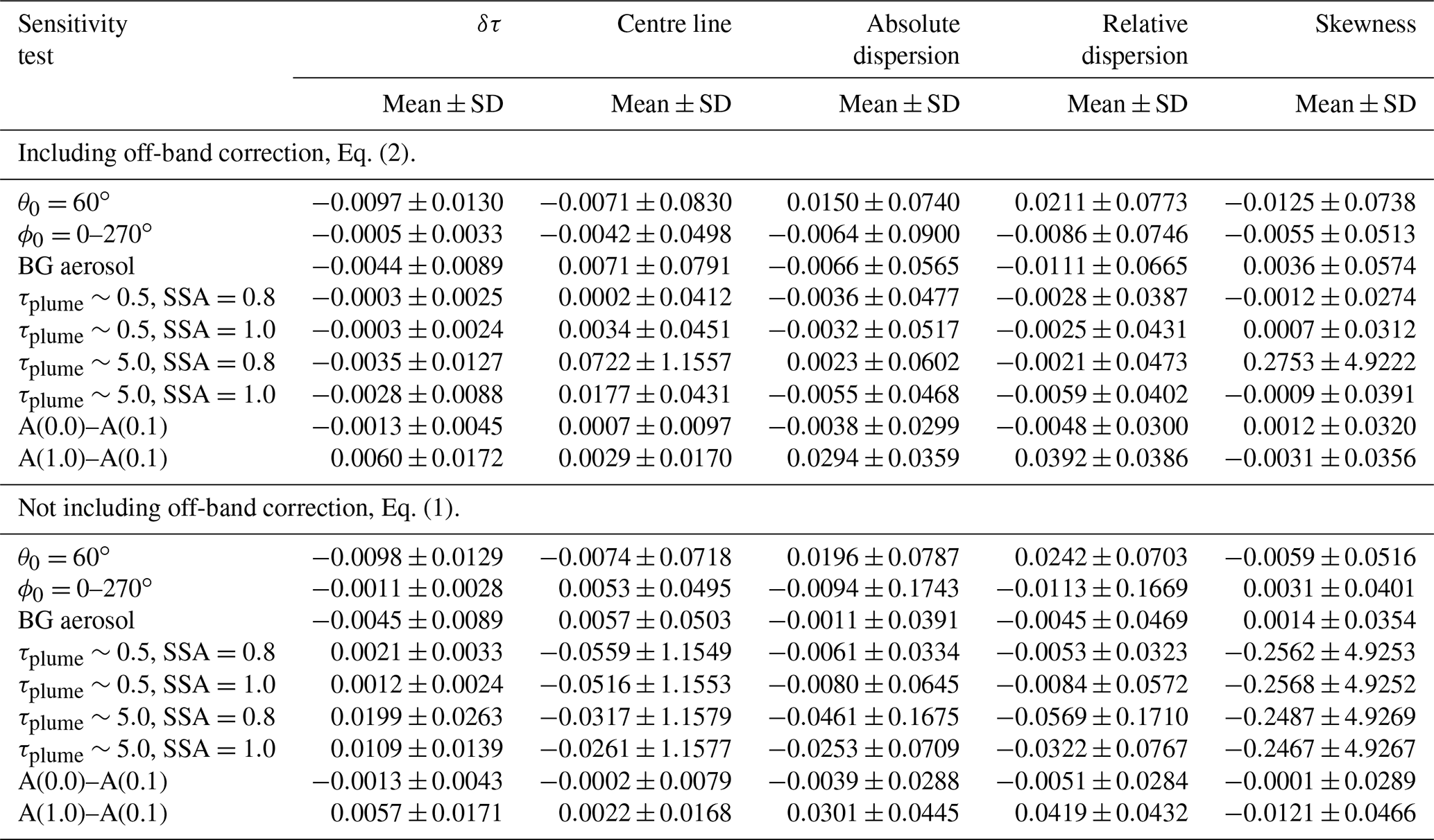
The sensitivity to the solar azimuth angle was investigated by setting the solar azimuth angle to ϕ₀=0, 45, 135, 180, and 270^∘, while keeping the solar zenith angle at θ₀=40^∘. The difference in absorbance is less than 0.05 % on average. The impact on the centre line, absolute and relative dispersions, and skewness is negligible; see rows labelled “ϕ₀=0–270^∘” in Table 3. From the results no preferable solar azimuth camera viewing direction geometry may be identified. However, note that the azimuth angle of the background image needs to be the same as for the image with SO₂. It is noted that including aerosols has negligible effect on the solar azimuth angle sensitivity; see Sect. 3.3.

3.3 Aerosol effects

No aerosols were included in the simulations above. Background aerosols may be present in both the plume and in the surrounding atmosphere. Furthermore, aerosol may be present in the plume due to formation of sulfate aerosol from SO₂. Both cases are investigated below.

First, background aerosol with an optical depth t_BG(310)=0.5 and a single scattering albedo (SSA) of about 0.95 at 310 nm were included in simulations for θ₀=40^∘ (the aerosol_default option of uvspec was used; see Emde et al., 2016). The difference between the simulation including background aerosol and the aerosol-free simulation is shown in Fig. 10a.

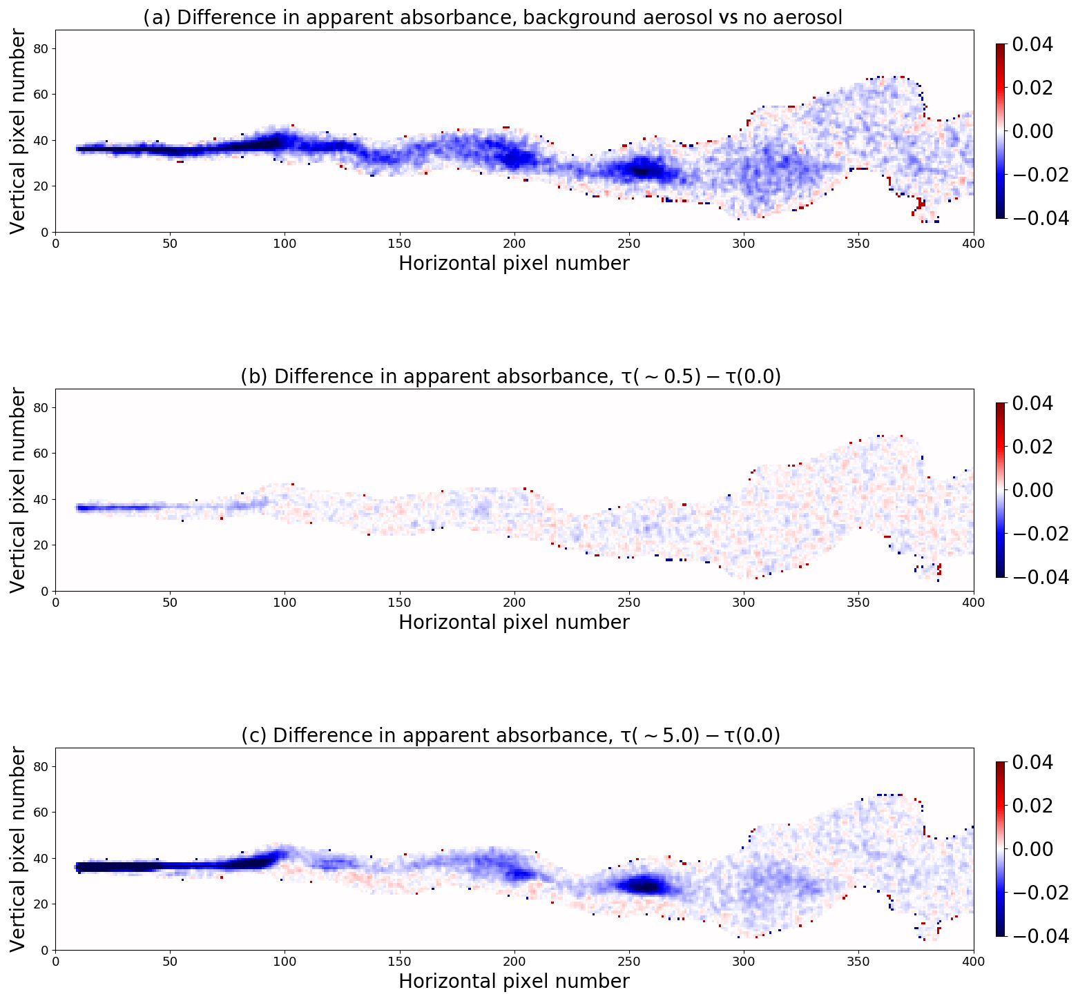
Figure 10 The difference in apparent absorbance from images recorded (a) with and without background aerosols in the atmosphere and (b–c) with and without aerosol in the plume. (b) τ_plume∼0.5 and (c) τ_plume∼5.0.

Including background aerosol generally gives a slightly lower apparent absorbance, which is on average about 2.5 % whether the off-band correction is excluded or included (Eqs. 1 and 2, respectively). The decrease is due to multiple scattering by the aerosol and hence less direct radiation (Kern et al., 2010a). The background aerosol had negligible effects on plume statistics (Table 3, rows labelled “BG aerosol”).

Simulations were also made with aerosol in the plume only; that is, various amounts of aerosol were added to the voxels containing SO₂. This is relevant for non-pure SO₂ plumes where aerosols are co-emitted, such as from power plants, or where secondary sulfate aerosols may form in the SO₂ plume. The impact of both highly absorbing (SSA=0.8) and purely scattering aerosol (SSA=1.0) was investigated. Kern et al. (2013) concluded that if a plume contains an absorbing aerosol component the retrieved SO₂ columns may be underestimated. Here we estimate the effect of aerosols in the plume on the higher-order statistics of the plume. Figure 10b and c show the difference in apparent absorbance between simulations with and without absorbing aerosol in the plume for a relatively large aerosol optical depth of about 0.5 (Fig. 10b) and an unrealistic extreme case with aerosol optical depth of about 5.0 at 310 nm (Fig. 10c). Results for non-absorbing aerosol are similar (not shown).

For the more realistic value, τ_plume∼0.5, Fig. 10b, there is little impact on the apparent absorbance. For (non-)absorbing aerosol with SSA=0.8 (SSA=1.0), the decrease is less than 0.2 % (0.16 %) on average with off-band correction, and the increase is less than 1.1 % (0.63 %) on average without off-band correction. For (unrealistically) large amounts of (non-)absorbing aerosol in the plume, τ_plume∼5.0, the apparent absorbance decreases by less than 2 % (1.5 %) on average if off-band correction is included; see Eq. (2). Without off-band correction, Eq. (1), the apparent absorbance increases by 9.5 % (5.43 %) on average. For all cases the off-band correction reduces the influence of aerosol, as intended. For both aerosol in plume cases and whether the off-band correction was included or not, the plume statistics were affected to a negligible extent, as reported in rows labelled “τ_plume” in Table 3. However, the standard deviation of the skewness increases largely when aerosol influence is not corrected for or if the plume is thick and absorbing.

The sensitivity of the solar azimuth angle when including aerosols was investigated by performing additional simulations for ϕ₀=45 and 180^∘ for the aerosol in the plume and background aerosol cases with τ_plume∼0.5. The solar azimuth angle sensitivity for these cases were of the same magnitude as for the aerosol-free simulations and thus of negligible impact.

3.4 Surface albedo

All simulations above were made with a surface albedo A=0.0 to avoid coupling between the various processes that affect the camera images. For the wavelengths considered here the albedo for snow-free surfaces is generally small (A<0.1; see for example Wendisch et al., 2004). To test the sensitivity to snow-free surface albedo, simulations were made for surface albedos of A=0.05 and A=0.1. In addition, a simulation was made with A=1.0 to estimate the effect of fresh snow which has an albedo close to one at UV wavelengths (Wiscombe and Warren, 1980). The background images were calculated for each individual case. The apparent absorbance difference for the A(0.0)–A(0.1) and A(1.0)–A(0.1) cases is shown in Fig. 11.

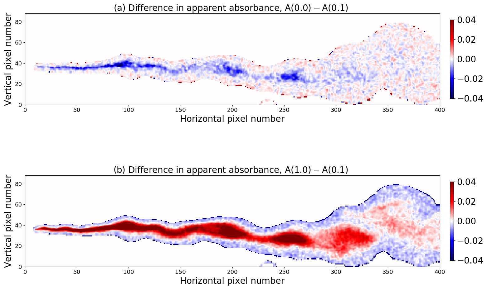
Figure 11 The difference in apparent absorbance from images recorded with a surface albedo of (a) A(0.0) and A(0.1) and (b) A(1.0) and A(0.1).

The overall results are summarized in Table 3. Decreasing the albedo from 0.1 to 0.0 gives an overall reduction in the apparent absorbance (mostly blue colours in Fig. 11a). Compared to the A=0.1 case, the A=0.05 case, not shown, is about a factor of 2 smaller in magnitude for the mean apparent absorbance. Increasing the albedo from 0.1 to 1.0 gives an increase in the apparent absorbance (mostly red colours in Fig. 11b). As mentioned above, Sect. 3.2, the apparent absorbance is due to photons travelling along straight lines passing through the plume and into the camera. However, photons scattered between the plume and the camera, and multiple scattered photons within the plume, termed the light dilution and multiple scattering effect, respectively, may distort the apparent absorbance (Kern et al., 2012). An additional distortion, not discussed by Kern et al. (2012), is due to the surface albedo which gives additional photon paths that may contribute to the camera signal. Some photons may scatter off the surface into the plume and in the direction of the camera. This will give increased (decreased) apparent absorbance with increasing (decreasing) albedo for relatively large SO₂ concentrations; see red (blue) signal in Fig. 11b (a). For small SO₂ concentrations, the light dilution effect prevails, giving a reduction (increase) in the apparent absorbance for increasing (decreasing) albedo; see blue (red) signal in Fig. 11b (a). While albedo changes may both increase and decrease the apparent absorbance, the impact on plume statistics is minor. Thus, overall, the surface albedo has negligible effect on the plume statistics (Table 3).

4 Conclusions

One novel method to measure atmospheric turbulent tracer dispersion is to use UV cameras sensitive to absorption of sunlight by SO₂. In this paper we have presented a method to simulate such UV camera measurement with a 3D Monte Carlo radiative transfer model. Input to the radiative transfer simulations are large eddy simulations (LES) of a SO₂ plume. From the simulated images, various plume density statistics (centre-line position, meandering, absolute and relative dispersions, and skewness) were calculated and compared with similar quantities directly from the LES. Mean differences between the simulated images and the LES were generally found to be smaller or about the size of the voxel resolution of the LES for the centre line. For the higher-order statistics, the differences increase as the SO₂ absorption gets weaker for a more and more dispersed plume.

Furthermore, sensitivity studies were made to quantify how changes in solar azimuth and zenith angles, aerosol (background and in plume), and surface albedo impact the UV camera image plume statistics. It was found that changing the parameters describing these effects within realistic limits had negligible effects on the centre-line position, meandering, absolute and relative dispersions, and skewness of the SO₂ plume.

Based on the simulated UV camera images and the comparison with the LES, it can be concluded that UV camera images of SO₂ plumes may be used to derive plume statistics of relevance for the study of atmospheric turbulence.