the Creative Commons Attribution 4.0 License.
the Creative Commons Attribution 4.0 License.
 | 02 Jul 2020
Impact of land–water sensitivity contrast on MOPITT retrievals and trends over a coastal city
Aldona Wiacek
We compare MOPITT Version 7 (V7) Level 2 (L2) and Level 3 (L3) carbon monoxide (CO) products for the L3 grid box containing the coastal city of Halifax, Canada (longitude −63.58∘, latitude 44.65∘), with a focus on the seasons DJF and JJA, and highlight a limitation in the L3 products that has significant consequences for the temporal trends in near-surface CO identified using those data. Because this grid box straddles the coastline, the MOPITT L3 products are created from the finer spatial resolution L2 products that are retrieved over both land and water, with a greater contribution from retrievals over water because more of the grid box lies over water than land. We create alternative L3 products for this grid box by separately averaging the bounded L2 retrievals over land (L3L) and water (L3W) and demonstrate that profile and total column CO (TCO) concentrations, retrieved at the same time, differ depending on whether the retrieval took place over land or water. These differences (ΔRET) are greatest in the lower troposphere (LT), where mean retrieved volume mixing ratios (VMRs) are greater in L3W than L3L, with maximum mean differences of 11.6 % (14.3 ppbv, p=0.001) at the surface level in JJA. Retrieved CO concentrations are more similar, on average, in the middle and upper troposphere (MT and UT), although large differences (in excess of 40 %) do infrequently occur. TCO is also greater in L3W than L3L in both seasons. By analysing L3L and L3W retrieval averaging kernels and simulations of these retrievals, we demonstrate that, in JJA, ΔRET is strongly influenced by differences in retrieval sensitivity over land and water, especially close to the surface where L3L has significantly greater information content than L3W. In DJF, land–water differences in retrieval sensitivity are much less pronounced and appear to have less of an impact on ΔRET, which analysis of wind directions suggests is more likely to reflect differences in true profile concentrations (i.e. real differences). The original L3 time series for the grid box containing Halifax (L3O) corresponds much more closely to L3W than L3L, owing to the greater contribution from L2 retrievals over water than land. Thus, in JJA, variability in retrieved CO concentrations close to the surface in L3O is suppressed compared to L3L, and a declining trend detected using weighted least squares (WLS) regression analysis is significantly slower in L3O (strongest surface level trend identifiable is −1.35 (±0.35) ppbv yr−1) than L3L (−2.85 (±0.60) ppbv yr−1). This is because contributing L2 retrievals over water are closely tied to a priori CO concentrations used in the retrieval, owing to their lack of near-surface sensitivity in JJA, and these are based on monthly climatological CO profiles from a chemical transport model and therefore have no yearly change (surface level trend in L3W is −0.60 (±0.33) ppbv yr−1). Although our analysis focuses on DJF and JJA, we demonstrate that the findings also apply to MAM and SON. The results that we report here suggest that similar analyses be performed for other coastal cities before using MOPITT surface CO.
- Article
(3530 KB) - Full-text XML
-
Supplement
(4376 KB) - BibTeX
- EndNote


The Measurement of Pollution in the Troposphere (MOPITT – Drummond et al., 2010, 2016; abbreviations are defined in Appendix A) instrument is one of a large fleet of satellite-borne instruments capable of observing the composition of the Earth's atmosphere from space. The target gas for MOPITT is carbon monoxide (CO), which is emitted from a range of anthropogenic (e.g. fossil fuel use) and natural (e.g. wildfires) sources, produced via the oxidation of methane and other volatile organic compounds, and has an atmospheric lifetime of weeks to months depending on season and location (e.g. Duncan et al., 2007). CO is therefore vital to monitor as a pollutant in its own right, as a tracer of local and transported pollution sources, and also because it plays an important role in atmospheric chemistry, i.e. as a precursor to ozone formation and a primary sink for the hydroxyl radical. While multiple sensors observe CO (see e.g. Worden et al., 2013, for a comparison of CO trends from four satellite instruments), the unique strength of MOPITT lies in its nearly unbroken record of observations since launch in December 1999. This makes MOPITT data very valuable for the analysis of temporal trends in CO concentrations (e.g. He et al., 2013; Worden et al., 2013; Strode et al., 2016).
MOPITT retrieves coarse-vertical-resolution CO profiles in the troposphere by inverting observed upwelling radiances at thermal infrared (TIR) and near-infrared (NIR) wavelengths (Deeter et al., 2013). These profiles are integrated to give CO total column amounts (TCO). In addition to several other inputs, MOPITT's optimal estimation retrieval algorithm requires a priori information – among which is a description of the most probable state of the CO profile and its variability – to obtain physically realistic results (Pan et al., 1998; Rodgers, 2000; the retrieval algorithm is outlined in more detail in Sect. 2.1.1). The proportion of information about CO concentrations in each individual retrieval that comes directly from the satellite measurement, as opposed to the a priori, is highly variable. It depends on scene-specific factors such as surface temperature, thermal contrast in the lower troposphere, and the actual (true) CO loading itself, as well as on instrumental noise (e.g. Deeter et al., 2015). This complicates the interpretation of retrievals, thus placing great importance on the analysis of retrieval averaging kernels (AKs), which represent the sensitivity of each retrieved profile point to the true CO profile and quantify the overall information content of the retrieval (as described in detail by e.g. Deeter et al., 2007 and 2015 as well as Rodgers, 2000). The lower the retrieval information content, the closer the retrieved CO loading will be to the a priori, which is based on a climatological model value. Retrievals with little information content should thus be treated with caution in any analysis.
In general, the greatest information content is associated with daytime retrievals over land, during the summer season (MOPITT Algorithm Development Team, 2017; Deeter et al., 2015). This is where and when thermal contrast conditions are typically greatest, maximizing the instrument's ability to sense CO absorption in the lowermost layers of the troposphere against the hot surface emission background (Deeter et al., 2007; Worden et al., 2010). To ensure that analyses involving MOPITT data are not biased by retrievals that have a heavy reliance on the a priori (in other words, a low information content), it is therefore suggested that users of MOPITT data consider excluding from analysis retrievals obtained during winter months, over water, and also from certain other geographical areas where retrieval information content is known to be low, i.e. over mountainous regions, where the effects of geophysical noise reduce information content relative to flatter terrain (MOPITT Algorithm Development Team, 2017; Deeter et al., 2015). Deeter et al. (2015) specifically emphasizes such filtering in the analysis of long-term CO trends, since inclusion of retrievals with a heavy a priori weighting will weaken any real trends in the data. This occurs because the a priori CO is based on monthly climatologies of modelled CO amounts and is therefore variable by month but not by year (Deeter et al., 2014).
MOPITT data are available as Level 2 (L2) products, where each individual retrieval at 22 km×22 km spatial resolution is available for analysis; and Level 3 (L3) products, which are a area-averaged version of the individual L2 retrievals that fall within each grid box (with some filtering criteria applied – see Sect. 2.1.2). At the heart of this study is the fact that some L3 grid boxes straddle the coastline. L3 products for such grid boxes can therefore be based on L2 retrievals over both land and water (see Fig. 1), the information content of which can differ greatly (e.g. Deeter et al., 2007). In this study, we demonstrate, for a coastal L3 grid box, how well-known and well-characterized differences in retrieval sensitivity over land and water can lead to significant differences in the L2 retrieved profiles that are averaged together to create the L3 products (Sect. 3.1). We outline the impact that this has on the statistics of the resulting L3 CO profiles, and we demonstrate the consequences that it has for temporal trend analysis with the L3 dataset, when compared to the results of the same analysis applied to the underlying L2 data that can be filtered by surface type to maximize information content (Sect. 3.2). This is an important issue to be aware of for two reasons: firstly, owing to their smaller file size, L3 data are better suited to long time series analysis than L2 data (∼25 MB vs. ∼450 MB respectively, for a single daily, global file). Working with L3 data requires fewer computing resources and, arguably, less technical expertise, making the MOPITT data more readily accessible to a greater number of users who are potentially less well positioned to scrutinize the data. Secondly, 6 of the top 10 and 43 of the top 100 largest agglomerations by population in the world (population data taken from http://www.citypopulation.de/, last access: 11 June 2020) lie within a coastal L3 grid box, and it is such cities that are likely to be targets for analyses of temporal trends in air quality indicators. The results that we report here suggest that similar analyses be performed for other coastal cities before using MOPITT surface CO.
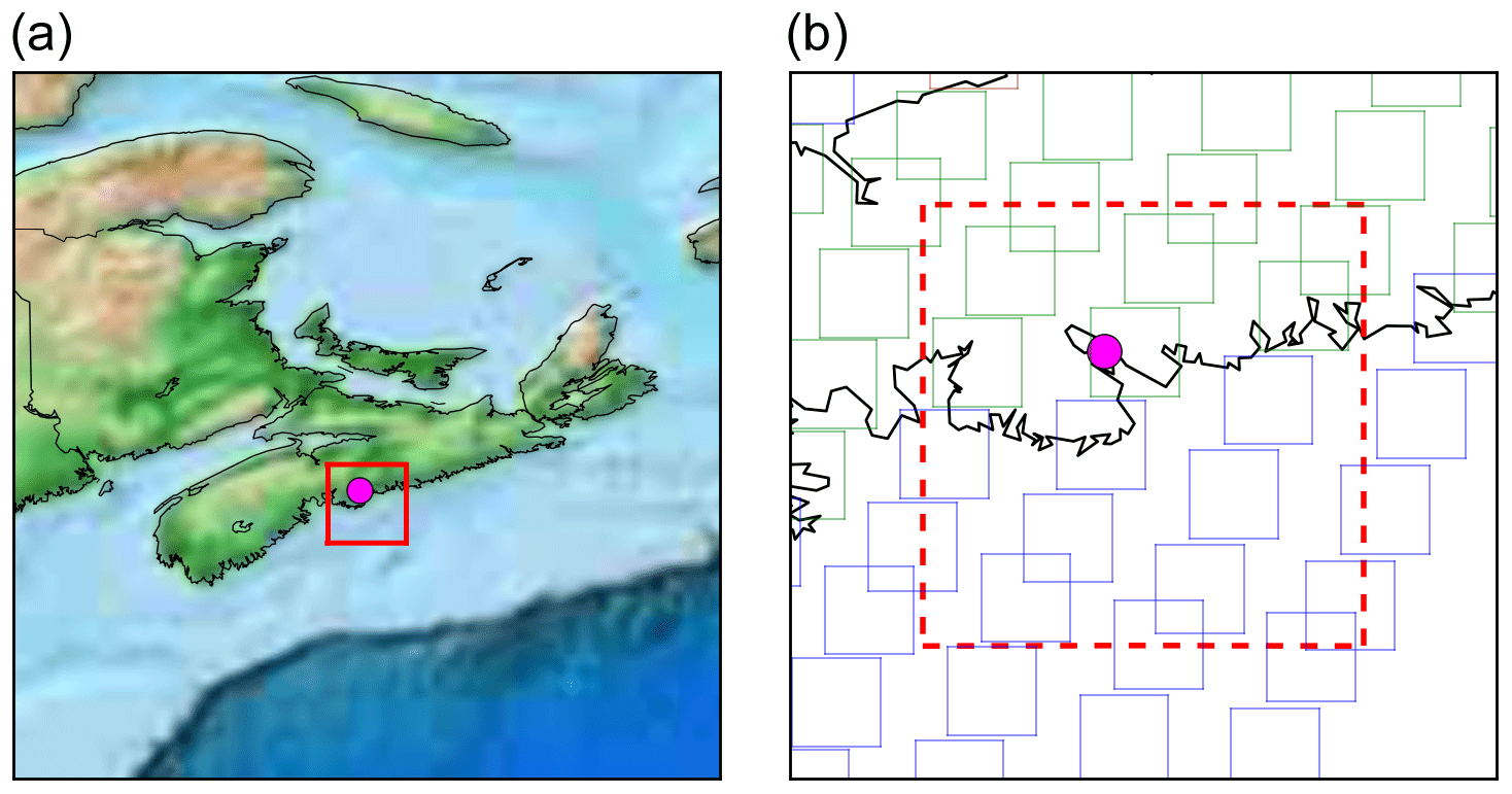
Figure 1(a) Map of Nova Scotia and the surrounding region in Atlantic Canada. Lighter colours on land indicate higher elevation. The pink dot shows the location of Halifax, the coastal city that we focus on in this study (see Sect. 2.1.3), and the red box shows the MOPITT L3 grid box containing Halifax. (b) Map zoomed to the MOPITT L3 grid box containing Halifax (red dashed box), with the approximate location of individual L2 retrieval footprints shown (blue boxes represent the L2 surface index of water; green boxes represent the L2 surface index of land). L2 retrieval footprints with a midpoint that falls within the boundaries of the L3 grid box will be averaged together to create the L3 data, according to certain rules – see Sect. 2.1.2 for full explanation.
This paper is structured as follows: in Sect. 2 we outline the data and methods used in this study, giving an overview of the MOPITT instrument, retrieval, and surface type classification that is relevant to our work. In Sect. 3 our results are presented and discussed, and conclusions are drawn in Sect. 4.
2.1 MOPITT
2.1.1 Instrument and retrieval overview
MOPITT has been making routine observations almost continuously since March 2000. It is carried on board the polar-orbiting NASA Terra satellite, with a nominal altitude of ∼705 km and an equatorial overpass time of ∼ 10:30 and ∼ 22:30 local time. The instrument is a nadir-viewing gas correlation radiometer, with a ground resolution of 22 km×22 km. It observes radiances in two CO-sensitive spectral bands: the TIR at 4.7 µm and the NIR at 2.3 µm. The TIR band is sensitive to both absorption and emission by CO and yields information on its vertical distribution in the troposphere (Pan et al., 1995, 1998). The NIR band measures reflected solar radiation, which constrains the CO total column amount and yields information on CO concentrations in the lower troposphere (LT), to which TIR radiances are typically less sensitive (Pan et al., 1995, 1998). NIR radiances can, however, only be exploited in daytime scenes over land. Our results are based on analysis of the TIR–NIR combined product, owing to its greater sensitivity to LT CO compared to the TIR- and NIR-only products which are also available (e.g. Deeter et al., 2017). Owing to the increased LT sensitivity from NIR radiances being limited to retrievals over land, we expect that the results presented here show an upper bound on (i) the retrieval differences between surface types within our coastal L3 grid box of focus and (ii) the consequent effects on sample statistics and temporal trends that we outline. Differences are still found in the TIR-only product, however, and we outline these in Sect. S1 in the Supplement. We restrict our analysis to daytime-only retrievals (more information on data selection in Sect. 2.1.3).
Multiple other sources describe MOPITT's CO retrieval algorithm in detail (e.g. Deeter et al., 2003; Francis et al., 2017). Briefly, it employs optimal estimation (Pan et al., 1998; Rogers, 2000) and a fast radiative transfer model (Edwards et al., 1999) to invert radiance measurements performed by the instrument to obtain CO concentrations. Additional inputs required include meteorological data (profiles of temperature and water vapour), surface temperature and emissivity, and satellite viewing geometry for the radiative transfer model, as well as a priori CO profiles to constrain the inversion to physically reasonable limits. For latest MOPITT product versions, meteorological fields are extracted from the NASA Modern-Era Retrospective Analysis for Research and Applications Version 2 (MERRA-2) reanalysis product; and a priori CO profiles are derived from a monthly CO climatology for the years 2000–2009, simulated with the Community Atmosphere Model with Chemistry (CAM-chem) chemical transport model at a spatial resolution of (Lamarque et al., 2012) and then spatially and temporally interpolated to the time and location of the MOPITT observation. As it is a multi-year climatology, the a priori features no yearly trend; i.e. values for a given location and day of the year are the same every year. Surface temperature and emissivity values are retrieved from the radiance measurements (the retrieval also requires a priori information for these measurements). Retrievals are only performed for cloud-free scenes, with cloud screening based on collocated Moderate Resolution Imaging Spectroradiometer (MODIS) observations and MOPITT's own radiances. CO profiles are retrieved on 10 vertical levels, with 9 equally spaced pressure levels from 900 to 100 hPa (the uppermost level covers the atmospheric layer from 100 to 50 hPa) and a floating surface pressure level. Where the surface pressure is below 900 hPa, less than 10 profile levels are retrieved. Reported values represent the mean CO volume mixing ratio (VMR) in the layer immediately above that level. Retrievals are initially performed on a log 10(VMR) scale, owing to large CO variability in the atmosphere.
Averaging kernels are produced for each retrieval and distributed with the data. The AK matrix (A) quantifies the sensitivity of the retrieved vertical profile to the true vertical profile and depends on the radiance weighting functions, instrument error covariance matrix, and a priori covariance matrix. Its relationship to the retrieved profile (Xrtv), the true profile (Xtrue), and the a priori profile (Xapr) is expressed as follows (e.g. Deeter et al., 2017):
Thorough analysis of AKs is essential for understanding the physical significance of MOPITT's CO retrievals. We discuss AKs in more detail in Sect. 3.1.2.
The MOPITT retrieval algorithm is subject to continuous development, in line with improvements in understanding of the changing instrumental characteristics and geophysical factors that affect the retrieval sensitivity, and with periodic updates to the radiative transfer model (Worden et al., 2014). This prompts the release of new product versions, with enhanced validation statistics against in situ CO observations. The work presented in this paper is based on MOPITT Version 7 (V7) products (Deeter et al., 2017). We analyse both L2 and L3 products (as outlined below). It should be noted that MOPITT Version 8 products have been released very recently, incorporating an improved radiance bias correction method to address a documented drift and geographical variability in retrieval bias compared to in situ measurements (Deeter et al., 2019). It remains to be seen whether the impacts of land–water retrieval sensitivity contrasts documented in this study remain in this newest product version.
2.1.2 Surface type classification
Both L2 and L3 data files come with a range of diagnostic fields and values, in addition to the averaging kernel matrix, that can be used for filtering and interpreting retrievals. Of particular importance is the surface index flag. Because retrieval information content is variable depending on surface type (Deeter et al., 2007), each L2 retrieval is tagged according to whether it was performed over land, water, or a combination of the two (mixed). The surface index of each L3 grid box is then based on the L2 retrievals that fall within the relevant grid boundaries (Fig. 1). Where more than 75 % of the bounded L2 retrievals have the same surface index, only those retrievals are used to produce the L3 gridded value (the other L2 retrievals are discarded), and the L3 surface index is set to that surface type. Otherwise, all L2 retrievals available in the L3 grid box are averaged together and the L3 surface index is set to mixed (this information is taken from the MOPITT Version 6 L3 data quality summary1 – at the time of writing, no V7 L3 data quality summary was available).
The averaging together of retrievals with significantly different sensitivity profiles – as could be the case when averaging retrievals over land and water – serves to dilute the information coming from the MOPITT observed radiances with information coming from the a priori, thus increasing the dependence of the resulting CO profile values on the a priori profile. In fact, guidelines to maximize the information content of MOPITT data and minimize the influence of the a priori are to restrict analysis to daytime observations over land during the summer season, since this is when thermal contrast conditions are greatest, thus maximizing the instrument's ability to sense CO in the lowermost layers of the troposphere (MOPITT Algorithm Development Team, 2017; Deeter et al., 2015, 2007). Unfortunately, such filtering does lead to an overall loss of available retrievals for analysis, reducing the effective temporal and spatial coverage of the data.
2.1.3 Study area, time period, and MOPITT data processing in this study
Our analysis is based on MOPITT retrievals over the city of Halifax in Nova Scotia, Canada (Fig. 1: longitude −63.58∘, latitude 44.65∘). Situated on the Atlantic coastline, Halifax is the major economic centre in Atlantic Canada, with a population in excess of 315 000 in the urban core of Halifax Harbour (from 2016 census statistics). The pollution environment of Halifax, which is an intermediate port city, was characterized in detail by Wiacek et al. (2018 – trace gases of focus include SOx, CO2, CO, NOx, O3, HC, and PM); briefly, it showed no exceedances of regulated gaseous contaminants, but nevertheless a substantial contribution of shipping emissions that is comparable to or greater than emissions from the city's vehicle fleet and a nearby 500 MW power plant. All available MOPITT V7 L2 and L3 TIR–NIR files (MOP02J and MOP03J files, respectively) were downloaded from the NASA Earthdata portal (https://search.earthdata.nasa.gov, last access: 11 June 2020). There is a small inconsistency in the data record before and after an instrumental reconfiguration in 2001 (Drummond et al., 2010); we therefore discard all data prior to this reconfiguration. The remaining data covers the period 25 August 2001 to 5 March 2017. At the time of writing, more recent data are flagged as beta files, which await a future retrospective processing after the annual hot calibration becomes available, and their use in scientific analyses is discouraged (Deeter et al., 2017). For clarity and brevity, we restrict our main analyses and discussion to the winter (DJF) and summer (JJA) seasons, since these best encapsulate the different thermal contrast conditions over land and water, when compared to the intermediate (MAM and SON) seasons. For completeness, we demonstrate that our findings also hold for MAM and SON in Sect. 3.3.
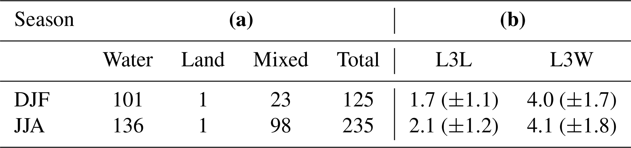
We extract L3 data for the grid box that contains the city of Halifax, and retain only the observations that were made during daytime hours. This yields a time series with one observation per day, when retrieval data were available within this grid box. There are no retrievals available on 91 % of all days in DJF and 83 % of all days in JJA for the period covered. This is a result of both (1) MOPITT's polar orbit limiting temporal resolution to ∼3 d over most of the globe; and (2) on days when the satellite's swath does encompass Halifax, retrievals either not being made due to cloud coverage, or discarded due to data quality issues. While this does not prevent a meaningful comparison of available retrievals, it does mean that caution is needed when using them to draw conclusions about the time period covered as a whole, which is something that we do not attempt to do. For clarity, we refer to the original, as-downloaded L3 time series as L3O for the remainder of this paper, owing to the way that we process the L2 data (explained below). Because this grid box straddles the coastline, the L3O surface index varies each day. The surface classification breakdown of the L3O time series is given in Table 1a. “Water” is the modal classification in both seasons, followed by “mixed”. L3O is only classified as “land” on one occasion each season. This is most likely due to the fact that more of the L3 grid box is situated over water than land (Fig. 1). The ratio of water to mixed observations is far greater in DJF than in JJA. This may be due to preferential cloud coverage over land in winter and/or could be linked to the misidentification of snow/ice coverage on the surface as cloud during cloud screening (identifying the exact cause for this difference is beyond the scope of this paper).
Table 1(a) Surface classification of L3 data for the grid box containing Halifax (L3O) for the period 25 August 2001 to 5 March 2017. Note that no retrievals are available for this L3 grid box on 91 % of days in DJF and 83 % of days in JJA. (b) Mean number of individual L2 retrievals with land and water surface index that contribute to the L3L and L3W time series, respectively (the standard deviation is in brackets).
We select all L2 retrievals that fall within the L3 grid box that contains the city of Halifax (lower-left corner: −64∘ E, 44∘ N; upper-right corner: −63∘ E, 45∘ N). Because we directly compare the L2 retrievals to the L3 product that they create, we filter these based on pixel number (each pixel corresponds to one of MOPITT's four along-track detectors) and channel-average signal-to-noise ratio (SNR), as is done at the V7 L3 processing stage to improve L3 information content by excluding observations from specific detector elements on MOPITT's detector array that were found to exhibit greater retrieval noise than the other elements (MOPITT Algorithm Development Team, 2017; Deeter et al., 2017). Specifically, these filters exclude the following: all observations for pixel 3 and all observations where both (1) the channel 5A SNR <1000 and (2) the channel 6A SNR <400. Channels 5A and 6A correspond to the average radiances for MOPITT's length-modulated cell TIR and NIR channels, respectively. Finally, we only retain daytime retrievals, using a solar zenith angle filter of <80∘.
From this subset of L2 retrievals, we take separate area averages for those with a surface index of land and water, creating two time series that are effectively new L3 land-only and water-only products, for days when MOPITT retrievals over Halifax are available. We herein refer to these as L3L and L3W, respectively. For clarity of analysis, we discard remaining L2 retrievals with a surface index of mixed (these account for ∼5 % of the total L2 retrieval subset). The number of individual L2 retrievals that are averaged together each day to create L3L and L3W is given in Table 1b. From this, it is clear that there are around double the number of L2 retrievals over water than land within the L3 grid box containing Halifax, which explains the dominance of water in the L3O surface classification (Table 1a) and also means that L2 retrievals over water will have a greater weighting in L3O than L2 retrievals over land on days when the surface index is mixed.
2.2 Retrieval simulation
To demonstrate how MOPITT retrieved CO concentrations are affected by retrieval sensitivity (Sect. 3.1.3), we simulate pairs of L3L and L3W retrieved profiles that are obtained concurrently (i.e. retrieved on the same day – on some days, one of L3L or L3W is missing) as follows:
For each simulated retrieval, Xtr, sim is taken from the Copernicus Atmospheric Monitoring Service (CAMS) reanalysis (CAMSRA – see Sect. 2.3), for the model grid box that contains Halifax, for the corresponding month and year of the observed retrieval (because the CAMSRA data are monthly mean values); Xapr, sim is the mean of the a priori fields that correspond to the temporally coincident L3L and L3W pairings; and A is the retrieval averaging kernel from L3L or L3W. Thus, any differences between each pair of simulated retrievals (Xsim, L3L and Xsim, L3W) are solely a result of differences in A, since Xtr, sim and Xapr, sim are identical for both. Simulations are initially performed on log 10(VMR) for consistency with the MOPITT retrieval algorithm and then converted back to VMR scale for analysis.
2.3 Additional datasets
The CAMSRA dataset to simulate retrievals is described by Inness et al. (2019). For the CAMSRA grid box containing Halifax (horizontal resolution is ), we extract CO volume mixing ratios for levels 1000–100 hPa at 100 hPa intervals, which correspond to the MOPITT levels of the profile. The CAMSRA dataset has no surface level, so we take the 1000 hPa level (the lowest level available in the dataset) to correspond to MOPITT's floating surface level. At the time of writing, CAMSRA data are only available for the years 2003–2016.
Information on mean wind patterns across Nova Scotia and the surrounding area is taken from the European Centre For Medium-Range Weather Forecasts (ECMWF) ERA-Interim dataset (horizontal resolution is ; see Dee et al., 2011, for a dataset overview). We analyse daily mean u and v vector winds for the following levels: 10 m (the closest level to the surface for winds in the dataset) and 850 and 500 hPa (which correspond roughly to the lower- and mid- troposphere, respectively). In addition, we extract monthly mean temperature profile data (at 100 hPa intervals, plus the skin temperature and 2 m air temperature variables) for the closest model grid boxes to Halifax that exclusively cover land and ocean, in order to illustrate the typical land-only and water-only temperature profiles that correspond to the MOPITT L2 retrievals over land and water that are analysed.
3.1 Impact of retrieval sensitivity differences on temporally coincident L3L and L3W retrievals
In this section we compare the L3L and L3W CO retrievals and demonstrate where and when there are differences in retrieved CO concentrations that are clearly linked to differences in retrieval sensitivity over land and water. We restrict our analysis to days when the L3O surface index is mixed and both L3L and L3W retrievals are present, in order to minimize any potential differences in the true profile between land and water (there are a couple of days in the L3O time series when one or the other of L3L or L3W is missing, even when the L3O surface index is mixed, owing to the presence of L2 retrievals with a surface index of mixed, which we have discarded). Thus, an underlying assumption here is that land–water differences in the true profile for retrievals contributing to L3L and L3W are small, owing to the fact that they are retrieved in close spatial proximity to each other (i.e. within the same grid box) and at the same time. We test this assumption in Sect. 3.1.4 and 3.1.5.
3.1.1 Climatology of land–water retrieval and a priori differences
Figure 2 shows the percentage difference between temporally coincident retrieved VMRs for selected levels of the profile and for CO total column (TCO) amounts (ΔRET) in L3L and L3W. Positive (negative) differences indicate that retrieved VMRs/TCO are greater (less) in L3W than L3L. Differences are expressed as percent values, rather than differences in measurements units, so that we can display profile and TCO retrievals on the same plot (profile units are ppbv, and TCO units are molecules cm−2).
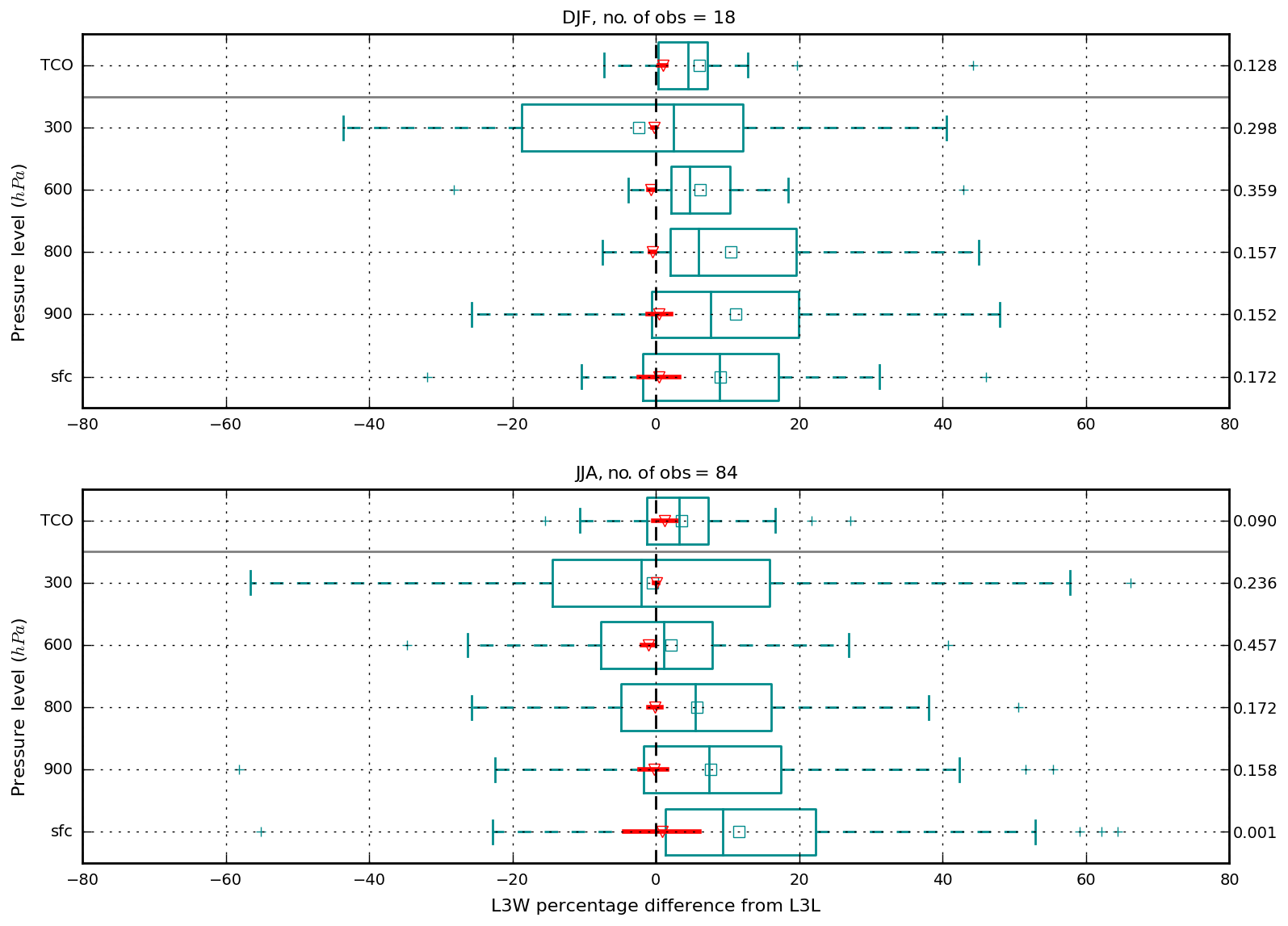
Figure 2Distribution of percentage difference (method for calculating percentage differences: ) between temporally coincident retrieved VMRs (selected profile levels) and CO total column (TCO) from L3W and L3L. Squares represent mean differences, with the p value associated with each mean difference (from a two-tailed Student t test) given on the right-hand-side y axis. Plus symbols represent outliers (outliers defined as above (below) percentile ). Red triangles represent the mean percentage difference between a priori values. Red lines represent the range of a priori difference values (where barely visible this means range is very small).
In both seasons, mean retrieved VMRs are greater in L3W than L3L in the lower troposphere (LT – surface, 900 and 800 hPa levels), with a maximum mean difference of 11.6 % (14.3 ppbv) at the surface level in JJA, the only profile location where the mean difference is significant (p=0.001). The spread of ΔRET values is comparable in both seasons at these levels, with a clear skew towards positive values. Thus, although retrieved LT VMRs in L3L may occasionally exceed those in L3W by over 20 %, they are usually greater over water than land. Mean ΔRET values are closer to zero and less significant in the MT and UT (represented by the 600 and 300 hPa profile levels respectively), indicating that differences in retrieved VMRs are not as persistent at higher altitudes. However, the spread in ΔRET remains large at these altitudes, with retrieved VMRs in L3L and L3W differing by over ±40 % on individual days (with outliers exceeding ±60 %). TCO is greater in L3W than L3L in both seasons, significantly so in JJA. This is consistent with the most persistent VMR differences occurring in the LT, where atmospheric densities are greatest, thus contributing a relatively greater amount to the total column than MT and UT levels.
Our assumption in this section is that L2 retrieved CO concentrations obtained within the same L3 grid box should be similar. We may actually expect retrieved CO amounts in L3L to be greater than those in L3W due to CO sources existing on land, particularly within the city of Halifax. One reason for the ΔRET values instead indicating higher concentrations over water could be differences in the a priori profiles (ΔAPR) used in the corresponding retrievals. The L2 retrievals over land and water have different a priori profiles owing to spatial interpolation of the model climatology to the 22 km×22 km footprint of the MOPITT L2 retrieval. However, as Fig. 2 demonstrates, ΔAPR values are small in comparison to ΔRET, with mean difference values very close to zero and a maximum range of 10.4 % (occurring at the surface level in JJA). Moreover, the sign of mean ΔAPR does not match that of mean ΔRET at several levels in both seasons (i.e. retrieved VMRs in L3W are greater than in L3L, but a priori VMRs are less). It therefore appears unlikely that a priori profile differences are responsible for the observed differences in retrieved CO concentrations in L3L and L3W.
3.1.2 Climatology of land–water retrieval sensitivity differences
An alternative explanation for the observed ΔRET could be differences in retrieval sensitivity over land and water, quantified by the retrieval AK matrix. Figure 3 compares the mean AKs corresponding to the retrieved profiles in L3L and L3W analysed in the previous section. Each curve corresponds to a row of the AK matrix and represents the sensitivity of the corresponding level of the retrieved profile to each level of the true CO profile, with the widest part of each AK in the x direction (when a peak is evident) indicating the portion of the true profile that the corresponding level of the retrieved profile is most sensitive to. The sum of the elements in each AK row represents the overall sensitivity of the retrieved profile at the corresponding pressure level to the whole true profile; values close to zero indicate that the retrieval is relatively insensitive to the true profile and therefore closely tied to the a priori profile, while the converse is true as the rowsum approaches one. The mathematical trace of the AK matrix (i.e. sum of the diagonals) gives the degrees of freedom for signal (DFS) of the retrieval, which is a measure of the number of independent pieces of information (in other words, information content) in the retrieval from the measurement, with respect to the true profile. When DFS values approach two, this is interpreted as the retrieval being able to resolve CO in two independent atmospheric layers.
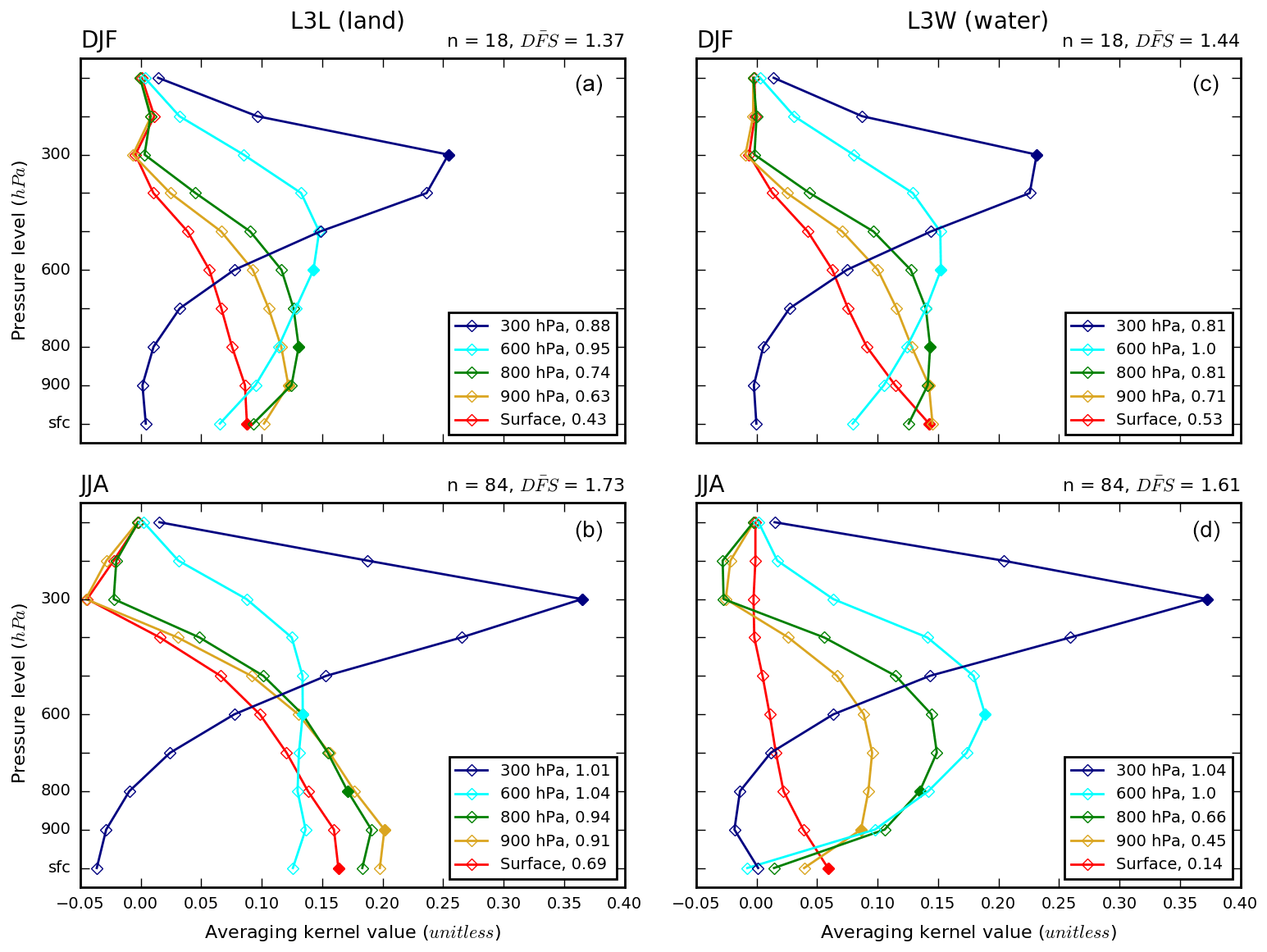
Figure 3Mean retrieval averaging kernel (AK) rows and DFS values for L3L (land, a, b) and L3W (water, c, d) in DJF (a, c) and JJA (b, d), for selected profile levels only. Filled diamonds indicate the diagonal value location for that AK. Numbers in legend indicate the corresponding retrieval level of AK and show the mean rowsum for that AK level.
There are some clear differences between the mean AKs over land (from L3L) and water (from L3W) shown in Fig. 3. In DJF, AKs for LT (especially surface level) retrievals reach greater values in the LT in L3W than L3L, indicating that sensitivity to the true profile at these levels is actually greater in L3W (surface level AK peak is 0.14 for water and 0.09 for land, both at the surface level). This is reflected in greater rowsum values for LT AKs in L3W than L3L. Differences in MT (600 hPa) and UT (300 hPa) AKs are much less pronounced, with sensitivity to the true profile actually becoming slightly greater in L3L than L3W higher up in the troposphere. In JJA, the mean LT and MT AKs are qualitatively much more different between L3L and L3W than in DJF. LT rowsums are significantly greater in L3L (p<0.001 at the surface, 900 and 800 hPa profile levels; see Sect. S2) and closer to one, signifying that these retrievals contain much more true profile information than those in L3W. The AK shapes also indicate that the respective retrievals are sensitive to different parts of the true profile. In L3L, surface and LT AKs peak at either the surface (surface level AK) or at 900 hPa (both the 900 and 800 hPa level AKs) and decline towards the UT, while MT AKs indicate relatively equal sensitivity throughout the LT, MT and the lower levels of the UT. In L3W on the other hand, LT and MT AKs (excluding the largely insensitive surface level) indicate relatively little sensitivity in the lowest profile levels and peak in the MT. The surface level AK in L3W actually indicates close to zero sensitivity throughout the profile, aside from a very weak peak at the surface level, which is around 3 times lower than that over land. As in DJF, UT AKs are quite similar, except for relatively small differences at the surface, where the 300 hPa AK over land actually indicates negative sensitivity. Differences in mean DFS values for retrievals in L3L and L3W are greater in JJA (−0.12) than DJF (0.07), highlighting the greater land–water sensitivity contrast in JJA and also reflecting the switch in surface type exhibiting the greatest LT retrieval sensitivity between the seasons.
The differences in surface and LT AKs for MOPITT retrievals in L3L and L3W discussed above can be accounted for primarily by the differing LT thermal contrast conditions over land and water, as explored in detail by Deeter et al. (2007). The sensitivity of MOPITT retrievals to CO in the LT is predominantly controlled by the thermal contrast between the surface skin temperature (Tskin) and the surface air temperature (Tsfc), as well as by the tropospheric temperature profile. Seasonal mean temperature profile data from ERA-Interim for the nearest land-only and water-only model grid boxes to Halifax show clear differences in DJF and JJA (Fig. 4). In DJF, Tskin is around 6 ∘K warmer than the 2 m air temperature (T2 m, which we use as a proxy for Tsfc as this is the lowest model level) over water and a further degree warmer than the air at 1000 hPa, whereas the temperature gradient is weak/slightly inverted over land, with Tskin less than a degree warmer than T2 m, which is actually slightly cooler than the air at 1000 hPa. Correspondingly, the lowest couple of retrieval levels indicate greater sensitivity to the surface and LT over water (in L3W) than land (in L3L) in DJF (Fig. 3). Temperature profiles converge towards the MT, as do AKs. In JJA on the other hand, there is a clear gradient between Tskin and the overlying air on land, while the ocean surface is actually cooler than the air above, up to a height of 900 hPa. As a result, surface and LT sensitivity is greater in L3L than in L3W in JJA, with the sensitivity of retrievals in L3W approaching zero close to the surface owing to this inverted temperature profile. The Tskin increase approaching 20 K between DJF and JJA likely also accounts for the relatively greater overall true profile sensitivity (indicated by DFS values) in JJA for L3L than in DJF for L3W. Since our analysis is conducted using the joint TIR–NIR product, it is important to bear in mind that the benefit of enhanced LT sensitivity due to the incorporation of NIR is limited to retrievals over land, so this will also have an impact on the AK differences presented above. However, a land–water retrieval sensitivity contrast of comparable magnitude to that presented here is also evident in the TIR-only product, reinforcing the primary role of thermal contrast differences (see Sect. S1).
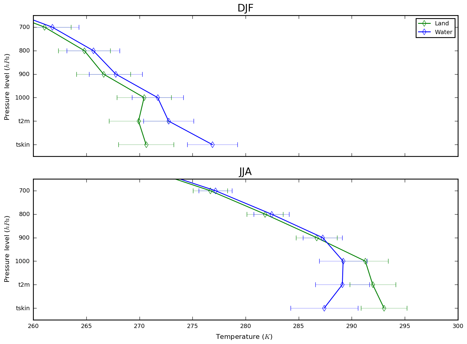
Figure 4Mean temperature profile from ERA-Interim for the closest all-land and all-water model grid boxes to Halifax. Error bars show the standard deviation. Data are the mean of the 12:00 and 18:00 UTC time steps (this corresponds to 08:00 and 14:00 local time, the closest ERA-Interim time steps to the local MOPITT overpass time of ∼ 10:30) for 2001–2017.
That the retrieval sensitivity contrast between L3L and L3W is most pronounced in the LT is consistent with the finding that retrieved CO profiles in L3L and L3W show the greatest differences in the LT. Although mean retrieval sensitivity in L3L and L3W converges with altitude, differences do exist from day to day, but they are neither as large nor as skewed in favour of retrievals over land or water (depending on season) as in the LT (see Sect. S2), where there is a well-understood thermal contrast mechanism creating the systematic land–water sensitivity contrast. Likely causes for this could be day-to-day changes in atmospheric conditions (i.e. temperature or water vapour profiles), or random instrumental or retrieval noise.
3.1.3 Control of ΔRET by land–water sensitivity differences
To demonstrate that retrieval sensitivity differences over land and water can lead to the observed differences between CO profiles in L3L and L3W that are retrieved at the same time, we simulate and compare the pairs of retrieved CO profiles in L3L and L3W that are analysed in the preceding sections, using the transformation outlined in Sect. 2.2. Recall that any differences between each pair of simulated retrievals are solely a result of differences in AKs. Because available CAMSRA data only cover the years 2003–2016, only a subset of the retrieval pairings considered in earlier sections (which span the period 2001–2017) are simulated.
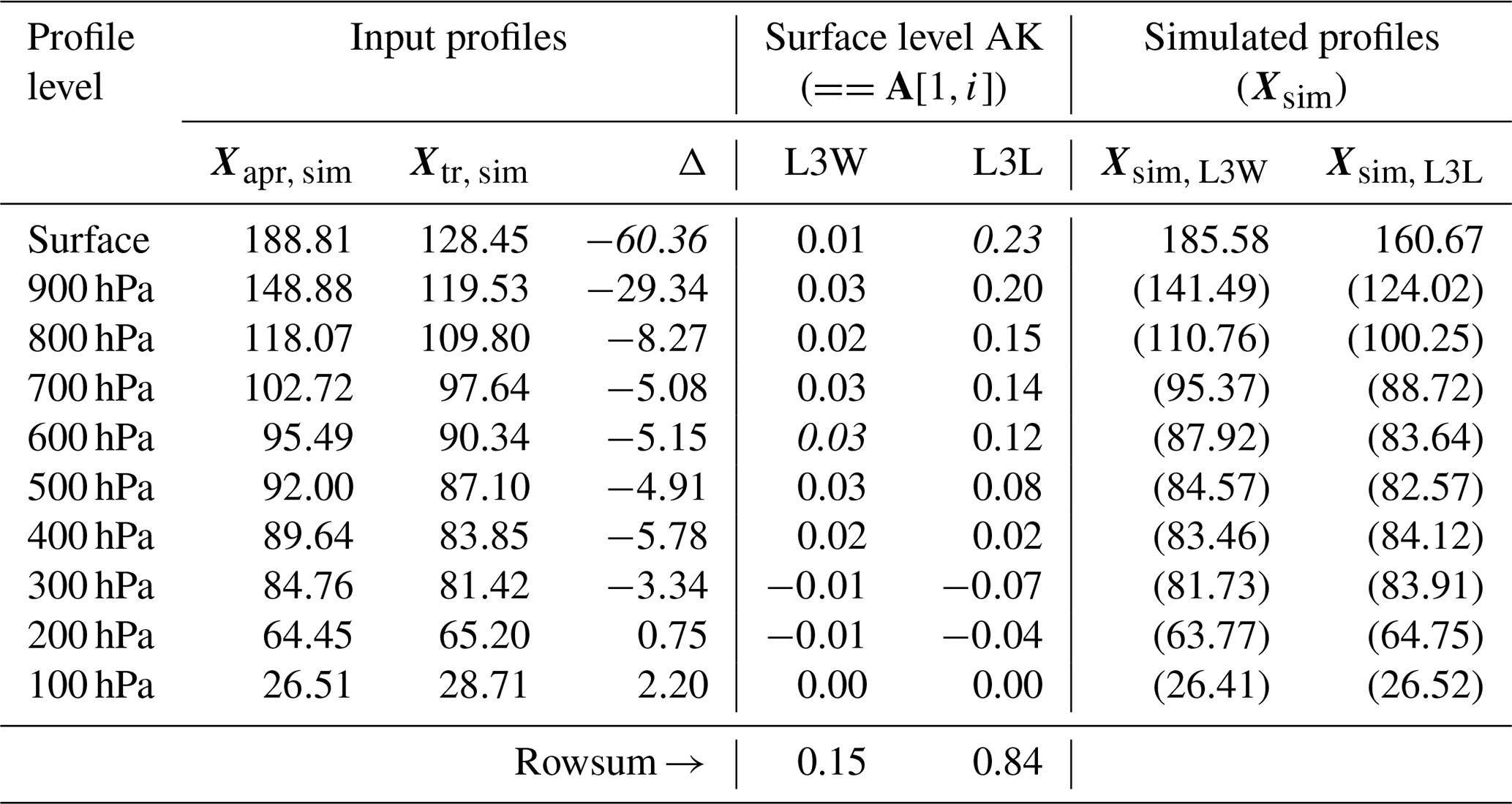
We first demonstrate the sensitivity effect with a case study on 18 August 2013. Profiles (a priori (Xapr, sim) and truth (Xtr, sim)) and surface level AKs used in the simulation, and the resulting Xsim, L3L and Xsim, L3W, are given in Table 2. For brevity, we only focus on the surface level. In this example, Xtr, sim is considerably lower than Xapr, sim at the surface level, and several features of the AKs indicate greater sensitivity to Xtr, sim in L3L and L3W: the AK value is significantly greater at the surface in L3L than L3W, and the rowsum is over 5 times as high. Correspondingly, Xsim, L3L is much lower than Xsim, L3W at the surface and much closer to Xtr, sim (32.21 ppbv higher vs. 57.13 ppbv higher). Both Xsim, L3L and Xsim, L3W indicate that Xtr, sim is lower than Xapr, sim at the surface, but Xsim, L3L gives the closer estimate, as would be expected. In both cases, a portion of the overall departure from Xapr, sim at the surface level (in other words, value added over the a priori) originates at other levels of the profile and not the surface level itself. This is a result of the surface level AK being nonzero at other levels and is a function of the inter-level correlation of the original retrieval, which is linked to the a priori covariance matrix used in the retrieval (Deeter et al., 2010).
Table 2Case study information for simulated L3L and L3W profile retrievals (Xsim, L3L and Xsim, L3W respectively) for 18 August 2013. . Values that are italicized indicate the maxima (by magnitude) for that column. Simulated profile values for levels 900–100 hPa are shown in brackets because AKs and calculations for these levels are not discussed in the text and AKs for the 900–100 hPa levels are not shown.
We now consider differences between all Xsim, L3W and Xsim, L3L pairings (ΔSIM) throughout the profile and compare these to the observed differences between temporally coincident retrievals in L3L and L3W (ΔRET) discussed previously (Fig. 5a). For ease of comparison, ΔRET values are overlaid (faint lines) for the shorter time period matching CAMSRA data availability (the 2003–2016 ΔRET patterns are very similar to those seen in Fig. 2). It should be noted that we cannot expect ΔSIM to match ΔRET exactly, owing to (possibly large) differences between the Xtr, sim profiles used in the simulations and the (unknown) true profiles at the time of the actual MOPITT retrievals (Xtrue). For instance, Xtr, sim is a monthly mean value from a reanalysis model, whereas Xtrue varies by day, which should result in less variance in ΔSIM than ΔRET. In DJF, mean ΔSIM is negligible at all profile levels shown, and the range of values is far smaller than seen for ΔRET. In JJA on the other hand, ΔSIM reaches considerably larger values than in DJF, and mean values are significantly different (p<0.05) over land and water at all but one level shown (300 hPa). LT and MT ΔSIM distributions are a remarkably good match for ΔRET, given the likely substantial differences between Xtr, sim and Xtrue. In the UT, ΔSIM values are somewhat smaller, although this is not unexpected given the smaller land–water AK differences evident in Fig. 3.
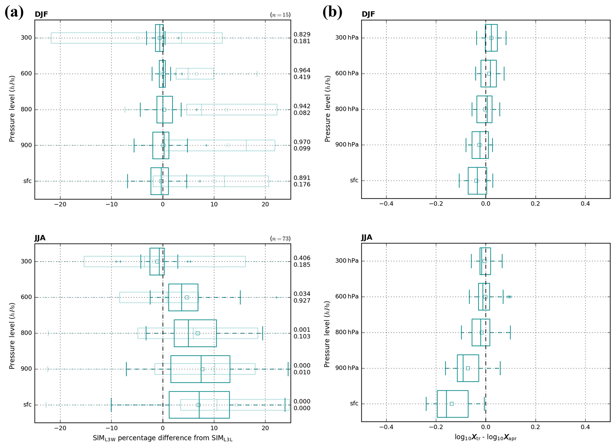
Figure 5(a) Distribution of percentage difference (method for calculating percentage differences: ) between simulated temporally coincident VMR retrievals in L3W (SIML3W) and L3L (SIML3L). Squares represent mean differences. The p value associated with each mean difference (from a two-tailed Student t test) is given on the right-hand-side y axis (top value shows ΔSIM; bottom value shows ΔRET). Plus symbols represent outliers (outliers defined as above (below) percentile ). Faint shading shows the corresponding ΔRET boxplots for comparison. Note that the sample size is different to Fig. 2 owing to the CAMSRA data used as the Xtr, sim profile only covering a subset of the MOPITT years (2003–2016 vs. 2001–2017 in Fig. 2). The ΔRET boxplots overlaid cover this shortened period. (b) Distribution of the values calculated during the simulation of retrieved profiles (see Eq. 2) in DJF (top subpanel) and JJA (bottom subpanel).
That L3L and L3W simulated and retrieved profile differences over land and water are comparable in JJA is clear evidence that ΔRET is strongly influenced by the land–water sensitivity contrast in summer months, at least in the LT. However, while ΔSIM values are of a much smaller magnitude in DJF than in JJA, ΔRET is actually of a similar magnitude in both seasons. The question therefore arises as to why ΔSIM is so different from ΔRET in DJF and why it is of much smaller magnitude in DJF than JJA. Considering the terms of Eq. (2), there are two possible explanations. Firstly, differences between L3L and L3W LT and MT AKs (A in Eq. 2) are much smaller in DJF than in JJA (Fig. 3). This means that the deviation of Xsim, L3W and Xsim, L3L from Xapr, sim will be more similar in DJF (resulting in small ΔSIM), as opposed to in JJA, where as was seen in the case study discussed above, Xsim, L3L can deviate more from Xapr, sim than Xsim, L3W owing to increased sensitivity in L3L in the lower profile levels (resulting in greater ΔSIM than in DJF). In the UT, AK differences are comparable in both seasons, and ΔSIM is correspondingly similar. Secondly, the magnitude of from Eq. (2) is, on average, around 4 (3) times greater in JJA than in DJF at the surface (900 hPa) level (Fig. 5b). Xsim, L3L therefore deviates more from Xapr, sim than Xsim, L3W throughout the LT and MT in JJA owing to strong contrasts in near-surface sensitivity at these profile levels, thus yielding large ΔSIM. Conversely, closer Xtr, sim and Xapr, sim profiles combine with small sensitivity differences to limit ΔSIM in DJF. A final, alternative explanation for ΔSIM being a poor match for ΔRET in DJF, unlike in JJA, is that sensitivity differences in L3L and L3W could have less of an impact on ΔRET in DJF than in JJA and that something else is responsible – for example, real differences between the true CO profile over land and water. This is something we explore in detail in the following sections.
3.1.4 Regional land–water contrast in L2 data
To further evaluate whether ΔRET within the L3 grid box containing Halifax is a function of land–water sensitivity contrasts or actually due to real gradients in the true CO profile (for example, due to offshore transport of emissions from the city of Halifax or marine–land chemistry differences), we analyse the characteristics of retrieved profiles over the broader geographical region surrounding Halifax. If ΔRET is linked to sensitivity, then we would expect there to be a clear land–sea contrast across the whole region. This is exactly what we see. Figure 6 shows seasonal median L2 retrieved and a priori CO concentrations for the surface level of the profile, where ΔRET and L3L–L3W AK differences are greatest and most significant, for the Canadian maritime provinces and a small portion of the northeastern United States (note that we show seasonal median fields here as the spatial patterns are clearer than for plots consisting only of the subset of days analysed in the rest of this section. The corresponding plot for the subset of days is shown in Sect. S3, and the main findings are unchanged). Difference fields (RET–APR) are also shown. In JJA, a land–sea contrast is remarkably clear in both the retrieved and RET–APR fields. The a priori field shows elevated CO amounts emanating from the west-southwest (indicative of CO sources in the northeastern United States and around the Great Lakes) and decreasing quite smoothly towards the north and east. The west-southwest maxima is replicated in the retrieved field, but the smoothly decreasing gradient is clearly broken, with the land in the image characterized by lower CO values than the adjacent ocean. This contrast is enhanced further in the RET–APR field. RET–APR values close to zero indicate either very low retrieval sensitivity or closely matching retrieved and a priori values. The analysis of averaging kernels in Sect. 3.1.2 demonstrated the lack of retrieval sensitivity at the surface over water (in L3W) in JJA. On average, the RET–APR field is 11.5 ppbv lower over land than over water (determined by binning the L2 data for the region shown according to surface classification). This reinforces our earlier interpretation that, in JJA, LT retrievals in L3W are weighted more heavily towards an a priori profile in which CO concentrations are too high than LT retrievals in L3L.
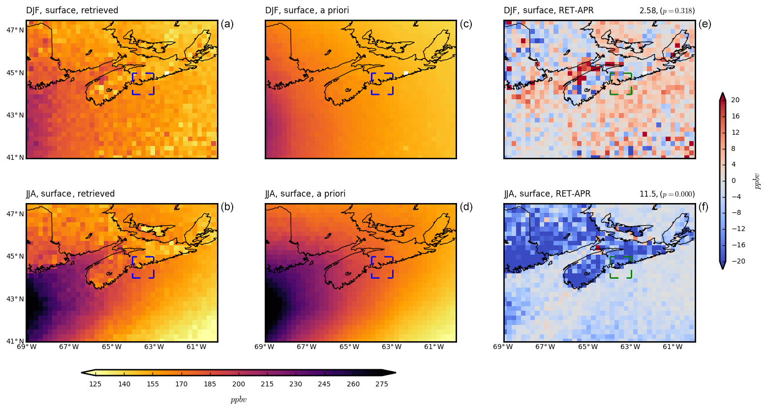
Figure 6Seasonal median L2 (these maps were created from L2 data that were interpolated to a regular grid for ease of plotting.) retrieved VMR (a, b), a priori VMR (c, d), and RET–APR (e, f) at the surface profile level in DJF (a, c, e) and JJA (b, d, f). Values to the right above RET–APR plots equal for plotted area (data were first binned according to L2 surface index); numbers in brackets correspond to significance of mean difference using a two-tailed Student t test. Blue or green dashed squares represent the outline of the L3 grid box that contains Halifax.
The land–sea contrast is less clear in DJF, although the RET–APR field does indicate generally positive values over water and negative values over land. The contrast being less apparent in DJF compared to JJA is consistent with the smaller L3L–L3W AK differences in DJF compared to JJA. However, it is surprising that RET–APR changes sign from land (generally negative) to water (generally positive). This may be linked to some factor other than retrieval sensitivity to the true CO profile, such as errors in retrieved/a priori surface temperatures or emissivities, which are important components of the radiative transfer model used in MOPITT's CO retrieval algorithm. If this were the case over the sea, it could explain the maxima in RET–APR values to the northwest of Halifax in the Bay of Fundy, where the water is relatively shallow and the tidal range is the highest in the world at 16.3 m, transporting large amounts of suspended sediments (which will affect emissivity). Alternatively, the difference could reflect a physical process causing elevated CO over the ocean, although this seems unlikely, as we expect atmospheric transport to minimize such a contrast.
Corresponding maps for other selected levels of the profile and TCO are shown in Sect. S4. In JJA, a land–sea contrast is qualitatively evident at all levels and for TCO, with the exception of 800 hPa; and in DJF a contrast is evident at 800 hPa and for TCO.
3.1.5 Can ΔRET be explained by circulation-driven horizontal gradients in the true CO profile?
The preceding sections presented evidence that differences in temporally coincident L3L and L3W retrieved profiles are linked to sensitivity contrasts over land and water, especially in JJA and in the LT. However, these differences could also be a result of horizontal gradients in the true CO profile. It is plausible that retrieved LT VMRs are greater in L3W than in L3L due to for example offshore transportation of CO by regional winds either from Halifax or from the large polluting areas on the northeast coast of the US and around the Great Lakes (as seen in the general decline in CO amounts from the west-southwest towards the northeast in Fig. 6). Winds generally tend from the west, northwest or southwest in this area (Fig. 7), which will lead to offshore transport of continental pollution.

Figure 7Mean ERA-Interim 10 m winds (vectors) and MOPITT L2 (these maps were created from L2 data that were interpolated to a regular grid for ease of plotting) VMR at the surface profile level (shading) for days when retrieved surface level VMRs in L3W are greater than in L3L (L3W>L3L) and days when they are less (L3W<L3L). (a, b) DJF; (c, d) JJA. Blue dashed square represents the outline of the L3 grid box that contains Halifax.
We compare composite mean wind patterns across Nova Scotia using ERA-Interim data for days when retrieved surface level VMRs in L3W are greater than in L3L (L3W>L3L) and days when they are less (L3W<L3L), since a clear shift in wind direction on these days would support the case that atmospheric transport plays a role in generating differences in retrieved CO amounts over land and water. These are shown in Fig. 7 (10 m winds are used). There is a clear circulation difference evident in DJF. When L3W>L3L (12 d of the 18 in Fig. 2) the wind is in an offshore direction, whereas when L3W<L3L (6 d of the 18 in Fig. 2) the wind is alongshore from the west-southwest (and noticeably weaker). This is evidence to suggest that the LT ΔRET patterns in DJF are linked to the horizontal gradients in the true CO profile, although the small sample sizes involved here dictate caution. In contrast to DJF, however, there is no clear circulation difference in JJA; the winds are generally from the west-southwest irrespective of whether L3W>L3L or L3W<L3L. This lends further support to the conclusion that LT ΔRET in JJA is strongly linked to the demonstrated land–water sensitivity contrast. The seasonal difference in these results could explain why LT (and especially near-surface) ΔRET is of comparable magnitudes in DJF and JJA (Sect. 3.1.1), despite smaller L3L–L3W retrieval sensitivity contrasts and ΔSIM values in DJF than JJA (Sect. 3.1.2 and 3.1.3 respectively). In other words, in DJF, ΔRET is more indicative of differences in true CO concentrations, while in JJA it is more strongly tied to differences in retrieval sensitivity. This is not to say contrasts in retrieval sensitivity do not influence LT ΔRET in DJF – just that the effect is not as strong as in JJA, when the LT sensitivity contrast is greater. We only consider the surface profile level here; the findings are consistent higher up in the LT, but the DJF circulation difference is absent in the MT (see Sect. S5), consistent with ΔRET being much smaller in the MT and above, on average.
While there is no obvious circulation difference at the surface in JJA between days when L3W>L3L and L3W<L3L, there is a difference in the distribution of these days throughout the analysed MOPITT time series, which spans 16 JJA seasons from 2001 to 2016. A total of 16 of the 19 d when L3W<L3L occur in the first half of the time series (i.e. before 2009), whereas days when L3W>L3L are spread more evenly throughout (33 of the 65 d (51 %) occur before 2009). In DJF there is no such difference, with roughly 50% of days occurring before and after 2009 in each case. This is something we explore further in Sect. 3.2.2.
3.2 Consequences for L3O time series
In this section we demonstrate how the statistics of the L3O time series, and the results of a typical trend analysis using those data, are affected by the loss of LT retrieval information from L2 products over land when the L3 products for the coastal grid box containing Halifax are created. We do this through comparison with the L3L and L3W time series. Because users of L3 data are advised to filter according to surface index in order to limit their analysis to retrievals with maximal information content, we consider L3O subsets that remain after filtering the time series for days with a surface index of water and mixed (L3O(water) and L3O(mixed)), as well as the unfiltered L3O time series to evaluate the full range of options available to users of the products. L3O only has a surface index of land once each season, so this subset is omitted. We focus on the LT profile levels since this is where retrieval sensitivity differences are greatest and can be linked to differences in retrieved CO values, as shown in the previous analyses.
3.2.1 Impact on seasonal data distribution
Seasonal surface level VMR distributions for L3L, L3W and all L3O subsets are shown in Fig. 8. Most strikingly, L3L is the clear outlier in JJA. Mean VMRs are significantly lower than in all other time series (p<0.1 in all cases), and the spread of values is around twice as large, both in terms of the interquartile range and overall range (excluding outliers), with this difference mostly coming from the lower end of the distribution. This is unsurprising when comparing L3L with the time series that are based purely on retrievals over water (L3W and L3O(water)), given the demonstration in previous sections that retrievals over water have significantly lower information content than over land in the summer months and are therefore more closely tied to the a priori CO concentration (i.e. retrieved VMRs will vary less). However, it clearly shows how the valuable additional information on true CO content that is available in L2 retrievals over land is diluted by their averaging with retrievals over water for L3O(mixed) days (mean surface level AK rowsum is 0.38 for L3O(mixed) vs. 0.69 for L3L and 0.14 for L3W; see Fig. 3), effectively creating a high bias in the resulting gridded mean VMRs. The loss of retrieval information from L2 to L3 is actually exacerbated for this L3 coastal grid box containing Halifax, given that a greater number of L2 retrievals over water contribute to the gridded averages than L2 retrievals over land (as previously outlined in Table 1), primarily because more of the surface within the L3 grid box is water than land (see Fig. 1). Consequently, the L3O(mixed) distribution more closely resembles L3W than L3L (although the L3W–L3O(mixed) mean difference is still statistically significant, p<0.1). Owing to the lack of days when the L3O time series is created only from retrievals over land, L3O(mixed) represents the best option for quantifying surface level CO in JJA that is available to users of the original L3 product in this case. The optimal retrievals for this task are only available in the L2 data products, a direct result of the way that the L3 products are created.
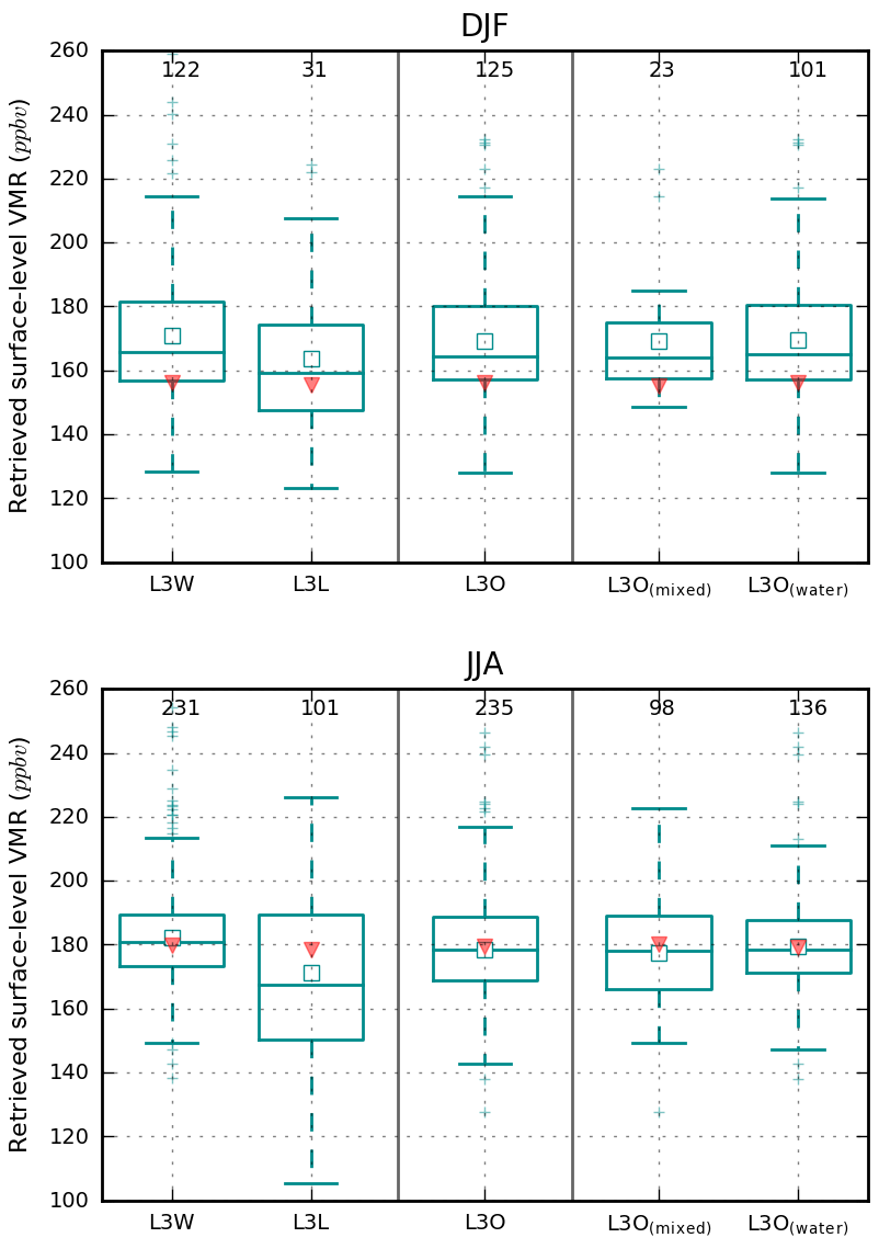
Figure 8Boxplots showing the seasonal distribution of retrieved surface level VMR values from L3W, L3L, L3O, L3O(mixed) and L3O(water). Squares represent mean values; red triangles represent corresponding mean a priori values. Sample sizes are given below the top x axis.
For the same reasons discussed above, L3L also represents the outlier distribution in DJF. Unlike in JJA however, the spread of VMR values is similar in L3L and L3W, likely reflecting the fact that there is some surface level sensitivity in retrievals over both land and water in DJF, allowing for a similar degree of departure from the a priori. The main difference in the distributions is that VMRs in L3L are offset towards lower values. However, the mean difference is not significant between L3L and any of the other time series. Also unlike in JJA, L3L does not necessarily represent the optimal time series for analysing surface level CO in DJF, since retrieval sensitivity is actually higher over water in this season. Information loss resulting from the way L3 products are created is therefore less of an issue than in JJA, owing to the dominance of retrievals over water on the L3O time series (mean surface level AK rowsum is 0.52 for L3O(mixed) vs. 0.43 for L3L and 0.53 for L3W; see Fig. 3). It is worth noting, however, that L3W offers ∼25 % more days with data than L3O(water) in DJF, due to the fact that it gains the retrievals over water that go into L3O(mixed). This is potentially valuable additional temporal information for users of MOPITT products.
Although the sample sizes considered here are different, because L2 retrievals over land and water are not necessarily always present on the same days (e.g. due to variable cloud coverage), the differences in seasonal data distribution discussed in this section hold if the analysis is restricted to only days when L3L and L3W are both present (see Sect. S6). We have only presented analysis for the surface level of the profile here as this is where L3L–L3W differences in retrieved VMRs and retrieval sensitivity are greatest. Plots of other levels are given in Sect. S7.
3.2.2 Consequences for temporal trend analysis
To identify and compare temporal trends in the time series considered above, we perform weighted least squares (WLS) regression analyses on respective seasonal mean profile and TCO values, weighted by the standard deviation of the measurements used in the seasonal mean. For seasons that contain just a single measurement, we use the data record standard deviation scaled by a factor of 100 so as to de-weight these seasons in the fit. All trends identified are detailed in Table 3, and WLS best-fit lines, along with boxplots of seasonal data distributions, are presented for the surface level in Fig. 9. Here, the decreasing trend identified in L3L is over four times stronger than the trend in L3W, a highly significant difference (p<0.01). This is a direct consequence of surface level retrievals over water being tied closely to the a priori owing to their negligible sensitivity, which has no yearly change. This effectively masks the full magnitude of the decrease in CO that appears to be occurring, and which is better detected by retrievals over land owing to their greater sensitivity. Consequently, trends in all L3O subsets are also significantly weaker than the trend in L3L. Since it has some contribution from retrievals over land, L3O(mixed) provides the closest approximation of the trend in L3L, but it is still over 50 % weaker – representing a decrease of 10 % (19 ppbv) over the 15-year period covered by the analysis vs. 21 % (40 ppbv) in L3L. Compared to JJA, trends in surface level VMRs in DJF are far more similar across all the time series, with no significant differences between any of the trends identified. This is attributable to the much smaller differences in retrieval sensitivity over land and water in this season. Thus, while the greater number of days corresponding to the L3W time series makes it of potentially greater value than L3O(water), at least for temporal trend analysis it has no statistical benefit (in fact, users of the original L3 product would seem to get comparable results by performing the analysis on the unfiltered version of L3O).
Table 3Results from WLS regression analysis of seasonal mean L3W, L3L, L3O, L3O(water) and L3O(mixed) time series for selected profile levels in DJF and JJA. Trend corresponds to the gradient of the WLS best-fit line; SE is the standard error of the trend; P value is the probability that the trend is zero; % change per year is the mean percentage change in retrieved CO per year, calculated from WLS regression model predicted values as follows: where ny is the number of years. The penultimate two columns correspond to the result of a significance test performed on the difference between that row's trend and the trend in L3L and L3W, respectively, as follows: where SE1 and SE2 correspond to the standard errors of Trend1 and Trend2 respectively, and Z is the test statistic. Where Z is greater (less) than 1.645 (−1.645), the trend difference is statistically significant to at least 90 % (i.e. p<0.1). Drift is the measurement drift values given in Deeter et al. (2017). No values are given for the 900 and 300 hPa levels of the profile: we therefore cite values for the 400 and 200 hPa levels to give context to the 300 hPa trends we show; and we expect that the 900 hPa level drift is somewhere between that of the surface and 800 hPa levels, which are both shown.

* Units for TCO are molecules per square centimetre (molecules cm−2). n/a: not applicable.
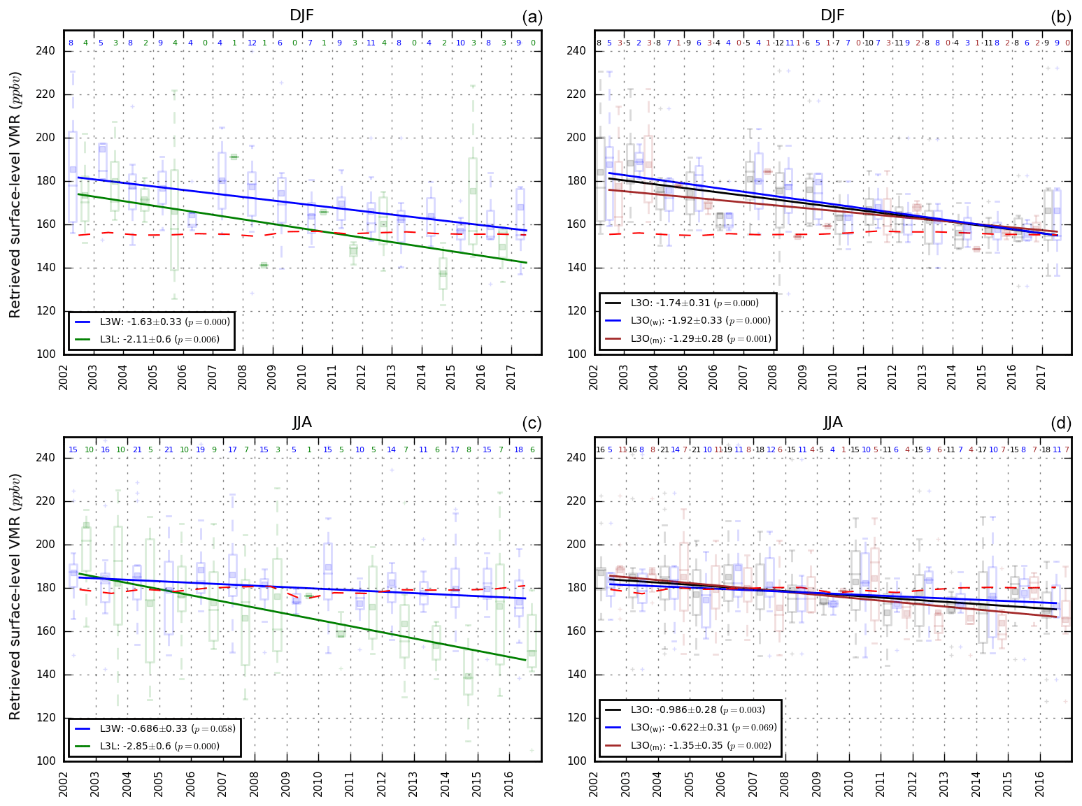
Figure 9WLS regression best-fit lines calculated from seasonal mean retrieved surface VMR time series in DJF (a, b) and JJA (c, d). (a, c) L3L (green) and L3W (blue); (b, d) L3O (black), L3O(mixed) (brown) and L3O(water) (blue). The daily observations corresponding to each seasonal mean value are represented by colour-coded boxplots each year, and the seasonal mean value is represented by filled squares. The dashed red line is the mean of the corresponding seasonal mean a priori data from each of the time series in the respective panel. Colour-coded values below the top x axis correspond to the number of observations each season. Values in the legend are the value, standard error and probability of zero value of the trend, respectively.
Although the land–water retrieval sensitivity contrast remains large at the 900 hPa level in JJA, the trend in L3O(mixed) is a closer match to L3L than at the surface, and the difference loses statistical significance. The loss of information content available in retrievals at the 900 hPa level over land during the creation of L3O (mean 900 hPa AK rowsum is 0.91 for L3L vs. 0.64 for L3O(mixed)) therefore does not have a statistically significant impact on temporal trends identified using L3O(mixed), when compared to L3L. Although the L3L–L3W trend difference is smaller than at the surface level, L3L is still twice as strong as L3W and the difference remains statistically significant. This could be a result of either the retrieval over water still lacking sufficient information to deviate as far from the a priori as the retrieval over land, despite the increase in information content relative to the surface level (mean AK rowsums is 0.15 and 0.44 for the surface and 900 hPa levels respectively); and/or the retrieval at the 900 hPa level over water having a sensitivity peak higher up in the troposphere where CO concentrations may be decreasing at a slower rate than they are closer to the surface, where sensitivity peaks for the 900 hPa level over land (see Fig. 3). By 800 hPa, trends in all time series in JJA have converged, consistent with the further weakening of the land–water sensitivity contrast.
Moving away from the LT, the trends outlined in Table 3 indicate that all time series generally agree on the broad picture: in both seasons, CO concentrations are decreasing in the LT and MT and increasing in the UT, while TCO shows a decrease in DJF and no significant trend in JJA. Although not as pronounced or significant as at the surface in JJA, in all cases there are differences in the magnitude of the identified trend. This is not unexpected given that the seasonal means being regressed differ between time series. As outlined in Sect. 3.1.1 and 3.1.2, temporally coincident retrieved VMRs over land and water do differ in levels of the profile above the LT despite similar retrieval sensitivity at these levels; the differences are just not as systematic as in the LT. However, in addition to the surface and 900 hPa levels in JJA, there are two other instances where trends in L3L and L3W are significantly different: 600 hPa in JJA and 300 hPa in DJF (in both cases there is no statistically significant trend identified in L3L, whereas the trend in L3W is significant). The cause of these discrepancies is not readily apparent given that retrieval sensitivity over land and water is highly comparable in both cases, so further investigation would be needed before we can say with confidence whether or not they have consequences for analyses using the L3O time series, as we have been able to do for the LT.
The main differences in trend discussed above remain if the WLS regression analysis is restricted to only days when L3L and L3W are both present. Results from this restricted analysis are shown in Sect. S8. It is important to note that MOPITT profile measurements are known to have a drift (Deeter et al., 2017), and this should be corrected for in the data if the focus of the analysis is to use them to quantify temporal changes in CO over time. Since the intention of the WLS trend analysis presented here is more illustrative, namely to demonstrate trend differences in the data, we have not corrected for this drift. The results should therefore not be taken out of this context (as well as bias correction, verification against a range of other datasets would be required, especially given the large proportion of missing data). We do however provide the reported drift values in Table 3 for context, which shows that the majority of the trends that we have identified appear to be stronger than the measurement drift (at least for the dataset that has greatest retrieval sensitivity at the respective level of the profile). As noted in Sect. 2.1.1, the measurement drift has been significantly reduced in the latest version of the MOPITT products to be released (MOPITT Version 8; Deeter et al., 2019).
3.3 Consideration of MAM and SON
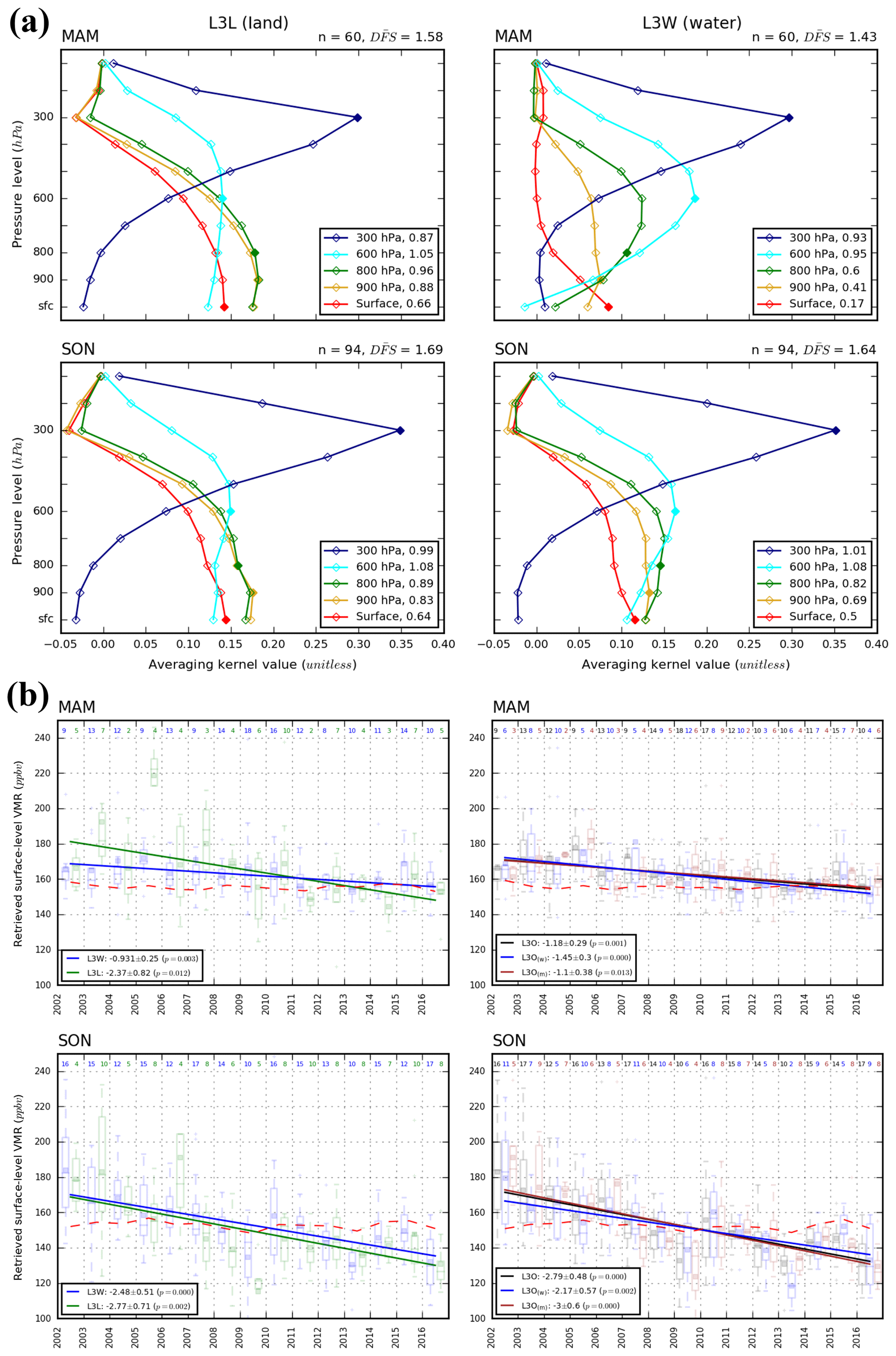
In this paper we have focused only on DJF and JJA for brevity and clarity. The main findings discussed also hold for MAM and SON, however. In MAM, there is a strong sensitivity contrast in the LT between L3L and L3W, similar to that seen in JJA with retrieval sensitivity much greater over land than water (Fig. 10a). As in JJA, the decreasing trend detected in WLS regression analysis of L3L surface level VMRs in MAM is strongly underestimated in L3W and, consequently, in all L3O subsets (Fig. 10b). In SON on the other hand, AKs indicate a much more comparable degree of LT retrieval sensitivity over both land and water; correspondingly, the detected temporal trends are similar in L3L, L3W and L3O subsets.
Users of MOPITT products are advised to filter the data before analysis of profile values in order to maximize the influence of satellite measurements and minimize the impact of a priori CO concentrations on results (MOPITT Algorithm Development Team, 2017; Deeter et al., 2015). In particular, it is advised that retrievals over water, which are known to have lower information content than retrievals over land, are discarded. This is especially so for the analysis of temporal trends in CO concentrations, owing to the year-to-year stationarity of the a priori. However, for L3 grid boxes that straddle the coastline, the ability to apply such filtering is limited since the products will generally have some contribution from L2 retrievals that take place over both land and water. This is a direct consequence of the way that L3 products are created.
As we have explicitly demonstrated for the L3 grid box containing the coastal city of Halifax, Canada, the L2 retrieved CO concentrations, from which the L3 products are created, differ depending on whether the retrieval took place over land or water. In JJA, and especially near the surface, this is directly linked to differences in the sensitivity of the retrievals to the true CO profile. The merging of these retrievals to create the L3 product can significantly affect the statistics of the dataset and the results of temporal trend analysis with the data, with the largest and most statistically significant effects at the surface, where land–water sensitivity contrasts are greatest. As we show, results that are more representative of changes of true CO concentrations close to the surface within the L3 grid box containing Halifax can only currently be obtained by use of the L2 products, which can be filtered by surface type to maximize information content.
Our results suggest that L2 retrievals over land and water should not both contribute to L3 products in coastal grid boxes. This is consistent with previous data filtering recommendations (MOPITT Algorithm Development Team, 2017; Deeter et al., 2015). The horizontally averaged L3L and L3W time series that we have analysed in this paper are effectively L3 land-only and L3 water-only datasets, and these offer an alternative in this respect that preserves the benefits of available L3 products – namely, less computing resources and expertise required for their analysis compared to L2 products, which broadens access to the data – but offers users the flexibility to select over which surface the contributing retrievals were performed in order to maximize the information content of L3 data in coastal grid boxes. Although our study has only focused on the city of Halifax, the results suggest that similar studies be performed for other coastal L3 grid boxes before using MOPITT surface CO, since these contain 6 of the top 10 and 43 of the top 100 agglomerations by population and are therefore likely targets for analysis of temporal changes in air pollution indicators such as CO, especially near the surface. The degree of information content loss in the L3 data will depend on the relative contributions of L2 retrievals over land and water to each specific L3 grid box, as well as on the strength of the land–water retrieval sensitivity difference, which in turn depends on scene-specific geophysical variables such as surface temperature and emissivity. Work is currently ongoing to compare the results of analyses conducted with MOPITT L2 and L3 CO data over these cities.
| ΔRET | Percentage differences in retrieved CO concentrations in L3L and L3W |
| ΔSIM | Percentage differences in simulated retrieved CO concentrations in L3L and L3W |
| AK | Averaging kernel |
| CAM-chem | Community Atmosphere Model with Chemistry |
| CAMS | Copernicus Atmospheric Monitoring Service |
| CAMSRA | CAMS reanalysis |
| CO | Carbon monoxide |
| DFS | Degrees of freedom for signal |
| DJF | December, January, February |
| JJA | June, July, August |
| L2 | Level 2 data products |
| L3 | Level 3 data products |
| L3L | Area-averaged L2 data for the L3 grid box containing Halifax, for L2 retrievals over land only |
| L3O | Original, as-downloaded L3 time series for the L3 grid box containing Halifax |
| L3W | Area-averaged L2 data for the L3 grid box containing Halifax, for L2 retrievals over water only |
| LT | Lower troposphere (surface–800 hPa levels of the profile in MOPITT data) |
| MERRA-2 | NASA Modern-Era Retrospective Analysis for Research and Applications V2 |
| MOPITT | Measurement of Pollution in the Troposphere (instrument) |
| MT | Mid-troposphere (700–500 hPa levels of the profile in MOPITT data) |
| NIR | Near infrared |
| SNR | Signal-to-noise ratio |
| TCO | Total column CO |
| TIR | Thermal infrared |
| Tsfc | Surface air temperature |
| Tskin | Surface skin temperature |
| UT | Lower troposphere (400–100 hPa profile levels in MOPITT data) |
| V7 | MOPITT Version 7 data products |
| VMR | Volume mixing ratio |
| Xapr | A priori CO VMR profile |
| Xapr, sim | A priori CO VMR profile used in retrieval simulation |
| Xrtv | Retrieved CO VMR profile |
| Xsim | Simulated retrieved CO VMR profile |
| Xsim, L3L | Simulated retrieved CO VMR profile from L3L |
| Xsim, L3W | Simulated retrieved CO VMR profile from L3W |
| Xtrue | True CO VMR profile |
| Xtr, sim | True CO VMR profile used in retrieval simulation |
The MOPITT V7 joint TIR-NIR L3 and L2 datasets can be accessed at the following URLs, respectively: https://doi.org/10.5067/TERRA/MOPITT/MOP03J_L3.007 (NASA, 2020a) and https://doi.org/10.5067/TERRA/MOPITT/MOP02J_L2.007 (NASA, 2020b). CAMSRA and ERA-Interim data were downloaded from the ECMWF public datasets portal (https://apps.ecmwf.int/datasets/, last access: 11 June 2020, ECMWF, 2020).
The supplement related to this article is available online at: https://doi.org/10.5194/amt-13-3521-2020-supplement.
IA and AW jointly conceived of and designed the study. IA performed data analysis; both authors examined and interpreted the results and prepared the manuscript.
The authors declare that they have no conflict of interest.
The authors received funding from the Canadian Space Agency through the Earth System Science Data Analyses program (grant no. 16SUASMPTN), the Canadian National Science and Engineering Research Council through the Discovery Grants Program, and Saint Mary's University. We thank the MOPITT team and ECMWF for providing the data used in this study, and we would also like to thank Dylan Jones (University of Toronto) and James Drummond (Dalhousie University) for their helpful discussions, as well as two anonymous reviewers whose helpful comments greatly improved an earlier version of this paper.
This research has been supported by the Canadian Space Agency (grant no. 16SUASMPTN).
This paper was edited by Frank Hase and reviewed by two anonymous referees.
Dee, D. P., Uppala, S. M., Simmons, A. J., Berrisford, P., Poli, P., Kobayashi, S., Andrae, U., Balmaseda, M. A., Balsamo, G., Bauer, P., Bechtold, P., Beljaars, A. C. M., van de Berg, L., Bidlot, J., Bormann, N., Delsol, C., Dragani, R., Fuentes, M., Geer, A. J., Haimberger, L., Healy, S. B., Hersbach, H., Hólm, E. V., Isaksen, L., Kållberg, P., Köhler, M., Matricardi, M., McNally, a. P., Monge-Sanz, B. M., Morcrette, J.-J., Park, B.-K., Peubey, C., de Rosnay, P., Tavolato, C., Thépaut, J.-N., and Vitart, F.: The ERA-Interim reanalysis: configuration and performance of the data assimilation system, Q. J. Roy. Meteor. Soc., 137, 553–597, https://doi.org/10.1002/qj.828, 2011.
Deeter, M. N., Emmons, L. K., Francis, G. L., Edwards, D. P., Gille, J. C., Warner, J. X., Khattatov, B., Ziskin, D., Lamarque, J.-F., Ho, S.-P., Yudin, V., Attié, J.-L., Packman, D., Chen, J., Mao, D., and Drummond, J. R.: Operational carbon monoxide retrieval algorithm and selected results for the MOPITT instrument, J. Geophys. Res., 108, 4399, https://doi.org/10.1029/2002JD003186, 2003.
Deeter, M. N., Edwards, D. P., Gille, J. C., and Drummond, J. R.: Sensitivity of MOPITT observations to carbon monoxide in the lower troposphere, J. Geophys. Res., 112, D24306, https://doi.org/10.1029/2007JD008929, 2007.
Deeter, M. N., Edwards, D. P., Gille, J. C., Emmons, L. K., Francis, G., Ho, S.-P., Mao, D., Masters, D., Worden, H., Drummond, J. R., and Novelli, P. C.: The MOPITT version 4 CO product: Algorithm enhancements, validation, and long-term stability, J. Geophys. Res., 115, D07306, https://doi.org/10.1029/2009JD013005, 2010.
Deeter, M. N., Martínez-Alonso, S., Edwards, D. P., Emmons, L. K., Gille, J. C., Worden, H. M., Pittman, J. V., Daube, B. C., and Wofsy, S. C.: Validation of MOPITT Version 5 thermal-infrared, near-infrared, and multispectral carbon monoxide profile retrievals for 2000–2011, J. Geophys. Res.-Atmos., 118, 6710–6725, https://doi.org/10.1002/jgrd.50272, 2013.
Deeter, M. N., Martínez-Alonso, S., Edwards, D. P., Emmons, L. K., Gille, J. C., Worden, H. M., Sweeney, C., Pittman, J. V., Daube, B. C., and Wofsy, S. C.: The MOPITT Version 6 product: algorithm enhancements and validation, Atmos. Meas. Tech., 7, 3623–3632, https://doi.org/10.5194/amt-7-3623-2014, 2014.
Deeter, M. N., Edwards, D. P., Gille, J. C., and Worden, H. M.: Information content of MOPITT CO profile retrievals: Temporal and geographical variability, J. Geophys. Res.-Atmos., 120, 12723–12738, https://doi.org/10.1002/2015JD024024, 2015.
Deeter, M. N., Edwards, D. P., Francis, G. L., Gille, J. C., Martínez-Alonso, S., Worden, H. M., and Sweeney, C.: A climate-scale satellite record for carbon monoxide: the MOPITT Version 7 product, Atmos. Meas. Tech., 10, 2533–2555, https://doi.org/10.5194/amt-10-2533-2017, 2017.
Deeter, M. N., Edwards, D. P., Francis, G. L., Gille, J. C., Mao, D., Martínez-Alonso, S., Worden, H. M., Ziskin, D., and Andreae, M. O.: Radiance-based retrieval bias mitigation for the MOPITT instrument: the version 8 product, Atmos. Meas. Tech., 12, 4561–4580, https://doi.org/10.5194/amt-12-4561-2019, 2019.
Drummond, J. R., Zou, J., Nichitiu, F., Kar, J., Deschambaut, R., and Hackett, J.: A review of 9-year performance and operation of the MOPITT instrument, Adv. Space Res., 45, 760–774, https://doi.org/10.1016/j.asr.2009.11.019, 2010.
Drummond, J. R., Hackett, J., and Caldwell, D.: Measurements of pollution in the troposphere (MOPITT), in: Optical Payloads for Space Missions, edited by: Shen-En Qian, Wiley and Sons, West Sussex, UK, 639–652, 2016.
Duncan, B. N., Logan, J. A., Bey, I., Megretskaia, I. A., Yantosca, R. M., Novelli, P. C., Jones, N. B., and Rinsland, C. P.: Global budget of CO, 1988–1997: Source estimates and validation with a global model, J. Geophys. Res., 112, D22301, https://doi.org/10.1029/2007JD008459, 2007.
ECMWF: Public Datasets, available at: https://apps.ecmwf.int/datasets/, last access: 11 June 2020.
Edwards, D. P., Halvorson, C. M., and Gille, J. C.: Radiative transfer modeling for the EOS Terra satellite Measurement of Pollution in the Troposphere (MOPITT) instrument, J. Geophys. Res., 104, 16755–16775, https://doi.org/10.1029/1999JD900167, 1999.
Francis, G. L., Deeter, M. N., Martínez-Alonso, S., Gille, J. C., Edwards, D. P., Mao, D., Worden, H. M., and Ziskin, D.: Measurement of Pollution in the Troposphere Algorithm Theoretical Basis Document: Retrieval of Carbon Monoxide Profiles and Column Amounts from MOPITT Observed Radiances (Level 1 to Level 2), Atmospheric Chemistry Observations and Modelling Laboratory, National Center for Atmospheric Research, Boulder, Colorado, available at: https://www2.acom.ucar.edu/sites/default/files/mopitt/ATBD_5_June_2017.pdf (last access: 11 June 2020), 2017.
He, H., Stehr, J. W., Hains, J. C., Krask, D. J., Doddridge, B. G., Vinnikov, K. Y., Canty, T. P., Hosley, K. M., Salawitch, R. J., Worden, H. M., and Dickerson, R. R.: Trends in emissions and concentrations of air pollutants in the lower troposphere in the Baltimore/Washington airshed from 1997 to 2011, Atmos. Chem. Phys., 13, 7859–7874, https://doi.org/10.5194/acp-13-7859-2013, 2013.
Inness, A., Ades, M., Agustí-Panareda, A., Barré, J., Benedictow, A., Blechschmidt, A.-M., Dominguez, J. J., Engelen, R., Eskes, H., Flemming, J., Huijnen, V., Jones, L., Kipling, Z., Massart, S., Parrington, M., Peuch, V.-H., Razinger, M., Remy, S., Schulz, M., and Suttie, M.: The CAMS reanalysis of atmospheric composition, Atmos. Chem. Phys., 19, 3515–3556, https://doi.org/10.5194/acp-19-3515-2019, 2019.
Lamarque, J.-F., Emmons, L. K., Hess, P. G., Kinnison, D. E., Tilmes, S., Vitt, F., Heald, C. L., Holland, E. A., Lauritzen, P. H., Neu, J., Orlando, J. J., Rasch, P. J., and Tyndall, G. K.: CAM-chem: description and evaluation of interactive atmospheric chemistry in the Community Earth System Model, Geosci. Model Dev., 5, 369–411, https://doi.org/10.5194/gmd-5-369-2012, 2012.
MOPITT Algorithm Development Team: MOPITT (Measurements of Pollution in the Troposphere) Version 7 Product User's Guide, Atmospheric Chemistry Observations and Modeling Laboratory, National Center for Atmospheric Research, Boulder, available at: https://www2.acom.ucar.edu/sites/default/files/mopitt/v7_users_guide_201707.pdf (last access: 11 June 2020), 2017.
NASA: MOPITT CO gridded daily means (Near and Thermal Infrared Radiances) V007, Entry ID: MOP03J_7, ESDS, https://doi.org/10.5067/TERRA/MOPITT/MOP03J_L3.007, 2020a.
NASA: MOPITT Derived CO (Near and Thermal Infrared Radiances) V007, Entry ID: MOP02J_7, ESDS, https://doi.org/10.5067/TERRA/MOPITT/MOP02J_L2.007, 2020b.
Pan, L., Edwards, D. P., Gille, J. C., Smith, M. W., and Drummond, J. R.: Satellite remote sensing of tropospheric CO and CH4: forward model studies of the MOPITT instrument, Appl. Optics, 34, 6976–6988, https://doi.org/10.1364/ao.34.006976, 1995.
Pan, L., Gille, J. C., Edwards, D. P., Bailey, P. L., and Rodgers, C. D.: Retrieval of tropospheric carbon monoxide for the MOPITT experiment, J. Geophys. Res., 103, 32277–32290, https://doi.org/10.1029/98JD01828, 1998.
Rodgers, C. D.: Inverse Methods for Atmospheric Sounding, Theory and Practice, World Scientific, Singapore, 2000.
Strode, S. A., Worden, H. M., Damon, M., Douglass, A. R., Duncan, B. N., Emmons, L. K., Lamarque, J.-F., Manyin, M., Oman, L. D., Rodriguez, J. M., Strahan, S. E., and Tilmes, S.: Interpreting space-based trends in carbon monoxide with multiple models, Atmos. Chem. Phys., 16, 7285–7294, https://doi.org/10.5194/acp-16-7285-2016, 2016.
Wiacek, A., Li, L., Tobin, K., and Mitchell, M.: Characterization of trace gas emissions at an intermediate port, Atmos. Chem. Phys., 18, 13787–13812, https://doi.org/10.5194/acp-18-13787-2018, 2018.
Worden, H. M., Deeter, M. N., Edwards, D. P., Gille, J. C., Drummond, J. R., and Nédélec, P.: Observations of near-surface carbon monoxide from space using MOPITT multispectral retrievals, J. Geophys. Res., 115, D18314, https://doi.org/10.1029/2010JD014242, 2010.
Worden, H. M., Deeter, M. N., Frankenberg, C., George, M., Nichitiu, F., Worden, J., Aben, I., Bowman, K. W., Clerbaux, C., Coheur, P. F., de Laat, A. T. J., Detweiler, R., Drummond, J. R., Edwards, D. P., Gille, J. C., Hurtmans, D., Luo, M., Martínez-Alonso, S., Massie, S., Pfister, G., and Warner, J. X.: Decadal record of satellite carbon monoxide observations, Atmos. Chem. Phys., 13, 837–850, https://doi.org/10.5194/acp-13-837-2013, 2013.
Worden, H. M., Deeter, M. N., Edwards, D. P., Gille, J., Drummond, J., Emmons, L. K., Francis, G., and Martínez-Alonso, S.: 13 years of MOPITT operations: Lessons from MOPITT retrieval algorithm development, Ann. Geophys.-Italy, 56, 1–5, https://doi.org/10.4401/ag-6330, 2014.
Available at https://eosweb.larc.nasa.gov/sites/default/files/project/mopitt/quality_summaries/mopitt_level3_ver6.pdf (last access: 11 June 2020).