the Creative Commons Attribution 4.0 License.
the Creative Commons Attribution 4.0 License.
 | 10 Jul 2020
Preliminary investigation of the relationship between differential phase shift and path-integrated attenuation at the X band frequency in an Alpine environment
Guy Delrieu
Anil Kumar Khanal
Nan Yu
Frédéric Cazenave
Brice Boudevillain
Nicolas Gaussiat
The RadAlp experiment aims at developing advanced methods for rainfall and snowfall estimation using weather radar remote sensing techniques in high mountain regions for improved water resource assessment and hydrological risk mitigation. A unique observation system has been deployed since 2016 in the Grenoble region of France. It is composed of an X-band radar operated by Météo-France on top of the Moucherotte mountain (1901 m above sea level; hereinafter MOUC radar). In the Grenoble valley (220 m above sea level; hereinafter a.s.l.), we operate a research X-band radar called XPORT and in situ sensors (weather station, rain gauge and disdrometer). In this paper we present a methodology for studying the relationship between the differential phase shift due to propagation in precipitation (Φdp) and path-integrated attenuation (PIA) at X band. This relationship is critical for quantitative precipitation estimation (QPE) based on polarimetry due to severe attenuation effects in rain at the considered frequency. Furthermore, this relationship is still poorly documented in the melting layer (ML) due to the complexity of the hydrometeors' distributions in terms of size, shape and density. The available observation system offers promising features to improve this understanding and to subsequently better process the radar observations in the ML. We use the mountain reference technique (MRT) for direct PIA estimations associated with the decrease in returns from mountain targets during precipitation events. The polarimetric PIA estimations are based on the regularization of the profiles of the total differential phase shift (Ψdp) from which the profiles of the specific differential phase shift on propagation (Kdp) are derived. This is followed by the application of relationships between the specific attenuation (k) and the specific differential phase shift. Such k–Kdp relationships are estimated for rain by using drop size distribution (DSD) measurements available at ground level. Two sets of precipitation events are considered in this preliminary study, namely (i) nine convective cases with high rain rates which allow us to study the ϕdp–PIA relationship in rain, and (ii) a stratiform case with moderate rain rates, for which the melting layer (ML) rose up from about 1000 up to 2500 m a.s.l., where we were able to perform a horizontal scanning of the ML with the MOUC radar and a detailed analysis of the ϕdp–PIA relationship in the various layers of the ML. A common methodology was developed for the two configurations with some specific parameterizations. The various sources of error affecting the two PIA estimators are discussed, namely the stability of the dry weather mountain reference targets, radome attenuation, noise of the total differential phase shift profiles, contamination due to the differential phase shift on backscatter and relevance of the k–Kdp relationship derived from DSD measurements, etc. In the end, the rain case study indicates that the relationship between MRT-derived PIAs and polarimetry-derived PIAs presents an overall coherence but quite a considerable dispersion (explained variance of 0.77). Interestingly, the nonlinear k–Kdp relationship derived from independent DSD measurements yields almost unbiased PIA estimates. For the stratiform case, clear signatures of the MRT-derived PIAs, the corresponding ϕdp value and their ratio are evidenced within the ML. In particular, the averaged PIA∕ϕdp ratio, a proxy for the slope of a linear k–Kdp relationship in the ML, peaks at the level of the copolar correlation coefficient (ρhv) peak, just below the reflectivity peak, with a value of about 0.42 dB per degree. Its value in rain below the ML is 0.33 dB per degree, which is in rather good agreement with the slope of the linear k–Kdp relationship derived from DSD measurements at ground level. The PIA∕ϕdp ratio remains quite high in the upper part of the ML, between 0.32 and 0.38 dB per degree, before tending towards 0 above the ML.
- Article
(3007 KB) - Full-text XML
- BibTeX
- EndNote


Estimation of atmospheric precipitation (solid/liquid) is important in a high mountain region such as the Alps for the assessment and management of water and snow resources for drinking water, hydropower production, agriculture and tourism characterized by high seasonal variability. One of the most critical applications concerns the prediction of natural hazards associated with intense precipitation and melting of snowpacks, i.e., inundations, floods, flash floods and gravitational movements, which requires a high-resolution observation, namely spatial resolution ≤1 km2 and temporal resolution ≤1 h. While this can hardly be achieved over extended areas with traditional in situ rain gauge networks, the use of radar remote sensing has a high potential that needs to be exploited but also a number of limitations that need to be surpassed. Quantitative precipitation estimation (QPE) with radar remote sensing in a complex terrain such as the Alps is made challenging by the topography and the space–time structure and the dynamics of precipitation systems. Radar coverage of the mountain regions brings the following dilemma. On the one hand, installing radar at the top of a mountain allows for a 360∘ panoramic view and therefore the ability to detect precipitation systems over a long range at the regional scale. This is particularly relevant for localized and heavy convective systems in warm seasons. But the precipitation is likely to undergo a significant change between detection and arrival at ground level, including a phase change when the 0 ∘C isotherm is located at the level of or lower than the radar beam altitude. Such situations are likely to be frequent during cold periods, with a strong impact on QPE quality at ground level. On the other hand, installing a radar at the bottom of the valley provides high-resolution and quality data required for vulnerable and densely populated Alpine valleys, but the QPEs are limited in the latter due to beam blockage by surrounding mountains.
In Europe, MeteoSwiss has the longest-standing experience in operating radars in mountainous regions. The Swiss C-band radar network in the Alps (Joss and Lee, 1995; Germann et al., 2006) is one of the highest in the world and is coping with the associated altitude dilemma by using a large number of plan-position indicator (PPI) scans (including negative elevation ones) aimed at determining high-resolution vertical profiles of reflectivity. Sophisticated radar–rain gauge merging techniques and echo-tracking techniques, as well as numerical prediction models outputs (Sideris et al., 2014; Foresti et al., 2018) are implemented to better understand and quantify the complexity of precipitation distribution in such a rugged environment. More recently, Météo-France has chosen to complement the coverage of its operational radar network of Application Radar à la Météorologie Infra-Synoptique (ARAMIS) in the Alps by means of X-band polarimetric radars. A first set of three radars was installed in the southern Alps within the Risques Hydrométéorologiques en Territoires de Montagnes et Méditerranéens (RHyTMME) project in the period 2008–2013 at Montagne de Maurel (1770 m above sea level; hereinafter a.s.l.), Mont Colombis (1740 m a.s.l.) and Vars Mayt (2400 m a.s.l.; Westrelin et al., 2012). This effort was continued in 2014–2015 with the installation of an additional X-band radar system (hereinafter MOUC radar) on top of the Moucherotte mountain (1920 m) that dominates the valley of Grenoble, the biggest city in the French Alps with about 500 000 inhabitants. The choice of the X-band frequency is challenging due to its sensitivity to attenuation (e.g., Delrieu et al., 2000). In the past, the Institute of Environmental Geosciences (IGE) radar team has proposed the so-called mountain reference technique (MRT; Delrieu et al., 1997; Serrar et al., 2000; Bouilloud et al., 2009) to take advantage of this drawback for both correcting the gate-to-gate attenuation and performing a self-calibration of the radar. The idea was to estimate the path-integrated attenuations (PIAs) in some specific directions from the decrease in mountain returns during rainy periods. Such PIA estimates were then used as constraints for backward or forward attenuation correction algorithms (Marzoug and Amayenc, 1994) with optimization of an effective radar calibration error, given a drop size distribution (DSD) parameterization. The development of polarimetric radar techniques (e.g., Bringi and Chandrasekar, 2001; Ryzhkov et al., 2005) has allowed a scientific breakthrough for quantitative precipitation estimation (QPE) at X band by exploiting the relationship which exists between the specific differential phase shift on propagation (Kdp, in ) and the specific attenuation k (dB km−1). As with the MRT, the differential propagation phase Φdp(r2)−Φdp(r1) over a given path (r1,r2) can be used to estimate PIA(r1,r2), which can constrain a backward attenuation correction algorithm and allow a self-calibration of the radar and/or an adjustment of the DSD parameterization (Testud et al., 2000; Ryzhkov et al., 2014). Two major advantages of the polarimetric technique over the MRT can be formulated, namely (1) the availability of PIA constraints for any direction with significant precipitation and (2) the subsequent possibility of using a backward attenuation correction algorithm, which is known to be stable, while the forward formulation is inherently unstable. Accounting for their respective potential in different rain regimes (moderate to heavy), some combined algorithms making use of various polarimetric observables (reflectivity, differential reflectivity and specific differential phase shift on propagation) have also been proposed for the X-band frequency (e.g., Matrosov and Clark, 2002; Matrosov et al., 2005; Koffi et al., 2014). Although the polarimetric QPE methodology is now quite well established and validated for rainy precipitation (Matrosov et al., 2005; Anagnostou et al., 2004; Diss et al., 2009), Yu et al. (2018) have shown, in their first performance assessment of the RHyTMME radar network, the limitations associated with the use of polarimetric X-band radars in mountainous regions. They have pointed out (i) the need to better understand and quantify attenuation effects in the melting layer (ML), (ii) the importance of nonuniform beam filling (NUBF) effects at medium-to-long ranges in such a high-mountain context, and (iii) the stronger impact of radome attenuation at X band compared to S or C band. Yu et al. (2018) also had a first attempt at studying the relationship between the specific differential phase shift on propagation and the specific attenuation in the melting later by using the collocated measurements of two X-band radars, one situated well below and the other one situated well above the 0 ∘C isotherm, and by considering the attenuation uniform within the ML.
Since 2016, we have had the opportunity to operate a research X-band polarimetric radar system (hereinafter XPORT radar) at IGE at the bottom of the Grenoble valley. This unique facility, consisting of two radar systems 11 km apart and operating on an altitudinal gradient of about 1700 m, should enable us to make progress on how to deal with the altitude dilemma and the potential/issues associated with the choice of the X-band operating frequency. Following a first article based on the RadAlp experiment about the characterization of the melting layer (Khanal et al., 2019), we concentrate hereinafter on the relationship between total differential phase shift (ϕdp) derived from polarimetry and PIAs derived from the MRT. In Sect. 2, we present the observation system available and contrast rainy events considered in this study as follows: (i) a set of nine convective events with high rain rates, for which the melting layer was well above the detection domain of the XPORT radar, allows us to study the ϕdp−PIA relationship in rain; and (ii) a stratiform case with moderate rain rates, for which the melting layer rose up from about 1000 to 2500 m a.s.l., allows us to perform a horizontal scanning of the ML with the MOUC radar and a preliminary analysis of the ϕdp−PIA relationship in the various layers of the ML. We present and illustrate, in Sect. 3, the methodology used for the PIA and ϕdp estimation. We also investigate the relationship between the specific differential phase shift on propagation (Kdp) and the specific attenuation (k) thanks to drop size distribution (DSD) measurements collected in the Grenoble valley during the two sets of events. The results concerning the ϕdp–PIA relationship in rain and in the ML are presented and discussed in Sect. 4, while conclusions and perspectives are drawn in Sect. 5.
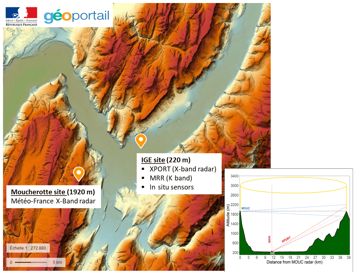
Figure 1The topographical map of Grenoble is shown along with the positions of two radar systems. A vertical cross section along the line joining the two radar sites is shown in the insert at the bottom right of the figure.
2.1 Observation system
Grenoble is a y-shaped alluvial valley in the French Alps, with a mean altitude of about 220 m a.s.l. and surrounded by three mountain ranges, namely the Chartreuse (culminating at 2083 m a.s.l.) to the north, the Belledonne (2977 m) to the southeast and the Vercors (2307 m) to the west. Figure 1 shows the topography of the area and the positions of the Météo-France radar system on top of the Moucherotte mountain and the IGE experimental site at the bottom of the valley.
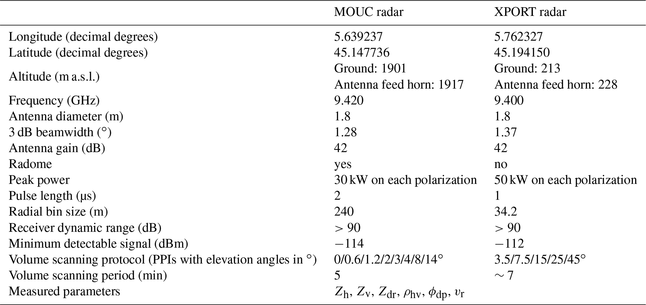
Among other devices, the IGE experimental site includes the following: (i) the IGE XPORT research radar (Koffi et al., 2014; see Table 1 for the list of its main parameters); (ii) one Micro Rain Radar (MRR; not used in the current study); (iii) one meteorological station including pressure, temperature, humidity, wind probes and several rain gauges; and (iv) one Parsivel2 disdrometer. The characteristics of the MOUC radar are listed in Table 1. XPORT radar was built in the laboratory in the 2000s. It was operated during more than 10 years in western Africa within the African Monsoon Multidisciplinary Analysis (AMMA) and Megha-Tropiques calibration/validation campaigns. Since its return to France in 2016, a maintenance and updating program has been underway to improve its functionalities, notably with respect to the real-time data processing and the antenna control program. One noticeable feature of XPORT radar is the range bin size of 34.2 m (which actually corresponds to an oversampling since, for a pulse width of 1 µs, the theoretical bin size is 150 m), which is an interesting figure for the close-range and volumetric measurements considered in this study. Note that while the MOUC radar is operated 24 h per day and its data are integrated in the Météo-France mosaic radar products, the XPORT radar is operated with alerts only on for significant precipitation events.
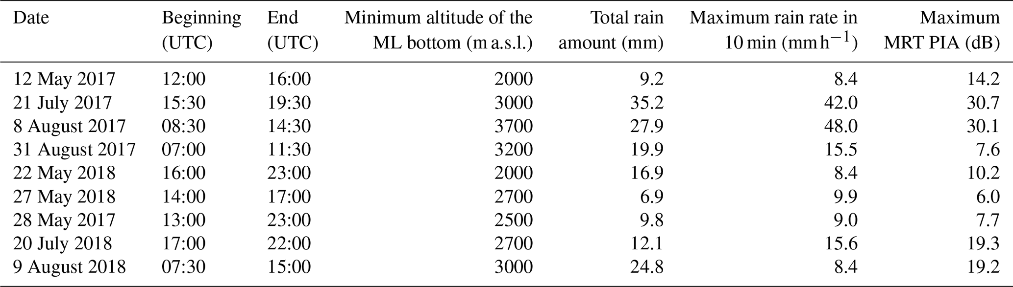
Table 2Some characteristics of the nine convective events considered in the study of the ϕdp–PIA relationship in rain. The ML detection was performed with the 25∘ elevation angle measurements of the XPORT radar using the algorithm described in Khanal et al. (2019). The total rain amount and the maximum rain rate are recorded at the weather station available at the XPORT radar site at IGE. The maximum PIA is derived from the MRT by considering the 7.5∘ elevation data of the XPORT radar.
2.2 Dataset
Table 2 shows the main characteristics of the nine convective events considered for the study of the ϕdp–PIA relationship in rain, by using the XPORT radar data. A stratiform event, which occurred on 3–4 January 2018, is also considered for a preliminary study of the ϕdp–PIA relationship in the ML, with both the MOUC and the XPORT radar data. Figure 2 presents a time series of one of the most intense convective event (21 July 2017) and the stratiform event. In both cases, the total rain amount observed at the IGE site was about 35 mm, but in 3 h, with two peak rain rates of about 40 mm h−1 for the 21 July 2017 convective event, while the 3–4 January 2018 stratiform event lasted more than 12 h with an average rain rate of about 3 mm h−1. The two events also differ in their vertical structure. The bottom graphs of Fig. 2 display the time series of the altitudes of the tops, peaks and bottoms of the horizontal reflectivity (Zh) and copolar correlation coefficient (ρhv) signatures of the ML, obtained with the automatic detection algorithm described in Khanal et al. (2019). The quasi-vertical profiles (QVP; Ryzhkov et al., 2016) derived from the XPORT 25∘ PPIs are considered in the ML detection. For the convective case, the ML extends from 3000 to 4000 m a.s.l. and more, i.e., well above the altitudes of the two radars. Table 2 indicates that this is also the case for the other convective events – at least for the XPORT radar. For the stratiform event, the ML extends between 800 and 1500 m a.s.l. during the first part of the event (between 3 January, 20:00 UTC, and 4 January, 01:30 UTC) and then rises in about 2 h to stabilize at an altitude range of about 2200–2800 m a.s.l. after 04:00 UTC, passing progressively at the level of the MOUC radar in the meantime.
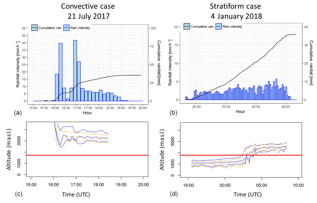
Figure 2Description of two rain events considered in the present study: (a, c) convective case of 21 July 2017 and (b, d) stratiform case of 4 January 2018. (a, b) Rain rate and cumulative rainfall time series observed at the IGE site and (c, d) results of the ML detection algorithm based on XPORT 25∘ PPI data. The horizontal red line indicates the altitude of the MOUC radar (see text for details).

Figure 3Examples of XPORT 7.5∘ PPIs of raw reflectivity (not corrected for attenuation) taken for two time steps during the 21 July 2017 convective event. The crosses indicate the location of the two radars and the black/white (5/10 km) range markers correspond to the XPORT and the MOUC radar, respectively. The red circles highlight the mountain returns associated with the Chamrousse (southeast) and the Moucherotte (southwest) mountains in between the 10–15 km range.
As an additional illustration of the dataset, Fig. 3 gives two examples of XPORT PPIs at 7.5∘ elevation angle for moderate (left) and intense (right) rain during the 21 July 2017 event. As a clear feature, one can see that, for this elevation angle, the radar beam is fully blocked by the Chartreuse mountain range in the northern sector. Also visible in the northeastern sector and, to a lesser extent, in the southwestern sector are partial beam blockages associated with tall trees in the vicinity of the XPORT radar on the Grenoble campus. This figure is also intended to draw the attention of the reader to the decrease in the Chamrousse and Moucherotte mountains returns (within red circles) during the intense rain time step, compared to their values in moderate rain, as a first illustration of the MRT principle.
Our aim is to study the relationship between two radar observables of propagation effects at X band, namely path-integrated attenuation and differential propagation phase due to precipitation occurring along the radar path. We describe, in the following two subsections, the estimation methods that were implemented. In Sect. 3.3, we complement the methodology description with the presentation of DSD-derived k–Kdp relationships.
3.1 Path-integrated attenuation estimation
Let us express the PIAs (in dB) at a given range r (km) as follows:
where k(s) (dB km−1) is the specific attenuation due to rain at range s (km). r0 is the range where the measurements start to become exploitable, i.e., the range where measurements are free of ground clutter associated with side lobe effects. The term PIA(r0) represents the so-called on-site attenuation resulting from radome attenuation and range attenuation at range closer than r0. Note that PIAs can be obtained from Eq. (1) for both the horizontal and the vertical polarizations. In the present article, we will restrict ourselves to the horizontal polarization, as the study of differential attenuation is a possible topic for a future study. Delrieu et al. (1999) have proposed an assessment of the quality of PIA estimates from mountain returns by implementing a receiving antenna in the Belledonne mountain range in conjunction with an X-band radar operated on the Grenoble campus. They found good agreement between the two PIA estimates for PIAs exceeding the natural variability of the mountain reference target during dry weather. They recommended using strong mountain returns (greater than, e.g., 50 dBZ during dry weather) so as to minimize the impact of precipitation falling over the reference target itself. They also point out that this approach is not able to separate the effects of on-site and range attenuation. They verified, however, by implementing the receiving antenna close to the radar (at a range of about 200 m), that the on-site attenuation was negligible for a radomeless radar, which is the case for the XPORT radar but not for the MOUC radar. Another interesting feature of the MRT PIA estimator is its independence with respect to eventual radar calibration errors.
In the current study, we used the following procedure to determine the mountain reference targets for the XPORT radar.
Table 3Geometrical characteristics and apparent reflectivity statistics for the 16 mountain targets selected for the XPORT radar at an elevation angle of 7.5∘. The mean, standard deviation, and 10 % and 90 % quantiles of the apparent reflectivity time series are given for the first and last convective events in the considered period (see Table 2).
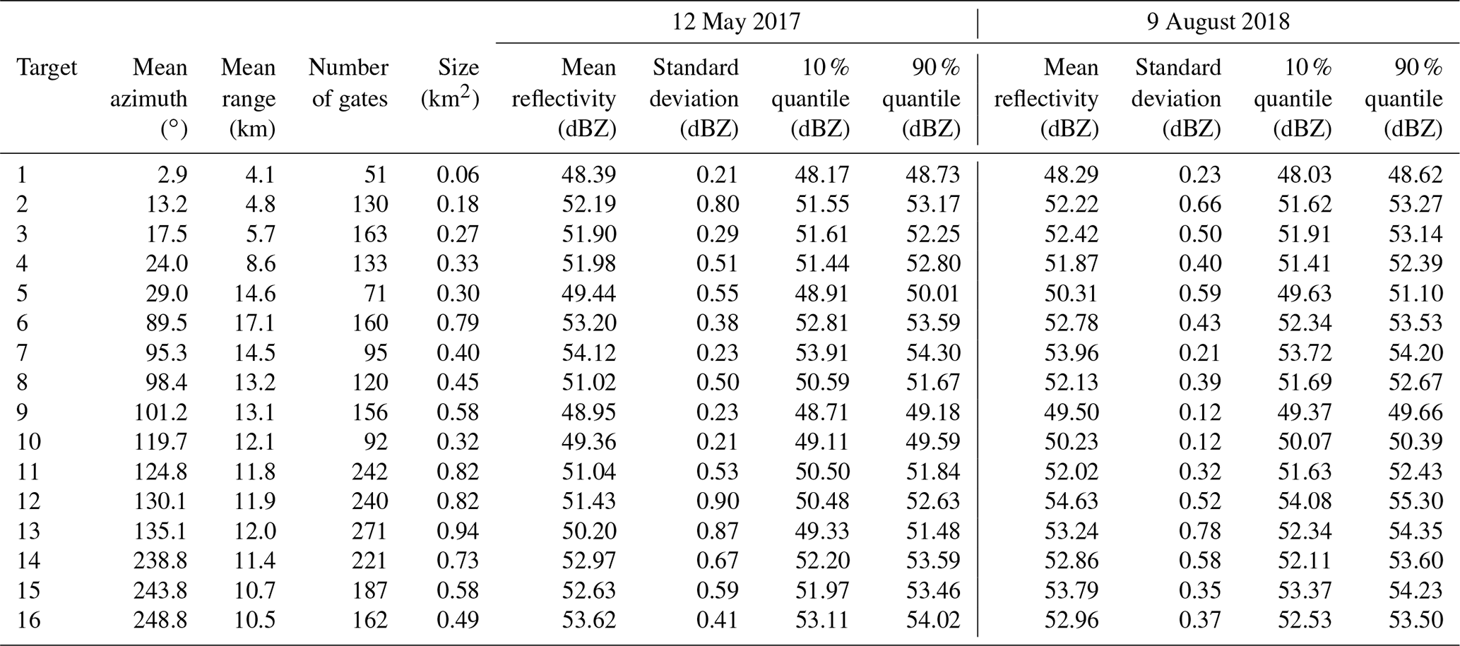
A large series of raw reflectivity data, observed during widespread rainfall with no ML contamination, was accumulated and averaged in order to characterize the detection domain of the XPORT radar at the 7.5∘ elevation angle. This allowed us to determine the mountain returns, the full beam blockages due to mountains, the partial beam blockages due to tall trees and spurious detections due to side lobes in the vicinity of the radar. A manual selection of the mountain reference targets was then performed based on the map of the apparent reflectivity above 45 dBZ. The targets, made up of mountain returns from successive radials (up to 9) with a limited range extent (less than 2.0 km), are described in Table 3. Based on the radar equation and the receiver characteristics, care was taken to discard targets eventually subject to saturation at close range. The selected targets are located at a mean range between 4.1 and 17.1 km and have sizes between 0.06 and 0.94 km2. For each rain event, dry weather data before and/or after the event were used to characterize the mean target reflectivity and its time variability. Note that the mean reflectivity for each target and each time step was computed as the average of the dBZ values of each radial gate comprising the target. This is justified by the fact that we aim at estimating PIAs in dB. Table 3 lists the mean, standard deviation and 10 % and 90 % quantiles of the time series of the dry weather apparent reflectivity of the reference targets for the first and last event of the considered series. One can notice the good stability of the mean reflectivity values between the two events, which is an indication of both the radar calibration stability during the period and the moderate impact of the mountain surface conditions already evidenced in previous studies (Delrieu et al., 1999; Serrar et al., 2000). The standard deviations of the reflectivity time series range between 0.2 and 0.9 dBZ, and the mean 10 %–90 % interquantile range is equal to 1.03 dBZ.
Table 4Geometrical characteristics and apparent reflectivity statistics for the 13 mountain targets selected for the MOUC radar at an elevation angle of 0∘. The mean, standard deviation, and 10 % and 90 % quantiles of the apparent reflectivity time series are computed over the period of 3 January 2018 from 19:00 to 23:55 UTC, preceding the rising of the ML at the level of the MOUC radar.
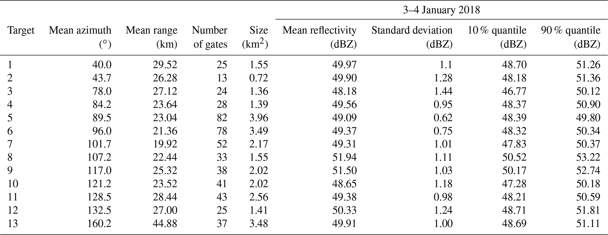
Due to limited data availability, a simpler approach was implemented for the selection of the MOUC mountain reference targets. Here again, the raw reflectivity data were accumulated and averaged, but only over the period of 3 January 2018, 19:00–23:55 UTC, preceding the rise of the ML at the level of the MOUC radar. It was snowing during this period at the MOUC radar site. So, we are implicitly making the assumption of negligible attenuation during snowfall (supported by the literature; e.g., Matrosov et al., 2009) in the considered case study. Table 4 displays the geometrical characteristics of the targets, as well as the mean, standard deviation and 10 % and 90 % quantiles of their apparent reflectivity time series. Targets are located at greater distances than those of the XPORT radar, i.e., between 19.9 and 44.9 km. In spite of having larger sizes (between 0.7 and 4.0 km2), this range effect probably explains why their standard deviations are higher, namely between 0.75 and 1.44 dBZ. The 10 %–90 % interquantile ranges are subsequently higher as well, with a mean value of 2.6 dBZ.
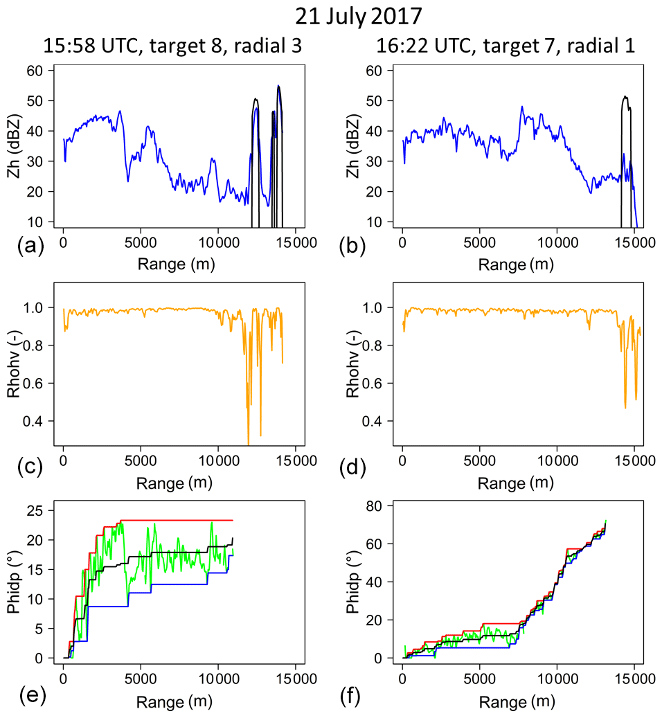
Figure 4Two examples (right and left columns) of Zh, ρhv, and ϕdp range profiles of the XPORT radar (7.5∘ PPI) during the 21 July 2017 convective event for one radial of a given mountain target. The raw horizontal reflectivity profiles (a, b) at the considered time steps (blue) are displayed together with the dry weather reference target value (black). The ρhv profiles (c, d) are used to detect the rainy gates not affected by clutter at close range and in the region of the mountain target. Panels (e) and (f) display the raw ψdp profiles (green), the upper (red) and lower (blue) envelope curves, and the regularized ϕdp profiles (black).
The top graphs of Fig. 4 give two examples of apparent reflectivity profiles for a radial of a given target during the 21 July 2017 rain event. The example on the left-hand side corresponds to a moderate PIA (5.4 dB, when considering all the gates of the radials comprising the target) and the right-hand side example corresponds to one of the highest PIA value observed (27.6 dB) in our dataset. We tried to limit, as far as possible, the radial extent of targets (less than 2000 m) and/or multipeaks targets, such as the one shown in the left-hand side example, in order to limit positive bias on MRT PIA estimates. The top graphs of Fig. 5 give two examples of apparent reflectivity time series during the events of 21 July 2017 and 20 July 2018, together with the mean, 10 % and 90 % quantiles of the dry weather apparent reflectivity. For both cases, the XPORT data acquisition started a bit after the actual beginning of the storm. Therefore, the dry weather reference values were estimated with data collected after the event, i.e., between 19:00 and 22:00 UTC for the 21 July 2017 event and between 00:00 and 06:00 UTC on the day after for the 20 July 2018 event. For these convective events, one can note the erratic nature of the apparent reflectivity time series at the XPORT radar acquisition period used at that time (about 7 min). The MRT PIA estimates are simply calculated as the difference between the mean values of the target apparent reflectivity during dry weather and at each time step of the rain event (blue lines in the bottom graphs of Fig. 5).
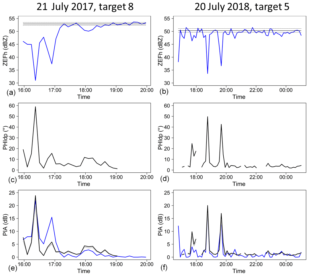
Figure 5Two examples of time series of the apparent reflectivity of mountain returns for a given target (a, b), the corresponding Φdp estimates (c, d), and the resulting PIA estimates. The horizontal black lines in the top graphs represent the mean (solid line) and the 10 % and 90 % quantiles (broken lines) of the dry weather apparent reflectivity of the target. The three lines in (e) and (f) correspond to the MRT PIA estimates (blue) and to the polarimetry-derived PIA estimates by using the linear k–Kdp relationship (gray) and the nonlinear k–Kdp relationship (black) derived from DSD measurements at ground level.
3.2 Differential propagation phase estimation
Let us express the total differential phase shift between copolar (HH and VV) received signals as follows:
where Kdp(s) is the specific differential phase shift on propagation (∘ km−1) related to precipitation at any range s between r0 and r, and δhv(r) is the differential phase shift on backscatter (∘) at range r.
The quantity of interest, i.e., the differential propagation phase associated with precipitation along the path, is denoted as follows:
As with the on-site attenuation for the MRT, we have a problem here with the possible influence of the differential phase shift on backscatter δhv(r) that may introduce a positive bias on the estimation of the differential phase shift associated with precipitation along the path. In the literature (e.g., Otto and Russchenberg, 2011; Schneebeli and Berne, 2012) we find power law relationships between δhv and Zdr at X band in rain, giving values for the differential phase shift on backscatter in the ranges of [0.6–1.0∘] and [2.1–3.5∘] for the differential reflectivity of 1 and 2 dB, respectively. Scattering simulations based on disdrometer data (Trömel et al., 2013) indicate that quite a large scatter may exist with respect to such power law models, and there is an important influence from the considered hydrometeor temperature. From simulations based on radar data at various frequencies, the same authors quantify δhv(r) values as high as 4∘ in the ML at X band and mention that strong δhv(r) values may be associated with both large dry hailstones and wet hailstones, especially at X band. Let us note that no hail was reported for the convective cases considered in the present study. Keeping the related orders of magnitude in mind, and the fact that significant δhv effects are associated with bumps in the ψdp profiles, hereafter we will carefully discuss the possibility of assuming δhv to be negligible, or not, with respect to ϕdp.
In this study, the following method was implemented for the processing of the ψdp profiles and the subsequent estimation of ϕdp values near the mountain targets for the XPORT radar (rain case based on convective events).
We first determined so-called rainy range gates along the path by using the ρhv profiles. The raw ψdp(r) values, for which ρhv(r) was less than 0.95 (empirical threshold with limited impact in the [0.95–0.97] range), were set to missing values. In addition, we defined the beginning of the rainy range by determining the first series of 10 successive gates (again, an empirical choice corresponding to a range extent of 342 m) overpassing this threshold. The r0 value was set to the minimum range value of this series. Similarly, we defined the end of the rainy range by determining the last series of 10 successive range gates overpassing this threshold close to the mountain target. A maximum rainy range, denoted as rM, was defined as the maximum range value of this series. It is noteworthy to mention that rain likely occurs in the ranges less than r0 and greater than rM and in the intermediate ranges for which the ψdp(r) values were set to missing values. It is, however, critical to discard such gates that may be prone to clutter due to side lobes close to the radar or mountain returns close to the mountain target. Although the intermediate missing values will not impact the ϕdp estimation, we have to mention that both the initial and final missing values may result in a negative bias on the PIA estimation based on ϕdp(rM).
In the current version of the procedure, every single radial was processed separately. First, an unfolding was applied by adding 360∘ to negative ψdp(r) values. The system differential phase shift was estimated as the median of the ψdp(r) values corresponding to the beginning of the rainy range. This value was subtracted from the raw ψdp(r) profiles, and eventual negative values were set to 0. Regarding the ψdp measurement noise processing, we have implemented and improved a regularization procedure initially proposed by Yu and Gaussiat (2018). This procedure consists of defining an upper envelope curve, starting from r0, and a lower envelope curve, starting from rM, by considering a maximum jump, denoted as diffmax, authorized between two successive gates. The calculation was performed for a series of diffmax values in the range of 0.5–10∘. The regularized ψdp profiles (increasing monotonous curves) were estimated by taking the average of the upper and lower envelope curves. Note that the values for the missing gates between r0 and rM were simply interpolated with the adjacent values of the regularized profile. A mean absolute difference (MAD) criterion between the raw and regularized profiles over a series of 30 gates with nonmissing values near the mountain target (an empirical choice corresponding to a range extent of about 1 km) was used to determine the optimal diffmax value and the associated profile. The optimal profile was finally selected if the MAD criterion was less than 50 %, otherwise we considered the polarimetry-derived PIAs to be missing for the considered radial. Finally, the ϕdp(rM) value for the target was estimated as a weighted average of the ϕdp(rM) values of all the nonmissing radials composing the target, with the weights being the number of reference gates of each radial. The bottom graphs of Fig. 4 present the raw and regularized profiles, and the envelope curves, for the examples already commented on above. For the right-side hand example corresponding to one of the strongest PIAs (27.6 dB) observed, one can note that the noise of the raw ψdp profile is low, especially in the range with the highest gradients between 7 and 13 km. There is no apparent bump on the raw profile that could signal a δhv contamination so that one might be tempted to consider the regularized profile as a good estimator of the ϕdp profile in that case. The left-hand side example, corresponding to a moderate MRT-derived PIA of 5.4 dB, is more complex. As already noted, the mountain target itself is noisy with significant mountain return contamination before range rM, as evidenced by the ρhv profile. In addition, one can note a nonmonotonic behavior of the raw ψdp profile, with a plateau of about 17.5∘ for ranges greater than 4 km, following an increase in the raw profile (with moderate noise) up to 22∘ at a 4 km range. One might assume that there is a δhv contamination in that case. Interestingly, the regularization procedure is shown to provide a good filtering of the bump, and here again we are tempted to consider the regularized profile as a good estimator of the ϕdp profile. The middle graphs in Fig. 5 display the time series of the ϕdp(rM) values associated with the apparent reflectivity of the mountain returns discussed above. One can note good consistency in the two time series for the highest peaks, while discrepancies can be evidenced for the moderate and small values.
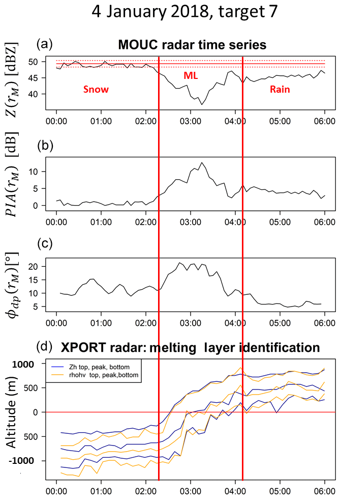
Figure 6Time series of (a) the apparent reflectivity values of a given mountain reference target together with the dry weather reference (solid red horizontal lines for the mean) and the 10 % and 90 % quantiles (broken red lines), (b) the resulting PIA estimates (dB), and (c) the corresponding ϕdp(rM) values (∘) for the 0∘ PPI of the MOUC radar during the 3–4 January 2018 stratiform rain event. (d) displays the results of the ML detection algorithm performed with the XPORT 25∘ PPI data (see text for details).
Basically, the same methodology was implemented for the MOUC radar case study, with some alterations to be described hereafter. Figure 6 provides the time series of the apparent reflectivity of a given mountain target, the resulting PIA estimates and the ϕdp(rM) estimates for the 0∘ PPI of the MOUC radar during the stratiform event of 3–4 January 2018. The time period considered in the figure ranges from 00:00 to 06:00 UTC on 4 January 2018 in order to focus on the rising of the ML between 02:00 and 04:00 UTC. The target is located at a distance of 19.9 km from the radar. The bottom graph of Fig. 6 displays the results of the ML detection algorithm (Khanal et al., 2019) in terms of the altitudes of the top, peak and bottom of the Zh (blue) and the ρhv (orange) ML signatures. The altitude of the Zh top inflexion point is assumed to correspond to the 0 ∘C isotherm altitude, while the ρhv bottom inflexion point corresponds well with the bottom of the ML according to Khanal et al. (2019). We therefore define the ML width as the altitude difference between Zh top and ρhv bottom. Before 02:00 UTC, the ML is well below the altitude of the MOUC radar. MOUC radar measurements at the 0∘ elevation angle are therefore made in snow/ice precipitation during this period. Based on the ML detection results, the passage of the ML at the altitude of the MOUC radar begins at about 02:20 UTC and ends at 04:10 UTC. After this time, MOUC radar measurements are therefore made in rainfall.
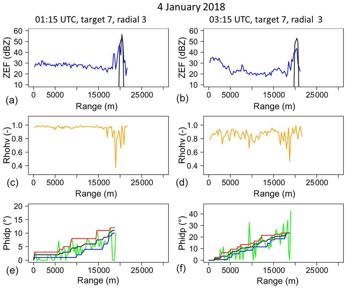
Figure 7Two examples (a, b) of Zh, ρhv, and ϕdp range profiles of the MOUC radar (0∘ PPI) during the 21 July 2017 convective event for one radial of a given mountain target. The raw horizontal reflectivity profiles (a, b) at the considered time steps (blue) are displayed together with the dry weather reference target value (black). The ρhv profiles (c, d) are used to detect the rainy gates not affected by clutter at close range and in the region of the mountain target. Panels (e) and (f) display the raw ψdp profiles (green) and the upper (red) and lower (blue) envelope curves and the regularized ϕdp profiles (black).
As representative examples, Fig. 7 illustrates the range profiles taken by the MOUC radar during the snowfall (left) and the ML (right) periods. As expected, the ρhv profiles are very different in the two cases, with ρhv values close to 1 in snow, indicating precipitation homogeneity while ρhv presents a high variability in the ML. During the ML period, we therefore had to adapt the ρhv threshold used to detect gates with precipitation. Based on the ρhv peak statistics presented by Khanal et al. (2019), we have chosen a value of 0.8. As it can be seen in Fig. 7, such a threshold may prevent the detection of the mountain reference return itself. Subsequently, we had to adapt the determination of ranges r0 and rM with respect to the XPORT radar case, firstly, by considering two successive gates corresponding to a range extent of 480 m (instead of 10 gates corresponding to 342 m) and, secondly, by making sure that the calculated rM value was less than the range of the first mountain reference gate. Regarding the regularization of the ψdp profiles (bottom graphs of Fig. 7), it was found that the raw profiles were noisier compared to the XPORT case study. Well-structured bumps were not evidenced in the ML profiles, maybe as a result of the lower-range resolution of the MOUC radar, and the regularization procedure was found to work satisfactorily. It remains, however, difficult to assume that there is no δhv contamination during the ML period.
Coming back to Fig. 6, one can note the mean value of ϕdp(rM) to be equal to 11.2∘ during the snowfall period, resulting in a specific differential phase shift on a propagation of 0.28∘ km−1 if the differential phase shift on backscatter is neglected. Such values indicate a significant heterogeneity in the horizontal and vertical dimensions of the snow/ice hydrometeors. During the rainy period between 04:10 and 06:00 UTC, there is good coherence between the specific attenuations derived from the MRT PIA (0.078 dB km−1 at around 04:00 UTC–0.035 dB km−1 at 06:00 UTC) and those derived from the polarimetry (0.076–0.046 dB km−1 at the same time steps) using the k–Kdp relationship established for this event and by using the DSD measurements available from the IGE site (see Sect. 3.3 below).
Our main objective with the 3–4 January 2018 event is to study the ϕdp–PIA relationship within the ML. Figure 6 indicates that both variables take, as expected, higher values during that period compared to during the snowfall and rainfall periods. The maximum values reached are 14.2 dB for PIAs and 25.6∘ for ϕdp(rM). Figure 6b and c also show that the cofluctuation of the two time series is not that good during the ML period, with a ϕdp(rM) signal having a trapezoidal shape with maximum values between 02:35 and 03:15 UTC, while the MRT PIA signal is more triangular and peaks at 03:15 UTC. We note that the two signals compare well after the peak, and that they both peak down at 03:55 UTC when measurements are made in the lowest part of the ML. These features are quite systematic for all of the 13 targets considered for the MOUC radar for this event, giving the impression that the ϕdp–PIA relationship depends on the position within the ML and, as such, on the physical processes occurring during the melting. This will be further illustrated and discussed in Sect. 4.2. However, we have to mention the following three points here that may limit the validity of such inferences for the MOUC radar configuration compared to the XPORT one: (i) the MRT PIA estimates may be positively biased by radome attenuation, (ii) the polarimetry-derived PIA estimates may be affected by δhv contamination in the ML, and (iii) nonuniform beam filling effects probably become significant for the 20–40 km range considered, leading to a smoothing of the radar signatures. There is no evidence so far of the first two points in the available dataset; this may be due to the moderate intensity of this precipitation event.
3.3 Study of the k–Kdp relationship in rain from in situ DSD measurements
Before presenting the analysis of the ϕdp–PIA relationship in rain and in the melting layer based on the estimates for all the mountain targets and time steps available for the two sets of events, we study in this subsection the k–Kdp relationships that we were able to derive from the DSD measurements collected at ground level at the IGE site. For all the events, precipitation was in the form of rainfall at this altitude. As for the scattering model, we used the CANTMAT version 1.2 software program that was developed at Colorado State University by Chenxiang Tang and Viswanathan N. Bringi. The raw Parsivel2 DSD measurements have a time resolution of 1 min. The volumetric concentrations were computed with a 5 min resolution and binned into 32 diameter classes with increasing sizes from 0.125 mm up to 6 mm. The CANTMAT software uses the T-matrix formulation to compute radar observables such as horizontal reflectivity, vertical reflectivity, differential reflectivity, copolar cross-correlation, specific attenuation, specific phase shift, etc., as a function of the DSD, the radar frequency, air temperature, oblateness models (e.g., Beard and Chuang, 1987; Andsager et al., 1999; Thurai and Bringi, 2005), and canting models for the rain drops and the incidence angle of the electromagnetic waves. Figure 8 displays the empirical k–Kdp pairs of points obtained for the convective events (left) and the stratiform one (right) as well as the fits of least square linear models and power law nonlinear regressions.
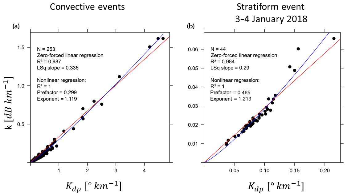
Figure 8DSD-derived k–Kdp relationships for the nine convective events (a) and for the stratiform event of 3–4 January 2018 (b) (see text for details).
Based on the literature review mentioning an almost linear relationship between k and Kdp at X band (Bringi and Chandrasekar, 2001; Testud et al., 2000; Schneebeli and Berne, 2012), we have first tested a linear regression with an intercept forced to be equal to 0 (red lines in Fig. 8). This simple model provides a rather good fit to the data, especially for the convective events. Due to the observed bending of the scatterplots, we have also tested a nonlinear regression to a power law model (blue curve) which significantly improves the fittings. A sensitivity analysis was performed in order to test the influence of the raindrop temperature, the raindrop oblateness model, the standard deviation of the canting angle distribution and the incidence angle. For reasonable ranges of the variation of these parameters, the DSD itself appears to be the most influential factor on the values of the regression coefficients. We note that the slopes of our zero-forced linear models are significantly higher than the values proposed in the literature (0.233 in Bringi and Chandrasekar, 2001; 0.205–0.245 in Scheebeli and Berne, 2012). The exponents of the fitted power law models are also significantly higher than 1.0. The fits in Fig. 8 correspond to the most likely parameterization of the scattering model in terms of temperature and incidence angles for the two events, i.e., 20 ∘C and 7.5∘, respectively, for the convective cases and 0 ∘C and 0∘ for the stratiform case. The Beard and Chuang (1987) formulation was used as the raindrop oblateness model. The DSD-derived linear and nonlinear k–Kdp relationships were used to process the regularized ϕdp(r) profiles which were first simply derived to obtain the Kdp(r) profiles prior to the application of the two k–Kdp relationships. The bottom graphs of Fig. 5 show examples of the resulting polarimetry-derived PIAs.
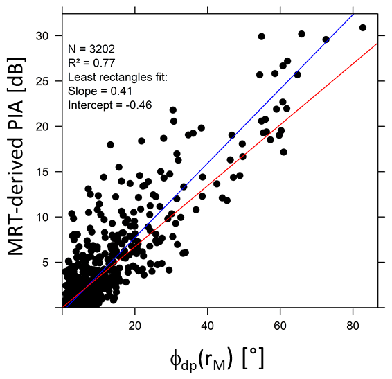
Figure 9PIA–ϕdp scatterplot for the nine convective events considered in this study. The blue line corresponds to the least rectangle fit to the data, while the red line corresponds to the linear k–Kdp relationship derived from the DSD data available at ground level.
4.1 Study of the ϕdp–PIA relationship in rain
Figure 9 displays the scatterplot of the ϕdp–PIA values obtained for the nine convective events (Table 2) with the XPORT 7.5∘ PPI data, following the methodology described in Sect. 3.1 and 3.2. The data from the 16 mountain targets (Table 3) were considered. For a given event, targets with maximum MRT-derived PIAs less than 5 dB were discarded in order to limit the weight of small PIA estimates in the global analysis. Since we consider the two variables to be on an equal footing, we preferred to calculate the least rectangles regression (blue straight line) between the two variables rather than the least squares regression of one variable over the other one. One can notice the rather large dispersion of the scatterplot with an explained variance of 77 %. We note the regression slope (0.41) to be higher than the slope of the k–Kdp linear relationship (0.336), which is reported as the red straight line in Fig. 9.
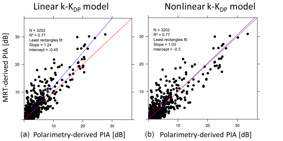
Figure 10Comparison of the PIAs derived from the mountain reference technique and from polarimetry using the linear k–Kdp relationship (a) and the nonlinear k–Kdp relationship (b) for the nine convective events. The blue line corresponds to the least rectangle fit to the data and the red line is the 1∕1 line.
To go further, Fig. 10 presents the comparison of the MRT-derived PIAs with the polarimetry-derived PIAs. The linear k–Kdp relationship leads to a significant positive bias for the polarimetry-derived PIAs with a least rectangles slope of 1.24. The nonlinear k–Kdp relationship does a good job of reducing this bias (least rectangles slope of 1.03). This result may be surprising given the k–Kdp relationships displayed in Fig. 8. One has to realize that the range of Kdp values is much smaller for the 5 min DSD estimations than for the Kdp(r) profiles discretized with a 34.2 m resolution. Considering that the 1 min DSDs allowed us to confirm the validity of the linear and nonlinear k–Kdp models for a wider Kdp range (not shown here for the sake of conciseness), we are therefore confident in the relevance of the results presented in Fig. 10.
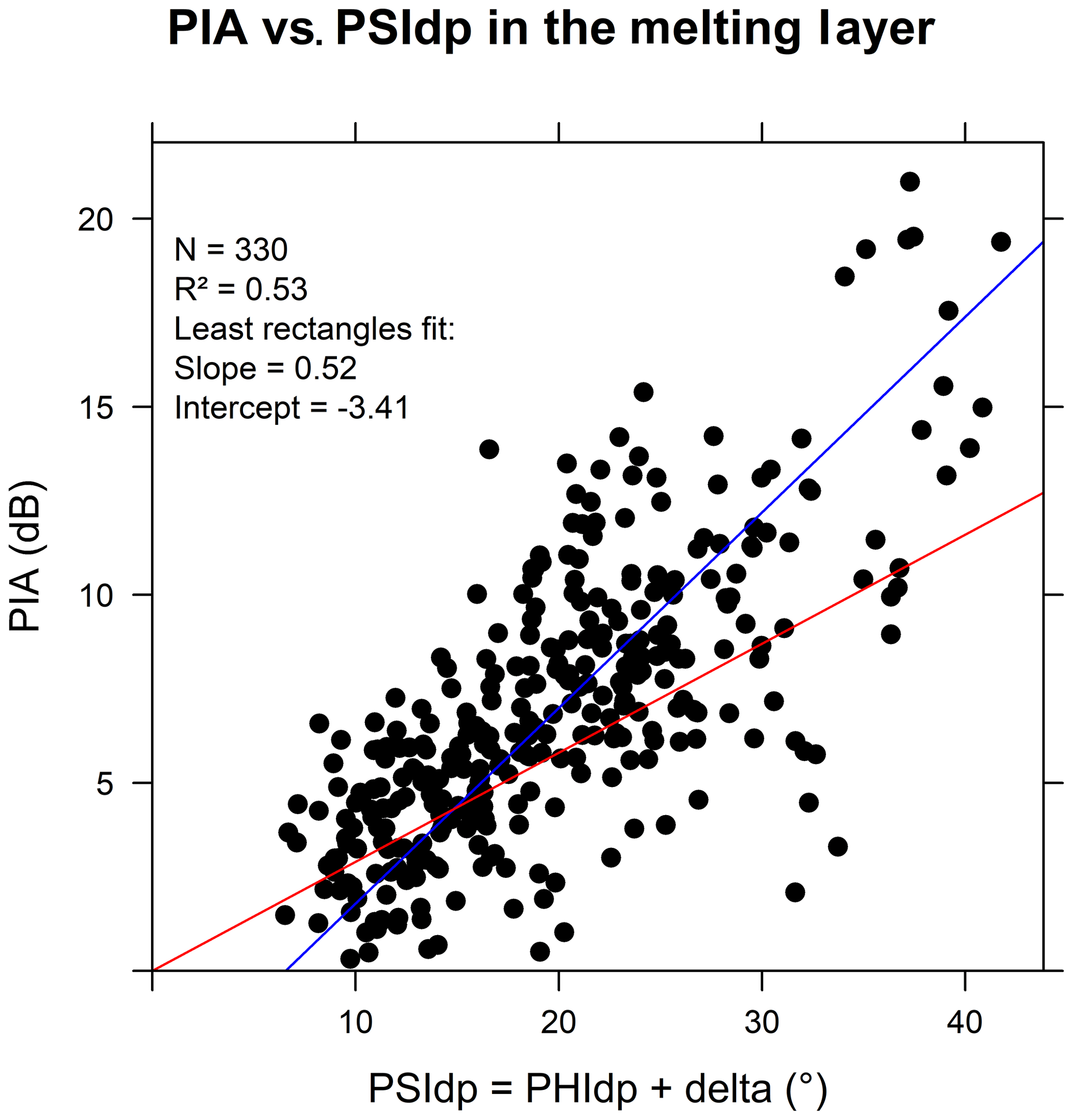
Figure 11PIA–ϕdp scatterplot in the ML for the stratiform event of 3–4 January 2018. The blue line corresponds to the least rectangle fit to the data, while the red line corresponds to the linear k–Kdp relationship derived from the DSD data available at ground level.
4.2 Study of the ψdp–PIA relationship in the melting layer
Figure 11 displays the scatterplot of the ϕdp–PIA values obtained in the ML for the 4 January 2018 stratiform event with the MOUC 0∘ PPI data, following the methodology described in Sect. 3.1 and 3.2. The results obtained for the 13 targets (Table 4) are considered in this analysis, with no target censoring based, for instance, on the minimum PIA observed for a given target as for the XPORT case study. One can see that the correlation between the two variables is severely degraded compared to the rain case with an explained variance of 41 % and a least rectangle slope of 0.51 dB per degree. The red line recalls the k–Kdp linear regression determined with the DSDs observed at ground level for this event. Clearly, the ϕdp–PIA relationship is different in rain and in the ML and, as suggested when commenting on Fig. 6, it likely depends on the physical processes occurring during the melting.
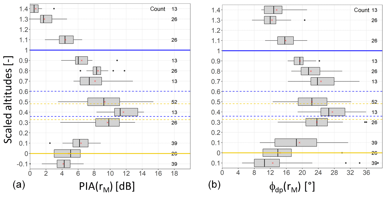
Figure 12Boxplots of the PIA and ϕdp values within the ML as a function of the scaled altitude (a and b, respectively) for the stratiform event of 4 January 2018. The horizontal blue and orange continuous lines represent the ML top and bottom, respectively; the broken horizontal blue and orange lines give the 10 % and 90 % quantiles of the scaled altitudes of the Zh and ρhv peak distributions, respectively.
To investigate this point, ϕdp(rM) and PIA(rM) values estimated during the rising of the ML at the level of the MOUC radar are represented in Fig. 12 as a function of their position within the ML. As already noted, we define the ML width as the difference between the Zh top altitude and the ρhv bottom altitude (Khanal et al., 2019). Since the ML width significantly varies during the considered period (from 630 to 1020 m; see Fig. 8), we found it necessary to scale the altitudes by the ML width. This was achieved by considering the following linear transformation of the altitudes:
where hM is the altitude (m a.s.l.) of the MOUC radar, hρhvB(t) is the altitude of the ML bottom and MLw(t) is the ML thickness at a given time t. The scaled altitude H(t) [–] subsequently takes the value 0 at ML bottom and the value 1 at ML top (orange and blue thick horizontal lines, respectively, in Fig. 12). Furthermore, in order to locate more precisely the position of the Zh and ρhv peaks within the ML, we computed their scaled altitudes at each time step, HzhP(t) and HρhvP(t), respectively, as follows:
and
where hzhP(t) and hρhvP(t) are the altitudes of Zh peak and ρhv peak at time t. The broken horizontal lines in Fig. 12 represent the 10 % and 90 % quantiles of the time series of the scaled altitudes of Zh peak (broken blue lines) and ρhv peak (broken orange lines). We can observe a shift between the Zh and ρhv characteristic altitudes, consistent with the ML climatology established by Khanal et al. (2019) who reported a shift of about 100 m in average between the two peaks. We note in Fig. 8 that this shift is visible during the snowfall period and at the beginning of the ML rising but that it is less pronounced after 03:00 UTC and during the rainfall period. In order to better evidence their vertical trends, the MRT PIA(rM) and ϕdp(rM) values are presented in Fig. 12 as a function of the scaled altitudes in the form of boxplots with a scaled altitude class of size 0.1. The number of counts in each class is indicated on the right of the graphs; it is a multiple of the number of MRT targets (13 here) depending on the time occurrence of estimates in a given altitude class. The vertical sampling is not very rich, with missing classes within the ML. However, there is a clear signature for the two variables in the ML. The trends already evoked when commenting on Fig. 8 are confirmed as follows: (i) the MRT PIAs peak when measurements are made at the level of the Zh and ρhv peaks – more precisely, the PIA peak is observed for the altitude class containing the ρhv peaks (scaled altitude class centered at 0.3); (ii) the region with maximum values is somewhat thicker for ϕdp, encompassing a significant part of the upper ML, between the 0.3 and 0.8 scaled altitude classes; (iii) ϕdp tends towards almost similar values on average in rain (ML bottom) and snow (ML top); and (iv) the PIA tends towards its value in rain below the ML and towards 0 above the ML. One would have expected a more pronounced return towards 0 of the PIAs on top of the ML. This lower-than-expected decrease could sign a radome attenuation; however, the rainfall intensity is low for the considered event, and the radome is equipped with a heating system so that accumulated snow is unlikely. It may also result from a smoothing effect related to nonuniform beam filling. With its 3 dB beamwidth of 1.28∘, the angular resolution of the measurements of the MOUC radar is 447 and 1005 m at distances of 20 and 45 km, respectively, which correspond to the minimum and maximum ranges of the considered mountain targets.
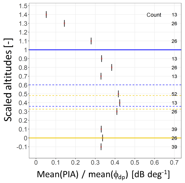
Figure 13Evolution of the ratio of the mean PIAs over the mean ψdp values within the ML as a function of the scaled altitudes for the stratiform event of 3–4 January 2018. The horizontal blue and orange lines represent the ML top and bottom, respectively; the broken horizontal blue and orange lines give the 10 % and 90 % quantiles of the scaled altitudes of the Zh and ρhv peak distributions, respectively.
Finally, Fig. 13 displays the evolution of the ratio of the mean of the MRT PIA(rM) values over the mean of ϕdp(rM) values as a function of the scaled altitudes. The value of the ratio below the ML (0.33) is in rather good agreement with the slope of the linear model established between the specific attenuation k and the specific differential phase shift Kdp using the DSD measurements in rain available for this event (0.29; see Fig. 9). Near the ρhv peak, the ratio value is equal to 0.42. For the three classes of scaled altitude 0.7, 0.8 and 0.9, the ratio is between 0.32 and 0.38, with an apparent secondary maximum for the altitude class 0.8. Data with increased vertical resolution would be necessary to confirm, or not, this observation, which is also visible on the PIA profile and on several ϕdp and PIA time series like the ones displayed in Fig. 8. Above the ML, the ratio progressively tends toward 0 at about 300 to 400 m.
In this work we developed a methodology for studying the relationship between total differential phase shift (ϕdp) and path-integrated attenuation (PIA) at X band. Knowledge of this relationship is critical for the implementation of attenuation corrections based on polarimetry. We used the mountain reference technique (MRT) for direct PIA estimations associated with the decrease in strong mountain returns during precipitation events. The MRT sensitivity depends on the time variability of the dry weather mountain returns. The MRT PIAs may be positively biased by on-site attenuation related in particular to radome attenuation and negatively biased by the effect of precipitation falling over the reference targets. The polarimetry PIA estimation is based on the regularization of the raw ψdp profiles, and their derivation in terms of specific differential phase shift (Kdp) profiles, followed by the application of a power law relationship between the specific attenuation and the specific differential phase shift. Such k–Kdp relationships were evaluated for rain with a scattering model by using DSD measurements and an oblateness model for raindrops. The noise of the raw ψdp profiles, the possible contamination of the signal by differential shift on backscatter and the adequacy of the k–Kdp relationship is the main factor that determines the quality of the polarimetry-derived PIAs. Nonuniform beam filling (NUBF) effects may also play a role. A point to emphasize is that both PIA estimators are not sensitive to an eventual radar miscalibration.
We presented first a rain case study based on nine convective events observed with the XPORT radar located in the Grenoble valley. A total of 16 mountain targets were considered with the dry weather mean apparent reflectivity greater than 45 dBZ. The stability of the apparent reflectivity of the mountain targets was shown to be very good, which is an indication of good radar calibration stability during the considered period. The time variability of the reference returns during dry weather preceding or succeeding the rain events was also found to be very small with standard deviations in the range of [0.2–0.9 dBZ], enabling a MRT PIA sensitivity better than 1 dB. Since the XPORT radar is radomeless, on-site attenuation effects are most likely negligible. The impact of rain falling over the mountain targets may also be very limited due to the high reflectivity threshold considered (45 dBZ). The development of the regularization procedure of the raw ψdp profiles required a significant effort, and we are confident in its ability to deal with the measurement noise, especially for heavy precipitation. We carefully examined many raw and regularized profiles, looking for possible evidence of δhv contamination during the considered convective events. We found some profiles with rather well organized bumps that could signal such contaminations. The regularization procedure was adapted in order to filter such effects, with a satisfactory performance when they occur at some distance (some kilometers) from the mountain target. In addition, we remind the reader that the observed ψdp(rM) values extend up to 80∘, while the theoretical δhv range is 0–4 dB. The δhv effect may therefore impact the results obtained only at the margin in the considered case study. NUBF effects may constitute an additional source of error which, although the rain events were convective, should remain limited due to the short ranges considered. In the end, the scatterplot of the MRT PIAs as a function of the ϕdp(rM) values for all the nine convective events presents a good coherence overall with, however, a significant dispersion (explained variance of 77 %). It is interesting to note that the nonlinear k–Kdp relationship derived from independent DSD measurements taken during the events of interest at ground level allows for a satisfactory transformation of the XPORT ϕdp(rM) values into almost unbiased (although dispersed) PIA estimates. Both estimation methods are prone to specific errors and, even if the MRT PIA estimator is more directly related to power attenuation, it is a priori difficult to say which estimator is the best. An assessment exercise of attenuation correction algorithms, making use of both PIA estimators, with respect to an independent data source (e.g., rain gauge measurements), is desirable to distinguish the two PIA estimators. From this perspective, a specific experiment is being designed within the RadAlp project and it will be implemented in the near future.
The melting layer (ML) case study of 3–4 January 2018 was made possible by the unique configuration of the observation system available. The study of the k–Kdp relationship within the ML is desirable to better quantify the attenuation effects in the ML with polarimetry; and one has to recognize that such a relationship can still be very difficult to characterize theoretically given that scattering models and particle size distributions need to be collected in the ML. The XPORT radar located at the bottom of the valley allowed for a detailed temporal tracking of the ML from below using quasi-vertical profiles derived from 25∘ PPIs. The MOUC radar provided horizontal scans at an altitude of 1917 m a.s.l. in the direction of several mountain targets during the rising of the ML in about 2 h. From this dataset, it was possible to derive the evolution of PIA(rM) and ϕdp(rM) values as a function of the altitude within the ML. The evolution with the altitude of the ratio of the mean value of PIA(rM) over the mean value of ϕdp(rM), as a proxy for the slope of a linear k–Kdp relationship within the ML, was also considered. Since the ML width varied during the ML rising, we found it necessary to scale the altitudes with respect to the ML width. The three variables considered present a clear signature as a function of the scaled altitude. In particular, the PIA∕ϕdp ratio peaks at the level of the ρhv peak (somewhat lower than the Zh peak), with a value of 0.42 dB per degree, while its value in rain just below the ML is 0.33 dB per degree. The latter value is consistent with the slope of the linear k–Kdp relationship (0.29) established from concomitant DSD measurements at ground level. The PIA∕ϕdp ratio remains quite strong in the upper part of the ML, between 0.32 and 0.38 dB per degree, before tending towards 0 above the ML. One would have expected a more pronounced return towards 0 of the PIAs on top of the ML. This lower-than-expected decrease could signal on-site attenuation occurring at the beginning of the ML rise due to the melting of the snow eventually accumulated over the radome; this effect is probably low for the considered event since the snowfall intensity was small and since the radome is heated. It may also result from a smoothing effect related to nonuniform beam filling (angular resolution of 447 and 1005 m for the range of mountain target distances). The δhv effect is likely to be strong in the ML (up to 4∘), and its relative importance may be quite high in our case study since the PIA range is significantly lower compared to the rain case study, with maximum PIAs of about 15 dB (note also that the sensitivity of the MRT is less than for the XPORT case study since the dry weather variability of the mountain returns is higher with standard deviations in the range [0.62–1.44]). However, we did not find evidence of δhv signatures in the raw ψdp(r) profiles, and we are confident in the ability of the regularization procedure to filter them in a rather satisfactory way if they eventually occur. Although the experimental configuration for the study of attenuation in the ML presents some limitations (e.g., possible radome attenuation and NUBF effects), the preliminary results presented here will be deepened by processing a dataset of about 30 stratiform events with the presence of the ML at the level of the MOUC radar.
Data can be made available by the first author upon request.
GD developed the concept of the article, realized the codes and performed the data processing; GD also wrote the article and handled the review process. AKK was involved in the development of the codes (ML identification, Phidp processing, etc.); NY shared his experience of the RHytMME radars and provided the MOUC radar data and the preliminary version of the Phidp regularization procedure. FC is a research engineer who has built the XPORT radar and is now responsible for the current updating program and the data acquisition. BB and NG contributed to the article through scientific discussions and amendments to the paper.
The authors declare that they have no conflict of interest.
We are grateful to Patrick N. Gatlin (NASA Marshall Space Flight Center, Huntsville, Alabama, USA) for providing the CANTMAT version 1.2 software developed at Colorado State University by Chenxiang Tang and Viswanathan N. Bringi, whom we also thank. The RadAlp experiment is cofunded by the LabEX OSUG@2020 of the Observatoire des Sciences de l'Univers de Grenoble, the Service Central Hydrométéorologique et d'Appui à la Prévision des Inondations (SCHAPI) and Electricité de France/Division Technique Générale (EDF/DTG).
This paper was edited by Gianfranco Vulpiani and reviewed by three anonymous referees.
Anagnostou, E. N., Anagnostou, M. N., Krajewski, W. F., Kruger, A., and Miriovsky, B. J.: High-Resolution Rainfall Estimation from X-Band Polarimetric Radar Measurements, J. Hydrometeor., 5, 110–128, https://doi.org/10.1175/1525-7541(2004)005<0110:HREFXP>2.0.CO;2, 2004.
Andsager, K., Beard, K. V., and Laird, N. E.: Laboratory measurements of axis ratios for large raindrops, J. Atmos. Sci., 56, 2673–2683, https://doi.org/10.1175/1520-0469(1999)056<2673:LMOARF>2.0.CO;2, 1999.
Beard, K. V. and Chuang, C.: A new model for the equilibrium shape of raindrops, J. Atmos. Sci., 44, 1509–1524, https://doi.org/10.1175/1520-0469(1987)044<1509:ANMFTE>2.0.CO;2, 1987.
Bouilloud, L., Delrieu, G., Boudevillain, B., Borga, M., and Zanon, F.: Radar rainfall estimation for the post-event analysis of a Slovenian flash-flood case: application of the Mountain Reference Technique at C-band frequency, Hydrol. Earth Syst. Sci., 13, 1349–1360, https://doi.org/10.5194/hess-13-1349-2009, 2009.
Bringi, V. N. and Chandrasekar, V.: Polarimetric Doppler weather radar, principles and applications, Cambridge University Press, 636 pp., 2001.
Delrieu, G., Caoudal, S., and Creutin, J. D.: Feasibility of using mountain return for the correction of ground-based X-band weather radar data, J. Atmos. Ocean. Tech., 14, 368–385, https://doi.org/10.1175/1520-0426(1997)014<0368:FOUMRF>2.0.CO;2, 1997.
Delrieu, G., Serrar, S., Guardo, E., and Creutin, J. D.: Rain Measurement in Hilly Terrain with X-Band Weather Radar Systems: Accuracy of Path-Integrated Attenuation Estimates Derived from Mountain Returns, J. Atmos. Ocean. Tech., 16, 405–416, https://doi.org/10.1175/1520-0426(1999)016<0405:RMIHTW>2.0.CO;2, 1999.
Delrieu, G., Andrieu, H., and Creutin, J. D.: Quantification of path-integrated attenuation for X- and C-band weather radar systems operating in Mediterranean heavy rainfall, J. Appl. Meteor., 39, 840–850, https://doi.org/10.1175/1520-0450(2000)039{%}3C0840:QOPIAF{%}3E2.0.CO;2, 2000.
Diss, S., Testud, J., Lavabre, J., Ribstein, P., Moreau, E., and Parent du Chatelet, J.: Ability of a dual polarized X-band radar to estimate rainfall, Adv. Water Resour., 32, 975–985, https://doi.org/10.1016/j.advwatres.2009.01.004, 2009.
Foresti, L., Sideris, I. V., Panziera, L., Nerini, D., and Germann, U.: A 10-year radar-based analysis of orographic precipitation growth and decay patterns over the Swiss Alpine region, Q. J. Roy. Meteor. Soc., 144, 2277–2301, https://doi.org/10.1002/qj.3364, 2018.
Germann, U., Galli, G., Boscacci, M., and Bolliger, M.: Radar precipitation measurement in a mountainous region, Q. J. Roy. Meteor. Soc., 132, 1669–1692, https://doi.org/10.1256/qj.05.190, 2006.
Joss, J. and Lee, R.: The Application of Radar-Gauge Comparisons to Operational Precipitation Profile Corrections, J. Appl. Meteor., 34, 2612–2630, https://doi.org/10.1175/1520-0450(1995)034<2612:TAORCT>2.0.CO;2, 1995.
Khanal, A. K., Delrieu, G., Cazenave, F., and Boudevillain, B.: Radar remote sensing of precipitation in high mountains: detection and characterization of Melting Layer in French Alps, Atmosphere, 10, 784, https://doi.org/10.3390/atmos10120784, 2019.
Koffi, A. K., Gosset, M., Zahiri, E.-P., Ochou, A. D., Kacou, M., Cazenave, F., and Assamoi, P.: Evaluation of X-band polarimetric radar estimation of rainfall and rain drop size distribution parameters in West Africa, Atmos. Res., 143, 438–461, https://doi.org/10.1016/j.atmosres.2014.03.009, 2014.
Marzoug, M. and Amayenc, P.: A class of single and dual-frequency algorithms for rain-rate profiling from a spaceborne radar: Part 1 – Principle and tests from numerical simulations, J. Atmos. Ocean. Tech., 11, 1480–1506, https://doi.org/10.1175/1520-0426(1994)011{%}3C1480:ACOSAD{%}3E2.0.CO;2, 1994.
Matrosov, S. Y. and Clark, K. A.: X-Band Polarimetric Radar Measurements of Rainfall, J. Appl. Meteor., 41, 941–952, https://doi.org/10.1175/1520-0450(2002)041{%}3C0941:XBPRMO{%}3E2.0.CO;2, 2002.
Matrosov, S. Y., Kingsmill, D. E., Martner, B. E., and Ralph, F. M.: The Utility of X-Band Polarimetric Radar for Quantitative Estimates of Rainfall Parameters, J. Hydrometeor., 6, 248–262, https://doi.org/10.1175/JHM424.1, 2005.
Matrosov, S. Y., Campbell, C., Kingsmill, D. E., and Sukovich, E.: Assessing Snowfall Rates from X-Band Radar Re?ectivity Measurements, J. Atmos. Ocean. Tech., 26, 2324–2339, https://doi.org/10.1175/2009JTECHA1238.1, 2009.
Otto, T. and Russchenberg, H. W. J.: Estimation of Specific Differential Phase and Differential Backscatter Phase From Polarimetric Weather Radar Measurements of Rain, IEEE Geosci. Remote S., 8, 988–992, https://doi.org/10.1109/LGRS.2011.2145354, 2011.
Ryzhkov, A. V., Giangrande, S. E., and Schuur, T. J.: Rainfall estimation with a polarimetric prototype of WSR-88D, J. Appl. Meteor., 44, 502–515, https://doi.org/10.1175/JAM2213.1, 2005.
Ryzhkov, A. V., Diederich, M., Zhang, P., and Simmer, C.: Potential utilization of specific attenuation for rainfall estimation, mitigation of partial beam blockage and radar networking, J. Atmos. Ocean. Tech., 31, 599–619, https://doi.org/10.1175/JTECH-D-13-00038.1, 2014.
Ryzhkov, A., Zhang, P., Reeves, H., Kumjian, M., Tschallener, T., Trömel, S., and Simmer, C.: Quasi-Vertical Profiles – A new way to look at polarimetric radar data, J. Atmos. Ocean. Tech., 33, 551–562, https://doi.org/10.1175/JTECH-D-15-0020.1, 2016.
Schneebeli, M. and Berne, A.: An Extended Kalman Filter Framework for Polarimetric X-Band Weather Radar Data Processing, J. Atmos. Ocean. Tech., 29, 711–730, https://doi.org/10.1175/JTECH-D-10-05053.1, 2012.
Serrar, S., Delrieu, G., Creutin, J. D., and Uijlenhoet, R.: Mountain Reference Technique: Use of mountain returns to calibrate weather radars operating at attenuating wavelengths, J. Geophys. Res.-Atmos., 105, 2281–2290, https://doi.org/10.1029/1999JD901025, 2000.
Sideris, I. V., Gabella, M., Erdin, R., and Germann, U.: Real-time radar–raingauge merging using spatio-temporal co-kriging with external drift in the alpine terrain of Switzerland, Q. J. Roy. Meteor. Soc., 140, 1097–1111, https://doi.org/10.1002/qj.2188, 2014.
Testud, J., Le Bouar, E., Obligis, E., and Ali-Mehenni, M.: The Rain Profiling Algorithm Applied to Polarimetric Weather Radar, J. Atmos. Ocean. Tech., 17, 332–356, https://doi.org/10.1175/1520-0426(2000)017{%}3C0332:TRPAAT{%}3E2.0.CO;2, 2000.
Thurai, M. and Bringi, V. N.: Drop axis ratios from 2D video disdrometer, J. Atmos. Ocean. Tech., 22, 963–975, https://doi.org/10.1175/JTECH1767.1, 2005.
Trömel, S., Kumjian, M. R., Ryzhkov, A. V., Simmer, C., and Diederich, M.: Backscatter differential phase – estimation and variability, J. Appl. Meteor. Climatol., 52, 2529–2548, https://doi.org/10.1175/JAMC-D-13-0124.1, 2013.
Westrelin, S., Meriaux, P., Tabary, P., and Aubert, Y.: Hydrometeorological risks in Mediterranean mountainous areas – RHYTMME Project: Risk Management based on a Radar Network. ERAD 2012 7th European Conference on Radar in Meteorology and Hydrology, June 2012, Toulouse, France. 6 p., hal-01511157, 2012.
Yu, N. and Gaussiat, N.: A monotonic algorithm for estimation of the specific differential phase. Poster presentation during the 10th European Conference on Radar in Meteorology and Hydrology (ERAD 2018), 1–6 July 2018, Ede-Wageningen, the Netherlands, 2018.
Yu, N., Gaussiat, N., and Tabary, P.: Polarimetric X-band weather radars for quantitative precipitation estimation in mountainous regions, Q. J. Roy. Meteor. Soc., 144, 2603–2619, https://doi.org/10.1002/qj.3366, 2018.