Retrieval of lower-order moments of the drop size distribution using CSU-CHILL X-band polarimetric radar: a case study

The lower-order moments of the drop size distribution (DSD) have generally been considered difficult to retrieve accurately from polarimetric radar data because these data are related to higher-order moments. For example, the 4.6th moment is associated with a specific differential phase and the 6th moment with reflectivity and ratio of high-order moments with differential reflectivity. Thus, conventionally, the emphasis has been to estimate rain rate (3.67th moment) or parameters of the exponential or gamma distribution for the DSD. Many double-moment “bulk” microphysical schemes predict the total number concentration (the 0th moment of the DSD, or M₀) and the mixing ratio (or equivalently, the 3rd moment M₃). Thus, it is difficult to compare the model outputs directly with polarimetric radar observations or, given the model outputs, forward model the radar observables. This article describes the use of double-moment normalization of DSDs and the resulting stable intrinsic shape that can be fitted by the generalized gamma (G-G) distribution. The two reference moments are M₃ and M₆, which are shown to be retrievable using the X-band radar reflectivity, differential reflectivity, and specific attenuation (from the iterative correction of measured reflectivity Z_h using the total Φ_dp constraint, i.e., the iterative ZPHI method). Along with the climatological shape parameters of the G-G fit to the scaled/normalized DSDs, the lower-order moments are then retrieved more accurately than possible hitherto. The importance of measuring the complete DSD from 0.1 mm onwards is emphasized using, in our case, an optical array probe with 50 µm resolution collocated with a two-dimensional video disdrometer with about 170 µm resolution. This avoids small drop truncation and hence the accurate calculation of lower-order moments. A case study of a complex multi-cell storm which traversed an instrumented site near the CSU-CHILL radar is described for which the moments were retrieved from radar and compared with directly computed moments from the complete spectrum measurements using the aforementioned two disdrometers. Our detailed validation analysis of the radar-retrieved moments showed relative bias of the moments M₀ through M₂ was <15 % in magnitude, with Pearson’s correlation coefficient >0.9. Both radar measurement and parameterization errors were estimated rigorously. We show that the temporal variation of the radar-retrieved mass-weighted mean diameter with M₀ resulted in coherent “time tracks” that can potentially lead to studies of precipitation evolution that have not been possible so far.

1 Introduction

The principal application of polarimetric radar has historically been directed towards more accurate estimation of rain rate (R) that is driven largely by the operational agencies for hydrological applications. It now strongly appears that, as a major step forward, the operational algorithm for the US Weather Surveillance Radar – 1988 Doppler (WSR-88D) network will be based on specific attenuation because, among other advantages, it is linearly related to rain rate at S-band (Ryzhkov et al., 2014; Cocks et al., 2019; Wang et al., 2019). This method has also been evaluated quite extensively at X-band by Diederich et al. (2015), where the specific attenuation (A_h) is much larger than at S-band but not linear with R. The development of R(A_h) algorithms rests on a large body of work since the early 1990s and is related to attenuation correction using the differential propagation phase as a constraint (Bringi et al., 1990; Smyth and Illingworth, 1998; Testud et al., 2000; Bringi and Chandrasekar, 2001, and references therein).

The retrieval of drop size distribution (DSD) parameters has also been a strong impetus for radar polarimetry. In this context, there exists a large body of literature that is based mainly on the unnormalized (Ulbrich, 1983) or normalized (Illingworth and Blackman, 2002; Testud et al., 2001) gamma model. This model is parameterized by a set of three quantities, namely $\mathit{\{}{N}_{\mathrm{0}},\mathit{\mu },\mathrm{\Lambda }\mathit{\}}$ or $\mathit{\{}{N}_{\mathrm{w}},\mathit{\mu },D_{\mathrm{m}}\mathit{\}}$, where N₀ and N_w are “intercept” parameters, μ is the shape factor, Λ is the “slope”, D_m is the ratio of the 4th to 3rd moments of the DSD N(D), and D is the diameter of the raindrop (Ryzhkov and Zrnić, 2019, and references therein). The gamma model has also been used in the double-moment “bulk” microphysical schemes that predict the mass mixing ratio (or equivalently the 3rd moment M₃; for moment order k, we write M_k and the total concentration of drops (or M₀) (e.g., Meyers et al., 1997). The lower-order moments of the DSD (M₀ through M_3+b, where b is the exponent of the fall-speed-D power law), are important in describing various microphysical processes such as collisional (break-up and coalescence), evaporation, and sedimentation (e.g., Milbrandt and Yau, 2005). However, radar polarimetry has not been focused on these lower-order moment retrievals because the radar observables (horizontal) reflectivity Z_h, differential reflectivity Z_dr, and specific differential phase K_dp are related to the higher-order moments such as M₆, the ratio M₇∕M₆, and M_4.5, respectively.

Defining a scaled diameter $x=D/D_{\mathrm{m}}$, the normalized DSD is a function of x as $h\left(x\right)=N\left(D\right)/N_{\mathrm{w}}$. The observation of Testud et al. (2001) regarding the “remarkable” stability of the shape of h(x) using measured DSDs was a significant advance because they did not impose an a priori form for h(x). Apart from the shape “stability” of h(x), they also showed a large compression in the “scatter” of h(x) compared to N(D). While they did not refer to their normalization as double-moment using M₃ and M₄ as the reference moments, Lee et al. (2004, henceforth, L04) generalized the scaling/normalization framework by introducing any two reference moments M_i and M_j of any order i, j>0. As per this framework, in a compact notation, $N\left(D\right)=N_{\mathrm{0}}^{\prime }h\left(x\right)$ with a different $x=D/D_{\mathrm{m}}^{\prime }$, where $N_{\mathrm{0}}^{\prime }=M_i^{(j+\mathrm{1})/(j-i)}{M}_j^{(i+\mathrm{1})/(i-j)}$ and $D_{\mathrm{m}}^{\prime }$ is the ratio of $(M_j/M_i{)}^{\mathrm{1}/(j-i)}$. In essence, the variance of the DSDs due to different rain types and intensities is largely controlled by the variability in $N_{\mathrm{0}}^{\prime }$ and $D_{\mathrm{m}}^{\prime }$ and much less so by h(x). Further, any moment M_k can be expressed as power laws of M_i, M_j, in which the coefficient is the kth moment of h(x) and the two exponents are predetermined by i and j. L04 also recognized that if h(x) is assumed to follow the generalized gamma (G-G) model with two shape parameters, then it could fit most naturally occurring DSD shapes. We refer the reader to Stacy (1962) for the expressions of the probability density function (pdf) of the G-G and its moments. The G-G form has been applied to model cloud droplet spectra, ice crystal and snow spectra (Delanoë et al., 2014), as well as raindrop spectra (Raupach and Berne, 2017a; Thurai and Bringi, 2018). The three-moment normalization for this model is provided in Szyrmer et al. (2005). The generalization to K-moment normalization scheme given in Morrison et al. (2019) does not specify any particular form for h(x) other than that its moments should be finite. In agreement with Szyrmer et al. (2005), they found that three-moment normalization was sufficient to “compress” the scatter of h(x). Further, it minimized the errors in the estimation of the other moments expressed as power laws of the reference moments. For remote-sensing applications (cloud and drizzle), they found that the set of moments $\mathit{\{}{M}_{\mathrm{2}},M_{\mathrm{3}},M_{\mathrm{6}}\mathit{\}}$ was one possible choice mentioning lidar backscatter (M₂), microwave attenuation (M₃), and radar reflectivity (M₆). While the combination of M₃ and M₆ was not optimal for estimating the lower-order moments (in particular, M₀), it was better than using M₆ alone.

Recently, using the double-moment approach of L04, Raupach and Berne (2017a, RBa) showed that measured DSDs in stratiform rain with h(x) expressed in the G-G form have shape factors that are sufficiently “invariant” for practical use across different rain climatologies if the reference moments are chosen carefully. Their result essentially validated the “remarkable” stability conclusion of h(x) by Testud et al. (2001) which was based on limited data in oceanic rain. RBa speculated that the transition (i.e., between convective and stratiform rain) and convective rain DSDs would also have a sufficiently “invariant” h(x), but they did not have a large enough database to make such a conclusion.

The polarimetric (X-band) radar retrieval of moments using reference moments M₃ and M₆ and an “invariant” h(x) of the G-G form were first described in Raupach and Berne (2017b, RBb). Their retrieval of M₆ was based on Z_h, while M₃ was retrieved in a two-step procedure using Z_dr and K_dp. We discuss their results in detail later in this paper. Here, it suffices to mention that their measured DSDs were based on a network of Parsivel disdrometers, which did not have the resolution to measure the shape of h(x) for D<0.75 mm or so (as shown later by Raupach et al., 2019). Additionally, with “noisy” Z_dr and K_dp radar data (for Z_h<37 dBZ), their validation of the moments (M₀ through M₇) using radar measurements was not conclusive but was sufficient to demonstrate that their approach gave results similar to other methods based on the normalized gamma model using “more classical” radar retrievals of $\mathit{\{}{N}_{\mathrm{w}},\mathit{\mu },D_{\mathrm{m}}\mathit{\}}$ (Gorgucci et al., 2008; Kalogiros et al., 2012).

Whereas RBb used measured DSDs and the polarimetric radar forward operator to derive the retrieval algorithms for M₃ and M₆, there has been a reverse moment-based polarimetric forward operator (Kumjian et al., 2019). This reverse approach employs a very large database of measured and bin-resolved one-dimensional (1-D) model output DSDs to build a look-up table that maps the various moment pairs to the expected values of Z_h, Z_dr, and K_dp along with their standard deviations. Their application was to determine the moment pairs that could potentially be prognosed in numerical microphysical schemes of rain would be “optimally” constrained by polarimetric radar measurements. They found that the pair {M₆,M₉} was optimal in terms of lowest variability in $\mathit{\{}{Z}_{\mathrm{h}},Z_{\mathrm{dr}},K_{\mathrm{dp}}\mathit{\}}$ but that the pair {M₃,M₆} was suboptimal but still “useable”. Thus, RBb’s choice of {M₃,M₆} as the two reference moments was validated by Kumjian et al. (2019). The rationale through which M₉ (whose sampling error would be very large using available disdrometers) entered the moment pair is not entirely clear. It could be because of correlating Z_dr with absolute moments (M₀ through M₉) as opposed to the more physically based ratio of moments such as $D_{\mathrm{m}}^{\prime }=(M_{\mathrm{6}}/M_{\mathrm{3}}{)}^{\mathrm{1}/\mathrm{3}}$ in RBb or M₇∕M₆ as in Jameson (1983).

This work further develops on RBb but, instead of K_dp, we employ specific attenuation (A_h) given its operational use in estimating R. The iterative correction of measured reflectivity Z_h using the total Φ_dp constraint, i.e., the iterative ZPHI algorithm, which is a variant of Testud et al. (2000), is used here to estimate A_h (Bringi et al., 2001; Park et al., 2005a, b). The reference moment M₃, which is proportional to rain water content (W), is retrieved using a modification of Jameson (1993) by fitting A_h∕W as a smoothed cubic spline with D_m. The prior step is the retrieval of $D_{\mathrm{m}}^{\prime }$ from Z_dr and then the retrieval of D_m from $D_{\mathrm{m}}^{\prime }$. This multi-step procedure was found to minimize the parameterization errors (also referred to as algorithm errors) in the estimation of M₃. As in RBb, the reference moment M₆ is derived as power-law fit to Z_h. The other major difference with RBb is the use of collocated optical array probe (50 µm resolution) and two-dimensional video disdrometer (2DVD) inside a double-fence wind shield (Thurai et al., 2017a). The “complete” DSD was measured from 0.1 mm onwards thus avoiding truncation at the small drop end. This leads to more accurate estimates of the lower-order moments as well as more accurate h(x). The methodology of G-G fits to h(x) are described in Thurai and Bringi (2018) and Raupach et al. (2019). The use of a very narrow (0.33^∘) beam at X-band with high gain and a short vertical distance from radar pixel to the instrumented site were additional factors that differed from RBb. We also show coherent “time tracks” in the D_m versus M₀, D_m versus W, and $D_{\mathrm{m}}^{\prime }$ versus M₆ planes, where all variables are based on radar retrievals.

The rest of the article is organized as follows. In the next section, we briefly discuss the surface instrumentation (disdrometers). The CSU-CHILL radar and its use in characterizing the multi-cell storm complex (the case study) as well as data extracted over the instrumented site are given in Sect. 3. The retrieval of the two reference moments {M₃,M₆} follows in Sect. 4. Several different ways of validating the moment retrievals are presented in Sect. 5. We follow this with a discussion in Sect. 6 and summarize the case study in Sect. 7. We cannot draw firm conclusions from just one case study even though the analysis is quite detailed. Rather this work may be considered a proof-of-concept that will require further validation to be undertaken in the future. It is difficult to find radar data with revisit times <90 s over an instrumented site unless a dedicated experiment is proposed and funded. In our case, the event of 23 May 2015 was largely a target of opportunity as one of the co-authors (PCK) had the foresight to collect data on this day without considering that it would lead to a detailed case study of moment retrievals. An Appendix provides procedures for estimating the radar measurement error contribution to the variances of, firstly, the reference moments {M₃,M₆}, and then the variances of the other moments. The estimates of the variances of the ratio of correlated variables of the form X^pY^−q are derived using a Taylor expansion to second order. The parameterization error variances are estimated for {M₃,M₆} and summed with the radar measurement error variances to yield the total error variance for each moment retrieved.

Throughout this paper, we use “H” as a subscript for reflectivity Z_H to denote units of dBZ at horizontal polarization. The lower case “h” in Z_h means units of mm⁶ m⁻³. The same applies to Z_DR (in dB) or Z_dr (ratio). The functions Var(⋅) and $\stackrel{\mathrm{‾}}{(\cdot )}$ yield the variance and mean of their arguments, respectively. We use Cov(X,Y) for the covariance between the variables X and Y. A set is denoted by curly brackets $\mathit{\{}\cdot ,\cdot ,\cdot \mathit{\}}$. The notation 𝔼{⋅} is used for the statistical expectation; 〈⋅〉 for the average of its argument; Γ(⋅) for the gamma function; and 𝕀m{⋅} for the imaginary part of its complex argument.

2 Surface instrumentation

The principal surface-based instruments used in this study are the MPS (or Meteorological Particle Spectrometer, manufactured by Droplet Measurement Technologies) and third-generation 2DVD, both located within a 2∕3-scale Double Fence Intercomparison Reference (DFIR; Rasmussen et al., 2012) wind shield. As reported in Notaroš et al. (2016), the 2∕3-scale DFIR was effective in reducing the ambient wind speeds by nearly a factor of 3 based on data from outside and inside the fence. An OTT Pluvio rain gage was also available for rain rate and rain accumulation comparison with the disdrometers.

Our retrieval algorithms (see Sect. 4) of the reference moments M₃ and M₆ were based on scattering simulations from the combined DSD data from two sites, namely Greeley, Colorado (GXY), and Huntsville, Alabama (HSV). The same disdrometer and wind shield configuration were deployed at both locations. However, the case study in this paper concerns the event of 23 May 2015 captured in Greeley, which also has a coincident CHILL X-band radar. Huntsville has a very different climate from Greeley, and its altitude is 212 m mean sea level (m.s.l.) as compared with 1.4 km m.s.l. for Greeley. According to the Köppen–Trewartha climate classification system (Trewartha and Horn, 1980), Greeley has a semiarid-type climate, whereas Huntsville has a humid subtropical-type climate (Belda et al., 2014).

The MPS is an optical array probe (OAP) that uses the technique introduced by Knollenberg (1970, 1976, 1981) and measures drop diameter in the range from 0.05 to 3.1 mm (but the upper end of the usable range is limited to 1.5 mm due to reduced sampling volume). A 64-element photo-diode array is illuminated with a 660 nm collimated laser beam. Droplets passing through the laser cast a shadow on the array, and the decrease in light intensity on the diodes is monitored with the signal processing electronics. A two-dimensional image is captured by recording the light level of each diode during the period that the array is shadowed. The limitations and uncertainties associated with OAP measurements have been well documented (Korolev et al., 1991, 1998; Baumgardner et al., 2017). The sizing and fall speed errors primarily depend on the digitization error (±25 µ). The fall speed accuracy according to the manufacturer (DMT) is <10 % for 0.25 mm and <1 % for sizes greater than 1 mm, limited primarily by the accuracy in droplet sizing. To calculate N(D), the measured fall speed is not used. Rather a cubic polynomial fit from the manufacturer (DMT) is employed. Details of the calculation of N(D) are given in the Appendix of Thurai et al. (2017a) and updated in Raupach et al. (2019).

The third-generation 2DVD is described in detail by Bernauer et al. (2015). Its operational characteristics are similar to earlier generations. In particular, the accuracy of size and fall speed measurement has been well documented (e.g., Schönhuber et al., 2007, 2008; Thurai et al., 2007, 2009; Huang et al., 2008). Considering the horizontal pixel resolution of about 170 µm and other factors, the effective sizing range is D>0.7 mm (Thurai et al., 2017a). The fall velocity accuracy is determined primarily by the accuracy of calibrating the distance between the two orthogonal light “sheets” or planes and is <5 % for fall velocity <10 m s⁻¹ (Schönhuber et al., 2008). A comparison of fall speeds between the MPS and 2DVD has been reported by Bringi et al. (2018) from both the GXY and HSV sites, with excellent agreement. The only fall velocity threshold used for the 2DVD is the lower limit set at 0.5 m s⁻¹ in accordance with the manufacturer guidelines for rain measurements. The instrument is designed to prevent drops from entering the housing where the cameras are positioned. Without going into details, it suffices to mention that small drops can enter via slits that allow the light to illuminate the cameras, or drops can hang on the slits. Both of these effects cause spurious images that the matching software cannot reject (Larsen and Schönhuber, 2018). Thus, caution is necessary when using the 2DVD fall speeds for sizes <0.6 mm (about 3–4 pixels).

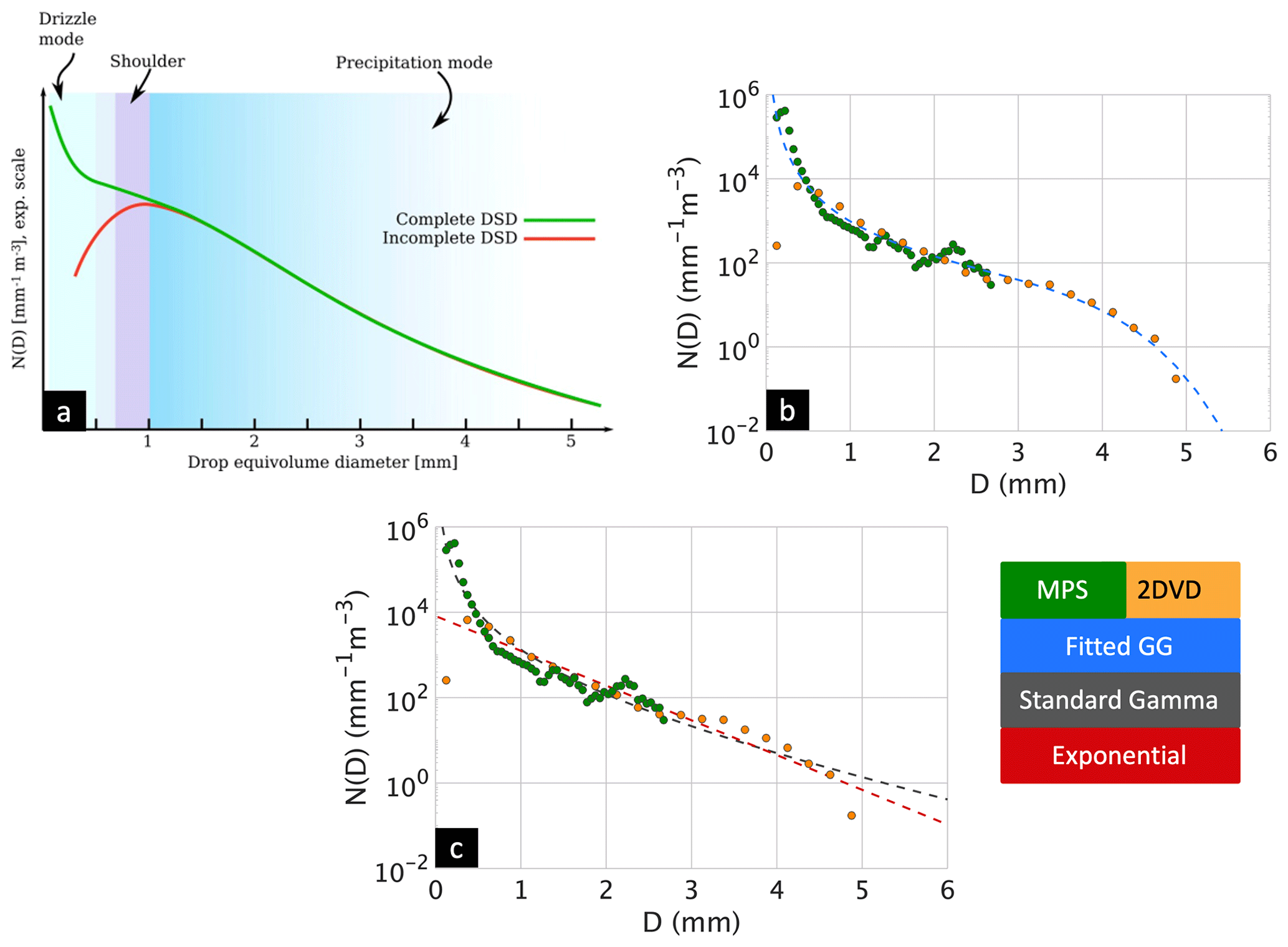
Figure 1 (a) Conceptual illustration of the complete DSD comprising the drizzle mode, the “shoulder” region, and the precipitation mode. The incomplete DSD is due to drop truncation by instruments that cannot measure the concentration of small drops. (b) An example of measured 3 min averaged DSD (R≈60 mm h⁻¹) using a collocated optical array probe with a 2DVD showing the separate measurements (note the high resolution of the MPS and the drop truncation of the 2DVD). The composite or compete spectrum is obtained by using the MPS for D≤0.75 mm and 2DVD for D>0.75 mm. The dashed blue line is the G-G fit (with parameters $\mathit{\mu }=-\mathrm{0.3}$, c=6; see Eq. (1) for details) to the complete spectrum. Data from the 23 May 2015 case study at 20:45 UTC. (c) Same data points as panel (b) but with the standard gamma (black) and exponential (red) fits.

In our application, we utilize the MPS for measurement of small drops with $\mathrm{0.1}\le D<\mathrm{0.75}$ mm and the 2DVD for larger-sized drops (see Raupach et al., 2019 for the rationale). This is termed here the “complete” size spectrum, and 2928 3 min averaged spectra were available from the two sites with a minimum rain rate of 0.1 mm h⁻¹ and a maximum of 286 mm h⁻¹. More details of the rainfall types, measurement time periods, comparison with gages, and related analyses are available in Thurai et al. (2017a) and Raupach et al. (2019). Figure 1a illustrates the “complete” DSD with the “drizzle” mode defined by a peak in N(D) occurring when D<0.5 mm (Abel and Boutle, 2012). The “shoulder” is the diameter range where the N(D) either remains steady or falls off more “slowly” (generally found under equilibrium conditions: McFarquhar, 2004). The precipitation range is used here for larger-sized drops after the “shoulder”, if any. These ranges are used here only to illustrate Fig. 1. The “incomplete” spectra, in which small drops are not measured accurately due to resolution, sensitivity, or other issues (2DVD or Parsivel; Park et al., 2017), frequently show the convex down shape at the small drop end. Here, we only use the complete N(D) by compositing the data from MPS and 2DVD. An example is shown in Fig. 1b, which illustrates the main features of the “complete” DSD during the time that peak rain rate (3 min averaged R of 60 mm h⁻¹) was occurring at the instrumented site during the 23 May 2015 event. We refer the reader to the following link for further details: http://www.chill.colostate.edu/w/DPWX/Modeling_observed_drop_size_distributions:_23_May_2015 (last access: 27 August 2020). The shape is equilibrium-like but with a single “drizzle” mode, a well-defined shoulder, and faster (than exponential) fall-off in the tail (Low and List, 1982; McFarquhar, 2004; Straub et al., 2010). These features cannot be captured by either standard gamma or exponential fits, as shown in Fig. 1c.

3 CSU-CHILL radar

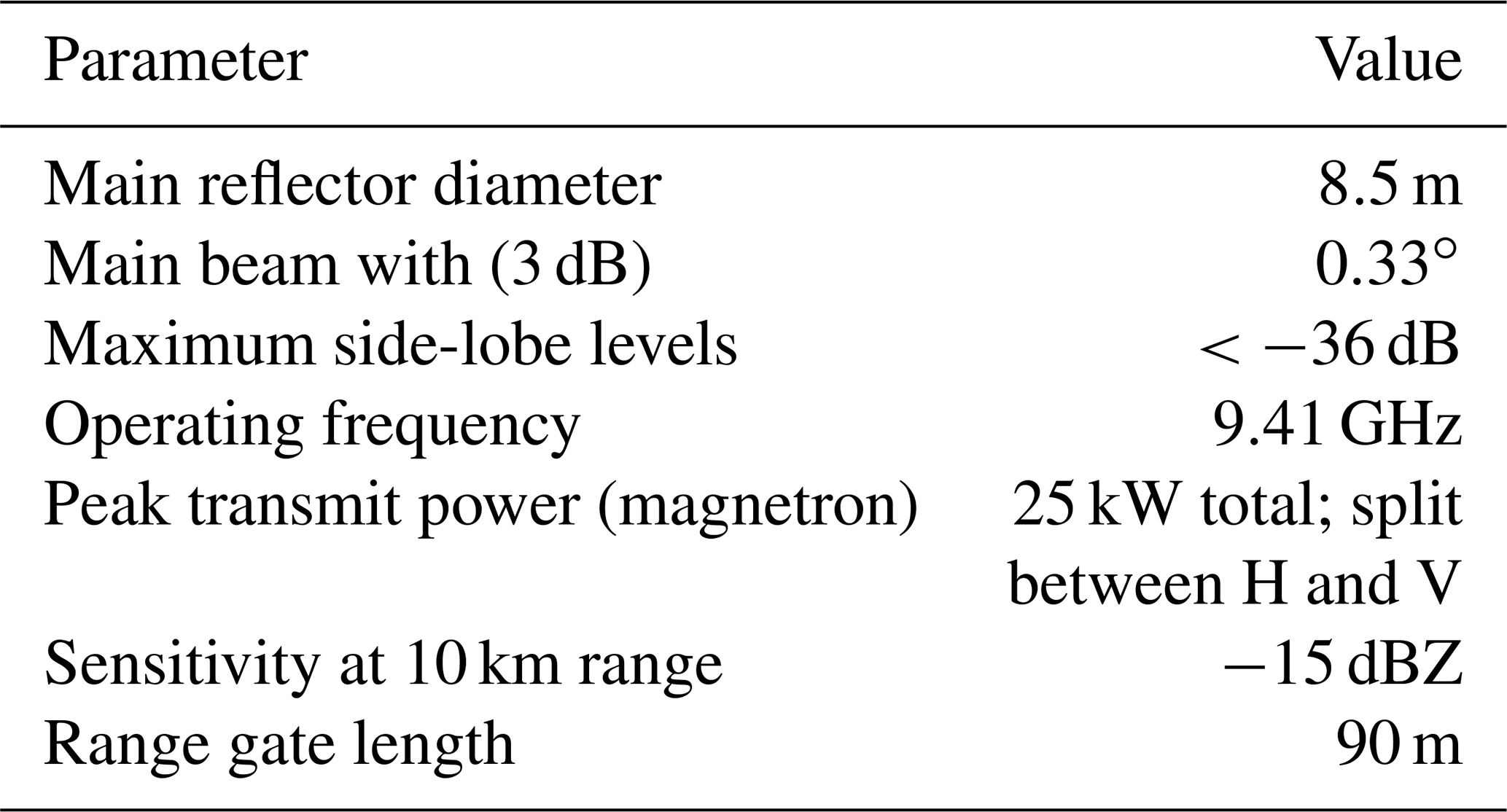
The CSU-CHILL (Colorado State University-University of Chicago/Illinois State Water Survey) radar is described in Brunkow et al. (2000) and Bringi et al. (2011a). Details on the conversion to a dual-wavelength system and the current radar specifications are given in Junyent et al. (2015) (see the condensed version in Table 1).

Suffice to state here that the X-band polarimetric mode is “simultaneous transmit and receive” or SHV and the 3 dB beam width is very narrow at 0.33^∘ with a gain of 55 dB. There are three separate feed or orthogonal mode transducers (OMTs) available: (a) an S-band feed (beam width in the far field is 1^∘) whose performance is described in Bringi et al. (2011a), (b) an S–X-band dual-wavelength feed that was used in the data described herein, and (c) an X-band feed. For the 23 May 2015 event, our retrievals of the reference moments {M₃,M₆} are based on the X-band polarimetric data $\mathit{\{}{Z}_{\mathrm{h}},Z_{\mathrm{dr}},{\mathrm{\Phi }}_{\mathrm{dp}}\mathit{\}}$ only, where Φ_dp is differential phase shift. Only X-band data were used even though S-band data were available simultaneously. Our choice for using the X-band data was due to the very high resolution provided by the 0.33^∘ beam and the larger range of values for the X-band specific attenuation for a given rain rate (relative to S-band). The case study convective event was a complex of multiple cells with strong azimuthal and elevation gradients across the “echo cores” which generally precludes accurate dual-wavelength estimation of range-resolved specific attenuation. The narrow X-band beam also allows a lower elevation angle (1.5^∘) to be used before clutter contaminates the signal. The instrumented site was located at Easton, which is 13 km SSE of the radar (along the 171.25^∘ azimuth). Details of the terrain variation between the radar and the Easton site are given in Kennedy et al. (2018).

Table 1 Technical specifications of the CSU-CHILL X-band channel with the dual-offset Gregorian antenna.

3.1 Brief description of storm characteristics from radar

The synoptic environment on 23 May 2015 was conducive to thunderstorm development in northeastern Colorado. A low at the 500 hPa level was analyzed over Utah at 12:00 UTC. This system was forecast to move eastward and promote upward motion within the moist air mass that was in place over the eastern plains of Colorado. In recognition of this situation, the Storm Prediction Center (SPC) Convective Outlook valid for the afternoon hours included a slight risk of severe thunderstorm development over northeastern Colorado. Persistent low cloud coverage ended up limiting surface heating within ∼50 km of CSU-CHILL, reducing thunderstorm intensity. The SPC storm reports did not contain any severe category hail (diameter of 2.54 cm or larger) or surface wind speeds of 25 m s⁻¹ or more. Volunteer weather observers reported several instances of small (0.64 cm or less) hail mostly in the Rocky Mountain foothills ∼60 km southwest of the radar. Afternoon surface temperatures were ∼14 ^∘C in the CSU-CHILL/Greeley area. The 0 ^∘C level in the Denver late afternoon sounding was at ∼3.5 km m.s.l. (2.1 km above ground level – a.g.l.).

Figure 2 shows a low elevation angle (1.5^∘) plan position indicator (PPI) scan of S-band Z_H at 20:45 UTC which was the time of peak rainfall at the instrumented site (also referred to as Easton) identified by the + marker in Fig. 2. The main echo feature is the near N–S orientation of multiple 55 dBZ cores extending from the Easton site to nearly 50 km to the south. The rainfall over the site lasted for over 90 min, and PPI scans at a fixed 1.5^∘ elevation angle were repeated every 90 s. This good time resolution enabled the validation of the moment retrievals which otherwise would not have been possible (for example, with WSR-88D scan cycle times of around 5 min).

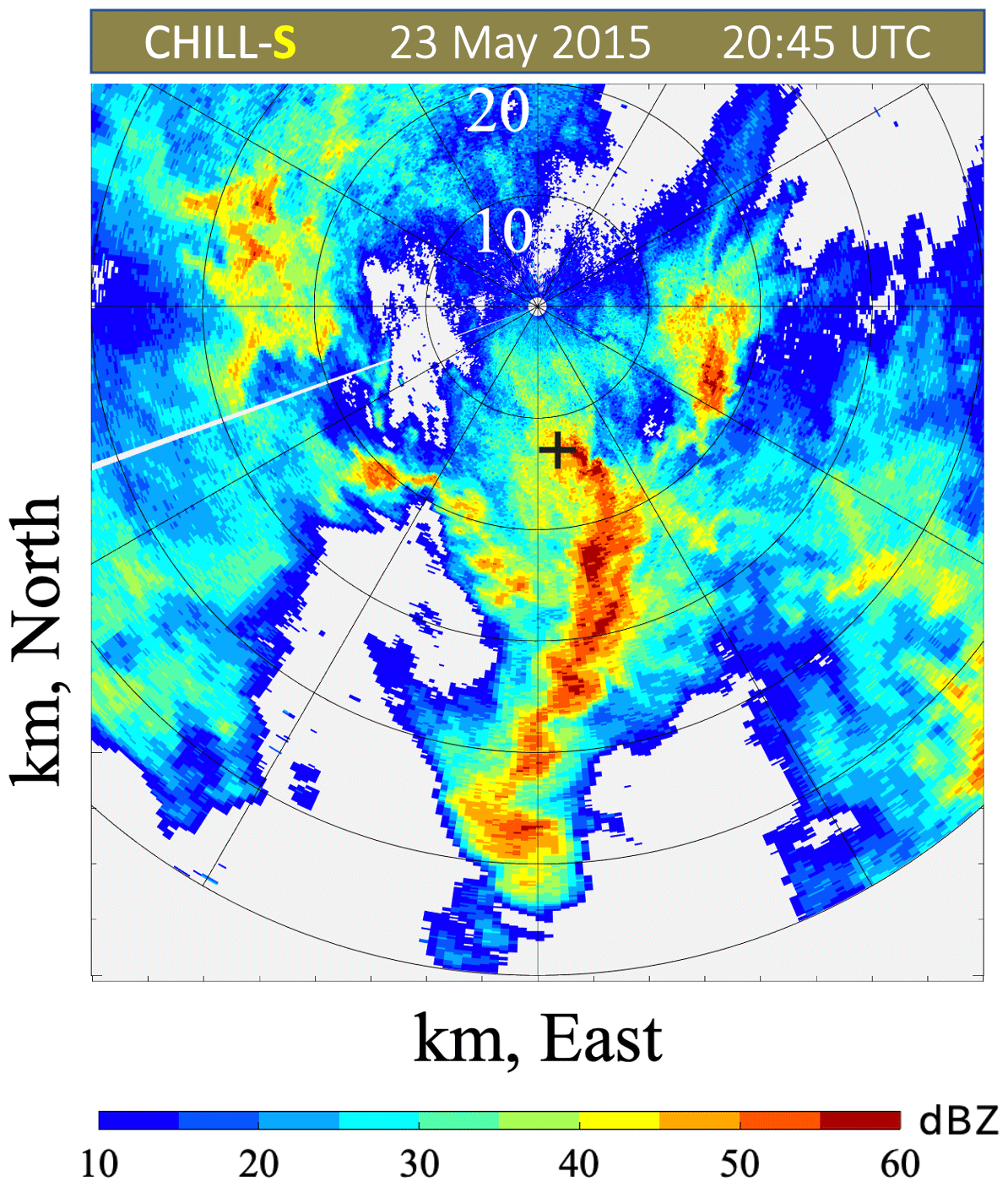
Figure 2 Low elevation angle (1.5^∘) PPI sweep of S-band reflectivity (Z_H) at 20:45 UTC. The “+” marks the location of the instrumented site (MPS and 2DVD).

The general echo movement near Easton was estimated at 10 m s⁻¹ towards the radar on average from the south. After the peak echo of 55 dBZ traversed the instrumented site, another cell produced very heavy rain at the radar site with no evidence of graupel/hail (visual observations by one of the co-authors, PCK). One volunteer observer located 15 km east of the Easton instrumentation site reported 0.64 cm hail mixed with heavy rain between 20:30 and 20:45 UTC. The CSU-CHILL radar data showed that this small hail was generated by an isolated, higher-reflectivity cell that was separated from the storms that crossed the instrumented site. We do not believe that hail occurred at the Easton site during the analyzed time period, as also confirmed by 2DVD fall speed observations.

There was no range–height indicator (RHI) scan at 20:45 UTC. Therefore, the vertical echo structure could not be determined at this time close to the peak rainfall over Easton, but RHI scans about 18 min earlier performed along the 171^∘ azimuth are shown in Fig. 3. The top panel shows measured reflectivity at the X-band (uncorrected for attenuation), while the measured S-band reflectivity is plotted in the bottom panel. Several strong cells (>55 dBZ) are noted south of Easton at ranges of 27 and 32 km; the cell at 32 km shows significant attenuation. However, there is no significant attenuation at the 13 km range where the instrumented site is located. The 10 dBZ echo top reaches 8 km a.g.l.

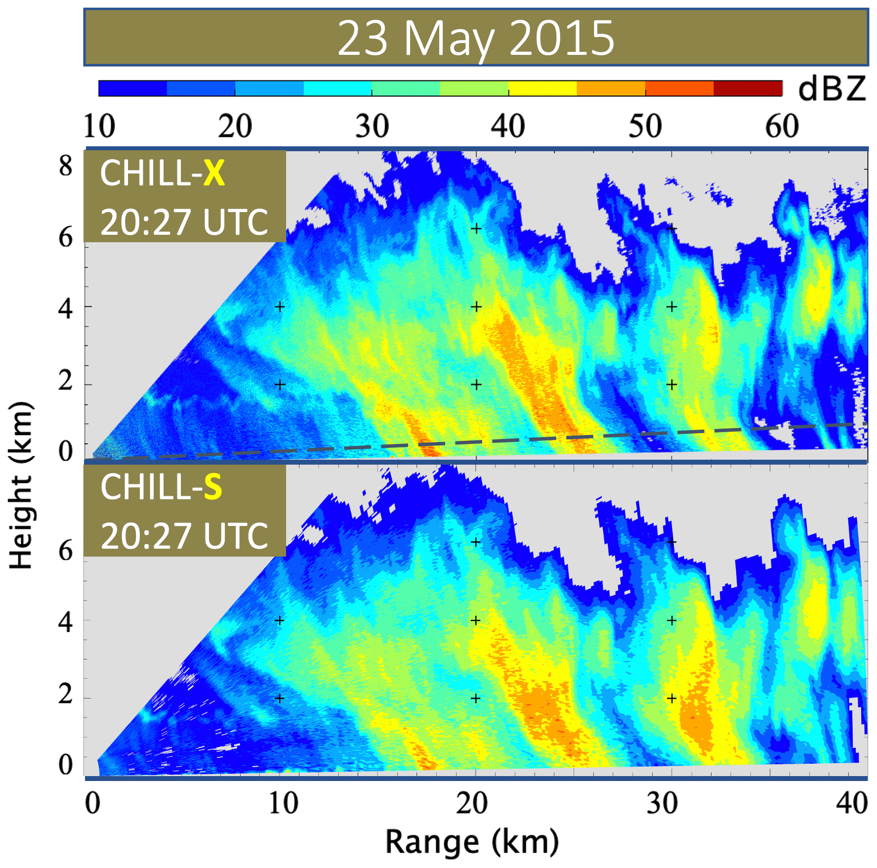
Figure 3 RHI sweep of Z_H along the 171^∘ azimuth at 20:27 UTC about 18 min before peak echo descended on the Easton instrumented site at a range of 13 km. The “+” marks are at 2 km intervals. (Top) X-band measured (uncorrected) reflectivity. The range profiles of radar data along the dashed line are shown in Fig. 4. (Bottom) S-band measured reflectivity.

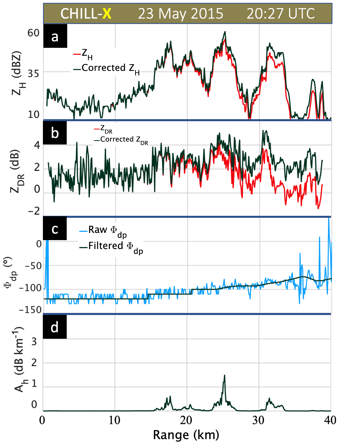
Figure 4 (a) Range profiles of measured and attenuation-corrected Z_H at X-band at 20:27 UTC at an azimuth angle of 171^∘ (elevation angle of 2^∘). The Easton instrumented site is located at a range of 13 km, (b) measured and attenuation-corrected Z_DR at X-band, (c) measured and filtered Φ_dp, and (d) specific attenuation (A_h).

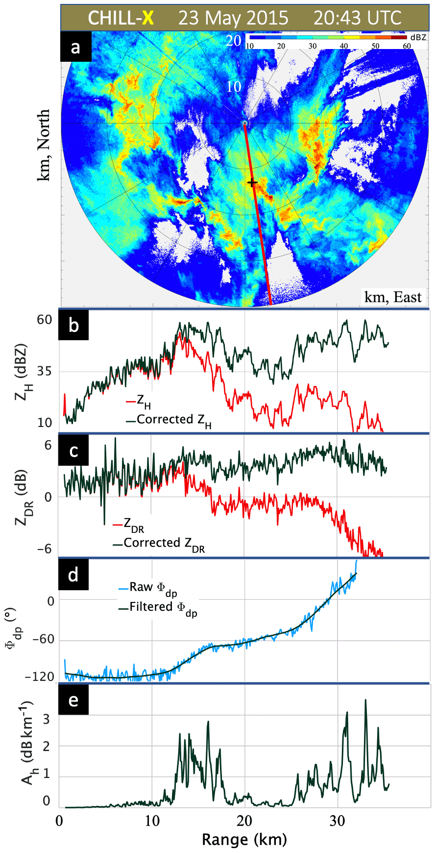
Figure 5 (a) PPI of measured X-band reflectivity at 20:43 UTC (elevation angle is 1.5^∘). The range profiles in the panels below are along the red line (radial) to the instrumented site denoted by the “+” marker. (b)–(e) As in Fig. 4, panels (a)–(d), except at 20:43 UTC.

3.2 Attenuation correction

As mentioned earlier, we use the X-band radar for quantitative moment retrievals. It is apparent that the strong cells will cause attenuation, so the X-band measured Z_h and Z_dr have to be corrected for attenuation and differential attenuation, respectively. The method used herein is exactly the same as described in Mishra et al. (2016). To correct the measured Z_h, we apply an iterative version of the ZPHI method, which uses a Φ_dp constraint (Testud et al., 2000; Bringi et al., 2001) that was originally developed at C-band but later extended to X-band by Park et al. (2005a, b). In short, the coefficient α in the linear relation between the specific attenuation at H polarization (A_h) and specific differential phase (K_dp) is determined by minimizing a cost function based on least squares (we refer to Bringi and Chandrasekar, 2001, for details), whereas the standard ZPHI method uses a fixed a priori value for α (Testud et al., 2000). In addition, a power law of the form $A_{\mathrm{h}}=b_{\mathrm{2}}{Z}_{\mathrm{h}}^{b_{\mathrm{1}}}$ is assumed where b₁=0.78 and b₂ are constants (Park et al., 2005a). The method gives the estimate of A_h at each resolution volume in the selected range interval (here 0–40 km). The upshot of using A_h instead of K_dp is that the former closely follows the variations in Z_h without the smoothing needed for estimating the latter but with all the advantages of K_dp such as immunity to calibration offsets and partial beam blockage (Ryzhkov et al., 2014). Note that using A_h for retrieval of W is restricted to precipitation comprising pure rain. In contrast, using K_dp (as in RBb) in pure rain entails spatial (range) smoothing which, in compact convective rain cells, “distorts” the spatial representation of the rain rate profile depicted by Z_H. In our multi-step retrieval procedure, it is reasonable not to mix different smoothing scales for the radar observables. There are many variants of the attenuation-correction method at X-band, as elucidated, for example, by Anagnostou et al. (2004) and Gorgucci and Chandrasekar (2005). Here, the iterative filtering method of Hubbert and Bringi (1995) is used to separate the backscatter differential phase from the propagation phase. In essence, the estimate of A_h may be considered a by-product of attenuation correction of the measured Z_h using the differential propagation phase over the selected path interval as a constraint.

The correction of the measured Z_dr for differential attenuation is based on an extension of the method proposed by Smyth and Illingworth (1998) for C-band, which is described in Bringi and Chandrasekar (2001) as a “combined Φ_dp-Z_dr” constraint. The extension to X-band is described in Park et al. (2005b), which is used herein with some modifications implemented for the CSU-CHILL radar. In brief, the A_h determined by the Φ_dp constraint is scaled by a factor ν and the measured Z_dr is corrected for differential attenuation (A_dp=νA_h) such that a desired value is reached at the end of the beam. The desired value is the intrinsic or “true” Z_dr at the end of the beam, which is estimated from the corrected Z_h using a mean Z_h–Z_dr relation based on scattering simulations that use measured DSDs from several locations that encompass a wide variety of rain types. This sets a constraint for Z_dr at the end of the beam (generally Z_dr≈0 dB because of light rain at the end of the beam or because of ice particles above the 0 ^∘C level). By the end of the beam, we mean the last range gate where the hydrometer echoes are detected. Range profiles of measured and corrected Z_H and Z_DR, the measured and filtered Φ_dp (which is used as constraints from 0 to 40 km), and A_h are shown in the four panels of Fig. 4 at 20:27 UTC along the radial to the instrumented site located at Easton. The Z_H profiles show that very minor attenuation correction is needed at this time, while the Z_DR is corrected by 2 dB at the end of the ray. The change in differential phase, i.e., ΔΦ_dp, is also small at 25^∘. Consistent with these values, the A_h peak is 1.5 dB km⁻¹, coinciding with the Z_H peak at 25 km. At the Easton location (13 km range) the A_h is negligible.

Figure 5a shows the PPI (at an elevation angle of 1.5^∘) of the measured X-band Z_H at 20:43 UTC, at which time the peak 55 dBZ echo traversed over the instrumented site. The X-band reflectivity in Fig. 5a can be compared with S-band data in Fig. 2. The line of cells organized south of the radar causes significant attenuation of the X-band signal power. This is clear in the range profile in Fig. 5b, where the attenuation has increased dramatically with Z_H corrected by 35 dB and Z_DR by 9 dB. The ΔΦ_dp now increases by around 150^∘. Assuming a nominal α of 0.25^∘ km⁻¹, the path-integrated attenuation would be 37.5 dB. The A_h values have increased with peaks of 3 dB km⁻¹. At the Easton site, A_h≈1.5 dB km⁻¹. From a moment-retrieval viewpoint, significant attenuation correction only begins beyond the Easton site (13 km range), so that the errors due to such correction will not be significant in this case. This situation persists after 20:43 UTC until the end of the analysis period (21:35 UTC or so).

3.3 Time series of radar measurements and DSD-based simulations

A “necessary” condition for accurate radar retrievals of DSD moments is that the time series of corrected Z_h, Z_dr, K_dp, and A_h extracted over the resolution volumes (or pixels) surrounding the Easton site agree “reasonably” well with the same observables simulated using measured DSDs and a scattering model (what is generally referred to as the forward radar model/operator). The criterion of “reasonable” agreement is difficult to quantify but is elucidated in Thurai et al. (2012) using error variance separation. The radar data were extracted around a polar area defined by a range interval ±0.18 km centered at the range (13 km) to Easton and ±0.2^∘ in azimuth angle for a total of 15 pixels surrounding the Easton site. The height of the pixels at an elevation angle of 1.5^∘ at the 13 km range is 340 m a.g.l. The radar data from each pixel are plotted as a time series in Fig. 6 which shows the pixel-to-pixel variability. A Lee (1980) filter (henceforth Lee filter) used to reduce speckle in images is adapted here to filter the pixel-to-pixel variability with a sliding window of ±11 (weighted) points; the filtered values are shown in Fig. 6 interpolated in time to that of the disdrometer. The “effective” time resolution after Lee filtering is 2.5 min. The radar time series were shifted backward in time by 60 s, as is common when matching the peak in Z_h (e.g., May et al., 1999). A more general analysis of the error characterization of radar–gage comparison is given in Anagnostou et al. (1999). However, such an analysis is not needed herein because of the narrow antenna beam and short range to the instrumented site. Thurai et al. (2012) applied the Lee filter to time-series data versus range filtering applied to range gates along a fixed ray profile and showed that they were nearly equivalent. The Lee-filtered values of the radar data show the time evolution of the main echo passage over the Easton site.

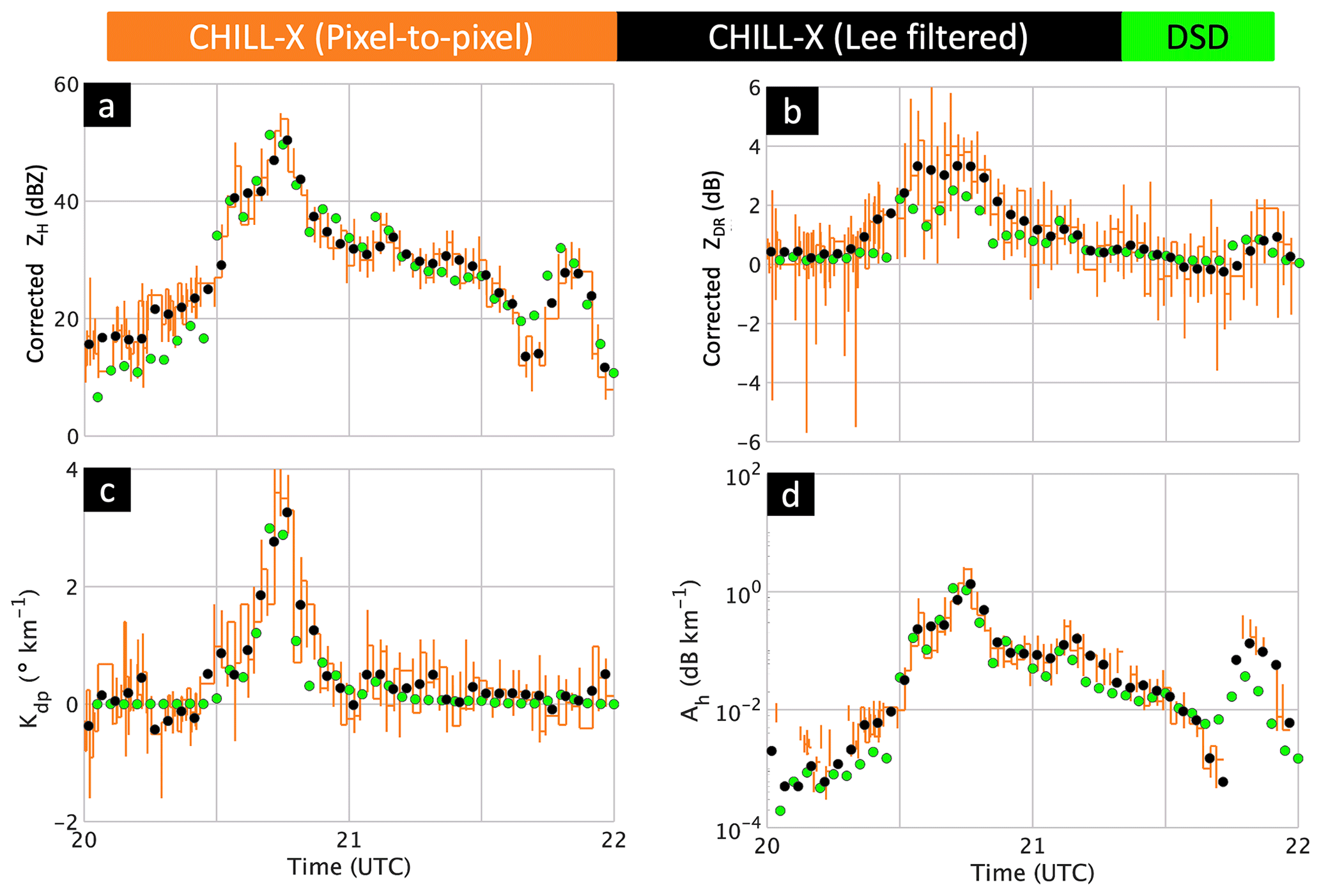
Figure 6 Time series of X-band radar data compared with simulations based on measured complete DSDs and the scattering model described in the text. (a) Corrected Z_H from radar showing pixel-to-pixel variations which have been filtered using Lee (1980). (b–d) Same but, respectively, for corrected Z_DR, K_dp, and A_h.

The composite 3 min averaged DSDs (an example was shown in Fig. 1b) were used to simulate radar observables as a time series using the T-matrix scattering code (Barber and Yeh, 1975; Bringi and Seliga, 1977). The time resolution of 3 min corresponds to a spatial scale of 1.8 km (using an echo movement speed of 10 m s⁻¹), which is less than the echo cell sizes estimated to be around 2–3 km. For an estimate of the decorrelation time of radar-retrieved D₀, we refer the reader to Thurai et al. (2012), who studied stratiform rain with embedded weak convection using 4 s samples; the 1∕e-folding time was around 200 s, where e is Napier's constant. For a highly convective case of our present case study, the decorrelation time would be substantially smaller but probably similar to our radar sampling of 90 s. Further, in Bringi et al. (2015), the decorrelation distance in a highly convective squall line event was estimated to be 3.5 km for radar-retrieved R; the time resolution obtained using a radar sampling time of 40 s was 2.5 min. In our case, the echo speed of 10 m s⁻¹ together with the “effective” Lee-filtered radar resolution of 2.5 min and the disdrometer 3 min averaging corresponds to spatial distances in the range 1.5–1.8 km. This is well within the estimated 1∕e-decorrelation distance of 3.5 km in Bringi et al. (2015).

While the DSD data were available at much higher time resolution, the choice of 3 min averaged DSD is a compromise between smaller DSD sample sizes when integration times are, say, 1 min, versus poorer representativeness of the spatial scales for longer time integrations (e.g., 5 min). The radar update time was around 90 s, which is short enough not to introduce excessive temporal representativeness errors. Note that in Fig. 6a, the DSD-based simulated Z_H is about 5 dB lower than that measured by radar for the time period 20:00–20:30 UTC. The measured Z_H was 18–25 dBZ, implying very low rain rates (∼0.5 mmh⁻¹) and a low number density of drops sampled by the disdrometers. In addition, it follows from the RHI taken at 20:27 UTC in Fig. 3 that the cells are moderately slanted from NNW aloft, where generating cells might have formed at 5 km a.g.l. to SSE at the surface. Given the unsteady conditions in this complex of echoes, it is not surprising that the disdrometer-based Z_H calculation is biased low by around 5 dB relative to low radar Z_H values of 18–25 dBZ. These problems are mitigated when heavier rain rates traverse the site about 15 min later.

The scattering model is based on the mean shapes from the 80 m fall bridge experiment described in Thurai et al. (2007) and Gaussian canting angle distribution with mean = 0^∘ and standard deviation σ=7^∘ (from Huang et al., 2008). The dielectric constant of water at a wavelength of 3 cm and a temperature of 8 ^∘C (Ray, 1972) was used. The time series of the simulated radar observables are shown in Fig. 6 marked as “DSD”. The visual agreement between simulations and the Lee-filtered mean radar values are qualitatively quite good except for a small underestimation of simulated Z_dr relative to radar measurements by around 0.5 dB at $\sim \mathrm{20}:\mathrm{45}$ UTC. The discrepancy at 21:40 UTC noted in Fig. 6a and d is because of heavy rain on radome (observed by PCK). Overall, the good agreement between corrected radar measurements and the DSD-based forward simulations shows good calibration of Z_h and Z_dr. The radar-retrieved specific attenuation closely follows the Z_h due to the A_h–Z_h power-law assumption in the ZPHI method (only the fixed exponent is relevant), whereas the K_dp does not, as expected.

4 The methodology of radar retrieval of the DSD moments

As mentioned in Sect. 1, the methodology we used here follows RBb except for the use of specific attenuation rather than K_dp in the retrieval of M₃ (however, both methods use Z_dr in a multi-step retrieval described below). There are several advantages to this approach. First, “noisy” A_h is strictly positive, as opposed to K_dp, which can be “noisy” with both positive- and negative-valued fluctuations in measurements. This is an issue because horizontal orientation of raindrops is usually assumed for simulation of K_dp from DSD measurements, meaning that all simulated K_dp values used to train retrieval algorithms are positive. Second, the smoothing in range necessary for K_dp is not needed for A_h, which closely follows the spatial variability in Z_h. The basis for the retrieval methodology lies in the double-moment normalization of L04. This method is explained in detail in RBb and, hence, we only summarize it in the next subsection.

4.1 Overview

Moment retrievals from polarimetric radar data are a relatively recent application of the scaling/normalization of the DSD. There are several aspects in this scaling as described by L04, namely that there is substantial reduction in the scatter in h(x) from the un-normalized scatter, implying that most of the variability of the DSD can be attributed to variability in $N_{\mathrm{0}}^{\prime }$ and $D_{\mathrm{m}}^{\prime }$, with h(x) being relatively “stable” with varying rain types/intensities. There is considerable latitude in the choice of reference moments {M_i,M_j} in the double-moment scheme depending on the application with $N_{\mathrm{0}}^{\prime }$ expressed as $M_i^{(j+\mathrm{1})/(j-i)}{M}_j^{(i+\mathrm{1})/(i-j)}$ and $D_{\mathrm{m}}^{\prime }$ as a ratio of $(M_j/M_i{)}^{\mathrm{1}/(j-i)}$. Further, any moment M_k can be expressed as power laws of M_i, M_j, and the kth moment of h(x). RBa showed that the amount of variance in individual DSD moments captured by the normalization scheme depends on the choice of reference moments.

RBb first suggested the use of {M₃,M₆} as the two reference moments suitable for polarimetric radar retrievals of the DSD. They proposed retrieval of M₆ from radar measurements of Z_h, while for M₃ the retrieval was based on {Z_dr,K_dp}. While h(x) can be of any functional form, the G-G model $h(x;\mathit{\mu },c)$, with two positive shape parameters μ and c, from L04 was chosen by RBb. The key to accurate retrievals of M_k depends not only on the retrieval accuracy of the reference moments, but also on $h(x;\mathit{\mu },c)$, which has to be representative of the rain climatology. The estimation of {μ,c} requires a large database of DSD measurements but, more importantly, the small drop end (the fit to which is controlled mostly by μ) of the distributions needs to be measured accurately as discussed in Sect. 2, because otherwise the lower-order moments M₀ through M₂ will be in error.

In our retrieval the h(x) from 1594 3 min DSDs (with rain rate >0.1 mm h⁻¹) collected by the MPS and 2DVD in Greeley, CO (Easton), during the months from April to October 2015 formed the (spring–summer–fall) “climatological” database. The h(x) for each measured 3 min N(D) was calculated by normalizing using $N_{\mathrm{0}}^{\prime }$ and scaled using $D_{\mathrm{m}}^{\prime }$. The median values of h(x) in each bin of width δx=0.05 were obtained and fitted to the G-G model through a weighted least-squares minimization leading to optimized values of $\mathit{\mu }=-\mathrm{0.24}$ and c=6.03 (see Raupach et al., 2019 for details of the fitting procedure). Figure 7 shows empirical h(x) values as a frequency of occurrence plot on which the optimized G-G h(x) is overlaid.

Note that Thurai and Bringi (2018) and Raupach et al. (2019) allowed for μ to be negative in the G-G model, primarily to achieve a better fit for the small drop end of the DSD. The optimized values of c and μ fall within the range of values fitted to 1 min DSDs reported by Raupach et al. (2019). As a result, the analytical Eq. (42; L04) where M_k is derivable exactly in terms of $[i,j;\mathit{\mu },c;k]$ cannot be used. Instead, Eq. (43) of L04, reproduced in (1) below, is employed. The radar estimates of the moments (M_k, k=0, 7) are obtained from the retrieved M₃ and M₆ and by numerical integration of the following function:

$$\begin{array}{}\text{(1)}& \begin{array}{rl}{h}_{(i,j,\mathit{\mu },c)}\left(x\right)& =c{\mathrm{\Gamma }}_i^{\frac{(j+c\mathit{\mu })}{(i-j)}}{\mathrm{\Gamma }}_j^{\frac{(-i-c\mathit{\mu })}{(i-j)}}{x}^{c\mathit{\mu }-\mathrm{1}}\\ & \exp \left[-{\left({\displaystyle \frac{{\mathrm{\Gamma }}_i}{{\mathrm{\Gamma }}_j}}\right)}^{\frac{c}{(i-j)}}{x}^c\right],\end{array}\end{array}$$

where ${\mathrm{\Gamma }}_i=\mathrm{\Gamma }\left(\mathit{\mu }+\frac{i}{c}\right)$ and ${\mathrm{\Gamma }}_j=\mathrm{\Gamma }\left(\mathit{\mu }+\frac{j}{c}\right)$, with i=3 and j=6.

Figure 7 The frequency of occurrence plot of h(x) from Greeley, CO, with overlay of the fitted G-G ($\mathit{\mu }=-\mathrm{0.24}$, c=6.03). The dashed black line is h(x) based on incomplete spectra using 2DVD data only. Note that the y axis is on a log axis, and therefore many zeros for large values of x are not shown but still affect the per-class median values to which the fits are made.

4.2 Retrieval algorithms

The retrieval algorithms for the reference moments {M₃,M₆} are based on 2928 3 min averaged complete DSDs from GXY and HSV. The combined DSDs from both locations are used because the frequency of occurrence of significant values of A_h (>1 dB km⁻¹) from GXY alone was not enough to get a good retrieval. The scattering model assumptions are as given earlier in Sect. 3.3. For retrieval of M₆ (in mm⁶ m⁻³), the obvious choice is Z_h, and a power-law fit was derived for three ranges of Z_H:

$$\begin{array}{}\text{(2a)}& {\displaystyle }{M}_{\mathrm{6}}& {\displaystyle }=\mathrm{0.98}{Z}_{\mathrm{h}}^{\mathrm{1.006}},Z_{\mathrm{H}}<\mathrm{30}\mathrm{dBZ},\text{(2b)}& {\displaystyle }{M}_{\mathrm{6}}& {\displaystyle }=\mathrm{2.19}{Z}_{\mathrm{h}}^{\mathrm{0.89}},\mathrm{30}\le Z_{\mathrm{H}}<\mathrm{45}\mathrm{dBZ},\text{(2c)}& {\displaystyle }{M}_{\mathrm{6}}& {\displaystyle }=\mathrm{5.57}{Z}_{\mathrm{h}}^{\mathrm{0.82}},Z_{\mathrm{H}}\ge \mathrm{45}\mathrm{dBZ}.\end{array}$$

The above ranges of Z_H were based on trial and error to minimize the parameterization errors (Fig. 8a). The slight decrease in the exponent from about 1 to about 0.8 as Z_H increases is because of the effect of Mie scattering at X-band. The Z_h in the above fits is in units of mm⁶ m⁻³, and so is M₆.

The retrieval of M₃ is based on a new multi-step procedure. First, the parameter $D_{\mathrm{m}}^{\prime }=(M_{\mathrm{6}}/M_{\mathrm{3}}{)}^{\mathrm{1}/\mathrm{3}}$ is retrieved from Z_DR, which is reasonable because Z_DR is weighted by the axis ratio of the large drops in the distribution and D_m and $D_{\mathrm{m}}^{\prime }$ are related to the drop size. A smoothing spline fit is used as shown in Fig. 8b. Again, the intent was to reduce parameterization errors as much as possible. The spline yields a visibly excellent fit with the $D_{\mathrm{m}}^{\prime }\to \mathrm{0.35}$ mm as Z_DR→0 dB. Next, the $D_{\mathrm{m}}=M_{\mathrm{4}}/M_{\mathrm{3}}$ is retrieved from $D_{\mathrm{m}}^{\prime }$ from a DSD-derived linear fit as $D_{\mathrm{m}}=\mathrm{0.08}+\mathrm{0.8}{D}_{\mathrm{m}}^{\prime }$.

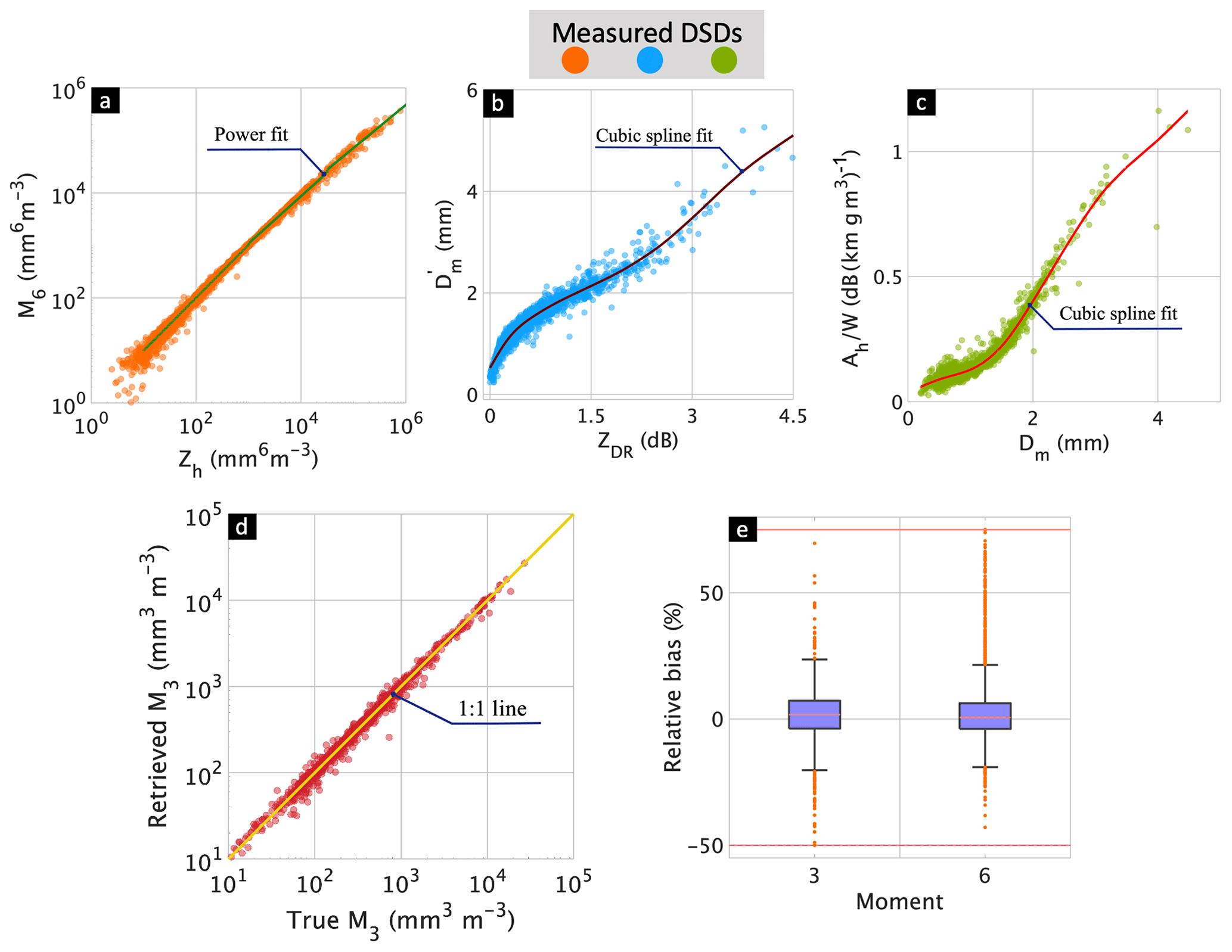
Figure 8 (a) Retrieval of M₆ as a power law of Z_h as per Eq. (2); each data point is based on a 3 min averaged complete spectrum from either the Greeley, CO, or Huntsville, AL, site. The simulations of X-band Z_h, Z_DR, and A_h are based on assumptions in Sect. 3.3. (b) Retrieval of $D_{\mathrm{m}}^{\prime }$ from Z_DR along with smoothed cubic spline fit. (c) Same but for retrieval of A_h∕W from D_m, where W is the rain water content. (d) The retrieved M₃ versus “true” M₃. (e) Box plots of RB for retrieval of M₃ and M₆ (which is a measure of the deviation of the fitted values from the “true” values because of DSD variability). The inter-quartile range is given by the “height” of the dark blue box, while the orange horizontal line inside the blue box is the median. The outliers are shown as orange circles; <10 % are estimated to be outliers. The orange horizontal lines on top and bottom indicate the upper and lower outer fences, respectively.

The next step is to retrieve A_h∕W from D_m (adapted from Jameson, 1993, who used a third-order polynomial fit) for which we employ a smoothed spline fit. Here A_h is in dB km⁻¹ and W is the rain water content in gm⁻³. We restricted the range of A_h∕W at X-band to between 0.02 and 2 to avoid outliers. The smoothing spline fit is shown in Fig. 8c, which again provides a visibly good fit and is robust if the D_m falls outside the specified range. The retrieval of M₃ follows from

$$\begin{array}{}\text{(3)}& {\displaystyle }{M}_{\mathrm{3}}={\displaystyle \frac{\mathrm{6000}}{\mathit{\pi }}}W={\displaystyle \frac{\mathrm{6000}}{\mathit{\pi }}}{\displaystyle \frac{A_{\mathrm{h}}}{f\left(D_{\mathrm{m}}\right)}},\end{array}$$

where f(D_m) is the spline fit shown in Fig. 8c. The scatter plot of retrieved M₃ versus “true” M₃ is shown in Fig. 8d. This multi-step procedure was devised to minimize the parameterization (or algorithm) errors, but we note it is by no means the only way to achieve this.

It is known that the absorption cross section (specifically for X-band used here) depends on the temperature T via the 𝕀m{ε_r}, where ε_r is the dielectric constant of water. For a given W, the integral of the extinction cross section weighted by N(D) or A_h increases with colder water temperature but also depends on D_m (Jameson, 1993). Scattering simulations were performed for 8 and 20 ^∘C and the spline fits of A_h∕W versus D_m were compared. For low values of D_m, the maximum difference was 35 %, occurring at D_m=0.75 mm (with A_h∕W larger at 8^∘ relative to 20 ^∘C as expected), but a crossover occurs near D_m=1.8 mm and the deviations increase in the opposite direction, with a maximum deviation of −15 % at D_m=3 mm (A_h∕W at 20 ^∘C larger than at 8 ^∘C due to scattering loss). Recall that the National Weather Service (NWS) sounding at Denver about 65 km away showed a surface T of 12 ^∘C. A lower temperature of 8 ^∘C was used in the scattering calculations to approximately account for cooling of the atmosphere near Easton due to rainfall. The other temperature dependence is the coefficient α in the relation A_h=αK_dp used in the iterative ZPHI method. This method involves finding an optimized α for each beam and is assumed to account for temperature changes. Since the actual drop temperature is not known and the surface T of 12 ^∘C is close to the assumed T of 8 ^∘C, the spline fit shown in Fig. 8c is considered to be sufficiently accurate for the retrieval of M₃. We note that Diederich et al. (2015) found that the R(A_h) relation at X-band had a relatively “weak” dependence on temperature. Their fitted power law was $\mathrm{45.5}{A}_{\mathrm{h}}^{\mathrm{0.83}}$ at 10 ^∘C to $\mathrm{43.5}{A}_{\mathrm{h}}^{\mathrm{0.79}}$ at 20 ^∘C. At R=10 mm h⁻¹, the A_h at 10 ^∘C is larger than at 20 ^∘C by 6.8 %, while, at 100 mm h⁻¹, the A_h at 10 ^∘C is lower than at 20 ^∘C by −10.8 %; this crossover is consistent with our calculations above.

The evaluation of the algorithm error is done by defining the absolute bias of retrieved M, where M=M₃ or M₆, as Δ=(M(retrieved)–M(“true”)) and the relative bias $\mathrm{RB}=\mathrm{100}\times \mathrm{\Delta }/M$(“true”) as a percentage. To show the range of the RB and the distribution features (such as the median and 25th and 75th percentiles) in compact form, box plots for M₃ and M₆ are shown in Fig. 8e. The $\mathit{\{}\mathrm{25}\text{th},\text{median},\mathrm{75}\text{th}\mathit{\}}$ percentile values for M₃ and M₆ are $\mathit{\{}-\mathrm{3.8},\mathrm{1.7},\mathrm{7.2}\mathit{\}}$ and $\mathit{\{}-\mathrm{3.8},\mathrm{0.63},\mathrm{6.2}\mathit{\}}$, respectively. Note that the median relative bias is close to 0 and lies at the center of the box showing very low skewness. The interquartile range (IQR) is nearly the same for both M₃ and M₆. The extremities of the blue boxes are called hinges which span the IQR or the first (lower hinge) and third (upper hinge) quartiles. The orange line within the blue boxes indicates the median. The outliers (orange circles) lie beyond the first and third quartiles by at least 1.5 times the IQR. In particular, 1.5 and 3 times the IQR limit above (below) the upper (lower) hinge of a box are called the upper (lower) inner fence and upper (lower) outer fence, respectively (Theus and Urbanek, 2008). A point beyond an inner fence on either side is considered a mild outlier, while a point beyond an outer fence is an extreme outlier. The largest value below the upper inner fence and the smallest value above the lower inner fence are indicated by shorter grey horizontal lines called whiskers, within which lie extreme values that are not considered outliers. If there are no points beyond a whisker, corresponding inner and outer fences are not plotted. Similarly, if there are no samples between the inner and outer fences, only the inner fence is shown in the plot. Otherwise, the inner fence is generally omitted, and only the outer fence is depicted. For example, Fig. 8e shows only outer fence lines on top and bottom. While plotting multiple box plots in the same figure, only a common fence line that is closest and outside of all boxes is shown. The number of outliers for M₃ is only 6.5 % of the total number of samples, while for M₆ it is 9.5 %. It is interesting to note that the mean RBs for M₃ and M₆ are, respectively, −1.1 % and 0 %, which are close to the median values, meaning that there is low skewness in the relative error distributions.

Histograms of Δ∕〈M〉 showed Gaussian-like shapes (not shown here). The variances of Δ normalized by 〈M〉² were 0.106 and 0.606 for M=M₃ and M=M₆, respectively; the corresponding fractional standard errors (FSEs) were, respectively, 0.32 and 0.778. These variances are referred to as variances due to parameterization or retrieval algorithm errors which can be added to the variances of the corresponding radar measurement errors to arrive at the total error variances. It is demonstrated (in the Appendix) that the retrieval algorithm error for M₆ dominates the total error variance, whereas for M₃ the retrieval algorithm and radar measurement errors are comparable.

5 Validation of radar-retrieved moments

The validation procedure essentially follows methods already developed for comparing radar-retrieved rain rates with disdrometers or gages (e.g., Bringi et al., 2011b). The mean Lee-filtered Z_h, Z_dr, and A_h time-series data (see Fig. 6) were used to retrieve time series of {M₃,M₆}. Using Eq. (1) with the climatological $h_{\text{GG}}(x;\mathit{\mu },c)$ shown in Fig. 7, the other moments (0 through 2, 4 through 5, and 7) were computed. Retrievals and performance statistics were calculated for 20:00–21:30 UTC. The period after 21:30 UTC was omitted from this analysis because of the heavy rain observed on radome during the last half-hour of the event.

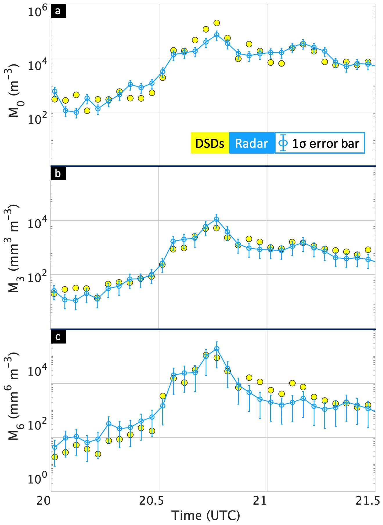
Figure 9 Time series of radar-derived moments and from complete DSDs over the disdrometer site. The radar estimates are mean ±1σ error bars. (a) Moment M₀; (b)–(c) same but for M₃ and M₆.

Figure 9 shows the time series of radar-retrieved M₀, M₃, and M₆ with those calculated from the 3 min complete DSDs. The radar retrievals in Fig. 9 show the mean with ±1σ error bars, where σ is the standard deviation. The mean value at each time step is obtained from the Lee-filtered values of $\mathit{\{}{Z}_{\mathrm{h}},Z_{\mathrm{dr}},A_{\mathrm{h}}\mathit{\}}$ which are used to retrieve the {M₃,M₆}. Then, using Eq. (1), the radar retrievals of M₀ and other moments are obtained. The error bars or the variances consist of the sum of two terms, namely the parameterization error variances (described above) and the radar measurement errors which are uncorrelated. The Appendix describes the procedure to estimate the total error variances for moments such as M₀ and the other non-reference moments in terms of the total error variances of M₃ and M₆. The last column in Table A1 gives the normalized total error variances for each moment. In Fig. 9, the standard deviation is obtained at each time step by taking the square root of the normalized variances (or the FSE) from the last column of Table A1 for M₀, M₃, and M₆, with respective FSE values being $\mathit{\{}\mathrm{0.385},\mathrm{0.535},\mathrm{0.805}\mathit{\}}$. The σ at each time step in Fig. 9 is calculated by multiplying the radar-retrieved M₀, M₃, and M₆ at each time step by the corresponding FSE.

Figure 9a illustrates the intercomparison of M₀ which is the most difficult to estimate using moments {M₃,M₆} (see Morrison et al., 2019, RBa, and Raupach et al., 2019). The error bars on the radar estimates are the total errors with FSE = 0.385; see Appendix. The agreement with “ground truth” is visually quite remarkable considering that other error sources such as attenuation correction or point-to-area variance have been neglected (Ciach and Krajewski, 1999; Bringi et al., 2011b). The total concentration (M₀) in this event ranges from 100 per m³ to 100 000 per m³ at the time of peak rainfall over Easton at 20:45 UTC. Figures 9b and c show time series of M₃ and M₆, respectively. The M₃ retrievals are in excellent agreement with “ground truth” (total FSE = 0.535 with 63 % of the variance due to measurement error and 37 % due to algorithm error). Figure 9c compares M₆, and now the agreement degrades slightly. But the error bars have also increased substantially (total FSE = 0.805 with nearly 93 % of the variance due to algorithm errors). The M₆ varies from 10 to 10⁵ mm⁶ m⁻³ (or equivalently 10 to 50 dBZ), the peak value at 20:45 UTC being in excess of 50 dBZ. Note that M₀ and M₃ are the moments prognosed by “bulk” double-moment numerical schemes (actually M₀ and mass mixing ratio). So, radar retrievals could potentially play a role in evaluating the microphysical parameterizations in such models (e.g., Meyers et al., 1997).

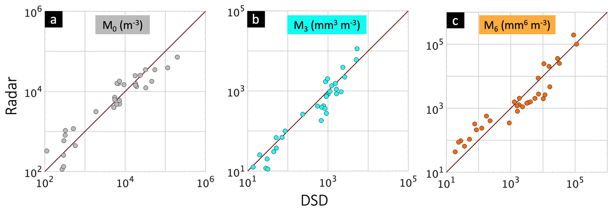
Figure 10 Scatter plot of radar-derived moments versus “true” moments from the complete DSD data on log ₁₀ scales. (a) M₀, (b) M₃, and (c) M₆.

Table 2 Statistics of the RB (median and IQR range). The correlations are between radar-retrieved moments and directly computed moments from the complete DSD measured by disdrometers.

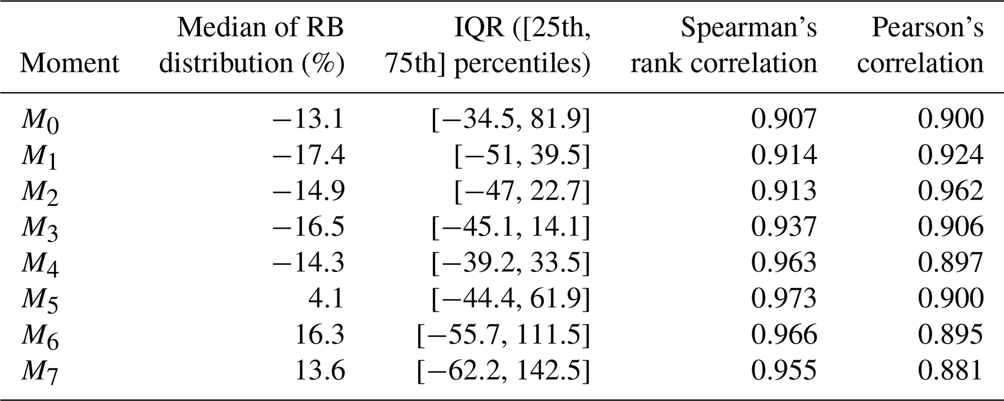
The scatter plots of M₀, M₃, and M₆ are shown in Fig. 10. The high correlation is quite striking and substantiated by both Pearson's and Spearman's rank correlation values in Table 2. Note that Spearman's measures only the monotonic relationship between the correlated variables, while Pearson's provides a measure of both monotonicity and linearity. The RB (%) was defined in Sect. 4.2; for each moment (M₀ through M₇) the corresponding box plots are shown in Fig. 11. We note that there are very few or no outliers for most of the moments. Table 2 gives the median (%) and the IQR range. The IQR range is smallest for M₃. This is expected because it is one of the reference moments. The median of the RB is “best” for M₅, with a symmetric IQR range indicating very low skewness. The median RBs for moments M₀ through M₄ are around −15 %, but the skewness is significant for M₀ and progressively less for M₁ through M₅. It might be unexpected that the retrieval of M₆ being one of the reference moments is less accurate than M₅. One possible reason is that, at X-band, the larger drops are resonant-sized and the Z_H does not vary as M₆ but is rather closer to M₅ depending on the drop sizes. Figure 7a, in fact, shows that the fit for M₆ has a smaller slope for Z_H>37 dBZ because of resonant scattering. The median RB for M₆ and M₇ are <17 %, but the IQR indicates positive skewness (i.e., radar estimates are larger than “truth”).

The difficulty in retrieving M₀ from higher-order moments {M₃,M₆} is clear from the box plot but nevertheless viable with relatively low median values and high correlation coefficients. However, the accuracy of all moment-order retrievals, and especially the lower order, strongly depends on the climatological shape of h(x) for x<0.75 reflecting the shape of the small drop end (concave up for negative μ). This is irrespective of well-constrained measurement and parameterization errors in the retrieval of the reference moments {M₃,M₆}.

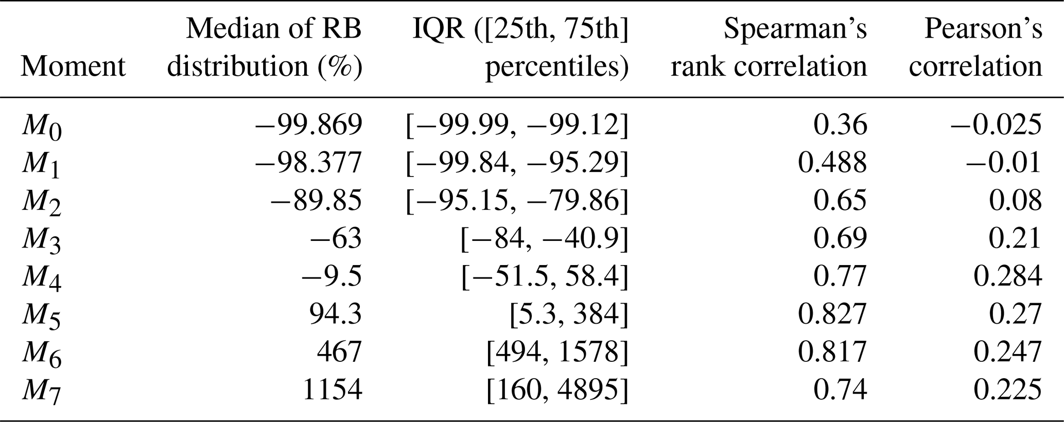
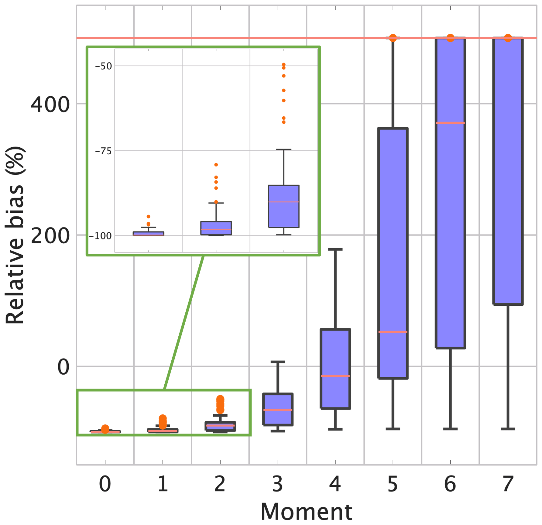
To illustrate this further, the “incomplete” spectra from 2DVD data alone, which are known to underestimate the numbers of small drops, are used to establish the “climatological” h(x) for which the fitted G-G shape parameters are μ=0.54 and c=3.07 (see Fig. 7). The radar moment retrieval steps are the same as before except for the now different h(x). The “true” moments are the same as before, being based solely on the complete DSD spectra. The new box plots of RB are shown in Fig. 12. Note that now the lower-order moments (M₀ through M₂) are severely underestimated, with median RB slightly less than −100 %, but the IQR is highly compressed, reflecting a distribution of RB which is concentrated as a delta function. The median RB for moments M₆ and M₇ is very large, >400 % with large IQR. Moments M₃ through M₅ show more “normal” RB distributions with median values of RB in the range −60 % to 90 %, the minimum occurring for M₄. However, Pearson's correlation coefficients, as shown in Table 3, are very low for all moments, implying (practically) no linear variation between the moments. Spearman's rank correlation is higher for moments M₄ through M₇, implying that a nonlinear monotonic relationship between moments probably exists. The results in Table 3 vis-à-vis Table 2 demonstrate the importance of determining the “climatological” h(x) using the complete DSDs for accurate radar-based retrievals of the lower-order moments. In Table 3, the floor for RB is $>-\mathrm{1}$.

Table 3 As in Table 2 except h(x) is from incomplete 2DVD DSDs only.

Finally, the radar retrievals are examined from the perspective of identifying coherent “time tracks” as the main echo traversed the Easton site. To this end, Fig. 13 shows tracks in (a) the D_m–M₀ plane, (b) the D_m–W plane, and (c) the $D_{\mathrm{m}}^{\prime }$–M₆ plane from 20:12 to 21:12 UTC. Note that we use $D_{\mathrm{m}}^{\prime }$ in panel (c) because it is more closely related to Z_dr. For example, panel (a) shows the initial rapid rise in D_m from 1.5 to 2.2 mm (data point numbers 3 to 8 or approximately 2030–2045) with a corresponding increase in M₀ (total number concentration) from 1000 to nearly 100 000 per m³. Together with similar behavior in panel (b) where W increases from ≤2 to 6 g m⁻³ and in (c) where M₆ increases from 30 to >50 dB, this suggests the strong echo aloft descending to the surface over Easton. This inference was based on examining successive volume scans from KFTG (WSR-88D in Denver, CO, located about 60 km away) and noting the descent of the echo aloft to the surface at 20:45 UTC. After the peak, the track (data points 8 to 11 or 20:45 to 20:57 UTC) reflects a rapid decrease in M₀ and D_m and from panel (b) a rapid decrease in W with a corresponding rapid decrease in M₆, reflecting advection of the rain shaft to the north of Easton. Towards the end (last five data points from 20:57 to 21:12 UTC) the D_m decrease is slowed down (from 1.5 to 1 mm), while the M₀ increases modestly from 10 000 to 15 000 per m³. This compensatory effect results in the rain water content being more or less steady (at 0.5 g m⁻³), while M₆ decreases from 37 to 33 dB (panels b and c, last five data points). The echo structure during this latter time period was transitioning from earlier descent of the strong echo over Easton to more of a steady rain event.

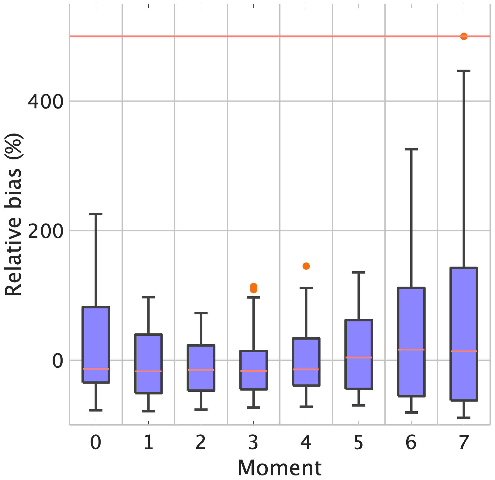
Figure 11 Box plots of relative bias (RB) as in Fig. 8e except between radar-derived moments and completed DSD moments (“truth”). The orange horizontal line on top indicates the upper inner fence.

Figure 12 As in Fig. 11 except that the incomplete 2DVD DSDs are used to determine h(x) (see dashed line in Fig. 7). Inset shows magnified box plots for M₀ through M₂. The orange horizontal line on top indicates the upper inner fence.

6 Discussion

The polarimetric radar retrieval and validation of the lower-order moments of the DSD have not received much attention in the past, except for RBb. However, substantial literature exists in using either the un-normalized gamma model of Ulbrich (1983) or the normalized gamma model of Testud et al. (2001) to estimate the three parameters $\mathit{\{}{N}_{\mathrm{0}},\mathit{\mu },\mathrm{\Lambda }\mathit{\}}$ or $\mathit{\{}{N}_{\mathrm{w}},\mathit{\mu },D_{\mathrm{m}}\mathit{\}}$. As shown by L04, the Testud et al. (2001) formulation falls into double-moment normalization with reference moments M₃ and M₄, with h(x) being a special case of the G-G with c=1; hence, there is only one shape parameter μ. Note that $\mathit{\mu }={\mathit{\mu }}_{\text{ULB}}+\mathrm{1}$, where μ_ULB is the shape parameter defined in Ulbrich (1983).

Many studies have attempted to retrieve the three parameters $\mathit{\{}{N}_{\mathrm{w}},\mathit{\mu },D_{\mathrm{m}}\mathit{\}}$ using polarimetric measurements $\mathit{\{}{Z}_{\mathrm{h}},Z_{\mathrm{dr}},K_{\mathrm{dp}}\mathit{\}}$ at S-, C-, and X-bands, but they are too numerous to discuss herein (e.g., Bringi et al., 2003; Brandes et al., 2003; Park et al., 2005b; Gorgucci et al., 2008; Anagnostou et al., 2013, to mention a few). Anagnostou et al. (2013) compared three different methods of retrieving N_w but found that validation was very difficult, commenting that “… the estimation of N_w by all algorithms is significantly affected by noise or other factors like radar volume versus point (disdrometer) measurement-scale mismatch and spatial separation.”

However, neither N₀ nor N_w is the same as M₀, which is simply the total number concentration that scales the gamma pdf. The estimation of either N₀ (or N_w) depends on the shape parameter (or the slope parameter Λ). Typically, the μ is assumed to be fixed or empirically derived as f(Λ) or another function of D_m (Schinagl et al., 2019). Of course, any moment of the gamma pdf can be derived as functions of the three parameters in the gamma model, but very few validations of, for example, M₀ have been conducted. Brandes et al. (2003) used an empirically derived μ–Λ relation based on 2DVD data. Using Z_h and Z_dr radar measurements at S-band, they retrieved N₀ and Λ and obtained the M₀ as $N_{\mathrm{0}}{\mathrm{\Lambda }}^{-(\mathit{\mu }+\mathrm{1})}$. They analyzed one convective event (with Z_H varying from 10 to 55 dBZ) and showed the mean of log ₁₀(M₀) from radar was 2.74 compared with 2.84 from 2DVD measurements (or 550 and 690 per m³, which are much smaller than the values obtained here; see Fig. 10a). The key point is that the mean μ was in the range 3–4, which is caused by truncation at the small drop end of the DSD.

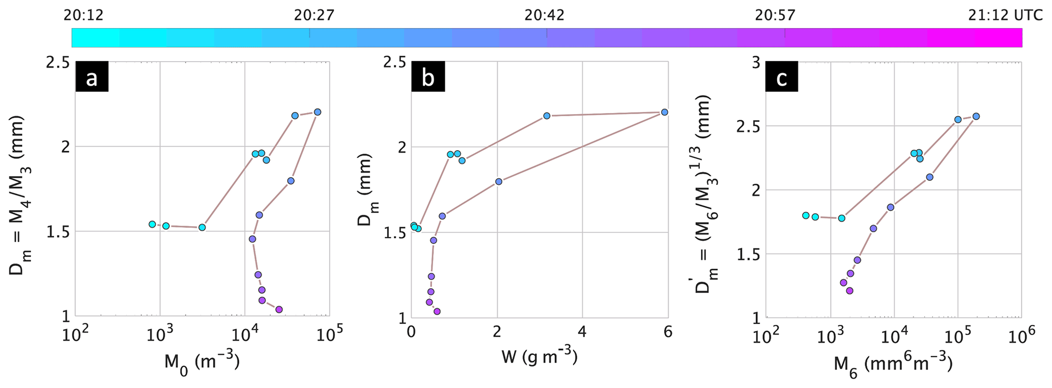
Figure 13 Time tracks of radar-derived variables in the (a) D_m versus M₀ plane showing the trajectories as a function of time (color coded) over approximately an hour. Each data point reflects the radar-retrieved moments (M₀) or ratio of moments (M₄∕M₃) (see Fig. 9). (b)–(c) Same but time tracks in the D_m versus W plane and $D_{\mathrm{m}}^{\prime }$ versus M₆ planes, respectively. Again, all quantities are from radar-retrieved moments.

Wen et al. (2018) describe a different method of estimating the DSD parameters of the gamma distribution and the lower-order moments based on an inverse model where the input is $\mathit{\{}{Z}_{\mathrm{dr}},K_{\mathrm{dp}}/Z_{\mathrm{h}}\mathit{\}}$ and the output is {μ,D_max}, where D_max is the maximum diameter of the retrieved gamma DSD. Their approach follows the well-known k-nearest-neighbor (k-NN) classification from the pattern recognition literature (Shakhnarovich et al., 2006). This algorithm stores all input–output associations from the available data as a “training” set. When a new $\mathit{\{}{Z}_{\mathrm{dr}},K_{\mathrm{dp}}/Z_{\mathrm{h}}\mathit{\}}$ input is presented, the algorithm assigns it the {μ,D_max} output class that is the most common amongst the k nearest (training set) neighbors of the new input. The k-NN is particularly suitable when large training data are available. Wen et al. (2018) used Euclidean distance to define the closeness of neighbors, although other distance functions are also employed in k-NN algorithms. They applied an empirical μ–Λ relation based on 2DVD data, while N₀ is obtained a posteriori using Z_h, μ, Λ, and D_max. Their training set comprising Z_dr and K_dp∕Z_h was generated using a polynomial function whose inputs μ and D_max are drawn from 10-year disdrometer data with constraints $\mathit{\mu }\in [\mathrm{-}\mathrm{3},\mathrm{20}]$, $D_{\text{max}}\in [\mathrm{1.7}\text{mm},\mathrm{8}\text{mm}]$, and D_max>D_m. The test stage used S-band radar data from a WSR-88D unit (KTLX) located in Oklahoma City, OK. A large database was analyzed, and the moments M₀, M₂, M₄, and M₆ were computed from $\mathit{\{}{N}_{\mathrm{0}},\mathit{\mu },\mathrm{\Lambda },D_{\text{max}}\mathit{\}}$. The validation results in terms of what they define as relative absolute error (RAE) ranged from 0.986 (or 98.6 %) for M₀ to 0.455 (or 45.5 %) for M₆, while Pearson's correlation coefficient between radar-based M₀ and 2DVD M₀ “truth” was 0.651 (the maximum correlation coefficient for other moments was <0.7). The predictive performance of k-NN was quantified through root relative squared error (RRSE), which computes the difference between the k-NN-predicted values with the actual ones relative to when a simple predictor is used. More than characterizing the accuracy of computation of moments, both RAE and RRSE give an indication of the efficacy of k-NN-based prediction over the most basic mean-value prediction method. Wen et al. (2018) reported low RRSE for M₂, M₄, and M₆, whereas it was large (>1) for M₀. They commented that “the inverse model […] produced DSD retrievals with large uncertainties due to the measurement errors, noise, and sampling problems of the instruments.”

The RBb article used X-band radar Z_h to retrieve M₆ and {Z_dr,K_dp} to retrieve M₃. Our approach is similar except that we use A_h instead of K_dp. There are several advantages to using A_h (similar to its use in estimating R at X-band; Diederich et al., 2015). For instance, A_h is always positive, is highly correlated with Z_h variations, thus preserving the spatial resolution, and, at X-band, has decent dynamic range. The article used several networks of the Parsivel disdrometer from three locations to derive h(x) and the G-G fit, but their fit was more similar to that shown in Fig. 7 (black dashed line); in fact, they obtained a larger μ (2.22) and smaller c (1.69). The higher value of μ gives a more convex down shape at small x (relative to black dashed line in Fig. 7), while smaller c results in slower fall of the tail of the distribution. The other issue they had to deal with was the “noisy” Z_dr and K_dp measurements when Z_H<37 dBZ. They “restored” the noisy Z_dr by estimating it using a power law with Z_h, while noisy K_dp was restored using power laws of Z_h and Z_dr. They also commented that the majority of radar-measured Z_H was <37 dBZ. So, noise correction dominated the statistics of their moment retrievals. Their radar retrievals of moments were based on a large dataset from three regions (two in Europe and one in Iowa, US). While they obtained median values of RB in the range 4 % to −46 %, their r² (squared Pearson's correlation) coefficient between radar moments and ground “truth” was very low (0.05 to 0.33), similar to what we obtained in Table 3. They ascribed their poor correlation to spatial representativeness errors, height of the radar pixels above the Parsivel network at longer ranges, and other factors, similarly to Anagnostou et al. (2013).

7 Summary

We demonstrated a proof-of-concept of the viability of radar retrieval of lower-order moments of the DSD using specific attenuation A_h in addition to Z_h and Z_dr at X-band (an extension of RBb) via a case study approach. The use of specific attenuation (from the iterative ZPHI method) is consistent with its many advantages for rain rate estimation. The multi-cell convective complex which occurred in the area near Greeley, CO, on 23 May 2015 was a target of opportunity as the CSU-CHILL radar system was available to scan the echo complex with a single elevation angle PPI every 90 s over a period of around 90 min. The instrumented site at Easton located 13 km to the south of the radar had an MPS and 2DVD sited inside a DFIR wind shield which made it possible to acquire the “complete” drop spectra with high resolution (50 µm) for the small drop end and good resolution (about 170 µm) for drops ≥0.7 mm. The moment retrieval was based on the double-moment scaling/normalization framework of Lee et al. (2004). Two reference moments {M₃,M₆} along with a “climatological” estimate of the underlying shape of the scaled/normalized DSDs fitted to the G-G distribution formed the basis of the method. The {M₃,M₆} retrieval algorithms were trained using scattering simulations of Z_h, Z_dr, and A_h using 2928 3 min averaged DSDs from Greeley, CO, and Huntsville, AL. The parameterization (or algorithm) errors due to DSD variability about the smoothed spline fits were computed.

Polarimetric X-band radar data (acquired with an exceptionally narrow 3 dB beamwidth of 0.33^∘) were extracted from a small polar box surrounding the instrumented site, and moments M₀ through M₇ were estimated and validated against ground “truth” from the moments of the complete spectra using MPS and 2DVD. Using a variety of validation measures such as box plots of RB, time-series comparisons, scatter plots, and correlation coefficients, it was determined that good accuracy was obtained for the radar-based moments well beyond what has been possible hitherto. For moments M₀ through M₂, the RB was <15 % in magnitude, with Pearson's correlation coefficients between radar-derived moments and DSD-based moments exceeding 0.9. A detailed analysis of radar fluctuations or measurement errors propagating to the variance of the moment estimates was performed; in addition, the total variance due to both parameterization and measurement errors was tabulated.

The coherency of “time track” plots of radar-retrieved quantities in the D_m versus M₀, D_m versus W, and $D_{\mathrm{m}}^{\prime }$ versus M₆ planes as the main 55 dBZ echo passed over the site (as well as 20 min prior to and 20 min after this passage) demonstrated the potential use for precipitation evolution studies for this DSD-retrieval technique. One caveat is that a much larger database is needed before concrete conclusions are drawn. In particular, the possibility of the very narrow beam of 0.33^∘ and the close range (13 km) to the instrumented site contributing to very good validation statistics, found herein relative to other studies, requires investigations with more data.

Appendix A

The error model (Bringi and Chandrasekar, 2001) we adopt here is an additive one, $\widehat{X}=X+{\mathit{\epsilon }}_{\mathrm{m}}+{\mathit{\epsilon }}_{\mathrm{p}}$, where $\widehat{X}$ is the estimated (or retrieved) quantity, X is the “true” value, and ε_m and ε_p are, respectively, the radar measurement and parameterization (or algorithm) errors. The ε_m and ε_p are zero mean, uncorrelated errors so that $\mathbb{E}\mathit{\left\{}\widehat{X}\mathit{\right\}}=X$. Thus, it follows that $\mathrm{Var}(\widehat{X}-X)=\mathrm{Var}\left({\mathit{\epsilon }}_{\mathrm{m}}\right)+\mathrm{Var}\left({\mathit{\epsilon }}_{\mathrm{p}}\right)$. For different rain rate estimators such as R(Z_h), R(Z_h,Z_dr), and R(K_dp), the $\mathrm{Var}\left(\widehat{R}\right)/{\stackrel{\mathrm{‾}}{R}}^{\mathrm{2}}$ is expressed in terms of the standard deviations of Z_h, Z_dr, and K_dp which are 1 dBZ, 0.3 dB, and 0.3^∘ km⁻¹, respectively (Thurai et al., 2017b).

Errors due to attenuation correction are not considered because most of the attenuation occurred at ranges beyond the instrumented site (see Fig. 5). We refer to Thurai et al. (2017b) for evaluation of such errors.

A1 Radar measurement errors

We consider error variances of the retrieval of M₆ and M₃ first and then the other moments. Since M₆ is retrieved as a power law of $Z_{\mathrm{h}}^{\mathrm{0.8}}$ (the exponent is approximate),

$$\begin{array}{}\text{(A1)}& {\displaystyle \frac{\mathrm{Var}\left(M_{\mathrm{6}}\right)}{{\stackrel{\mathrm{‾}}{M_{\mathrm{6}}}}^{\mathrm{2}}}}={\mathrm{0.8}}^{\mathrm{2}}{\displaystyle \frac{\mathrm{Var}\left(Z_{\mathrm{h}}\right)}{{\stackrel{\mathrm{‾}}{Z_{\mathrm{h}}}}^{\mathrm{2}}}},\end{array}$$

where Z_h has units of mm⁶ m⁻³. Assuming the standard deviation of the radar measurement error is typically 1 dB, we get $\mathrm{Var}\left(Z_{\mathrm{h}}\right)/{\stackrel{\mathrm{‾}}{Z_{\mathrm{h}}}}^{\mathrm{2}}=\mathrm{0.067}$. This implies that

$$\begin{array}{}\text{(A2)}& {\displaystyle }\mathrm{Var}\left(M_{\mathrm{6}}/{\stackrel{\mathrm{‾}}{M_{\mathrm{6}}}}^{\mathrm{2}}\right)=\mathrm{0.043}.\end{array}$$

The variance of M₃ is more complicated because it is a multi-step procedure as described in Sect. 4 involving smoothed spline fits. We use approximate power-law fits for estimating Var(M₃) as follows. We have

$$\begin{array}{}\text{(A3)}& {\displaystyle }{D}_{\mathrm{m}}^{\prime }\approx \mathrm{1.18}(Z_{\mathrm{dr}}{)}^{\mathrm{1.5}},\end{array}$$

and

$$\begin{array}{}\text{(A4)}& {\displaystyle \frac{A_{\mathrm{h}}}{W}}\approx \mathrm{0.09}{D}_{\mathrm{m}}^{\mathrm{2}},\text{for}{D}_{\mathrm{m}}>\mathrm{1}\text{mm}.\end{array}$$

Thus,

$$\begin{array}{}\text{(A5)}& {\displaystyle \frac{\mathrm{Var}\left(M_{\mathrm{3}}\right)}{{\stackrel{\mathrm{‾}}{M_{\mathrm{3}}}}^{\mathrm{2}}}}={\displaystyle \frac{\mathrm{Var}\left(A_{\mathrm{h}}\right)}{{\stackrel{\mathrm{‾}}{A_{\mathrm{h}}}}^{\mathrm{2}}}}+{\displaystyle \frac{\mathrm{4}\mathrm{Var}\left(D_{\mathrm{m}}\right)}{{\stackrel{\mathrm{‾}}{D_{\mathrm{m}}}}^{\mathrm{2}}}}.\end{array}$$

Since D_m is linear with $D_{\mathrm{m}}^{\prime }$, and assuming the standard deviation of the radar measurement of Z_DR is 0.3 dB,

$$\begin{array}{}\text{(A6)}& {\displaystyle \frac{\mathrm{Var}\left(M_{\mathrm{3}}\right)}{{\stackrel{\mathrm{‾}}{M_{\mathrm{3}}}}^{\mathrm{2}}}}={\displaystyle \frac{\mathrm{Var}\left(A_{\mathrm{h}}\right)}{{\stackrel{\mathrm{‾}}{A_{\mathrm{h}}}}^{\mathrm{2}}}}+{\displaystyle \frac{\mathrm{9}\mathrm{Var}\left(Z_{\mathrm{dr}}\right)}{{\stackrel{\mathrm{‾}}{Z_{\mathrm{dr}}}}^{\mathrm{2}}}},\end{array}$$

where Z_dr is a ratio and $\mathrm{Var}\left(Z_{\mathrm{dr}}\right)/{\stackrel{\mathrm{‾}}{Z_{\mathrm{dr}}}}^{\mathrm{2}}=\mathrm{0.0051}$:

$$\begin{array}{}\text{(A7)}& {\displaystyle \frac{\mathrm{Var}\left(M_{\mathrm{3}}\right)}{{\stackrel{\mathrm{‾}}{M_{\mathrm{3}}}}^{\mathrm{2}}}}={\displaystyle \frac{\mathrm{Var}\left(A_{\mathrm{h}}\right)}{{\stackrel{\mathrm{‾}}{A_{\mathrm{h}}}}^{\mathrm{2}}}}+\mathrm{0.0046}.\end{array}$$

From Thurai et al. (2017b, Appendix, A5),

$$\begin{array}{}\text{(A8)}& {\displaystyle \frac{\mathrm{Var}\left(A_{\mathrm{h}}\right)}{{\stackrel{\mathrm{‾}}{A_{\mathrm{h}}}}^{\mathrm{2}}}}={\mathrm{0.8}}^{\mathrm{2}}{\displaystyle \frac{\mathrm{Var}\left(Z_{\mathrm{h}}\right)}{{\stackrel{\mathrm{‾}}{Z_{\mathrm{h}}}}^{\mathrm{2}}}}+{\displaystyle \frac{\mathrm{Var}\left(K_{\mathrm{dp}}\right)}{{\stackrel{\mathrm{‾}}{K_{\mathrm{dp}}}}^{\mathrm{2}}}},\end{array}$$

assuming that A_h varies as $Z_{\mathrm{h}}^{\mathrm{0.8}}$ used in the ZPHI method. The standard deviation of the K_dp measurement is typically 0.3^∘ km⁻¹ and that of Z_H is 1 dB. Further, the mean K_dp for our data ≈1^∘ km⁻¹ (Fig. 6c) but is variable in time. In any case,

$$\begin{array}{}\text{(A9)}& {\displaystyle \frac{\mathrm{Var}\left(A_{\mathrm{h}}\right)}{{\stackrel{\mathrm{‾}}{A_{\mathrm{h}}}}^{\mathrm{2}}}}\approx \left(\mathrm{0.64}\right)\left(\mathrm{0.067}\right)+\mathrm{0.09}=\mathrm{0.133}.\end{array}$$

Substituting above in Eq. (A6) yields

$$\begin{array}{}\text{(A10)}& {\displaystyle \frac{\mathrm{Var}\left(M_{\mathrm{3}}\right)}{{\stackrel{\mathrm{‾}}{M_{\mathrm{3}}}}^{\mathrm{2}}}}=\mathrm{0.133}+\mathrm{0.046}=\mathrm{0.18}.\end{array}$$

A2 Variances of the other moments

From Lee et al. (2004), the other moments M_k can be expressed as power laws of the reference moments M₃ and M₆. They are of the form $M_k=C_k{M}_{\mathrm{3}}^{p_k}{M}_{\mathrm{6}}^{-q_k}$, where p_k and q_k are rational numbers and C_k is some constant. The variance of M_k needs more elaboration as X≡M₃ and Y≡M₆ are correlated. This correlation arises because A_h is a power law with Z_h, i.e., $Z_{\mathrm{h}}^{\mathrm{0.8}}$ in the ZPHI method. Together with M₆ being a power law with Z_h, the M₃ and M₆ are correlated with a correlation coefficient of 0.93 obtained from radar-derived M₃ and M₆. For the kth moment M_k, $p_k=\frac{\mathrm{6}-k}{\mathrm{3}}$ and $q_k=\frac{\mathrm{3}-k}{\mathrm{3}}$ for $k=\mathrm{0},\mathrm{1},\mathrm{\cdots },\mathrm{7}$, $k\ne \mathrm{3},\mathrm{6}$. The objective is to derive $\frac{\mathrm{Var}\left(M_k\right)}{{\stackrel{\mathrm{‾}}{M_k}}^{\mathrm{2}}}$ in terms of $\frac{\mathrm{Var}\left(M_{\mathrm{3}}\right)}{{\stackrel{\mathrm{‾}}{M_{\mathrm{3}}}}^{\mathrm{2}}}$, $\frac{\mathrm{Var}\left(M_{\mathrm{6}}\right)}{{\stackrel{\mathrm{‾}}{M_{\mathrm{6}}}}^{\mathrm{2}}}$, and Cov(M₃,M₆).

In the sequel, for notational simplicity, we drop the subscripts k. Then, for certain rational numbers p and q, any moment M is a function of these two random variables as

$$\begin{array}{}\text{(A11)}& {\displaystyle }M\mathit{\triangleq }f\left(M_{\mathrm{3}},M_{\mathrm{6}}\right)=C{\displaystyle \frac{M_{\mathrm{3}}^p}{M_{\mathrm{6}}^q}}=C{\displaystyle \frac{X^p}{Y^q}}.\end{array}$$

Consider the parameter vector $\mathit{\theta }=(\stackrel{\mathrm{‾}}{X},\stackrel{\mathrm{‾}}{Y})$. Then, second-order Taylor series approximation of f(X,Y) around θ produces

$$\begin{array}{}\text{(A12)}& \begin{array}{rl}M& \approx f\left(\mathit{\theta }\right)+f_x^{\prime }\left(\mathit{\theta }\right)(X-\stackrel{\mathrm{‾}}{X})+f_y^{\prime }\left(\mathit{\theta }\right)(Y-\stackrel{\mathrm{‾}}{Y})\\ & +{\displaystyle \frac{\mathrm{1}}{\mathrm{2}}}\left\{f_{xx}\prime \prime \prime \left(\mathit{\theta }\right)(X-\stackrel{\mathrm{‾}}{X}{)}^{\mathrm{2}}+\mathrm{2}{f}_{xy}\prime \prime (\mathit{\theta }\left)\right(X-\stackrel{\mathrm{‾}}{X}\left)\right(Y-\stackrel{\mathrm{‾}}{Y})\right.\\ & \left.+f_{yy}\prime \prime \left(\mathit{\theta }\right)(Y-\stackrel{\mathrm{‾}}{Y}{)}^{\mathrm{2}}\right\},\end{array}\end{array}$$

where the notations $f_x^{\prime }\left(\mathit{\theta }\right)$ and f_xy′′(θ) represent, respectively, the first- and second-order derivatives of the function f with respect to the variables in the subscript and evaluated at θ.

The second-order approximation of the mean $\stackrel{\mathrm{‾}}{M}=\mathbb{E}\mathit{\left\{}M\mathit{\right\}}$ is

$$\begin{array}{}\text{(A13)}& \begin{array}{rl}\stackrel{\mathrm{‾}}{M}& \approx \mathbb{E}\left\{f\left(\mathit{\theta }\right)+f_x^{\prime }\left(\mathit{\theta }\right)(X-\stackrel{\mathrm{‾}}{X})+f_y^{\prime }\left(\mathit{\theta }\right)(Y-\stackrel{\mathrm{‾}}{Y})\right.\\ & +{\displaystyle \frac{\mathrm{1}}{\mathrm{2}}}\left\{f_{xx}\prime \prime \prime \left(\mathit{\theta }\right)(X-\stackrel{\mathrm{‾}}{X}{)}^{\mathrm{2}}+\mathrm{2}{f}_{xy}\prime \prime (\mathit{\theta }\left)\right(X-\stackrel{\mathrm{‾}}{X}\left)\right(Y-\stackrel{\mathrm{‾}}{Y})\right.\\ & \left.\left.+f_{yy}\prime \prime \left(\mathit{\theta }\right)(Y-\stackrel{\mathrm{‾}}{Y}{)}^{\mathrm{2}}\right\}\right\}\\ & =\mathbb{E}\left\{f\left(\mathit{\theta }\right)\right\}+f_x^{\prime }\left(\mathit{\theta }\right)\mathbb{E}\left\{(X-\stackrel{\mathrm{‾}}{X})\right\}+f_y^{\prime }\left(\mathit{\theta }\right)\mathbb{E}\left\{(Y-\stackrel{\mathrm{‾}}{Y})\right\}\\ & +{\displaystyle \frac{\mathrm{1}}{\mathrm{2}}}\left\{f_{xx}\prime \prime \prime \left(\mathit{\theta }\right)\mathbb{E}\left\{(X-X{)}^{\mathrm{2}}\right\}+\mathrm{2}{f}_{xy}\prime \prime \left(\mathit{\theta }\right)\right.\\ & \left.\mathbb{E}\left\{(X-\stackrel{\mathrm{‾}}{X})(Y-\stackrel{\mathrm{‾}}{Y})\right\}+f_{yy}\prime \prime \left(\mathit{\theta }\right)\mathbb{E}\left\{(Y-\stackrel{\mathrm{‾}}{Y}{)}^{\mathrm{2}}\right\}\right\}\\ & =f\left(\mathit{\theta }\right)+{\displaystyle \frac{\mathrm{1}}{\mathrm{2}}}\left\{f_{xx}\prime \prime \prime \left(\mathit{\theta }\right)\mathrm{Var}\left(X\right)+\mathrm{2}{f}_{xy}\prime \prime \left(\mathit{\theta }\right)\mathrm{Cov}(X,Y)\right.\\ & \left.+f_{yy}\prime \prime \left(\mathit{\theta }\right)\mathrm{Var}\left(Y\right)\right\},\end{array}\end{array}$$

where the second equality results because $\mathbb{E}\mathit{\left\{}\right(X-\stackrel{\mathrm{‾}}{X}\left)\mathit{\right\}}=\mathbb{E}\mathit{\left\{}\right(Y-\stackrel{\mathrm{‾}}{Y}\left)\mathit{\right\}}=\mathrm{0}$. Note that, from Eq. (A13), the first-order approximation of the mean is simply $\stackrel{\mathrm{‾}}{M}\approx f\left(\mathit{\theta }\right)$. Evaluating the function f(⋅) and its derivatives at θ returns

$$\begin{array}{}\text{(A14)}& {\displaystyle }& {\displaystyle }f\left(\mathit{\theta }\right)=f(\stackrel{\mathrm{‾}}{X},\stackrel{\mathrm{‾}}{Y})=C{\displaystyle \frac{{\stackrel{\mathrm{‾}}{X}}^p}{{\stackrel{\mathrm{‾}}{Y}}^q}},\text{(A15)}& {\displaystyle }& {\displaystyle }{f}_{xx}\prime \prime \left(\mathit{\theta }\right)=Cp(p-\mathrm{1}){\displaystyle \frac{{\stackrel{\mathrm{‾}}{X}}^{p-\mathrm{2}}}{{\stackrel{\mathrm{‾}}{Y}}^q}},\text{(A16)}& {\displaystyle }& {\displaystyle }{f}_{xy}\prime \prime \left(\mathit{\theta }\right)=-Cpq{\displaystyle \frac{{\stackrel{\mathrm{‾}}{X}}^{p-\mathrm{1}}}{{\stackrel{\mathrm{‾}}{Y}}^{q+\mathrm{1}}}},\text{(A17)}& {\displaystyle }& {\displaystyle }{f}_{yy}\prime \prime \left(\mathit{\theta }\right)=Cq(q+\mathrm{1}){\displaystyle \frac{{\stackrel{\mathrm{‾}}{X}}^p}{{\stackrel{\mathrm{‾}}{Y}}^{q+\mathrm{2}}}}.\end{array}$$

Substituting Eqs. (A14)–(A17) in Eq. (A13) yields the following approximation of the mean:

$$\begin{array}{}\text{(A18)}& \begin{array}{rl}\stackrel{\mathrm{‾}}{M}& \approx C\left({\displaystyle \frac{{\stackrel{\mathrm{‾}}{X}}^p}{{\stackrel{\mathrm{‾}}{Y}}^q}}+{\displaystyle \frac{p(p-\mathrm{1})}{\mathrm{2}}}{\displaystyle \frac{{\stackrel{\mathrm{‾}}{X}}^{p-\mathrm{2}}}{{\stackrel{\mathrm{‾}}{Y}}^q}}\mathrm{Var}\left(X\right)-pq{\displaystyle \frac{{\stackrel{\mathrm{‾}}{X}}^{p-\mathrm{1}}}{{\stackrel{\mathrm{‾}}{Y}}^{q+\mathrm{1}}}}\right.\\ & \left.\mathrm{Cov}(X,Y)+{\displaystyle \frac{q(q+\mathrm{1})}{\mathrm{2}}}{\displaystyle \frac{{\stackrel{\mathrm{‾}}{X}}^p}{{\stackrel{\mathrm{‾}}{Y}}^{q+\mathrm{2}}}}\mathrm{Var}\left(Y\right)\right)\\ & =C{\displaystyle \frac{{\stackrel{\mathrm{‾}}{X}}^p}{{\stackrel{\mathrm{‾}}{Y}}^q}}\left(\mathrm{1}+{\displaystyle \frac{p(p-\mathrm{1})}{\mathrm{2}}}{\displaystyle \frac{\mathrm{Var}\left(X\right)}{{\stackrel{\mathrm{‾}}{X}}^{\mathrm{2}}}}-{\displaystyle \frac{pq\mathrm{Cov}(X,Y)}{\stackrel{\mathrm{‾}}{X}\stackrel{\mathrm{‾}}{Y}}}\right.\\ & \left.+{\displaystyle \frac{q(q+\mathrm{1})}{\mathrm{2}}}{\displaystyle \frac{\mathrm{Var}\left(Y\right)}{{\stackrel{\mathrm{‾}}{Y}}^{\mathrm{2}}}}\right).\end{array}\end{array}$$

In order to compute the expression of Var(M), we note that, by definition,

$$\begin{array}{}\text{(A19)}& {\displaystyle }\mathrm{Var}\left(M\right)=\mathbb{E}\left\{(M-\stackrel{\mathrm{‾}}{M}{)}^{\mathrm{2}}\right\}\approx \mathbb{E}\left\{(M-f(\mathit{\theta }){)}^{\mathrm{2}}\right\},\end{array}$$

where we have used the first-order approximation of the mean $\stackrel{\mathrm{‾}}{M}$. Then, ignoring all the terms above second order, the Taylor series expansion of M around θ gives

$$\begin{array}{}\text{(A20)}& \begin{array}{rl}\mathrm{Var}\left(M\right)& \approx \mathbb{E}\left\{\left(f\left(\mathit{\theta }\right)+f_x^{\prime }\left(\mathit{\theta }\right)(X-\stackrel{\mathrm{‾}}{X})\right.\right.\\ & \left.{\left.+f_y^{\prime }\left(\mathit{\theta }\right)(Y-\stackrel{\mathrm{‾}}{Y})-f\left(\mathit{\theta }\right)\right)}^{\mathrm{2}}\right\}\\ & =\mathbb{E}\left\{{\left(f_x^{\prime }\left(\mathit{\theta }\right)(X-\stackrel{\mathrm{‾}}{X})+f_y^{\prime }\left(\mathit{\theta }\right)(Y-\stackrel{\mathrm{‾}}{Y})\right)}^{\mathrm{2}}\right\}\\ & =\mathbb{E}\left\{f_x\prime \mathrm{2}\left(\mathit{\theta }\right)(X-\stackrel{\mathrm{‾}}{X}{)}^{\mathrm{2}}+\mathrm{2}{f}_x^{\prime }(\mathit{\theta }\left)f_y^{\prime }\right(\mathit{\theta })\right.\\ & \left.(X-\stackrel{\mathrm{‾}}{X})(Y-\stackrel{\mathrm{‾}}{Y})+f_y\prime \mathrm{2}\left(\mathit{\theta }\right)(Y-\stackrel{\mathrm{‾}}{Y}{)}^{\mathrm{2}}\right\}\\ & =f_x\prime \mathrm{2}\left(\mathit{\theta }\right)\mathrm{Var}\left(X\right)+\mathrm{2}{f}_x^{\prime }\left(\mathit{\theta }\right)f_y^{\prime }\left(\mathit{\theta }\right)\\ & \mathrm{Cov}(X,Y)+f_y^{\prime }\left(\mathit{\theta }\right)\mathrm{Var}\left(Y\right).\end{array}\end{array}$$

Again, evaluating at θ, we obtain

$$\begin{array}{}\text{(A21)}& {\displaystyle }& {\displaystyle }{f}_x\prime \mathrm{2}\left(\mathit{\theta }\right)=C^{\mathrm{2}}{p}^{\mathrm{2}}{\displaystyle \frac{{\stackrel{\mathrm{‾}}{X}}^{\mathrm{2}(p-\mathrm{1})}}{\stackrel{\mathrm{‾}}{Y^{\mathrm{2}q}}}},\text{(A22)}& {\displaystyle }& {\displaystyle }{f}_x^{\prime }\left(\mathit{\theta }\right)f_y^{\prime }\left(\mathit{\theta }\right)=-C^{\mathrm{2}}pq{\displaystyle \frac{{\stackrel{\mathrm{‾}}{X}}^{\mathrm{2}p-\mathrm{1}}}{{\stackrel{\mathrm{‾}}{Y}}^{\mathrm{2}q+\mathrm{1}}}},\text{(A23)}& {\displaystyle }& {\displaystyle }{f}_y\prime \mathrm{2}\left(\mathit{\theta }\right)=C^{\mathrm{2}}{q}^{\mathrm{2}}{\displaystyle \frac{{\stackrel{\mathrm{‾}}{X}}^{\mathrm{2}p}}{{\stackrel{\mathrm{‾}}{Y}}^{\mathrm{2}(q+\mathrm{1})}}}.\end{array}$$

Substituting the above in Eq. (A20) leads to the first-order approximation

$$\begin{array}{}\text{(A24)}& \begin{array}{rl}\mathrm{Var}\left(M\right)& \approx C^{\mathrm{2}}\left(p^{\mathrm{2}}{\displaystyle \frac{{\stackrel{\mathrm{‾}}{X}}^{\mathrm{2}(p-\mathrm{1})}}{{\stackrel{\mathrm{‾}}{Y}}^{\mathrm{2}q}}}\mathrm{Var}\left(X\right)-\mathrm{2}pq{\displaystyle \frac{{\stackrel{\mathrm{‾}}{X}}^{\mathrm{2}p-\mathrm{1}}}{{\stackrel{\mathrm{‾}}{Y}}^{\mathrm{2}q+\mathrm{1}}}}\right.\\ & \left.\mathrm{Cov}(X,Y)+q^{\mathrm{2}}{\displaystyle \frac{{\stackrel{\mathrm{‾}}{X}}^{\mathrm{2}p}}{{\stackrel{\mathrm{‾}}{Y}}^{\mathrm{2}(q+\mathrm{1})}}}\mathrm{Var}\left(Y\right)\right)\\ & =C^{\mathrm{2}}{\displaystyle \frac{{\stackrel{\mathrm{‾}}{X}}^{\mathrm{2}p}}{{\stackrel{\mathrm{‾}}{Y}}^{\mathrm{2}q}}}\left({\displaystyle \frac{p^{\mathrm{2}}\mathrm{Var}\left(X\right)}{\stackrel{\mathrm{‾}}{X^{\mathrm{2}}}}}-\mathrm{2}{\displaystyle \frac{pq\mathrm{Cov}(X,Y)}{\stackrel{\mathrm{‾}}{X}\stackrel{\mathrm{‾}}{Y}}}\right.\\ & \left.+{\displaystyle \frac{q^{\mathrm{2}}\mathrm{Var}\left(Y\right)}{{\stackrel{\mathrm{‾}}{Y}}^{\mathrm{2}}}}\right).\end{array}\end{array}$$

From Eqs. (A18) and (A24), we obtain the desired ratio as

$$\begin{array}{}\text{(A25)}& \begin{array}{rl}& {\displaystyle \frac{\mathrm{Var}\left(M\right)}{{\stackrel{\mathrm{‾}}{M}}^{\mathrm{2}}}}\approx \\ & {\displaystyle \frac{\frac{p^{\mathrm{2}}\mathrm{Var}\left(X\right)}{{\stackrel{\mathrm{‾}}{X}}^{\mathrm{2}}}-\mathrm{2}\frac{pq\mathrm{Cov}(X,Y)}{\stackrel{\mathrm{‾}}{X}\stackrel{\mathrm{‾}}{Y}}+q^{\mathrm{2}}\frac{\mathrm{Var}\left(Y\right)}{{\stackrel{\mathrm{‾}}{Y}}^{\mathrm{2}}}}{{\left(\mathrm{1}+\frac{p(p-\mathrm{1})}{\mathrm{2}}\frac{\mathrm{Var}\left(X\right)}{{\stackrel{\mathrm{‾}}{X}}^{\mathrm{2}}}-\frac{pq\mathrm{Cov}\left(X,Y\right)}{\stackrel{\mathrm{‾}}{X}\stackrel{\mathrm{‾}}{Y}}+\frac{q(q+\mathrm{1})}{\mathrm{2}}\frac{\mathrm{Var}\left(Y\right)}{{\stackrel{\mathrm{‾}}{Y}}^{\mathrm{2}}}\right)}^{\mathrm{2}}}}.\end{array}\end{array}$$

If the correlation coefficient ρ_XY between X and Y is known, then we replace Cov(X,Y) in Eq. (A25) to obtain

$$\begin{array}{}\text{(A26)}& {\displaystyle \frac{\mathrm{Var}\left(M\right)}{{\stackrel{\mathrm{‾}}{M}}^{\mathrm{2}}}}\approx {\displaystyle \frac{{\displaystyle \begin{array}{c}{\displaystyle \frac{p^{\mathrm{2}}\mathrm{Var}X}{{\stackrel{\mathrm{‾}}{X}}^{\mathrm{2}}}}-\mathrm{2}pq{\mathit{\rho }}_{XY}\\ \sqrt{\frac{\mathrm{Var}\left(X\right)}{{\stackrel{\mathrm{‾}}{X}}^{\mathrm{2}}}\frac{\mathrm{Var}\left(Y\right)}{{\stackrel{\mathrm{‾}}{Y}}^{\mathrm{2}}}}+q^{\mathrm{2}}\frac{\mathrm{Var}\left(Y\right)}{{\stackrel{\mathrm{‾}}{Y}}^{\mathrm{2}}}\end{array}}}{{\left(\begin{array}{c}\mathrm{1}+\frac{p(p-\mathrm{1})}{\mathrm{2}}\frac{\mathrm{Var}\left(X\right)}{{\stackrel{\mathrm{‾}}{X}}^{\mathrm{2}}}-pq{\mathit{\rho }}_{XY}\\ \sqrt{\frac{\mathrm{Var}\left(X\right)}{{\stackrel{\mathrm{‾}}{X}}^{\mathrm{2}}}\frac{\mathrm{Var}\left(Y\right)}{{\stackrel{\mathrm{‾}}{Y}}^{\mathrm{2}}}}+\frac{q(q+\mathrm{1})}{\mathrm{2}}\frac{\mathrm{Var}\left(Y\right)}{{\stackrel{\mathrm{‾}}{Y}}^{\mathrm{2}}}\end{array}\right)}^{\mathrm{2}}}}.\end{array}$$

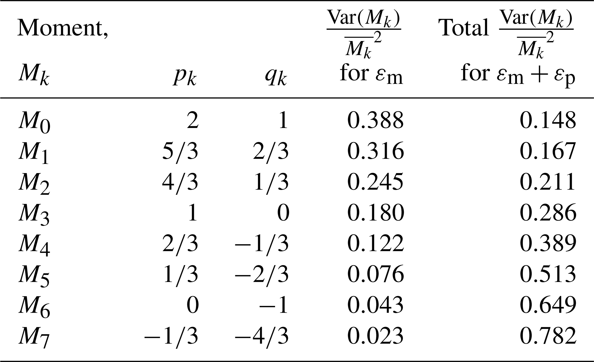
Using Eq. (A26), Table A1 gives the $\frac{\mathrm{Var}\left(M_k\right)}{{\stackrel{\mathrm{‾}}{M_k}}^{\mathrm{2}}}$ for radar measurement errors $\frac{\mathrm{Var}\left(M_{\mathrm{3}}\right)}{{\stackrel{\mathrm{‾}}{M_{\mathrm{3}}}}^{\mathrm{2}}}=\mathrm{0.18}$ and $\frac{\mathrm{Var}\left(M_{\mathrm{6}}\right)}{{\stackrel{\mathrm{‾}}{M_{\mathrm{6}}}}^{\mathrm{2}}}=\mathrm{0.043}$. From Sect. 4.2, the parameterization errors are $\frac{\mathrm{Var}\left(M_{\mathrm{3}}\right)}{{\stackrel{\mathrm{‾}}{M_{\mathrm{3}}}}^{\mathrm{2}}}=\mathrm{0.106}$ and $\frac{\mathrm{Var}\left(M_{\mathrm{6}}\right)}{{\stackrel{\mathrm{‾}}{M_{\mathrm{6}}}}^{\mathrm{2}}}=\mathrm{0.606}$. The total variances are obtained by adding these parameterization errors to the radar measurement errors, respectively, 0.18 and 0.043 to get 0.286 and 0.649. Thus, for ${\widehat{M}}_{\mathrm{6}}$ the parameterization error dominates with 93 % of the total variance, whereas for ${\widehat{M}}_{\mathrm{3}}$ the measurement error dominates with 63 % of the total. Using Eq. (A26) and total variances for ${\widehat{M}}_{\mathrm{3}}$ and ${\widehat{M}}_{\mathrm{6}}$ gives in Table A1 the total variances for the other moments. For M₀ through M₂, the total variance is smaller than the measurement variance because the covariance term is negative for those moments.

Table A1 Variance estimates for the radar-based retrievals of moments M₀ through M₇. The p and q are the exponents of $M_k=M_{\mathrm{3}}^p{M}_{\mathrm{6}}^{-q}$. The normalized variances due to measurement errors are given in the 4th column, while the totals due to measurement and parameterization errors are given in the 5th column.