the Creative Commons Attribution 4.0 License.
the Creative Commons Attribution 4.0 License.
 | 15 Sep 2020
Assessment of particle size magnifier inversion methods to obtain the particle size distribution from atmospheric measurements
Tommy Chan
Runlong Cai
Lauri R. Ahonen
Yiliang Liu
Ying Zhou
Joonas Vanhanen
Lubna Dada
Yongchun Liu
Markku Kulmala
Juha Kangasluoma
Accurate measurements of the size distribution of atmospheric aerosol nanoparticles are essential to build an understanding of new particle formation and growth. This is particularly crucial at the sub-3 nm range due to the growth of newly formed nanoparticles. The challenge in recovering the size distribution is due its complexity and the fact that not many instruments currently measure at this size range. In this study, we used the particle size magnifier (PSM) to measure atmospheric aerosols. Each day was classified into one of the following three event types: a new particle formation (NPF) event, a non-event or a haze event. We then compared four inversion methods (stepwise, kernel, Hagen–Alofs and expectation–maximization) to determine their feasibility to recover the particle size distribution. In addition, we proposed a method to pretreat the measured data, and we introduced a simple test to estimate the efficacy of the inversion itself. Results showed that all four methods inverted NPF events well; however, the stepwise and kernel methods fared poorly when inverting non-events or haze events. This was due to their algorithm and the fact that, when encountering noisy data (e.g. air mass fluctuations or low sub-3 nm particle concentrations) and under the influence of larger particles, these methods overestimated the size distribution and reported artificial particles during inversion. Therefore, using a statistical hypothesis test to discard noisy scans prior to inversion is an important first step toward achieving a good size distribution. After inversion, it is ideal to compare the integrated concentration to the raw estimate (i.e. the concentration difference at the lowest supersaturation and the highest supersaturation) to ascertain whether the inversion itself is sound. Finally, based on the analysis of the inversion methods, we provide procedures and codes related to the PSM data inversion.
- Article
(2241 KB) - Full-text XML
-
Supplement
(231 KB) - BibTeX
- EndNote


Gas-to-particle conversion proceeds via molecular clustering and subsequent cluster growth in various systems, such as atmospheric particle formation events, combustion processes or nanoparticle synthesis (Almeida et al., 2013; Carbone et al., 2016; Fang et al., 2018; Feng et al., 2015; Jokinen et al., 2018; Kulmala et al., 2004; Sipilä et al., 2016). Particle growth occurs at the size of a few nanometres, and direct measurements are presently available to probe the dynamics of the process. Instruments such as the diethylene glycol scanning mobility particle sizer (DEG-SMPS; Jiang et al., 2011a), the particle size magnifier (PSM, Airmodus Ltd., Finland; Vanhanen et al., 2011), the neutral cluster and air ion spectrometer (NAIS, Airel Ltd., Estonia; Mirme and Mirme, 2013) or the pulse height analysis condensation particle counter (PHA CPC; Marti et al., 1996) have been previously applied to directly measure the formation and growth of the clusters (Cai et al., 2017; Jiang et al., 2011b; Kontkanen et al., 2017; Manninen et al., 2010; Sipilä et al., 2009; Yu et al., 2017). These instruments have different operation principles and instrument functions; therefore, they require specific data inversion methods to obtain a reliable conversion from the measured (i.e. raw) data to a particle number size distribution. The SMPS, for instance, is a differential method that measures a narrow size band at one time (Stolzenburg and McMurry, 2008). The PSM, in contrast, is a cumulative method that measures total particle concentrations above certain threshold diameters (Cai et al., 2018). The comparison of the size distributions measured by these and some other instruments reveals that there is still work required to improve the accuracy of the measured sub-10 nm or sub-3 nm size distributions. Our focus in this study is the data inversion of the PSM for applications in atmospheric measurements.
Particle detection in the PSM is based on condensational growth of particles in two separate stages. In the first stage, the particles are grown with diethylene glycol (DEG) up to around 100 nm by mixing heated DEG vapour with a sample flow. In the second stage, the activated particles are further grown with butanol. The cut-off diameter (i.e. the diameter at which 50 % of the particles are activated in the first stage) varies between approximately 1 and 3 nm, depending on the mixing ratio of the DEG vapour. The mixing ratio is controlled by varying the flow rate that is saturated by DEG. Therefore, the raw data for the inversion problem consist of the measured total particle concentration above a certain cut-off diameter as a function of the flow rate through the saturator. Several parameters need to be considered in this specific inversion problem: (1) the shape of the cut-off curves (the instrument size function), (2) the data pre- and post-treatment to minimize random noise in the data, and (3) the mathematical method for the inversion.
To retrieve the sub-3 nm aerosol size distributions from the PSM raw data, the stepwise method and the kernel function method (Lehtipalo et al., 2014) have been used for the PSM data inversion of atmospheric measurements. The stepwise method is the promoted inversion method for commercial PSMs and is supported by Airmodus. It neglects the impact of the limited size resolution of the PSM on the measured aerosol concentration at each saturation flow rate and, therefore, causes systematic biases. The kernel function method considers the finite size resolution during inversion; however, it is more sensitive to random uncertainties than the stepwise method. To improve PSM inversion, Cai et al. (2018) compared four inversion methods: the stepwise method, the kernel function method, the Hagen–Alofs (H&A) method (Hagen and Alofs, 1983) and the expectation–maximization (EM) algorithm (Maher and Laird, 1985). It was suggested that the EM algorithm considers the finite size resolution and is less sensitive to random errors than the kernel function and H&A methods.
However, the study by Cai et al. (2018) was mainly based on theoretical simulations and well-controlled laboratory experiments. The larger measurement uncertainties associated with real atmospheric measurements compared with laboratory experiments may pose a challenge for each of these inversion methods. As indicated by Cai et al. (2018), the random uncertainty of the inverted size distribution is significant – even under a relative uncertainty of 10 % in the raw data. Furthermore, in contrast to laboratory experiments in which the detection efficiency for each particle size is known, the PSM detection efficiency of atmospheric aerosols is not determined due to their unknown chemical compositions. This unknown detection efficiency may also cause non-negligible biases (Kangasluoma and Kontkanen, 2017) to the inverted PSM data. As a result, the feasibility and performance of these inversion methods require further verification and testing using measured atmospheric data.
In this study, we present the four methods to invert measured atmospheric PSM data obtained in Beijing, China. We discuss the following aspects with respect to obtaining the particle size distribution: (1) the usability of individual scans; (2) the comparison of typical, inverted individual scans using the four inversion methods; (3) the characteristics of each inversion method when applied to atmospheric data; and (4) a simple method to determine, as a first approximate, the reliability of the inversion. Finally, based on the analysis of the performance of the inversion methods, we provide recommendations on how to invert atmospheric data measured with the PSM.
2.1 Site description
The study site is located on the fifth floor of the Aerosol and Haze Laboratory at the Beijing University of Chemical Technology, which is situated in the Haidan District in Beijing, China (39∘56′31′′ N, 116∘17′49′′ E; 58 m above sea level). The laboratory is near the third ring road of Beijing and gives a good representation of an urban environment that is surrounded by traffic, highways, and residential and commercial buildings. The combination of these different zones brings together pollution from local (e.g. traffic emissions and cooking) and longer-range sources.
This study was conducted between 15 January and 31 March 2018 (n=76 d) and was representative of a Beijing winter. Beijing winters are generally cold and dry with an average temperature of 0 ∘C. The average monthly temperature highs are 2, 5 and 12 ∘C, and the monthly lows are −9, −6 and 0 ∘C for January, February and March respectively. During these 3 months, the overall average humidity and rainfall are ∼44 % and 5.33 mm respectively.
2.2 Classification of event types
Three event types were identified for the study: new particle formation (NPF) events, haze events and non-event (i.e. neither haze nor NPF events). An NPF event is classified according to the method introduced by Dal Maso et al. (2005): the particle growth increases (in size) across different modes over several hours. Haze events were identified as days when the relative humidity was lower than 80 % and the visibility range was less than 10 km for a duration of 12 continuous hours. During the study period, we observed a total of 29 NPF events, 36 haze events and 11 non-events. NPF events were typically isolated as daily events that occurred after sunrise and continued into the early afternoon. Meanwhile, haze events occurred randomly throughout the day and could last for several days. These three event types did not commonly overlap with one another during the study period.
2.3 Aerosol particle measurements
Aerosol particle number concentration (expressed in particles cm−3) was measured using a butanol-based condensation particle counter (CPC; model A20, Airmodus Ltd., Finland). The CPC can measure a maximum particle concentration of up to 105 particles cm−3. The CPC is connected directly to the particle size magnifier (PSM; model A10, Airmodus Ltd., Finland). The PSM is a pre-conditioner for the CPC that uses diethylene glycol as the working fluid to activate and grow nano-sized particles (∼1–3 nm) so that they can be detected with the CPC (Vanhanen et al., 2011). A 1.3 m long horizontal inlet from where the aerosol particles entered was fixed to the PSM inlet, and a core sampler was fitted to reduce sampling line losses (Fu et al., 2019; Kangasluoma et al., 2016). Losses due to particle diffusion, penetration and core sampling were accounted for after the data inversion. If the sampling is done well (e.g. using a core sampler at the PSM inlet), the line losses can be negligible (Fu et al., 2019; Kangasluoma et al., 2016). If the losses are non-negligible but not large enough to decrease line penetration close to zero, the line losses can be corrected after the inversion for the size-classified data (e.g. using the size bin mean diameter). To maintain brevity, the term PSM will be used henceforth to refer to the PSM or the combination of the CPC and PSM.
The PSM measures the total particle concentration by mixing the sample aerosol flow with a heated saturated flow containing diethylene glycol. By varying the saturator flow rate, the mixing ratio of the sample flow and saturated flow changes; thus, the particle cut-off size can be changed. In other words, particles of specific diameters, assuming constant composition, will be activated and will grow to larger sizes based on the mixing ratio. In practice, the PSM can operate by scanning (i.e. incrementing and subsequently decrementing continuously) the saturator flow from 0.1 to 1.3 L min−1 in order to vary the particle cut-off size. For a constant particle size, the detection efficiency of the PSM as a function of the saturator flow rate is close to a sigmoid function, for which inversion methods that consider the instrument function are needed. In this study, we adjusted the duration of each scan to 240 s, recording data at 1 s intervals.
2.4 Data pre- and post-treatment
During the process of converting the measured data into a particle size distribution, the data were checked and treated prior to inversion (pretreatment) and following inversion (post-treatment). The programming language used for all data handling and data analyses was MATLAB version R2019a (The Mathworks, Inc.). Due to fluctuations in the air masses, the measured concentration as a function of the supersaturation is not always monotonically increasing, making the inversion procedure mathematically unsound. During periods when sub-3 nm particles are low, the measured concentration should theoretically be relatively constant as a function of the supersaturation. However, near the detection limit of the PSM, the inversion may face problems, which we will be explain in this study. Meanwhile, when the particle concentration is high, it is very possible that the concentration is real (Kangasluoma et al., 2020). Therefore, it is sensible to discard any scans not showing a positive correlation between the supersaturation and the measured concentration in order to avoid the inversion of any artificial counts from scans when there are clearly no sub-3 nm particles present – or if their presence is dubious.
The pretreatment included a data quality check and noise removal procedure. As there is a general, near-linear relationship between the saturator flow rate and measured concentration, the quality check employed a statistical hypothesis test (Spearman's rank correlation coefficient) for each scan that retained scans considered significant and positive, while discarding scans considered contrary to retained scans. Statistical significance was set at p<0.05 to consider subtle changes, which could be a real atmospheric influence. Following the significance test, a locally weighted scatterplot smoothing filter (LOWESS) was used over a span of 6 s for each single scan. The purpose of the smoothing was to minimize fluctuations or noise – for example, due to sudden changes in air mass. We explored the performance of the pretreatment quality scan, especially pertaining to what scans were retained and discarded. In addition, we applied each inversion method to these retained and discarded scans to further understand the inversion process. A smoothing average over two scans (i.e. 8 min in this study) was applied after the inversion. This reduced the random uncertainty in the inverted data and facilitated, for example, the calculation of particle growth and formation rates. Note that another noise-filtering mechanism (e.g. median filtering) could be used, depending on the user's discretion. The smoothing is carried out after rather than before the inversion because the measured concentration is autocorrelated, whereas the inverted size distribution is simply a function of particle diameter and, therefore, can be averaged for the same size bin.
2.5 Data inversion
In this study, four inversion methods were tested using data obtained via atmospheric measurements: the stepwise method (Lehtipalo et al., 2014), the kernel function method (Lehtipalo et al., 2014), the Hagen–Alofs method (H&A; Hagen and Alofs, 1983) and the expectation and maximization algorithm (EM; Dempster et al., 1977; Maher and Laird, 1985).
The particle number concentration measured with the PSM uses the Fredholm integral equation of the first kind to determine the particle size distribution:
where Ri is the raw concentration for a saturator flow rate of si; η is the detection efficiency calculated from s and Dp; Dp is the particle size; n(dDp) is the particle size distribution function (in particles cm−3 nm−1); and εi represents the errors in the measurement at si. For atmospheric measurements, the relatively large εi poses a challenge with respect to data inversion. For example, when the detection efficiency is high, the PSM will record measurement background. Meanwhile, low concentrations recorded from the PSM can also contribute to these errors.
The stepwise method is currently the proprietary inversion method for use with the PSM. When calculating particle size distributions using the stepwise method, the size resolution of the PSM is assumed to be infinite (i.e. the kernel function is approximated with a Dirac delta function whose area is equal to the real kernel but whose height is infinite). Based on this assumption, it can be demonstrated that there is a one-to-one relationship between the saturator flow rate and the activated particle diameter; hence, the particle number concentration in the specific size range can be obtained by calculating the measured particle number concentration increment (after correcting the detection efficiency) in its corresponding saturator flow rate range. The expression for the stepwise method, introduced in Lehtipalo et al. (2014) in practical use, is as follows:
where nm is the particle size distribution (dN∕dDm) at diameter Dm; Dm is the median diameter of Di and Di+1; Di and Di+1 are the corresponding diameters of the saturator flow rates si and si+1 respectively, and this one-to-one relationship is obtained based on the infinite-resolution assumption; Ri and Ri+1 are the raw concentration recorded by the PSM after the dilution has been corrected for; smax is the maximum saturator flow rate; and η is the PSM detection efficiency at the given saturator flow rate and particle diameter. The inverted dN∕dDm was later converted into dN∕dlog Dm. The derivation of the stepwise method is given in the Supplement.
The kernel function and H&A methods both account for the kernel functions of the PSM. At each saturator flow rate, the measured total particle number concentration (or its derivative with respect to the saturator flow rate) is equal to the sum of particle number concentrations in each size bin multiplied by their detection efficiencies (or corresponding kernel functions). The particle number concentrations in each size bin are obtained by solving the non-homogeneous, linear equations that relate saturator flow rates and particle number concentrations. The difference between the kernel function and H&A methods is the number of assumed particle size bins. The kernel function method uses a size bin number (typically four to six) that is much lower than the number of saturator flow rates, whereas the H&A method uses a size bin number (theoretically infinite) that is much higher than the number of saturator flow rates and then reduces the size bin number to the saturator flow rate number using predetermined interpolation functions. Note that the H&A method itself does not specify that the detection efficiencies or the kernel functions should be used for data inversion. In this study, detection efficiencies are used in the H&A method to avoid the introduction of uncertainties when estimating the derivate of the particle number concentration with respect to the saturator flow rate as well as to remain in accordance with Cai et al. (2018).
The EM algorithm is an iterative algorithm based on the theories of probability that is used in the inversion of diffusion batteries (Maher and Laird, 1985; Wu et al., 1989) and machine learning (e.g. Erman et al., 2006). The expressions for the EM algorithm are as follows:
where I is the total number of saturator bins, and the ith saturator flow rate is si; J is the total number of particle size bins, and the jth particle size is Dj; ΔDj is the width of the jth size bin; nj is the particle size distribution at Dj (dN∕dDj); η is the PSM detection efficiency for the given si and Dj; and Ri, j is the contribution of the jth size bin to the total raw concentration (Ri) measured at si, and it is a latent variable that cannot be directly measured. Similar to the H&A method, J should theoretically be infinite to avoid integral error caused by the limited number of size bins, and it is practically determined as 50 in this study. For additional details on the four inversion methods, refer to previous studies (Cai et al., 2018; Hagen and Alofs, 1983; Lehtipalo et al., 2014; Maher and Laird, 1985).
2.6 Data analysis
From a total study duration of 76 d, we selected a total of 12 d for in-depth analysis: 4 NPF event days, 4 haze days and 4 non-event days. For the convenience of comparison, the aerosol size distributions from each of the inversion methods are reported in 6 and 11 size channels, indicated by 7 and 12 limiting diameters of the size channels respectively. The 6-channel distribution consisted of the following sizes: 1.2, 1.3, 1.5, 1.7, 2.0, 2.5 and 2.8 nm. Moreover, the shape of the kernel was approximated using a Gaussian distribution, based on the calibration file (see Sect. 3.1). The 11-channel distribution consisted of the following sizes: 1.2, 1.3, 1.4, 1.5, 1.6, 1.7, 1.8, 1.9, 2.0, 2.1, 2.5 and 2.8 nm. The 11-channel inversion was shown to be very similar to the 6-channel inversion (see Fig. S1 in the Supplement); however, with the exception of the illustration of the data inversions of single scans (i.e. Fig. 1), the 6-channel distribution was used in this study, as it is a commonly used size bin range and the six kernel function peaks do not significantly overlap with each other (see Fig. S2 in the Supplement). For the stepwise method, the total particle concentrations measured at the seven saturator flow rates were inverted into aerosol size distributions at six particle sizes using Eq. (2). For the kernel function method, the measured particle concentration as a function of the saturator flow rate was inverted to six size bins using the least squares method. For the H&A method and the EM algorithm, the size distribution was first inverted into 50 size channels and then reduced to 6 channels by merging adjacent channels. Assuming that there is no error or uncertainty in the kernel functions and particle aerosol number concentration recorded by the PSM, the inversion methods should be able to distinguish more particle size channels – even if their kernel function peaks overlap with one another or if the size resolution is limited. However, considering the fact that the atmospheric instability and its particle composition is unknown, we report the size distributions in six channels in this study.
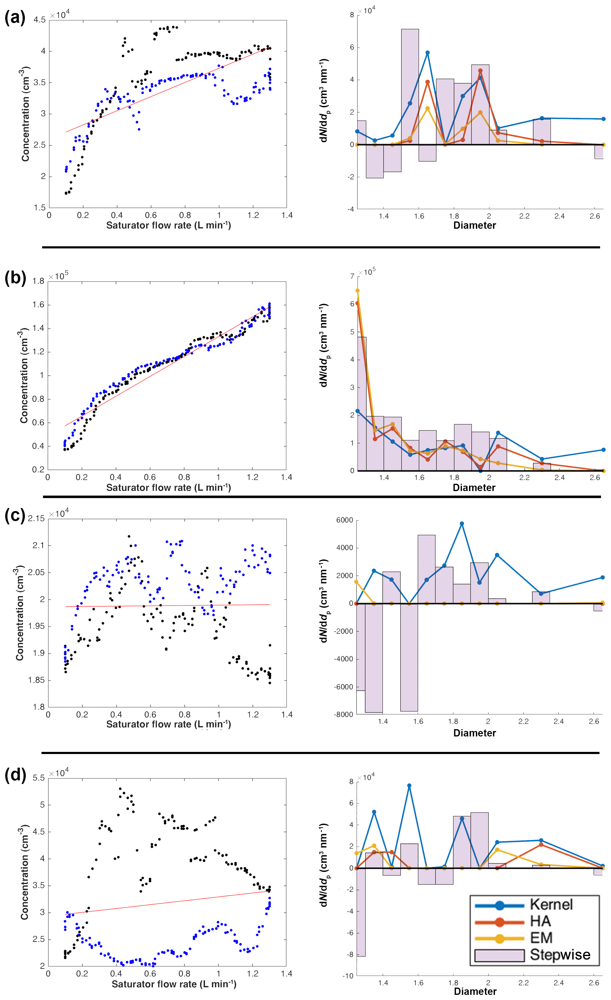
Figure 1The 4 min retained (a, b) and discarded (c, d) scans using the PSM (left column) and their inversion into a particle size distribution (right column). The black dots indicate the (2 min) upward scan of the saturator flow, and the blue dots indicate the corresponding (2 min) downward scan of the saturator flow. The red line indicates the regression line of the 4 min scan. An 11-channel size bin range was used for the inversion.
The general challenge in the current sub-3 nm atmospheric size distribution measurements is that there is no real reliable reference with which to compare size distributions. In some recent experiments, there has been a concurrent SMPS-based measurement with the PSM (e.g. Kangasluoma et al., 2020); however, this only gives another independent estimate of the size distribution. Therefore, as a basis for comparison between each inversion method, we compared the integrated total concentration from the inverted distribution to the estimated raw concentration between the mobility diameters of 1.2 and 2.8 nm, R1.2−2.8. This is calculated as the difference between the total particle concentrations measured at the lowest and highest saturator flow rates (i.e. 0.1 and 1.3 L min−1 respectively). From this comparison, R1.2−2.8 should be approximately equal to the concentration integrated in the same size range from the inverted size distribution. While the comparison is not expected to yield exact quantitative agreement, it provides an idea of whether the inverted concentration is reasonable, especially during periods when few or no sub-3 nm particles are present. Moreover, this comparison can ensure that the data are internally consistent.
As an additional analysis, we performed a signal-to-noise ratio calculation to determine the detection limit of the PSM from the four inversion methods. In short, the calculation allows the user to identify where the possible noise and measured concentration converge. This is especially important to identify the smallest concentration that the inversions allows (which varies between the PSM instruments and sample site). The signal-to-noise ratio is calculated by dividing the integrated concentration from the whole size range by the total concentration measured at the cut-off of 0.1 L min−1. It is important to note, however, that the term “noise” is difficult to define, as noise could arise from the data or from the instrument itself.
The general workflow to obtain the particle size distribution using the PSM was as follows:
-
determine whether the estimated kernel function curves are reasonable;
-
pretreat the data to remove scans with no statistical significance;
-
select a filtering method to remove random noise in the measurements
-
invert the measurement data;
-
correct data for losses;
-
apply a post-inversion filtering method;
-
compare the inversion to R1.2−2.8 to check the reliability of the inversion.
In the following sections, we will first discuss the kernel function curves, followed by data pretreatment – especially the criterion to retain and discard scans. Following that, an overview of the four inversion methods applied to the three event types will be given. These results will be inter-compared based on the sum of the inverted aerosol concentration and the aerosol size distributions in each size bin.
3.1 Estimating the kernel function curves
In short, the estimated kernel function curves are the derivative of the detection efficiency curves. As the growth tube and the temperature of the saturator of the PSM do not change, a higher saturator flow rate will result in a higher supersaturation ratio of DEG in the growth tube, resulting in higher detection efficiencies. This result is inversed when the saturator flow rate is lower. The particle diameter cut-off sizes (taken at 50 % detection efficiency) can be obtained from the calibration file provided by Airmodus Ltd. or by classifying charged particles with the use of a high-flow differential mobility analyser. For further insight into obtaining the detection efficiency curves, refer to Cai et al. (2018). As the kernels are derived under laboratory conditions, it is important to note that the kernels may not be directly accurate when measuring atmospheric particles due to the unknown chemical composition; nevertheless, they should be mathematically self-consistent, i.e. the corresponding detection efficiency increases with increasing particle diameter and saturator flow rate and the detection efficiency for large particles (e.g. 10 nm) does not vary in the saturator flow rate range used.
3.2 Data retention rate and pre-inversion treatment
Table 1 presents the total number of daily scans (from 00:00 to 23:59 LT, local time), and the number of retained and discarded scans. The test showed that both non-event and NPF events had a retention rate of over 90 %, whereas haze events revealed an 80 % retention rate. Of the three specific non-event days chosen, two had a high retention rate, while one had as many discarded scans as a haze event. A typical example of a measured 4 min scan can be seen in Fig. 1. Retained scans (Fig. 1a, b) revealed a good correlation between the saturator flow rate and the measured particle concentration. In addition, the Spearman's rank correlation coefficient (ρ) of each retained scan was also significant. This contrasted with discarded scans (Fig. 1c, d), which showed an insignificant ρ value and no correlation between the saturator flow rate and the particle concentration.
Table 1List of selected days for analysis, including their event type, the number of scans and the retention rate. All data were measured in 2018.
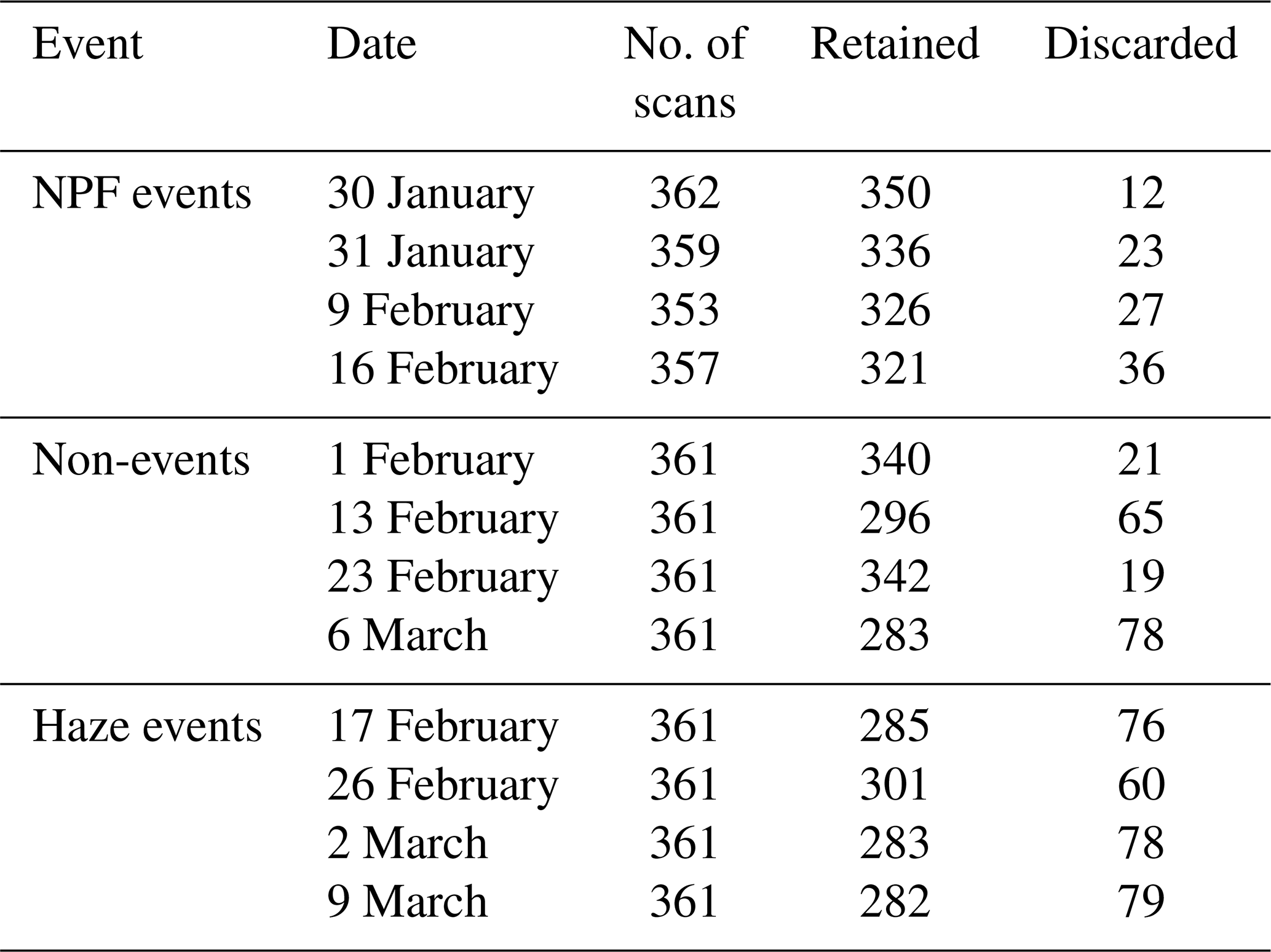
High retention rates may indicate the presence of sub-3 nm particles, whereas lower retention rates, such as during haze days, may indicate that less sub-3 nm particles are present. As the aim is to invert high-quality scans, only the scans with no significant correlation or a negative correlation between the measured concentration and the saturator flow rate are discarded; hence, the retention rate is around 80 % even during haze days. However, the presence of sub-3 nm particles even in the presence of a high condensation sink also contribute to this high ratio of 80 %, as discussed further in this study. Figure 1c and d also present a typical challenge where the time resolution of the instrument (4 min in this case) is larger than the timescale of the variations in the measured aerosol. High variations in the number concentration during one scan oftentimes makes it difficult to reliably invert data from a cumulative instrument, and, indeed, the presented retention criteria may discard a large proportion of the scans that are mathematically difficult to invert.
3.3 Scan inversion
Individual, 4 min scans of both retained and discarded scans were inverted using the four inversion methods in order to assess the quality of the inversion and of the scan itself (Fig. 1). A measurable difference between retained and discarded inverted scans was observed. The inverted, discarded scans revealed concentrations close to zero for each size bin of each method, whereas the inverted, retained scans revealed a quantifiable size distribution. From these inversions, one can make a few observations; for example, all inversion methods give a rather similar-looking inverted size distribution for the retained scans, which suggests that all methods result in a reasonable inversion if the obtained raw data are good, which is in line with previous laboratory measurements by Cai et al. (2018). Certainly, the data quality check prior to data pretreatment would ensure that the raw data that are considered good are retained, whereas the bad data is filtered out. The exception to this is the stepwise method, which is sensitive to the slight air mass fluctuations that may lead to negative inverted or erroneous concentrations in some size bins. In the selected examples of the discarded scans (Fig. 1c, d), the kernel and stepwise methods' inverted concentrations yielded a particle size distribution despite the scan suggesting that there were no signals from sub-3 nm particles. As indicated above, the observed concentration fluctuations may have originated from air mass fluctuations. This means that, with the measurement uncertainties, the use of the stepwise and kernel methods without prior data checking may lead to the inversion of artificial particle concentrations that are only revealed during the inversion. In contrast, the H&A and EM methods appear to be much more robust against noisy data; after the inversions, these methods yielded no concentrations at all from the discarded scans. The significant differences in the behaviour of these inversion methods revealed measurement uncertainties that agree with the findings of Cai et al. (2018), which were based on a Monte Carlo simulation.
3.4 Comparison of inversions to R1.2−2.8 and total concentration
The inverted dataset was compared with R1.2−2.8 values from the same size range in order to estimate how well the inverted data were represented (Fig. 2). The variable R1.2−2.8 is calculated as the particle concentration difference between the saturator flow rate at 1.3 and 0.1 L min−1. The sub-3 nm particle concentration estimate based on R1.2−2.8 is more reliable when the sub-3 nm particle concentration is larger relative to the background particle concentration (i.e. all the particles outside of the PSM sizing range, which in this study was n>2.8 nm). If the ratio is low, the sub-3 nm particle concentration signal might not be distinguishable from the fluctuations in the background concentration. Further, as there are no corrections in the R1.2−2.8 concentration estimate (e.g. losses), it might underestimate the real sub-3 nm particle concentration. During NPF events, the stepwise inversion method reported the highest concentrations – about a factor of 2 larger than the kernel method, which showed the lowest concentrations. The H&A and EM methods reported concentrations that were between the stepwise and the kernel method and that closely resembled the concentration obtained from R1.2−2.8. During non-NPF and haze periods, when R1.2−2.8 was very noisy, the kernel method clearly revealed the highest concentrations, which were likely due to overestimation. This can be observed in Fig. 1, where the concentrations inverted using the kernel method are clearly inversion artefacts from scans that were discarded based on the insignificant correlation between the saturator flow rate and the measured particle concentration. The stepwise, EM and H&A methods showed rather similar concentrations, which were quite close to the values obtained from R1.2−2.8 estimates. An interesting observation was made during NPF events: the H&A and EM methods revealed very little to no particle concentration before and after the NPF, which is contrary to what the kernel and stepwise methods and the R1.2−2.8 estimates reported. This could also be observed during haze and non-event periods, but the differences were more subtle compared with the other inversion methods and with R1.2−2.8.

Figure 2Comparison between inverted and raw data (i.e. R1.2−2.8; calculated as the difference between the saturator flow rate at 1.3 and 0.1 L min−1). The event types shown are (a) a NPF event on 30 January 2018, (b) a non-event on 6 March 2018 and (c) a haze event on 9 March 2018.
To gain further insight into the overall performance of the inversions when the sub-3 nm particle concentration is low, histogram plots were made of the integrated concentration from the whole size range that is normalized with the total concentration measured at the cut-off of 2.8 nm (0.1 L min−1; Fig. 3). The following observations can be made: the stepwise method is not sensitive to the concentrations because it is direct subtraction of concentrations; thus this may yield negative concentrations. The H&A and EM methods report high frequency at ∼0 as well as elevated frequencies below ratios less than 0.015 (or on an absolute scale, less than about 200 cm−3). This is in line with Cai et al. (2018), who show that the H&A and EM methods tend to report a near-zero size distribution when the sub-3 nm particle concentration is noisy and low compared with the background aerosol concentration. In contrast, the kernel method never revealed ratios smaller than 0.015, which can be explained according to Fig. 1c and d – even when inverting data that clearly do not contain a signal from sub-3 nm particles, the kernel method inverted some artificial particle concentrations. These artificial inverted concentrations originate from the random noise in the data that the inversion methods interpret as a real signal.
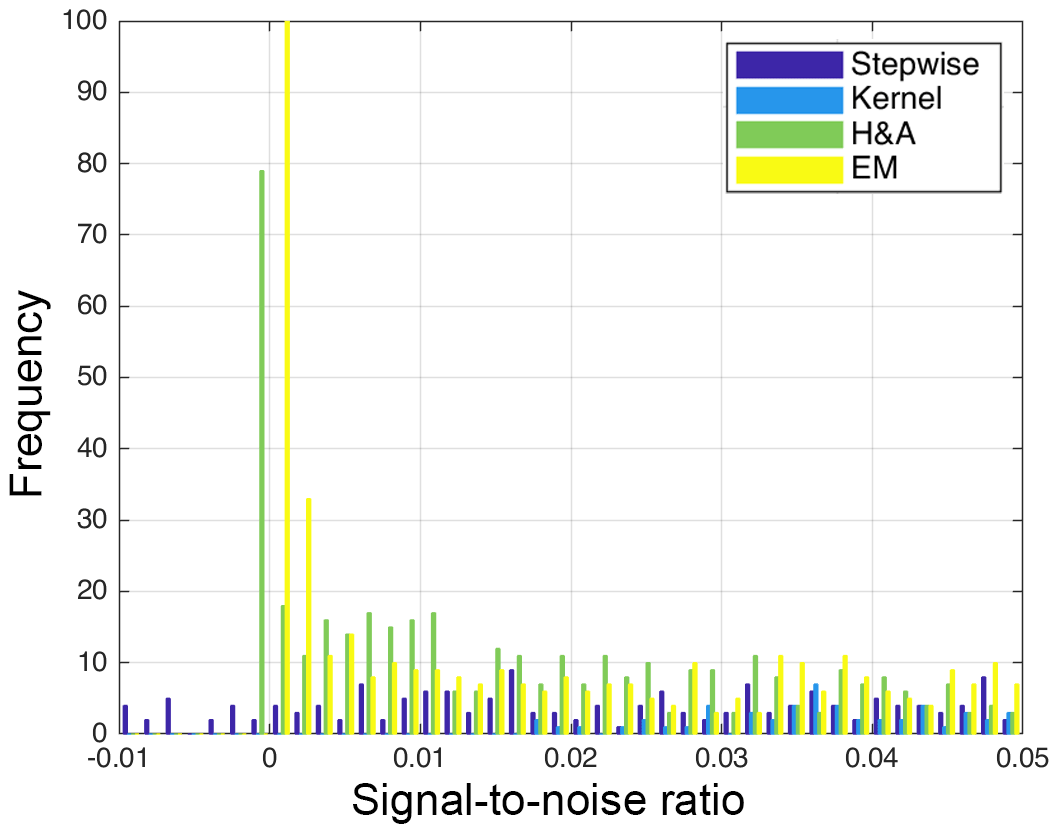
Figure 3Signal-to-noise ratio of all selected study days. Data shown are the integrated concentrations from the whole size range with the total concentration measured at the cut-off of 2.8 nm (0.1 L min−1).
3.5 Overview of the inversion for different types of events
3.5.1 New particle formation (NPF) events
All NPF events in the study showed a typical increase in the particle concentration, with the highest concentrations observed around noon and the lowest concentrations observed at night (Fig. 4). All of the methods revealed that the highest concentrations were observed in the smallest size bin. The EM, H&A and kernel methods revealed high concentrations in the largest size bin. Both the EM and H&A methods showed very similar concentrations to one another. In contrast to the EM and H&A methods, the kernel and stepwise methods revealed a larger total concentration outside of the NPF event, and the concentration intensity revealed no identifiable pattern. As discussed above, the difference is mainly caused by the behaviour of these inversion methods at a low signal-to-noise ratio.
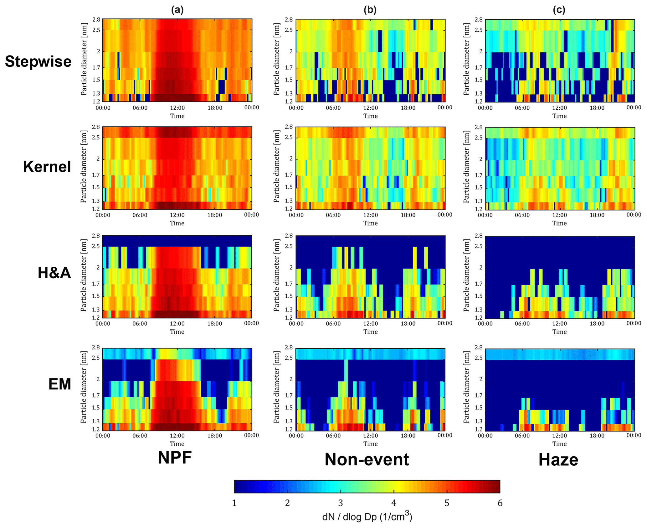
Figure 4The stepwise, kernel, H&A and EM inversions of (a) a selected NPF event on 30 January 2018, (b) a non-event on 6 March 2018 and (c) a haze event on 9 March 2018.
3.5.2 Non-events
During non-event days, there was no indication of NPF events (Fig. 4). The distribution of the EM and H&A methods looked similar to one another compared with the kernel and stepwise methods. In addition, the H&A and EM methods revealed no particle sizes larger than 2 nm between 00:00 and 06:00 LT and between 12:00 and 18:00 LT, which largely contrasted with the kernel and stepwise inversion methods. The stepwise method revealed scattered gaps with zero particle concentrations in the size bins covered by the PSM throughout the day. This may be due to the limitation of the stepwise inversion algorithm. As the algorithm is calculated as the difference between two adjoining size bins, if the difference is revealed to be negative, the inversion itself would then have a gap in the size distribution. These gaps are more evident during noisier periods, such as during haze events and non-events. In contrast, the size distributions are latently smoothed in the H&A and EM methods.
3.5.3 Haze events
Similar to non-event days, during haze events the kernel and stepwise methods revealed particle concentrations in all size ranges throughout the day, whereas the H&A and EM methods showed concentrations predominantly in the lower size range. This led to the latter two methods being more qualitatively discernible compared with the kernel and stepwise methods. As with the other events, the EM method had large concentrations of particles in the highest size bin.
3.6 Comparison of inversion size bins
To compare the single size bins of each inversion method, four size bins were selected: 1.2–1.3, 1.5–1.7, 1.7–2.0 and 2.0–2.5 nm (Fig. 5). Three days were chosen to represent NPF, non-event and haze days (see also Figs. 2 and 4). During the NPF event, all the four inversion methods captured the diurnal trend of the particle size distribution initiated by NPF. Considering measurement uncertainties, the inverted size distributions from different inversion methods generally agreed well with each other, although the kernel method reported a much lower overall size distribution. As seen from Fig. 2, the kernel method inversion clearly underestimated the NPF event particle size distribution and is also revealed in Fig. 5 in all but the largest size bin. Meanwhile, the stepwise method reported higher aerosol size distributions compared with the H&A and EM methods. Although the particle concentrations in the 1.2–1.3 nm channel were very similar, the difference in measured concentration was attributed to other sizes – particularly between 1.5 and 2.0 nm. The largest size bin (2.0–2.5 nm) revealed an interesting observation: both EM and H&A had lower concentrations than the stepwise and kernel methods. The latter two methods on 30 January showed a small peak at 07:00 LT, which would be the approximate time that the NPF event began(as seen in Fig. 2). It should be clarified that the true kernel functions are not determined due to the unknown aerosol chemical compositions. Hence, the differences between the inversion results may sometimes reflect the uncertainty of the measurement itself rather than quantifying the difference between the inversion methods.
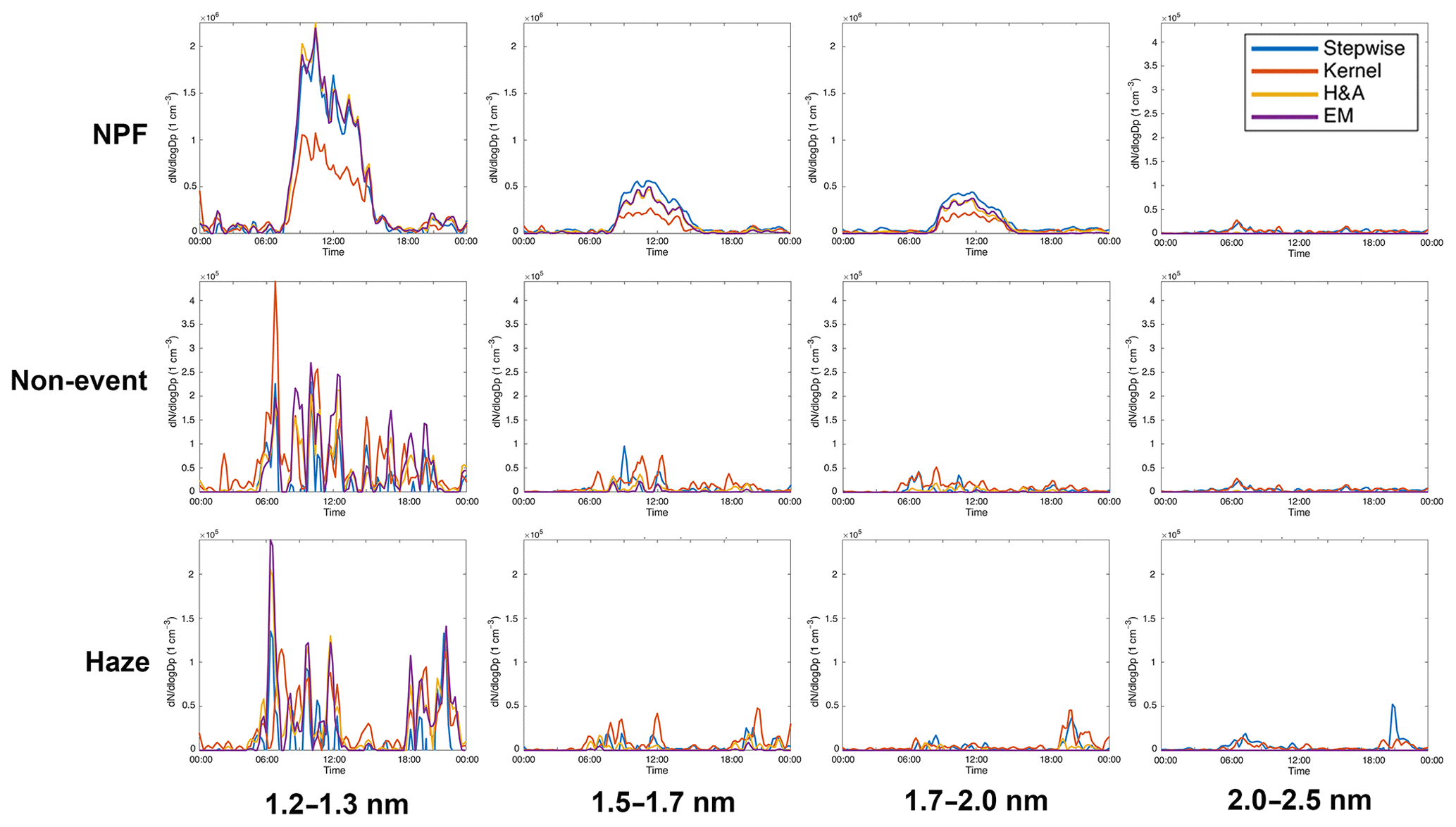
Figure 5Comparison of size bins from inversions. Event types shown are an NPF event on 30 January 2018 (top row), a non-event on 6 March 2018 (middle row) and a haze event on 9 March 2018 (bottom row).
During non-event and haze periods, newly formed clusters and particles are scavenged over a short period of time under the high coagulation sink in urban Beijing, and their concentrations are presumably low (Cai et al., 2019). The EM method reported near-zero concentrations above 1.7 nm, because it tends to report near-zero values when the particle concentration is low and noisy, as discussed in Sect. 3.3. In contrast, the stepwise and kernel methods reported constantly present concentrations for particles larger than 1.7 nm. A similar phenomenon was also observed during the midnight hours of the NPF event. The methodological biases, such as the infinite-resolution assumption of the stepwise method and the instability of the least squares method used in the kernel and H&A methods, are the major causes of the background. Although the methods each revealed inversion challenges with measured atmospheric data, it is important to note that the inversion methods were rather robust in chamber studies (e.g. Cai et al., 2018).
In this study, we assessed the performance of four inversion methods: the stepwise method, the kernel method, the H&A method and the EM algorithm to invert PSM data measures under real, atmospheric conditions. In addition, the study presented a novel method to pretreat the data prior to inversion. The presented data employed a pretreatment filter that scans the measured data to calculate the correlation between the observed particle concentration and the supersaturation of a single scan. From the correlation analysis, scans are discarded when there is a significant noncorrelation or negative correlation. The performance of the respective inversion methods was assessed by inverting single scans. All of the methods were found to perform relatively well for scans that were measured during NPF events, although the inverted size distributions were overestimated with the kernel method when the data were noisy (i.e. during non-event or haze periods), and negative values could be obtained with the stepwise method when inverting noisy data. The EM and H&A methods were more robust when inverting noisy data, which, in these cases, reported zeros. As the variations in the background particle concentrations affected the performance of the inversion methods, one should be cautious when using any of these methods to approximate a size distribution when the total measured concentration and signal-to-noise ratio are low (less than ∼500 cm−3 and ∼0.02 respectively in our study).
Based on the analysis presented in this study, there are many considerations that the user must be aware of when inverting PSM data:
-
When inverting PSM data, a good guideline to follow is to first create a similar workflow to that used in this study (see Sect. 2.6). Ideally, users should stop between each step to examine the data output to ensure that it looks reasonable before continuing. This way, users will know where, during the inversion process, the problem lies.
-
Selection of the size channels for inversion is important and largely depends on the instrument-specific calibration. First, the channels need to fall within the calibration curve limits, and each size diameter limit has to have its own distinct saturator flow. The latter is especially important because the saturator flow vs. diameter (calibration) curve begins to flatten out at diameters greater than 2 nm.
-
Data pretreatment is an important part of the inversion to obtain reliable data. Scans that contain a clearly unphysical correlation between the measured concentration and the supersaturation should be discarded. An unphysical correlation is one where the saturator flow rate of the PSM is not positively correlated with the measured total concentration. We employ a Spearman's rank correlation coefficient with a significance set at p<0.05 to ensure that data are of a high quality. Naturally, changing this significance threshold would yield stricter or more relaxed restrictions, likely resulting in fewer or more retained scans respectively.
-
In this paper, we used 4 min scans (i.e. the combination of an upward and downward scan of the saturator flow) as the time resolution of our measurements. Alternatively, scans can be selected at a higher 2 min resolution or at lower resolutions (i.e. >4 min scan). The selection of the scanning length is a compromise between better quality data and a higher time resolution. In our case study, we measured urban atmospheric particles where growth rates at this size range can be approximately 1 nm h−1. Therefore, selecting 4 min scans is a reasonable time resolution.
-
It is strongly advised to invert the data with more than one inversion method in order to be able to compare the results, rather than blindly accepting the inverted values of one method. A comparison would affirm whether the inverted measured concentration is real and whether they are in good agreement (e.g. within a factor of 0.5–2; see point 7, below). If the comparison does not agree, the user should check that the kernel function curves are reasonable (see Cai et al., 2018).
-
The recommended method to retrieve the particle size distribution of PSM data is the EM method. From this study, the EM and H&A performed similarly; however, based on theoretical understanding (see Cai et al., 2018), the EM method is the more stable of the two (i.e. the inversion is smoother and the concentration is more continuous). The kernel method should not be used to invert PSM data during non-NPF events and should be used cautiously during NPF events. This is because inversions may be over- or underestimated, and, at worst, artificial counts can be created by the inversion itself.
-
The measured size distributions of ambient aerosols should be reported using a limited number of size bins (e.g. four to six channels), because the assumed inversion kernels may deviate from the true kernels.
-
To improve data reliability, comparability and availability, the inversion method and the measured size distribution functions (dN∕dlog Dp vs. Dp) used should be reported along with any other subsequent analysis from the PSM data.
-
As a first approximation, the PSM user should compare the inverted total sub-3 nm particle concentration to the sub-3 nm concentration obtained from the raw data by subtracting the concentration measured at the lowest supersaturation from the concentration measured at the highest supersaturation (R1.2−2.8). These concentrations should be comparable (within a factor of 0.5–2). However, if the inverted data do not correspond well with R1.2−2.8, they should be checked using other inversion methods – the deviation may be due to the inversion or poor-quality data.
-
A signal-to-noise ratio test can be performed to determine the smallest concentration that can be detected with the PSM. This would help users identify the measurement limits of the instrument from the data. In our study, we found that the site-specific ratio was approximately 0.02. Nevertheless, as a safety limit, we advise users to use data 2–3 times higher than their calculated ratio.
-
Most importantly, the performance of the PSM should be checked regularly, and the detection efficiency (that determines the inversion kernel) should be calibrated sporadically because the kernel information is used in the EM, H&A and kernel inversions.
-
The MATLAB code written for this study as well as sample atmospheric data and the PSM calibration file are available via GitHub (https://github.com/tommychan-dev/PSM-Inversion, last access: 17 January 2020).
The MATLAB inversion codes used for this study are available via GitHub (https://github.com/tommychan-dev/PSM-Inversion, last access: 17 January 2020, Chan, 2019).
The supplement related to this article is available online at: https://doi.org/10.5194/amt-13-4885-2020-supplement.
TC, RC and JK designed the study, and TC carried it out. TC, RC, LRA, JV and LD developed the inversion code. YL (Fudan), LW, YZ, YC, YL (BUCT) and MK provided the facilities, instruments and funding for the study. TC prepared the paper with contributions from all co-authors.
The authors declare that they have no conflict of interest.
We wish to thank Rima Baalbaki for her insightful comments and code debugging prowess.
This research has been supported by the University of Helsinki, Faculty of Science (grant nos. 75284140 and 75284132) and the Finnish Academy of Science (grant no. 1325656).
Open access funding has been provided by the Helsinki University Library.
This paper was edited by Charles Brock and reviewed by two anonymous referees.
Almeida, J., Schobesberger, S., Kürten, A., Ortega, I. K., Kupiainen-Määttä, O., Praplan, A. P., Adamov, A., Amorim, A., Bianchi, F., Breitenlechner, M., David, A., Dommen, J., Donahue, N. M., Downard, A., Dunne, E., Duplissy, J., Ehrhart, S., Flagan, R. C., Franchin, A., Guida, R., Hakala, J., Hansel, A., Heinritzi, M., Henschel, H., Jokinen, T., Junninen, H., Kajos, M., Kangasluoma, J., Keskinen, H., Kupc, A., Kurtén, T., Kvashin, A. N., Laaksonen, A., Lehtipalo, K., Leiminger, M., Leppä, J., Loukonen, V., Makhmutov, V., Mathot, S., McGrath, M. J., Nieminen, T., Olenius, T., Onnela, A., Petäjä, T., Riccobono, F., Riipinen, I., Rissanen, M., Rondo, L., Ruuskanen, T., Santos, F. D., Sarnela, N., Schallhart, S., Schnitzhofer, R., Seinfeld, J. H., Simon, M., Sipilä, M., Stozhkov, Y., Stratmann, F., Tomé, A., Tröstl, J., Tsagkogeorgas, G., Vaattovaara, P., Viisanen, Y., Virtanen, A., Vrtala, A., Wagner, P. E., Weingartner, E., Wex, H., Williamson, C., Wimmer, D., Ye, P., Yli-Juuti, T., Carslaw, K. S., Kulmala, M., Curtius, J., Baltensperger, U., Worsnop, D. R., Vehkamäki, H., and Kirkby, J.: Molecular understanding of sulphuric acid–amine particle nucleation in the atmosphere, Nature, 502, 359–363, https://doi.org/10.1038/nature12663, 2013.
Cai, R., Yang, D., Fu, Y., Wang, X., Li, X., Ma, Y., Hao, J., Zheng, J., and Jiang, J.: Aerosol surface area concentration: a governing factor in new particle formation in Beijing, Atmos. Chem. Phys., 17, 12327–12340, https://doi.org/10.5194/acp-17-12327-2017, 2017.
Cai, R., Yang, D., Ahonen, L. R., Shi, L., Korhonen, F., Ma, Y., Hao, J., Petäjä, T., Zheng, J., Kangasluoma, J., and Jiang, J.: Data inversion methods to determine sub-3 nm aerosol size distributions using the particle size magnifier, Atmos. Meas. Tech., 11, 4477–4491, https://doi.org/10.5194/amt-11-4477-2018, 2018.
Cai, R., Jiang, J., Mirme, S., and Kangasluoma, J.: Parameters governing the performance of electrical mobility spectrometers for measuring sub-3 nm particles, J. Aerosol Sci., 127, 102–115, https://doi.org/10.1016/j.jaerosci.2018.11.002, 2019.
Carbone, F., Attoui, M., and Gomez, A.: Challenges of measuring nascent soot in flames as evidenced by high-resolution differential mobility analysis, Aerosol Sci. Tech., 50, 740–757, https://doi.org/10.1080/02786826.2016.1179715, 2016.
Chan, T.: PSM-Inversion, GitHub, available at: https://github.com/tommychan-dev/PSM-Inversion (last access: 17 January 2020), 2019.
Dal Maso, M., Kulmala, M., Riipinen, I., Wagner, R., Hussein, T., Aalto, P. P., and Lehtinen, K. E.: Formation and growth of fresh atmospheric aerosols: eight years of aerosol size distribution data from SMEAR II, Hyytiälä, Finland, Boreal Env. Res., 10, 323–336, 2005.
Dempster, A. P., Laird, N. M., and Rubin, D. B.: Maximum likelihood from incomplete data via the EM algorithm, J. Roy. Stat. Soc. B Met., 39, 1–22, https://doi.org/10.1111/j.2517-6161.1977.tb01600.x, 1977.
Erman, J., Mahanti, A., and Arlitt, M.: Qrp05-4: Internet Traffic Identification using Machine Learning, in: IEEE Globecom 2006, San Francisco, CA, USA, 27 November–1 December 2006, IEEE, 1–6, https://doi.org/10.1109/GLOCOM.2006.443, 2006.
Fang, J., Wang, Y., Kangasluoma, J., Attoui, M., Junninen, H., Kulmala, M., Petäjä, T., and Biswas, P.: The initial stages of multicomponent particle formation during the gas phase combustion synthesis of mixed SiO2∕TiO2, Aerosol Sci. Tech., 52, 277–286, https://doi.org/10.1080/02786826.2017.1399197, 2018.
Feng, J., Huang, L., Ludvigsson, L., Messing, M. E., Maisser, A., Biskos, G., and Schmidt-Ott, A.: General approach to the evolution of singlet nanoparticles from a rapidly quenched point source, J. Phys. Chem. C, 120, 621–630, https://doi.org/10.1021/acs.jpcc.5b06503, 2015.
Fu, Y., Xue, M., Cai, R., Kangasluoma, J., and Jiang, J.: Theoretical and experimental analysis of the core sampling method: Reducing diffusional losses in aerosol sampling line, Aerosol Sci. Tech., 53, 793–801, https://doi.org/10.1080/02786826.2019.1608354, 2019.
Hagen, D. E. and Alofs, D. J.: Linear inversion method to obtain aerosol size distributions from measurements with a differential mobility analyzer, Aerosol Sci. Tech., 2, 465–475, https://doi.org/10.1080/02786828308958650, 1983.
Jiang, J., Chen, M., Kuang, C., Attoui, M., and McMurry, P. H.: Electrical mobility spectrometer using a diethylene glycol condensation particle counter for measurement of aerosol size distributions down to 1 nm, Aerosol Sci. Tech., 45, 510–521, https://doi.org/10.1080/02786826.2010.547538, 2011a.
Jiang, J., Zhao, J., Chen, M., Eisele, F. L., Scheckman, J., Williams, B. J., Kuang, C., and McMurry, P. H.: First measurements of neutral atmospheric cluster and 1–2 nm particle number size distributions during nucleation events, Aerosol Sci. Tech., 45, ii–v, https://doi.org/10.1080/02786826.2010.546817, 2011b.
Jokinen, T., Sipilä, M., Kontkanen, J., Vakkari, V., Tisler, P., Duplissy, E. M., Junninen, H., Kangasluoma, J., Manninen, H. E., Petäjä, T., Kulmala, M., Worsnop, D. R., Kirkby, J., Virkkula, A., and Kerminen, V. M.: Ion-induced sulfuric acid-ammonia nucleation drives particle formation in coastal Antarctica, Science Advances, 4, eaat9744, https://doi.org/10.1126/sciadv.aat9744, 2018.
Kangasluoma, J. and Kontkanen, J.: On the sources of uncertainty in the sub-3 nm particle concentration measurement, J. Aerosol Sci., 112, 34–51, https://doi.org/10.1016/j.jaerosci.2017.07.002, 2017.
Kangasluoma, J., Franchin, A., Duplissy, J., Ahonen, L., Korhonen, F., Attoui, M., Mikkilä, J., Lehtipalo, K., Vanhanen, J., Kulmala, M., and Petäjä, T.: Operation of the Airmodus A11 nano Condensation Nucleus Counter at various inlet pressures and various operation temperatures, and design of a new inlet system, Atmos. Meas. Tech., 9, 2977–2988, https://doi.org/10.5194/amt-9-2977-2016, 2016.
Kangasluoma, J., Cai, R., Jiang, J., Deng, C., Stolzenburg, D., Ahonen, L. R., Chan, T., Fu, Y., Kim, C., Laurila, T. M., Zhou, Y., Dada, L., Sulo, J., Flagan, R. C., Kulmala, M., Petäjä, T., and Lehtipalo, K.: Overview of measurements and current instrumentation for 1–10 nm aerosol particle number size distributions, J. Aerosol Sci., 148, 105584, https://doi.org/10.1016/j.jaerosci.2020.105584, 2020.
Kontkanen, J., Lehtipalo, K., Ahonen, L., Kangasluoma, J., Manninen, H. E., Hakala, J., Rose, C., Sellegri, K., Xiao, S., Wang, L., Qi, X., Nie, W., Ding, A., Yu, H., Lee, S., Kerminen, V.-M., Petäjä, T., and Kulmala, M.: Measurements of sub-3 nm particles using a particle size magnifier in different environments: from clean mountain top to polluted megacities, Atmos. Chem. Phys., 17, 2163–2187, https://doi.org/10.5194/acp-17-2163-2017, 2017.
Kulmala, M., Vehkamäki, H., Petäjä, T., Dal Maso, M., Lauri, A., Kerminen, V.-M., Birmili, W., and McMurry, P.: Formation and growth rates of ultrafine atmospheric particles: a review of observations, J. Aerosol Sci., 35, 143–176, https://doi.org/10.1016/j.jaerosci.2003.10.003, 2004.
Lehtipalo, K., Leppä, J., Kontkanen, J., Kangasluoma, J., Franchin, A., Wimnner, D., Schobesberger, S., Junninen, H., Petäjä, T., and Sipilä, M.: Methods for determining particle size distribution and growth rates between 1 and 3 nm using the Particle Size Magnifier, Boreal Env. Res., 19, 215–236, 2014.
Maher, E. F. and Laird, N. M.: EM algorithm reconstruction of particle size distributions from diffusion battery data, J. Aerosol Sci., 16, 557–570, https://doi.org/10.1016/0021-8502(85)90007-2, 1985.
Manninen, H. E., Nieminen, T., Asmi, E., Gagné, S., Häkkinen, S., Lehtipalo, K., Aalto, P., Vana, M., Mirme, A., Mirme, S., Hõrrak, U., Plass-Dülmer, C., Stange, G., Kiss, G., Hoffer, A., Törő, N., Moerman, M., Henzing, B., de Leeuw, G., Brinkenberg, M., Kouvarakis, G. N., Bougiatioti, A., Mihalopoulos, N., O'Dowd, C., Ceburnis, D., Arneth, A., Svenningsson, B., Swietlicki, E., Tarozzi, L., Decesari, S., Facchini, M. C., Birmili, W., Sonntag, A., Wiedensohler, A., Boulon, J., Sellegri, K., Laj, P., Gysel, M., Bukowiecki, N., Weingartner, E., Wehrle, G., Laaksonen, A., Hamed, A., Joutsensaari, J., Petäjä, T., Kerminen, V.-M., and Kulmala, M.: EUCAARI ion spectrometer measurements at 12 European sites – analysis of new particle formation events, Atmos. Chem. Phys., 10, 7907–7927, https://doi.org/10.5194/acp-10-7907-2010, 2010.
Marti, J., Weber, R., Saros, M., Vasiliou, J., and McMurry, P. H.: Modification of the TSI 3025 condensation particle counter for pulse height analysis, Aerosol Sci. Tech., 25, 214–218, https://doi.org/10.1080/02786829608965392, 1996.
Mirme, S. and Mirme, A.: The mathematical principles and design of the NAIS – a spectrometer for the measurement of cluster ion and nanometer aerosol size distributions, Atmos. Meas. Tech., 6, 1061–1071, https://doi.org/10.5194/amt-6-1061-2013, 2013.
Sipilä, M., Lehtipalo, K., Attoui, M., Neitola, K., Petäjä, T., Aalto, P. P., O'Dowd, C., and Kulmala, M.: Laboratory verification of PH-CPC's ability to monitor atmospheric sub-3 nm clusters, Aerosol Sci. Tech., 43, 126–135, https://doi.org/10.1080/02786820802506227, 2009.
Sipilä, M., Sarnela, N., Jokinen, T., Henschel, H., Junninen, H., Kontkanen, J., Richters, S., Kangasluoma, J., Franchin, A., Peräkylä, O., Rissanen, M. P., Ehn, M., Vehkamäki, H., Kurten, T., Berndt, T., Petäjä, T., Worsnop, D., Ceburnis, D., Kerminen, V.-M., Kulmala, M., and O'Dowd, C.: Molecular-scale evidence of aerosol particle formation via sequential addition of HIO3, Nature, 537, 532–534, https://doi.org/10.1038/nature19314, 2016.
Stolzenburg, M. R. and McMurry, P. H.: Equations governing single and tandem DMA configurations and a new lognormal approximation to the transfer function, Aerosol Sci. Tech., 42, 421–432, https://doi.org/10.1080/02786820802157823, 2008.
Vanhanen, J., Mikkilä, J., Lehtipalo, K., Sipilä, M., Manninen, H., Siivola, E., Petäjä, T., and Kulmala, M.: Particle size magnifier for nano-CN detection, Aerosol Sci. Tech., 45, 533–542, https://doi.org/10.1080/02786826.2010.547889, 2011.
Wu, J. J., Cooper, D. W., and Miller, R. J.: Evaluation of aerosol deconvolution algorithms for determining submicron particle size distributions with diffusion battery and condensation nucleus counter, J. Aerosol Sci., 20, 477–482, https://doi.org/10.1016/0021-8502(89)90081-5, 1989.
Yu, H., Dai, L., Zhao, Y., Kanawade, V. P., Tripathi, S. N., Ge, X., Chen, M., and Lee, S. H.: Laboratory observations of temperature and humidity dependencies of nucleation and growth rates of sub-3 nm particles, J. Geophys. Res.-Atmos., 122, 1919–1929, https://doi.org/10.1002/2016JD025619, 2017.