Inter-comparison of MAX-DOAS measurements of tropospheric HONO slant column densities and vertical profiles during the CINDI-2 campaign

We present the inter-comparison of delta slant column densities (SCDs) and vertical profiles of nitrous acid (HONO) derived from measurements of different multi-axis differential optical absorption spectroscopy (MAX-DOAS) instruments and using different inversion algorithms during the Second Cabauw Inter-comparison campaign for Nitrogen Dioxide measuring Instruments (CINDI-2) in September 2016 at Cabauw, the Netherlands (51.97^∘ N, 4.93^∘ E). The HONO vertical profiles, vertical column densities (VCDs), and near-surface volume mixing ratios are compared between different MAX-DOAS instruments and profile inversion algorithms for the first time. Systematic and random discrepancies of the HONO results are derived from the comparisons of all data sets against their median values. Systematic discrepancies of HONO delta SCDs are observed in the range of $\pm \mathrm{0.3}\times {\mathrm{10}}^{\mathrm{15}}$ molec. cm⁻², which is half of the typical random discrepancy of 0.6×10¹⁵ molec. cm⁻². For a typical high HONO delta SCD of 2×10¹⁵ molec. cm⁻², the relative systematic and random discrepancies are about 15 % and 30 %, respectively. The inter-comparison of HONO profiles shows that both systematic and random discrepancies of HONO VCDs and near-surface volume mixing ratios (VMRs) are mostly in the range of $\sim \pm \mathrm{0.5}\times {\mathrm{10}}^{\mathrm{14}}$ molec. cm⁻² and $\sim \pm \mathrm{0.1}$ ppb (typically ∼20 %). Further we find that the discrepancies of the retrieved HONO profiles are dominated by discrepancies of the HONO delta SCDs. The profile retrievals only contribute to the discrepancies of the HONO profiles by ∼5 %. However, some data sets with substantially larger discrepancies than the typical values indicate that inappropriate implementations of profile inversion algorithms and configurations of radiative transfer models in the profile retrievals can also be an important uncertainty source. In addition, estimations of measurement uncertainties of HONO dSCDs, which can significantly impact profile retrievals using the optimal estimation method, need to consider not only DOAS fit errors, but also atmospheric variability, especially for an instrument with a DOAS fit error lower than $\sim \mathrm{3}\times {\mathrm{10}}^{\mathrm{14}}$ molec. cm⁻². The MAX-DOAS results during the CINDI-2 campaign indicate that the peak HONO levels (e.g. near-surface VMRs of ∼0.4 ppb) often appeared in the early morning and below 0.2 km. The near-surface VMRs retrieved from the MAX-DOAS observations are compared with those measured using a co-located long-path DOAS instrument. The systematic differences are smaller than 0.15 and 0.07 ppb during early morning and around noon, respectively. Since true HONO values at high altitudes are not known in the absence of real measurements, in order to evaluate the abilities of profile inversion algorithms to respond to different HONO profile shapes, we performed sensitivity studies using synthetic HONO delta SCDs simulated by a radiative transfer model with assumed HONO profiles. The tests indicate that the profile inversion algorithms based on the optimal estimation method with proper configurations can reproduce the different HONO profile shapes well. Therefore we conclude that the features of HONO accumulated near the surface derived from MAX-DOAS measurements are expected to represent the ambient HONO profiles well.

1 Introduction

Multi-axis differential optical absorption spectroscopy (MAX-DOAS) is widely used as a ground-based remote sensing technique for retrieving lower tropospheric vertical profiles of trace gases (e.g. NO₂, SO₂, HCHO) and aerosols from sequential measurements of ultraviolet and visible spectra of scattered sunlight recorded at multiple elevation angles (Hönninger and Platt, 2002; Bobrowski et al., 2003; Van Roozendael et al., 2003; Hönninger et al., 2004; Wagner et al., 2004; Wittrock et al., 2004). MAX-DOAS instruments have been developed with different optical and mechanical systems by different research groups and companies in order to meet the requirements of high accuracy and automatic operation. MAX-DOAS measurements have been widely used, especially for the validation of satellite products (e.g. Ma et al., 2013; Kanaya et al., 2014; Jin et al., 2016a; Wang et al., 2017a; Liu et al., 2019). Inversion procedures of MAX-DOAS measurements normally contain two steps: (1) spectral analysis to derive tropospheric differential slant column densities (delta SCDs) of trace gases; (2) retrieval of vertical profiles from the dependencies of the delta SCDs on elevation angle. Note that the definitions of SCD, dSCD, and delta SCD are given in Sect. 2.2.1. Different programs, e.g. QDOAS (Danckaert et al., 2017), WINDOAS (Fayt and van Roozendael, 2009) and DOASIS (Kraus et al., 2006), have been developed for the spectral analysis based on the DOAS technique (Platt and Stutz, 2008, and references therein). The spectral analysis can strongly depend on the configuration of fit parameters, e.g. wavelength ranges, cross sections, polynomials, and intensity offset corrections. Inversion algorithms of vertical profiles of trace gases and aerosols have been developed in previous studies based on the optimal estimation (OE) method (Rodgers, 2000; Frieß et al., 2006, 2011; Wittrock, 2006; Irie et al., 2008, 2011; Clémer et al., 2010; Yilmaz, 2012; Hartl and Wenig, 2013; Y. Wang et al., 2013a, b, 2017b; Chan et al., 2018; Bösch et al., 2018) and parameterized approaches (Li et al., 2010, 2013; Vlemmix et al., 2010, 2011, 2015; Wagner et al., 2011; Beirle et al., 2018), respectively. Both types of retrievals require radiative transfer model (RTM) simulations to calculate air mass factors (AMFs). These algorithms utilize different iterative approaches, different software implementations, and different RTMs. For inversion algorithms based on the OE method, retrieval results can be significantly affected by the choices of the a priori constraints, e.g. a priori profiles, covariance of uncertainties, and aerosol optical properties. For parameterized approaches, only the profile scenarios which are considered for building the look-up table can be retrieved from real measurements. Like for the profiles retrieved by OE, the retrieved profiles can be considerably impacted by the assumed profile parameters, aerosol optical properties, or fit and profile selection approaches. In order to generate harmonized data sets from worldwide MAX-DOAS observations, it is necessary to evaluate the consistency of MAX-DOAS results derived from measurements of different MAX-DOAS instruments and using different programs for spectral analysis and profile inversion. For this purpose, a series of campaigns, including the Cabauw Inter-comparison campaign of Nitrogen Dioxide measuring Instruments (CINDI) in the Netherlands in June–July 2009 (http://projects.knmi.nl/cindi/, last access: 20 September 2020, Piters et al., 2012), the Multi Axis DOAS – Comparison campaign for Aerosols and Trace gases (MAD-CAT) in Germany in June and July 2013 (http://joseba.mpch-mainz.mpg.de/mad_cat.htm, last access: 20 September 2020), and the CINDI-2 campaign in the Netherlands in September 2016 (http://www.tropomi.eu/data-products/cindi-2, last access: 20 September 2020, Apituley et al., 2019), were organized. Thirty-six MAX-DOAS instruments designed and operated by 24 different institutes across the world participated in the CINDI-2 campaign. In previous studies, SCDs of NO₂, HCHO, O₃, and O₄ retrieved from different instruments have been inter-compared (e.g. Roscoe et al., 2010; Pinardi et al., 2013; Zieger et al., 2011; Irie et al., 2011; Friess et al., 2016; Wang et al., 2017c; Peters et al., 2017). Wang et al. (2017c) present inter-comparisons of SCDs of nitrous acid (HONO), which has ∼10 times lower absorption signals than NO₂, during the MAD-CAT campaign. Further studies compared profile results of aerosol extinction and NO₂ and HCHO concentrations retrieved from different instruments and by different inversion algorithms (Frieß et al., 2016, 2019; Tirpitz et al., 2020). In this study we focus on the inter-comparison of HONO results (dSCDs and profiles) derived from MAX-DOAS measurements during the recent CINDI-2 campaign.

In the past decade, several studies have been performed investigating the daytime sources of HONO to unravel their potential contributions to the OH radical concentration and the tropospheric oxidation capacity (Alicke et al., 2003; Kleffmann et al., 2005; Acker et al., 2006; Monks et al., 2009; Elshorbany et al., 2010). The gas-phase reaction of NO with the OH radical (Stuhl and Niki, 1972, and Pagsberg et al., 1997) mostly determines the daytime HONO concentration. However, field measurements (Neftel et al., 1996; Kleffmann et al., 2005; Sörgel et al., 2011; Li et al., 2012, 2014; Wong et al., 2012) and laboratory studies (Akimoto et al., 1987; Rohrer et al., 2005) reported that the well-known gas-phase reactions can often not explain the observed high daytime concentrations of HONO. To explain this discrepancy, several suggestions were made: heterogeneous reactions on various surfaces such as the ground, forests, buildings, and aerosols (e.g. Su et al., 2008, 2011; Li et al., 2014, and references therein), emissions from soil (e.g. Su et al., 2011, and references therein), and a potential gas-phase reaction between HO_x and NO_x (Li et al., 2014). Since vertical profiles of HONO can indicate the height of the dominant HONO sources, MAX-DOAS measurements of HONO have drawn major attention in recent years. However, HONO retrievals from MAX-DOAS measurements are still challenging due to typically low HONO volume mixing ratios (VMRs) of <1 ppb (corresponding to a typical optical depth of <0.005), even in polluted regions. Although several studies have reported HONO profile retrievals using MAX-DOAS measurements at different locations (e.g. Hendrick et al., 2014; Ryan et al., 2018; Wang et al., 2018a), so far few efforts have been made to study the consistency of HONO results, especially the vertical profiles, retrieved from different MAX-DOAS instruments and using different inversion algorithms. In our previous study (Wang et al., 2017c) based on measurements made during the MAD-CAT campaign, we evaluated discrepancies of HONO SCDs between seven MAX-DOAS instruments, quantified error sources of the DOAS fits, and concluded on recommended DOAS fit parameters based on sensitivity studies. In this study, we extend the HONO inter-comparison activity to more MAX-DOAS instruments and include also the comparison of the HONO vertical profiles retrieved during the CINDI-2 campaign. Furthermore, we evaluate the dependence of the retrieved HONO profiles on different shapes and discuss the optimal a priori settings based on synthetic studies using RTM simulations. The effects of varying vertical grid intervals on the profile retrievals are also discussed based on sensitivity tests.

This paper is structured as follows. Section 2 provides an overview of the CINDI-2 campaign, comparison schemes of HONO delta SCD and profile results, the RTM simulations for the analysis of synthetic spectra, and cloud classifications introduced for the inter-comparisons. Sections 3 and 4 present inter-comparison results of HONO delta SCDs and profiles, respectively, derived from real measurements by the participating instruments. The sensitivity studies of HONO profile inversions based on synthetic analysis are given in Sect. 5. The conclusions are presented in Sect. 6.

2 CINDI-2 inter-comparison campaign

2.1 CINDI-2 campaign and HONO inter-comparison activities

The CINDI-2 campaign was held in the period from 12 to 28 September 2016 at the remote-sensing site of the CESAR station (51.971^∘ N, 4.927^∘ E) (http://www.cesar-observatory.nl/, last access: 20 September 2020) in a rural area in Cabauw, the Netherlands. The measurement site is surrounded by pasture and farmland and is located ∼20 km southwest of the city of Utrecht and ∼30 km east of the city of Rotterdam. Thirty-six MAX-DOAS instruments participated in the campaign and were operated by different research groups. Different optical, electrical, and mechanical systems with different spectrometers were used in the different MAX-DOAS instruments. In order to optimize the synchronization of the measurements for the inter-comparisons, all MAX-DOAS instruments were installed close to each other and measured following a consistent protocol (see http://www.tropomi.eu/data-products/planning-information, last access: 20 September 2020). Some instruments measure also at different azimuth angles and are categorized in the following as 2D systems, whereas others can only measure at one fixed azimuth angle and are categorized as 1D systems. Because of these differences, 2D systems and 1D systems followed different measurement protocols. One-dimensional systems continuously measured at the fixed azimuth direction of 287^∘ with four elevation sequences in each hour. Two-dimensional systems routinely measured at seven different azimuth angles in each hour and in the time slot of 15 min at the beginning of each hour at the same azimuth angle (287^∘) as the 1D systems. Therefore in the first 15 min of each hour, all instruments measure at the same azimuth angle of 287^∘ and used the same elevation sequence of 1, 2, 3, 4, 5, 6, 8, 15, 30, and 90^∘. The same integration time of 1 min for individual measurements was applied by all the instruments.

Further information about the campaign and the participating instruments can be found in Apituley et al. (2019) and Kreher et al. (2019). So far CINDI-2 data have been used in Donner et al. (2019) for the study on the accuracy of different elevation calibration methods, in Kreher et al. (2019) for carrying out a semi-blind inter-comparison of NO₂, O₄, O₃ and HCHO slant column densities, and in Frieß et al. (2019) and Tirpitz et al. (2020) for the study of the consistency of profile retrievals of aerosols, NO₂, and HCHO derived from different inversion programs and instruments based on synthetic and measured spectra. Additionally, the CINDI-2 data were used by Wang et al. (2018b) to develop new retrieval algorithms for tropospheric ozone profiles and by Beirle et al. (2019) to demonstrate the performance of the MAPA profile inversion algorithm.

Thirteen MAX-DOAS instruments operated by different researchers joined this study on the retrievals of tropospheric HONO. An overview of the participants and their instruments and analysis tools is provided in Table 1. The comparison activities were performed in two steps. First, the consistency of the HONO delta SCDs was evaluated, and then an inter-comparison of the derived vertical profiles was performed. The details of the retrieval settings, comparison schemes, and participating instruments and algorithms are given in Sect. 2.2 and 2.3, respectively.

Table 1 Overview of instrumental properties and analysis software used by the different participants.

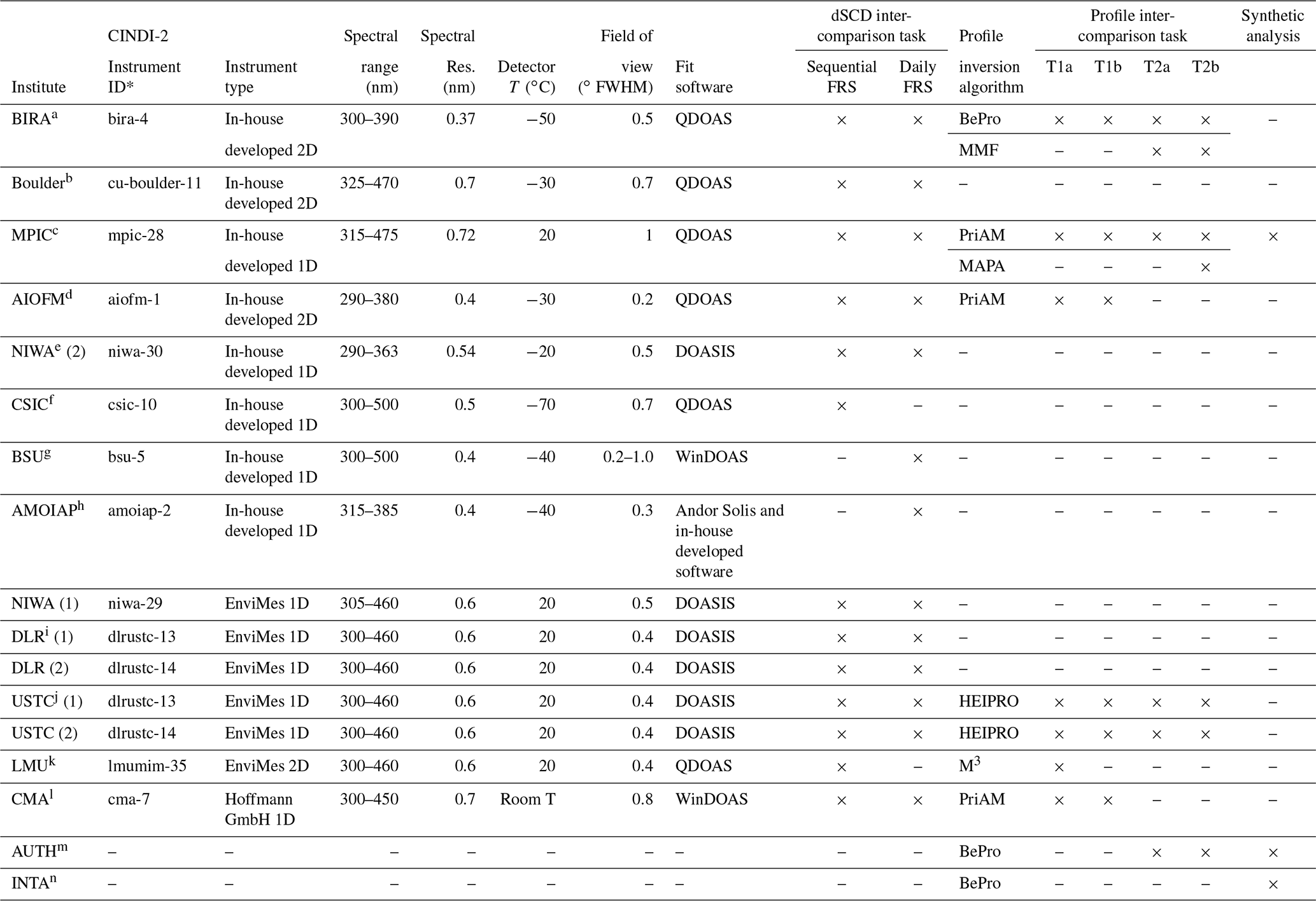
* Reference: more details of the instruments are described in Table 2 in Kreher et al. (2019). ^a Royal Belgian Institute for Space Aeronomy, Belgium. ^b Department of Chemistry and Biochemistry, University of Colorado, USA. ^c Max Planck Institute for Chemistry, Germany. ^d Anhui Institute of Optics and Fine Mechanics, Chinese Academy of Sciences, China. ^e National Institute of Water and Atmospheric Research, New Zealand. ^f Spanish National Research Council, Spain. ^g National Ozone Monitoring Research and Education Center BSU (NOMREC BSU), Belarusian State University, Belarus. ^h A. M. Obukhov Institute of Atmospheric Physics, Russia. ⁱ Deutsches Zentrum für Luft- und Raumfahrt, Germany. ^j School of Earth and Space Sciences, University of Science and Technology of China, China. ^k Meteorologisches Institut, Ludwig-Maximilians-Universität München, Germany. ^l Chinese Academy of Meteorology Science, China Meteorological Administration, China. ^m Laboratory of Atmospheric Physics, Aristotle University of Thessaloniki, Greece. ⁿ National Institute of Aerospatial Technology, Spain.

2.2 Inter-comparison of tropospheric HONO slant column densities

2.2.1 Baseline retrieval settings and comparison schemes

Baseline DOAS retrieval settings were selected based on the recommended settings from a previous study during the MAD-CAT campaign (Wang et al., 2017c). The parameters of the baseline settings are given in Table 2. Different participants applied the baseline settings using different DOAS fit programs independent of each other. Absorption cross sections of HONO, NO₂, O₃, BrO, O₄, HCHO, and H₂O were convolved with the slit function of the individual instruments before being included in DOAS fits. The slant column density (SCD) represents the trace gas concentration integrated along the light path. Differential SCDs (dSCDs) are the direct output from a DOAS fit of a measured spectrum and represent the difference of the SCDs in a measured spectrum and a Fraunhofer reference spectrum. The Fraunhofer reference spectrum is usually measured at the elevation angle of 90^∘ in order to acquire the shortest light path in the troposphere. If both the measured off-zenith spectrum and the Fraunhofer reference spectrum in a DOAS fit are recorded at approximately the same solar zenith angle (SZA), the retrieved dSCD only contains the absorptions along the light path in the troposphere, since both measurements have almost the same stratospheric light path. Therefore, in such cases, the retrieved dSCD directly represents the tropospheric SCD. In the pioneering study of Hönninger et al. (2004), it is referred to as delta SCD. Since delta SCDs are normally used in the retrievals of tropospheric vertical profiles, we first inter-compare the HONO delta SCDs between the different instruments. There are two procedures to retrieve delta SCDs from off-zenith MAX-DOAS measurements, which use two different Fraunhofer reference spectra (FRS), namely the so-called “sequential FRS” and “daily noon FRS”. The “sequential FRS” is derived from interpolation of two spectra measured in zenith view before and after an elevation sequence to match the time of the off-zenith measurements. The “daily noon FRS” is obtained from the mean of all zenith-sky spectra acquired between 11:30:00 and 11:41:00 UTC on individual days. The differential SCDs retrieved using the “sequential FRS” can directly be regarded as the delta SCDs. In contrast, a post-processing is needed to convert the differential SCDs (dSCDs) retrieved using the “daily noon FRS” into delta SCDs. For individual HONO dSCDs retrieved from off-zenith measurements, a reference dSCD can be derived by a time interpolation of the HONO dSCDs retrieved from zenith measurements before and after the off-zenith measurement. The HONO delta SCDs is then derived by subtracting this reference dSCD from the corresponding off-zenith dSCDs. The mathematical derivation of delta dSCDs with the two procedures has been discussed in Sect. 3.1 of Wang et al. (2017c). Although the “sequential” FRS can compensate for the effects of instability of instrumental properties on DOAS retrievals, the “daily noon FRS” is easier to implement in typical DOAS programs than the “sequential FRS”. Therefore the “daily noon FRS” was often used in previous studies. In this study, comparison activities of HONO delta SCDs are separated into two parts: for retrievals using either the “sequential FRS” or the “daily noon FRS”, the results of the different instruments are compared. Additionally, for individual instruments, the HONO delta SCDs retrieved using the two different FRS are also compared in order to quantify the potential bias of the HONO retrievals due to the different FRS procedures.

Table 2 Baseline DOAS analysis settings for the HONO fit.

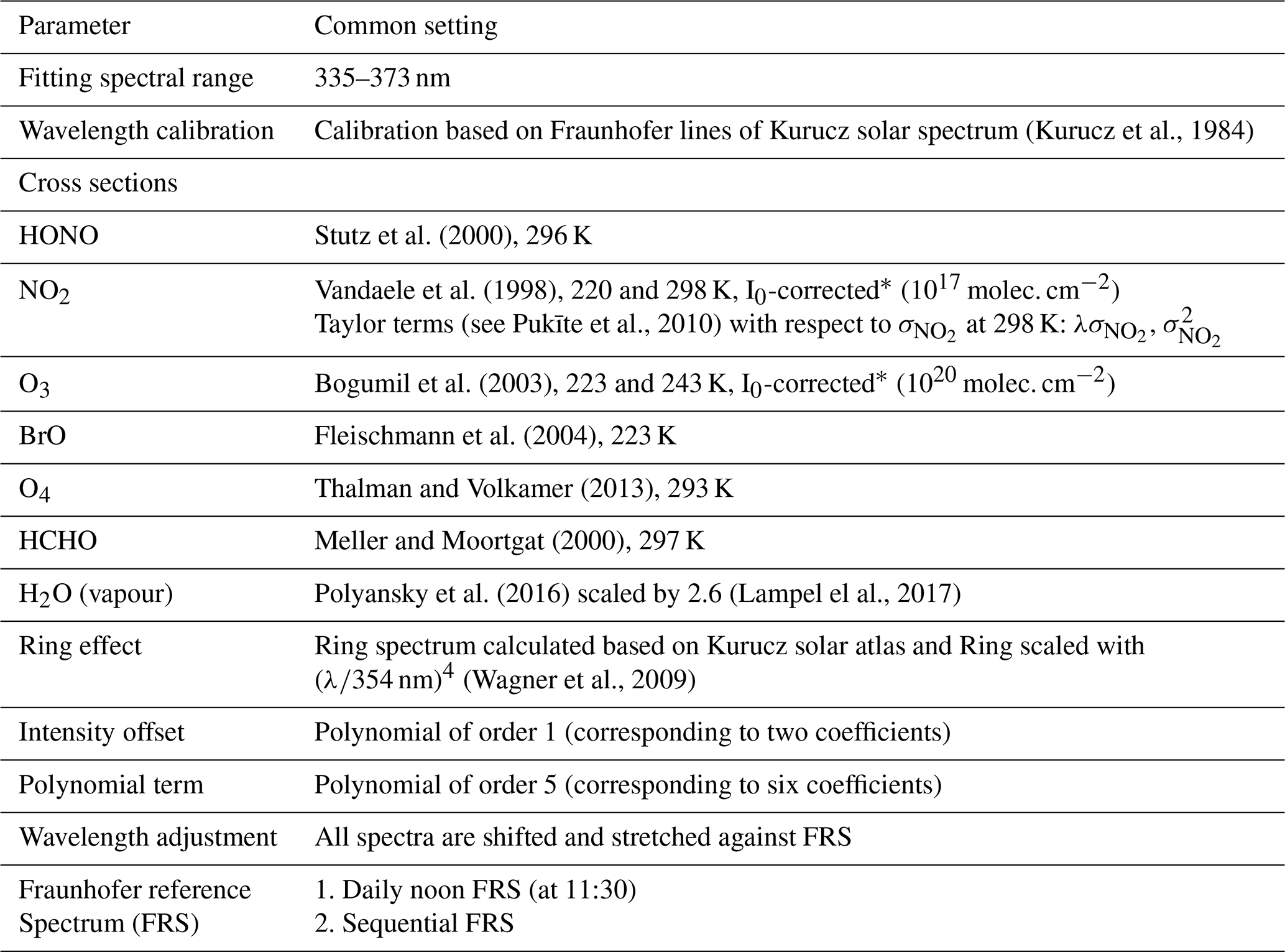
* Solar I₀ correction, Aliwell et al. (2002).

2.2.2 Participating instruments

The institutes and instruments participating in the SCD inter-comparison activities are listed in Table 1. It should be noted that “USTC (1)” and “USTC (2)” represent two data sets derived from two MAX-DOAS instruments operated by the “USTC” researchers. Additionally, the spectra recorded by the two “USTC” instruments are independently analysed by the “DLR” researchers, which are marked as “DLR (1)” and “DLR (2)”. Considering the different measurement protocols followed by the 2D system and 1D system instruments, only coincident measurements in the first 15 min of each hour are included in the inter-comparison activities. The participating instruments are separated into three groups, consisting of in-house developed instruments by individual groups, EnviMes instruments developed at the University of Heidelberg (Lampel et al., 2015) and recently commercialized (http://www.airyx.de, last access: 20 September 2020), and Mini-DOAS instruments produced in Germany by Hoffmann GmbH (http://www.hmm.de/, last access: 20 September 2020).

2.3 Inter-comparisons of tropospheric HONO profiles

2.3.1 Baseline retrieval settings and inversion algorithms

HONO profiles are retrieved from the elevation angle dependency of the HONO delta SCDs using inversion algorithms. Five inversion algorithms based on the optimal estimation (OE) method are used in this study: PriAM (Y. Wang et al., 2013a, b, 2017b), BePro (Clémer et al., 2010), MMF (Friedrich et al., 2019), HEIPRO (Frieß et al., 2006, 2011), and M³ (Chan et al., 2018). Different from the other algorithms, MAPA (Beirle et al., 2019) implemented by the “MPIC” participants is based on a profile parameterization. The corresponding algorithms implemented by individual participants are listed in Table 1. Note that PriAM, BePro, and HEIPRO are independently implemented by several participants. Some parameters are harmonized between the different inversion algorithms. Information on these parameters and on the atmospheric properties used in the RTM is summarized in Table 3. Note that no assumptions about the measurement uncertainty covariance, a priori profiles, and a priori covariance matrices are made in MAPA. The wavelength of the RTM simulations of the HONO AMFs for the profile retrievals is 355 nm, representing the effective wavelength of the HONO absorption in the spectral range of DOAS fits of HONO delta SCDs. The effective wavelength is calculated by weighting the wavelengths by the HONO cross-section values in the spectral range of 335–373 nm of the HONO DOAS fits. The atmospheric properties and aerosol properties are set based on typical conditions near the measurement site during the CINDI-2 campaign period. Profiles are retrieved in the altitude range of 0 to 4 km with a grid of 200 m. Vertical profiles of aerosol extinction are required as an input for the HONO profile retrievals and were retrieved around 360 nm from O₄ delta SCDs, which are retrieved from the MAX-DOAS measurements in the spectral range of 338–370 nm. The details of the aerosol retrievals can be found in Tirpitz et al. (2020). Following previous studies (e.g. Hendrick et al., 2014; Wang et al., 2018), the covariance of the measurement uncertainties is set to a square of 100 % of the DOAS fit error of the HONO dSCDs for the diagonal elements and zero for the extra-diagonal elements. The a priori profile is arbitrarily set as an exponentially decreasing profile with a vertical column density (VCD) of 3×10¹⁴ molec. cm⁻² and a scaling height (SH) of 0.1 km. The selection of the a priori profile shape is based on the fact that HONO is typically accumulated at altitudes close to the surface (Hendrick et al., 2014; Wang et al., 2018). Similar to measurement uncertainties, and following the previous studies (e.g. Hendrick et al., 2014; Wang et al., 2018), the covariance of the a priori profile (S_a) is set to a square of 100 % of a priori values for the diagonal elements. The extra-diagonal elements are calculated using a Gaussian function based on the neighbouring diagonal elements with a correlation length of 200 m.

Table 3 Common settings of the HONO profile retrievals.

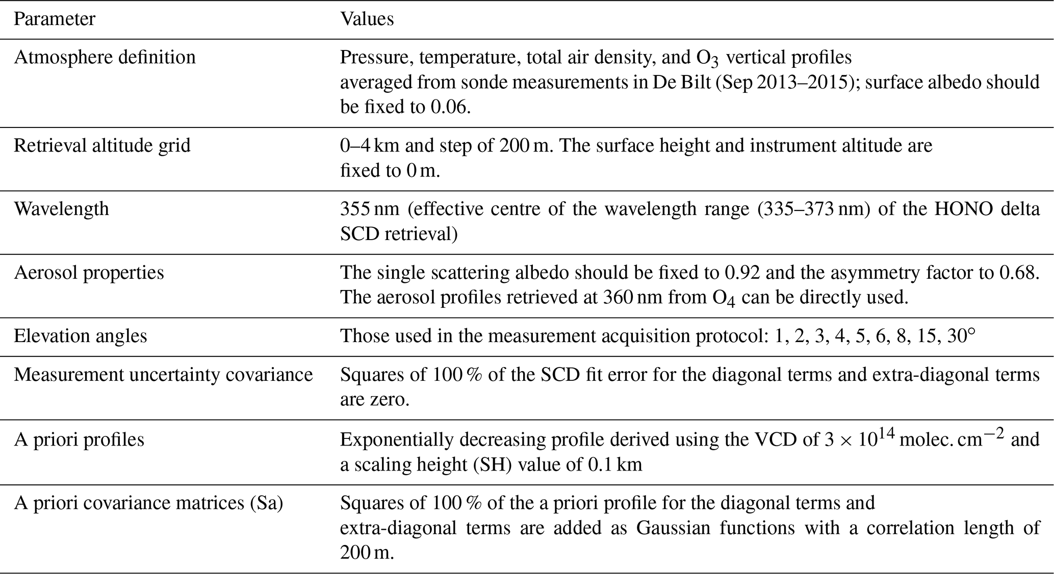
For the algorithms based on the optimal estimation method, each of them used different RTMs as the forward model and applied different iterative procedures. PriAM and HEIPRO use the RTM SCIATRAN, version 2 (Rozanov et al., 2005). BePro, MMF, and M³ use the RTMs LIDORT (Spurr et al., 2008), VLIDORT (Spurr et al., 2013), and LibRadTran (Mayer and Kylling, 2005; Emde et al., 2016), respectively. Another important difference is that in order to avoid negative concentrations of the retrieved results (which are not possible in the real atmosphere), the retrievals are done in logarithmic space (see details in Yilmaz, 2012) by PriAM, HEIPRO, and MMF. Since distribution probabilities of retrieved profiles around a priori profiles become asymmetric due to the inversion in the logarithm space, the sensitivity of the inversion to large values is larger than that in the linear space. A non-linear iterative procedure is applied for the inversion of both aerosol and trace gas profiles in PriAM, HEIPRO, and MMF, whereas a linear iterative procedure is adapted for trace gas retrievals in the other two algorithms.

2.3.2 Comparison scheme

In order to attribute the discrepancies between the different data sets of HONO profiles to different possible causes (instrumental properties, FRS selection, profile inversion algorithms, and aerosol inversions), the inter-comparison of the HONO profiles is subdivided into four tasks named T1a, T1b, T2a, and T2b. In all four tasks, the HONO profiles are retrieved using different inversion algorithms by individual participants, while the differences between the tasks are the choices of the input HONO delta SCDs and aerosol profiles.

In tasks T1a and T1b, the input HONO delta SCDs are those retrieved from measurements of the individual instruments by the individual participants. Differently, in tasks T2a and T2b, different participants use the same HONO delta SCDs, which are retrieved from measurements of the “MPIC” instrument by “MPIC”. Using different input delta SCDs allows investigation of whether the discrepancies of the HONO profiles are related to differences of HONO delta SCD retrievals or the profile inversion algorithms, respectively. For tasks T1a and T1b either the “sequential FRS” or the “daily noon FRS” was used in the DOAS fits, respectively, which allows us to quantify the effect of the FRS selections on the HONO profile retrievals. Tasks T2a and T2b differ with regard to the input profiles of aerosol extinction used for HONO profile inversion. In task T2a, different participants used the same aerosol profiles, which are retrieved from the O₄ delta SCDs derived from the “MPIC” MAX-DOAS measurements using the “PriAM” algorithm by “MPIC”. However, in task T2b, the input aerosols are retrieved from the O₄ delta SCDs, derived from the individual MAX-DOAS instruments by the respective participants. Using different input aerosol profiles allows quantification of the effects of aerosol retrievals on the consistency of the HONO profile retrievals. It should be noted that the input profiles of aerosol extinctions in tasks T1a, T1b, and T2b are the same and are derived from the aerosol profile retrievals at 360 nm, as given in Tirpitz et al. (2020), using the common settings by the individual participants. In addition, since different measurement protocols are followed by 2D systems and 1D systems (see Sect. 2.2.2), only the coincident HONO measurements in the first 15 min of each hour are included in the comparison activities.

2.3.3 Long-path DOAS measurements for comparisons with MAX-DOAS results

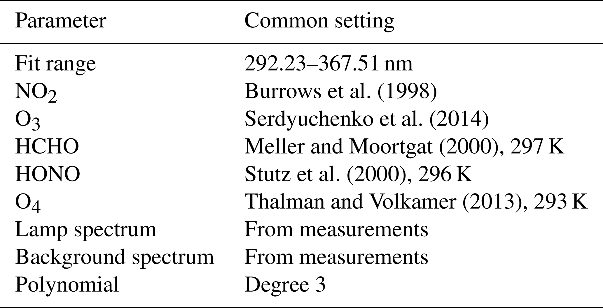
A co-located long-path (LP-)DOAS instrument measured HONO concentrations near the surface using an artificial light source during the campaign. The telescope of the LP-DOAS was installed west of the measurement site at a distance of 3800 m. A detailed description of the instrumental set-up can be found elsewhere (Nasse et al., 2019). Four retro-reflector arrays were mounted at different heights (15, 45, 105, and 205 m) at the Cabauw meteorological measurement tower close to the MAX-DOAS site. Consecutive measurements were performed on each retro-reflector, leading to a time resolution of approximately 15 min. The measurements with the retro-reflector at the height of 205 m result in average HONO concentrations along the light path, which are compared with HONO concentrations in the lowest 200 m layer of profiles derived from MAX-DOAS measurements in Sect. 4.2.2 and 4.3.3. The DOAS fit settings for the retrievals of HONO are given in Table 4.

Table 4 LP-DOAS analysis settings.

2.3.4 Synthetic dSCDs for sensitivity analysis

In most of the cases, the true HONO profiles are not known for real MAX-DOAS measurements, which makes it difficult to quantify biases of retrieved HONO profiles with respect to reality. In order to overcome this limitation, we generated a set of synthetic HONO delta SCDs using the RTM SCIATRAN, version 3.6.0 (3 December 2015) (Rozanov et al., 2014) assuming three different HONO profiles shown in Fig. 1a. The three HONO profiles represent scenarios with HONO accumulated near the surface (profile 1), linearly decreasing with altitude from the surface up to 0.8 km (profile 2), and a box-shaped profile with constant HONO VMRs in the altitude range from the surface up to 0.8 km and exponentially decreasing to zero above (profile 3). The HONO delta SCDs are simulated by the RTM at 355 nm, according to the effective wavelength of HONO DOAS fits in a pseudo-spherical atmosphere with pure Rayleigh scattering (no clouds and aerosols) and with typical temperature and pressure profiles during the campaign. HONO is the only absorber included in the simulations, and the observation geometry is set according to the real measurements on 14 September 2016, during the CINDI-2 campaign. In order to test the effect of the measurement noise, we generated a modified data set by adding artificial random noise to the HONO delta SCDs simulated by the RTM with a signal-to-noise ratio of 3000, which was determined based on the typical noise level of most of the MAX-DOAS instruments in the study. One-hundred HONO delta SCDs were generated by adding noise to the individual simulated HONO delta SCDs. This modified data set of HONO delta SCDs with artificial noise is referred to as “noisy synthetic HONO delta SCDs” in the following (see Sect. 5.1). All the synthetic HONO delta SCDs are used in the sensitivity studies presented in Sect. 5.1. The profiles shown in Fig. 1b are used as a priori profiles in the sensitivity studies.

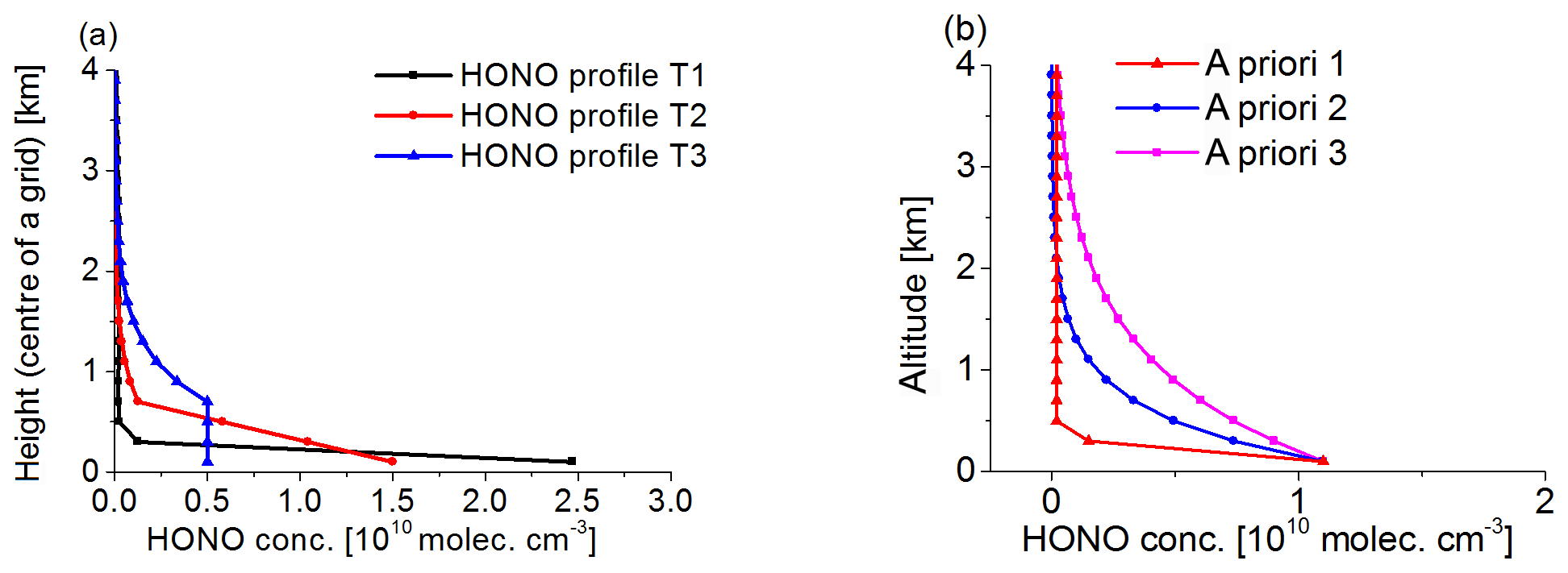
Figure 1 (a) Assumed HONO profiles used for the RTM simulations of the HONO delta SCDs. (b) Three different a priori profiles which were used for the sensitivity studies based on synthetic HONO delta SCDs.

2.4 Cloud classification

In order to evaluate the cloud effects on the MAX-DOAS results and their consistency, the cloud classification scheme described in Wang et al. (2015) and Wagner et al. (2014, 2016) was applied to the MPIC MAX-DOAS measurements during the whole CINDI-2 campaign. The sky conditions are identified from the colour index (ratio of intensities at 330 and 390 nm) and the O₄ dSCDs (retrieved in the spectral range of 338–370 nm) derived from MAX-DOAS measurements of individual elevation sequences. From the classification scheme, six categories are identified, including (a) “cloud free and low aerosol load”, (b) “cloud free and high aerosol load”, (c) “cloud holes”, (d) “broken clouds”, (e) “continuous clouds”, and (f) “optically thick clouds”. Here, the difference between categories (c) and (d) is given by the general optical thickness: it is larger for “broken clouds” than for “cloud holes”. In order to simplify the comparison activities, the categories of “cloud free and low aerosol load” and “cloud free and high aerosol load” are combined and treated as “clear sky” in this study. The remaining categories, except “optically thick clouds”, are treated as “cloudy sky”. It should be noted that the results for the category “optically thick clouds” are not included in the comparisons because the HONO retrieval quantity is usually strongly degraded for such conditions (Wang et al., 2017b).

3 Results of inter-comparison of tropospheric HONO dSCDs

In this section we present the inter-comparison of HONO delta SCDs derived by the individual participants from their MAX-DOAS measurements using the baseline settings of the DOAS fits (see Sect. 2.2). The overview of the results of the HONO delta SCDs is presented in Sect. 3.1. The overall statistics of the inter-comparisons and the comparison results for the individual participants are discussed in Sect. 3.1 and 3.2, respectively.

3.1 Overview of tropospheric HONO delta SCDs during the CINDI-2 campaign

For the comparison of the HONO delta SCDs, median values are calculated from the HONO delta SCDs derived from all participants for individual elevation angles separately for the HONO delta SCDs retrieved using the “sequential FRS” and the “daily noon FRS”, respectively. The time series of median delta SCDs using the “sequential FRS” are shown in the top panel of Fig. 2a for the time interval of 06:00 to 17:00 UTC on the individual days of the campaign. The corresponding sky conditions identified from the MPIC MAX-DOAS measurements (see Sect. 2.4) are given in the bottom panel of Fig. 2a. The sky condition results indicate that the frequencies of the “clear-sky” and “cloudy-sky” conditions are almost equal during the whole campaign. The peak values of the HONO delta SCDs typically appear in the early morning, except 27 September, when the peak value of $\sim \mathrm{3}\times {\mathrm{10}}^{\mathrm{15}}$ molec. cm⁻² is found between 08:00 and 10:00 UTC. The peak values in the early morning reach values up to $\sim \mathrm{8}\times {\mathrm{10}}^{\mathrm{15}}$ molec. cm⁻², as e.g. observed on 21 and 22 September. A large spread of HONO delta SCDs along the elevation angles can be seen and usually with maximum values typically at a 1^∘ elevation angle.

Figure 2 Overview of the HONO delta SCDs retrieved from all MAX-DOAS instruments using the “sequential FRS” during the whole CINDI-2 campaign period. (a) Time series of median HONO delta SCDs derived from measurements of all MAX-DOAS instruments by individual groups. The results of the cloud classification algorithm (applied to the “MPIC” measurements) are shown at the bottom of the subfigures. The colours indicate the elevation angles and cloud categories, respectively. The colours in (b), (c), and (d) indicate elevation angles as shown in the upper panel of (a). (b) Diurnal variations of hourly median HONO delta SCDs derived from all MAX-DOAS instruments. (c) Diurnal variation of hourly standard deviations of differences from median HONO delta SCDs from all MAX-DOAS instruments. (d) Hourly median and standard deviations of the DOAS fit errors of the HONO delta SCDs from all MAX-DOAS instruments. The left, centre, and right columns of subfigures represent the results for all the data as well as results for “clear-sky” and “cloudy-sky” conditions, respectively.

3.2 Statistical inter-comparisons of HONO delta SCDs

For the results using the “sequential FRS”, median diurnal variations for individual elevation angles of all data sets from all participants are calculated and shown in Fig. 2b. Note that the median values are calculated over both measurement time and all instruments. HONO delta SCDs strongly decrease with increasing elevation angles, especially in the morning, and the spread of the HONO delta SCDs along elevation angles decreases steeply during the day. At 06:00 UTC the HONO delta SCDs are $\sim \mathrm{3.2}\times {\mathrm{10}}^{\mathrm{15}}$ molec. cm⁻² and $\sim \mathrm{0.2}\times {\mathrm{10}}^{\mathrm{15}}$ molec. cm⁻² for elevation angles of 1 and 30^∘, respectively. During the day, a continuous decrease in the HONO delta SCDs for elevation angles of 1^∘ is seen, with the strongest decrease from $\sim \mathrm{3.2}\times {\mathrm{10}}^{\mathrm{15}}$ to $\sim \mathrm{1.2}\times {\mathrm{10}}^{\mathrm{15}}$ molec. cm⁻² between 06:00 and 08:00 UTC. For the high elevation angles, the change is much smaller. For instance, the HONO delta SCDs are $\sim \mathrm{0.2}\times {\mathrm{10}}^{\mathrm{15}}$ molec. cm⁻² at the elevation angles of 30^∘ during the whole day.

In order to evaluate the agreement of the HONO delta SCDs between the different participants, for the same data sets, the diurnal variation of the standard deviation of all HONO delta SCDs compared to the median values as shown in Fig. 2a is calculated and shown in Fig. 2c. Note that temporal variations of HONO delta SCDs do not impact the standard deviations because the median values in the individual time steps shown in Fig. 2a served as a reference in the calculations. The standard deviation is much larger in the early morning ($\sim \mathrm{1.2}\times {\mathrm{10}}^{\mathrm{15}}$ molec. cm⁻²) at 06:00 UTC than those at a later time. The standard deviations are slightly larger at low elevation angles than those at high elevation angles. Compared to the median values of the HONO delta SCDs, the relative standard deviation is much smaller at low elevation angles (e.g. 40 %–100 % at 1^∘ elevation angle) than at high elevation angles (e.g. 200 %–400 % at 30^∘ elevation angle). Similarly, the relative standard deviation in the afternoon is much larger than that in the early morning, e.g. 40 % at 06:00 UTC and 100 % at 15:00 UTC, consistent with lower daytime HONO concentrations (and thus larger relative measurement errors) at the measurement site. Since the DOAS fit errors indicate the uncertainties of the DOAS retrieval of the HONO delta SCDs, the diurnal variation of the median and standard deviation of the fit errors of all the data sets is also shown in Fig. 2d. As demonstrated for other trace gas species in Kreher et al. (2019), the DOAS fit errors and standard deviations of HONO delta SCDs should be comparable under ideal conditions, which means different instruments measuring with exactly the same field of view (FOV) and acquisition time under stable atmospheric conditions. However, those ideal conditions can not be perfectly reached in reality. By comparing Fig. 2c and d, one can see that the fit errors are smaller than the standard deviation of the HONO delta SCDs by $\sim \mathrm{0.3}\times {\mathrm{10}}^{\mathrm{15}}$ molec. cm⁻², i.e. by about 50 %. This feature indicates that the effects of atmospheric variability in the FOV of ∼1^∘ (corresponding to a round sky area with a radius of ∼100 m under a frequent maximum visible distance of ∼10 km) and discrepancies of FOV and acquisition time between the different instruments can considerably contribute to random discrepancies of HONO delta SCD measurements. A similar conclusion was obtained in the previous studies of Kreher et al. (2019) and Bösch et al. (2018). The differences of random discrepancies and DOAS fit errors depend on actual instrumental noise levels, measured species, and atmospheric variability conditions. Regarding the dependence on measured species, Kreher et al. (2019) reported that random discrepancies of NO₂ dSCDs in the visible range are larger than DOAS fit errors by an order of magnitude. Comparisons of DOAS fit errors and random discrepancies of HONO delta SCDs will be discussed for individual instruments in Sect. 3.3.1.

In order to evaluate the effect of clouds on the consistency of the HONO delta SCDs between the different data sets, we show the diurnal variation of the median values of the HONO delta SCDs, corresponding standard deviations, and the median and standard deviations of the DOAS fit errors separately calculated for measurements under “clear-sky” and “cloudy-sky” conditions (see Sect. 2.4 about the cloud classification) in Fig. 2. In general, similar values of all the quantities are found for both sky conditions, probably due to the fact that HONO abundances are mostly near ground level and HONO absorption light paths are not considerably affected by clouds located at high altitudes. However, for the standard deviation of the HONO delta SCDs, larger values are found under “cloudy-sky” conditions than under “clear-sky” conditions. The standard deviation of the DOAS fit error under “cloudy-sky” conditions is larger than under “clear-sky” conditions. This finding might be attributed to two factors: (1) the rapid variation of cloud properties for conditions of inhomogeneous cloud coverage; (2) the enhanced photon shot noise, due to the fact that fewer photons are received by instruments under “cloudy-sky” conditions, can result in larger random noise and further larger discrepancies of HONO delta SCDs between different instruments compared to those under “clear-sky” conditions. Wagner et al. (2014) demonstrated that the number of photons (proportional to measured radiance) is typically reduced by more than 10 % under optically thick clouds compared to those under clear-sky conditions. In addition, results similar to that shown in Fig. 2 are also observed for the data sets retrieved using the “daily noon FRS”. Hence, we only show the results of using the “sequential FRS”.

3.3 Comparison results for individual participants

For the data sets of HONO delta SCDs from individual participants, linear regressions against the median values are calculated for the whole campaign. The corresponding correlation coefficients, slopes, intercepts, and root mean square (rms) of the residuals are shown in Fig. 3a, b, c, and d, respectively. The corresponding median values and standard deviations are presented in Fig. 3e. The median values and standard deviations of the DOAS fit error are shown in Fig. 3f. For the intercepts, rms, median differences, and fit errors shown in Fig. 3d, e, and f, a second y scale is added on the right-hand side of the diagrams. It indicates the typical relative discrepancy compared to a typical high value of the HONO delta SCDs of 2×10¹⁵ molec. cm⁻². This quantity is referred to as the “typical percentage” in the subsequent part of this section. Since the HONO profile retrievals are dominated by measurements at low elevation angles, the comparison results for 1^∘ elevation are separately plotted in Fig. 3 (red and green dots). Also, the comparison results for analyses using a “sequential FRS” or “daily noon FRS” are individually presented.

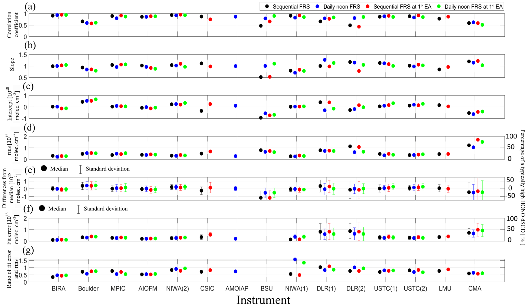
Figure 3 Correlation coefficients (a), slopes (b), intercepts (c), and rms of the residuals (d) derived from the linear regressions versus the median values. The median differences and standard deviations derived from the comparison of the HONO delta SCDs from individual instruments and the median values of all instruments during the whole CINDI-2 campaign period are shown in (e). In (f) the median values and the standard deviation of the DOAS fit error are shown. The y axis on the right-hand side of (d), (e), and (f) indicates percentages calculated by dividing the absolute errors by a typical high HONO delta SCD of 2×10¹⁵ molec. cm⁻². In (g) ratios of rms and DOAS fit errors are shown.

The discrepancies of the HONO delta SCDs between the different MAX-DOAS instruments consist of random and systematic discrepancies. The random discrepancies can be minimized by averaging over a large number of measurements since instrumental noise and spatial–temporal variations of sky conditions and pollutants can be smoothed out by the averaging. The effect has been studied in Peters et al. (2019). In Fig. 3d, the rms values of residuals of linear regressions against the median values can represent the random measurement errors similarly to the standard deviations of HONO delta SCDs discussed in Sect. 3.2, whereas the slopes, intercepts, and median differences shown in Fig. 3b, c, and e indicate the systematic discrepancies. For comparisons with the rms values, the DOAS fit errors from individual participants are also shown in Fig. 3f.

3.3.1 Random discrepancies

The rms values shown in Fig. 3d for HONO delta SCDs are lower than $\sim \mathrm{0.6}\times {\mathrm{10}}^{\mathrm{15}}$ molec. cm⁻² for most of the participants, corresponding to a “typical percentage” of 30 %. The rms values obtained using a “sequential” FRS and a “daily noon FRS” are similar in magnitude for most of the participants if all elevation angles or only the 1^∘ elevation angle are considered. The lowest rms values of $\sim \mathrm{0.3}\times {\mathrm{10}}^{\mathrm{15}}$ molec. cm⁻², corresponding to a “typical percentage” of 15 %, are reached by the “BIRA”, “NIWA (2)”, “AMOIAP”, and “NIWA (1)” instruments. Even though the “NIWA (1)” instrument belongs to the group of “EnviMes” instruments, a lower rms is reached by the “NIWA (1)” instrument compared to the other “EnviMes” instruments. The improved performance might be attributed to the customized productions and personalized operation of the individual “EnviMes” instruments as well as different implementations of the DOAS fits by the individual participants. Another interesting finding for the “EnviMes” instruments is that although the same set of spectra measured by the “USTC” instruments (see Table 1) is analysed by the “DLR” and “USTC” researchers, much larger rms values and fit errors are found for the “DLR(1)” and “DLR(2)” results (especially for the “DLR(2)” results with the “sequential FRS”) than for the “USTC(1)” and “USTC(2)”. This finding implies that random discrepancies between the data sets can be considerably attributed to the specific implementation of the DOAS fits and the characteristics of the instrumental slit functions by the individual participants. The previous study of Peters et al. (2017) demonstrated that differences in DOAS retrieval codes can result in discrepancies of retrieved NO₂ dSCDs and rms residuals by up to 8 % and 100 %, respectively. Since optical depths of HONO absorptions are typically much lower than NO₂, the effect of differences in DOAS retrieval codes and DOAS implementations by individual participants on retrieved HONO dSCDs might be relatively larger than that on NO₂. The “CMA” rms values derived for a Hoffmann Mini-DOAS instrument are the largest (∼1 to 1.7×10¹⁵ molec. cm⁻², corresponding to a “typical percentage” of 30 % to 85 %). The large rms of “CMA” is consistent with its large fit error of $\sim \mathrm{1}\times {\mathrm{10}}^{\mathrm{15}}$ molec. cm⁻². Therefore, we conclude that the Hoffmann Mini-DOAS instruments can hardly reach the signal-to-noise requirements for HONO measurements in cases of HONO dSCDs lower than $\sim \mathrm{2}\times {\mathrm{10}}^{\mathrm{15}}$ molec. cm⁻².

Figure 3g shows the ratios of DOAS fit errors and the rms values for individual data sets. This relates to the discussion at the end of Sect. 3.2 on the differences of DOAS fit errors and random discrepancies. Fig. 3g indicates that the ratios are different for different data sets and in the range of 0.3 to 1.6. For most of the data sets, the ratios are lower than unity, indicating that effects of atmospheric variability and discrepancies of instrumental FOV and acquisition time dominate random discrepancies more than the effect of instrumental noise given by DOAS fit errors. The lowest ratio of 0.3 is found for the “BIRA” data set. It indicates that the dominant factors of the random discrepancies of the “BIRA” data set are atmospheric variability and instrumental discrepancies, but not instrumental noise.

3.3.2 Systematic discrepancies

For an overview of the systematic biases, median differences of the individual data sets of HONO delta SCDs from the median values are calculated and shown in Fig. 3e. These biases are mostly in the range of $\pm \mathrm{0.3}\times {\mathrm{10}}^{\mathrm{15}}$ molec. cm⁻², corresponding to a “typical percentage” of about ±15 %. The slopes derived from the linear regression mostly deviate from unity by about ±20 % and the intercepts are mostly in the range of $\pm \mathrm{0.3}\times {\mathrm{10}}^{\mathrm{15}}$ molec. cm⁻², which corresponds to a “typical percentage” of about ±15 %. For the individual data sets, the median differences are generally consistent with the intercepts but not the slopes. This finding is related to the fact that low and high HONO delta SCDs dominate the intercept and slope derived from the linear regression. Since low values are more frequent than large values, the median values of the differences are dominated by the lower HONO delta SCDs. Hence the intercepts and slopes mainly represent the systematic discrepancies of low and high values of the HONO delta SCDs, respectively, whereas the median differences indicate the general bias. For the data sets from “BIRA”,”MPIC”, “AIOFM”, “NIWA (2)”, “AMOIAP”, “USTC (1)”, “USTC (2)”, and “LMU”, the median differences, slopes, and intercepts are all in the range of $\pm \mathrm{0.3}\times {\mathrm{10}}^{\mathrm{15}}$ molec. cm⁻², ±20 % deviation from unity, and $\pm \mathrm{0.3}\times {\mathrm{10}}^{\mathrm{15}}$ molec. cm⁻², respectively, representing the corresponding typical ranges. Much larger biases of the slopes (∼0.5) are found for the “BSU” data with “sequential FRS” than that for those with “daily noon FRS”. The reason for this finding is not yet identified. For the “DLR (1)” and “DLR (2)” data, although the median differences fall within the range of typical values, different biases (about plus 30 % or minus 30 % for large HONO delta SCDs, as indicated by the slopes) are found for “DLR (1)” with “daily noon FRS” and the “DLR (2)” with the “sequential FRS” at 1^∘ elevation angle, respectively. Considering that the “DLR” data are derived from the same set of spectra as the “USTC” data, the different implementations of the DOAS fits by both participants might have caused the different results. For the “CMA” data sets, although the deviations of the slopes from unity are within about 20 %, the median differences and intercepts of about $-\mathrm{0.5}\times {\mathrm{10}}^{\mathrm{15}}$ molec. cm⁻² indicate a larger underestimation of low HONO delta SCDs than for the other participants. However, here it should be noted that the correlation coefficient is also rather low (r∼0.6).

In order to further characterize the diurnal variation of the discrepancies for the individual participants, the median and 25th and 75th percentiles of the differences of the HONO delta SCDs from the medians for elevation angles of 1^∘, 5^∘, and 15^∘, respectively, are shown in Fig. 4. The comparison results for the data sets with “sequential FRS” and “daily noon FRS” are shown in subpanels a and b. Considerable diurnal variations of the discrepancies are found for the “DLR”, “BSU”, and “CMA” data. For “DLR” data, negative and positive biases usually occur in the early morning and around noon, respectively, especially if a “sequential FRS” is used. Larger negative biases in the morning and in the afternoon are observed for “CMA”. Larger negative biases of the “BSU” data with “sequential FRS” appear in the morning, whereas the “BSU” data with “daily noon FRS” show larger negative biases around noon. Additionally, different biases for different elevation angles are found for some data. For instance, the discrepancies of the “AIOFM”, “NIWA (2)”, and “USTC (2)” data are larger for the 1^∘ elevation angle than for other elevation angles in the early morning.

Figure 4 Boxplots (including median, percentiles, and extreme data) of the differences of the HONO delta SCDs for individual instruments (one instrument each row) with respect to the median values for the results using a “sequential FRS” (a) or a “daily noon FRS” (b). In the (c) column of subplots, the differences of the HONO delta SCDs for the results using a “sequential FRS” or “daily noon FRS” are shown for the individual instruments. Colours indicate the elevation angles. The gaps between the subplots are due to unavailability of the corresponding data.

In order to evaluate the effects of the FRS selection on the HONO delta SCDs, the median and percentiles of the differences of the HONO delta SCDs of both procedures are shown in Fig. 4c. The statistics of the differences are provided for different hours of the day and elevation angles of 1^∘, 5^∘, and 15^∘, respectively. For most of the data sets, including “BIRA”, “MPIC”, “Boulder”, “AIOFM”, “NIWA (2)”, “NIWA(1)”, “USTC (1)”, and “USTC (2)”, the median values of the differences are usually in the range of $\pm \mathrm{0.1}\times {\mathrm{10}}^{\mathrm{15}}$ molec. cm⁻² (corresponding to a “typical percentage” of 5 %), while the 25th and 75th percentiles are in the range of 0.2×10¹⁵ molec. cm⁻² (corresponding to a “typical percentage” of 10 %). For the “BSU” data, a large positive bias of $\sim \mathrm{3}\times {\mathrm{10}}^{\mathrm{15}}$ molec. cm⁻² is found in the early morning and decreases afterwards. The reason for this finding is not yet identified. The median differences for both “DLR” data sets are in the range of $\pm \mathrm{1.6}\times {\mathrm{10}}^{\mathrm{15}}$ molec. cm⁻² (corresponding to a “typical percentage” of $\sim \pm \mathrm{80}$ %), depending on the time of a day, whereas the differences of the 25th and 75th percentiles are about 1×10¹⁵ molec. cm⁻². However, considering the fact that both the “DLR” and “USTC” data sets are derived from the same spectra, we conclude that the different effects of the FRS selection arise from the specific implementations of DOAS fits. For the “CMA” data, the median differences are in the range of 0.2 to $-\mathrm{0.4}\times {\mathrm{10}}^{\mathrm{15}}$ molec. cm⁻². This finding probably reflects the effects of instrumental instability.

In general, for most of the instruments with moderate performance during this campaign, systematic discrepancies between the data sets are in the range of $\pm \mathrm{0.3}\times {\mathrm{10}}^{\mathrm{15}}$ molec. cm⁻², which is about half of the general random discrepancy of $\sim \pm \mathrm{0.6}\times {\mathrm{10}}^{\mathrm{15}}$ molec. cm⁻². For a typical high HONO delta SCD of 2×10¹⁵ molec.,cm⁻², the typical relative systematic and random discrepancies are about 15 % and 30 %, respectively. The lowest random discrepancy of $\sim \mathrm{0.3}\times {\mathrm{10}}^{\mathrm{15}}$ molec. cm⁻², which is comparable to the general systematic bias, can be reached by some instruments. For some data sets, the systematic differences are higher (up to $\pm \mathrm{0.5}\times {\mathrm{10}}^{\mathrm{15}}$ molec. cm⁻²), probably due to an inappropriate implementation of the DOAS fit. For most instruments, the FRS selection is not critical, as the systematic differences between the HONO delta SCDs retrieved using the “sequential FRS” or “daily noon FRS” are typically in the range of $\pm \mathrm{0.1}\times {\mathrm{10}}^{\mathrm{15}}$ molec. cm⁻².

3.3.3 Discussion on effects of misalignments of elevation angles

Misalignments of elevation angles for individual instruments might result in discrepancies of HONO delta SCDs between the instruments. Since elevation misalignments might consist of systematic offsets and temporal changes for individual instruments, the resulting discrepancies in HONO delta SCDs might be both systematic and random. We estimated the typical bias of HONO delta SCDs according to a typical misalignment of elevation angles during the CINDI-2 campaign. Donner et al. (2019) characterized biases of elevation angles as mostly smaller than 0.4^∘ for most of the MAX-DOAS instruments during the CINDI-2 campaign, based on scanning horizon and active light calibration methods applied to individual instruments. Figure 2b indicates that the largest change in HONO delta SCDs per elevation angle degree appears at the lowest elevation angles of 1^∘ to 3^∘. Therefore, effects of misalignments of elevation angles on measured HONO delta SCDs are stronger at smaller elevation angles than at larger ones. Based on the typical dependence of HONO delta SCDs on elevation angles, the biases of HONO delta SCDs at 1^∘ due to a typical elevation angle bias of 0.4^∘ can be roughly estimated as $\sim \mathrm{0.2}\times {\mathrm{10}}^{\mathrm{15}}$ molec. cm⁻² in the morning and $\sim \mathrm{0.04}\times {\mathrm{10}}^{\mathrm{15}}$ molec. cm⁻² around noon, which are only a third of typical DOAS fit errors shown in Fig. 2d and ∼10 % of typical random discrepancies shown in Fig. 2b. Furthermore, we do not observe correlation between the bias of HONO delta SCDs from the median values and identified misalignments of elevation angles for some instruments, for which considerable elevation misalignments occurred during the campaign. Overall, the misalignments of elevation angles result in negligible discrepancies of HONO delta SCDs between the instruments.

4 Inter-comparison of tropospheric HONO vertical profiles

In this section we present the inter-comparison of vertical profiles of the HONO VMRs retrieved by the different participants with different inversion algorithms for the baseline retrieval settings (see Sect. 2.3.1). An overview of the retrieved profiles is presented in Sect. 4.1. The overall statistics and comparison results for the individual participants are given in Sect. 4.2 and 4.3, respectively.

4.1 Overview of retrieved HONO profiles

Time series of the HONO profiles retrieved by the different participants between 06:00 and 17:00 UTC on individual days during the whole campaign are plotted in Fig. 5. This also includes all the profile results for the four comparison tasks described in Sect. 2.3.2. Although the HONO profiles were retrieved in the altitude range below 4 km, only the results below 1 km are shown, because above 1 km only very small HONO mixing ratios are retrieved. However, for the calculation and inter-comparison of the HONO VCDs (Sect. 4.2 and 4.3), the HONO profiles are integrated for the altitude range from 0 to 4 km. For the individual comparison tasks, the median values of the HONO profiles are calculated and also plotted in Fig. 5. All data sets indicate that HONO usually accumulates near the surface. However, considerable discrepancies in the absolute values and diurnal variations can also be seen. The sky conditions identified from the MPIC MAX-DOAS measurements (see Sect. 2.4) are shown in the bottom panel of Fig. 5. The gaps of results in Fig. 5 are due to the unavailability of data as the corresponding MAX-DOAS instruments were not operational or the profile inversion failed. For task T2b, the “MPIC (MAPA valid)” data show many more gaps than the “MPIC (MAPA)” data since the quality flag criteria (Beirle et al., 2019) were applied to the “MPIC (MAPA valid)” data. For tasks T1a and T1b, two versions of “BIRA” profile results are displayed and marked as “BIRA (v1)” and “BIRA (v2)” and discussed in Sect. 5.3. Since the “BIRA (v2)” data set is retrieved with more realistic measurement uncertainties than “BIRA (v1)”, it has been decided to only use the “BIRA (v2)” data set in the further inter-comparison analysis in Sect. 4.2 and 4.3.

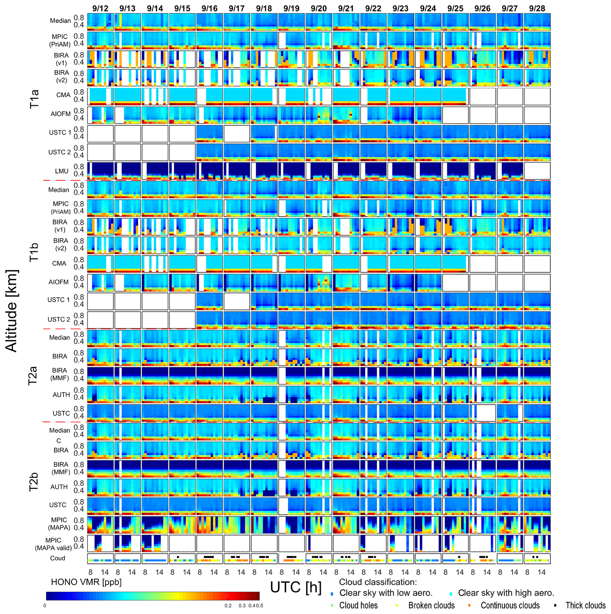
Figure 5 Overview of the time series of HONO profiles derived by different institutes and instruments for the four tasks. The median values for the individual tasks are also given. The colour map is given in logarithmic scale in order to show fine structures of low HONO VMR values above the surface. Note that the colour map starts from zero. Negative values can appear in some data sets but are generally insignificant since their mean values are about −0.007 ppb. The cloud classification results are shown in the small subfigures at the bottom.

4.2 Statistical inter-comparisons of HONO profiles, VCDs, and near-surface VMRs

4.2.1 Comparisons with median values

The diurnal variations of the median values of the HONO VCDs and near-surface VMRs for all the data sets are calculated for the individual tasks and plotted in Fig. 6a and b, respectively. A steep decrease in the HONO VCDs and near-surface VMRs from ∼3 to $\sim \mathrm{1.5}\times {\mathrm{10}}^{\mathrm{14}}$ molec. cm⁻² and from ∼0.4 to ∼0.1 ppb between 06:00 and 08:00 UTC is found, respectively. Afterwards, the VCDs and VMRs close to the surface stay at low values, with a slight decrease until 16:00 UTC. Considering the significant decrease in HONO in the early morning, the median values of the HONO profiles before and after 07:00 UTC are separately shown in Fig. 6d and e, respectively. Both figures indicate that the HONO VMRs above 0.6 km are close to zero. In addition, Fig. 6a and b indicate considerable differences in the median values of the different tasks, especially in the early morning before 08:00 UTC. These differences can primarily be attributed to differences in the input HONO delta SCDs and aerosol profiles used in the profile retrievals.

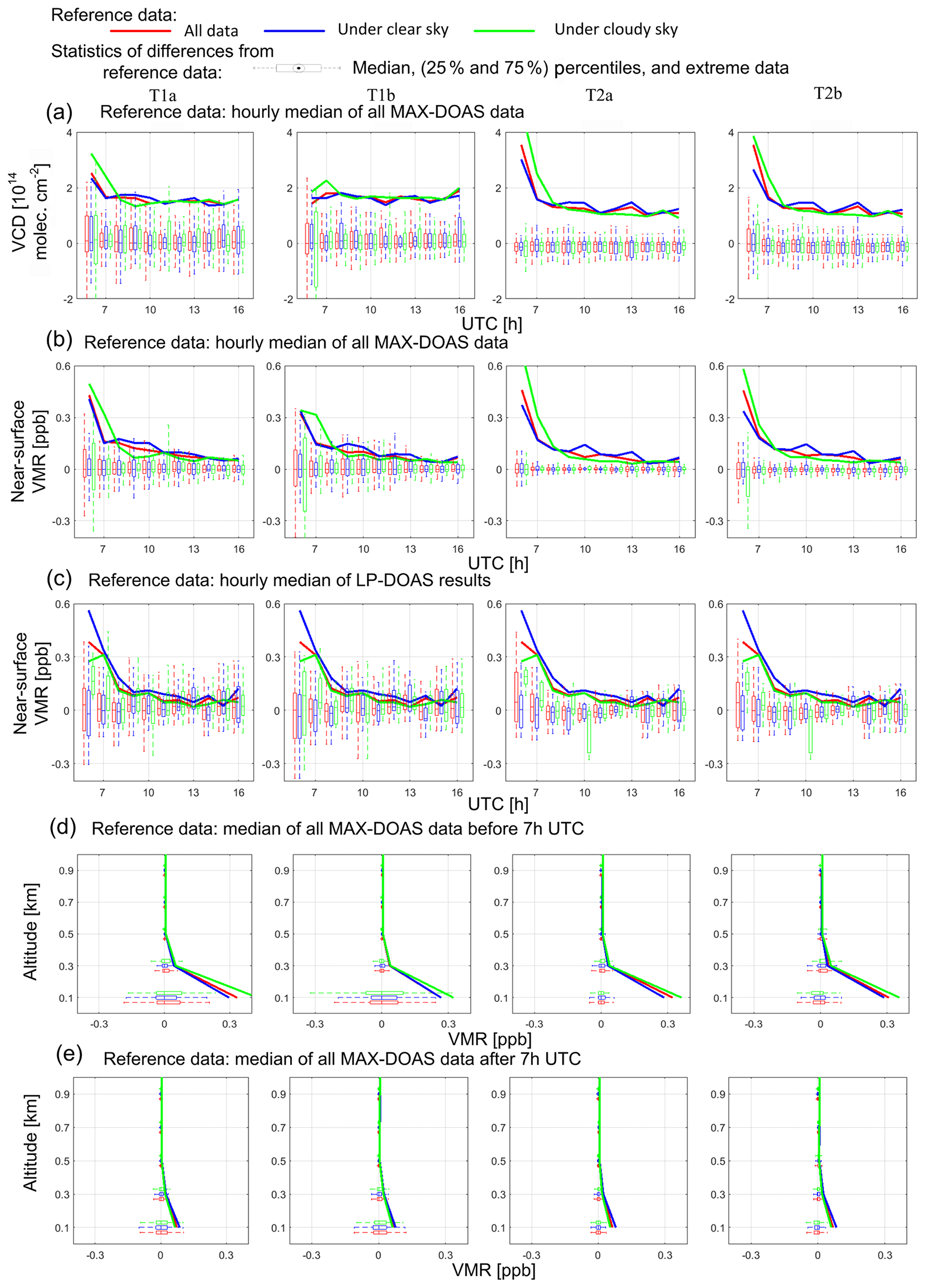
Figure 6 Boxplots of the differences of the HONO VCDs (a), near-surface VMRs (b), and profiles before (d) and after 07:00 UTC (e) derived by different institutes compared to the median values for the whole campaign. Boxplots of the differences of the HONO near-surface VMRs compared to the co-located LP-DOAS measurements are shown in (c). Note that the median values which served as the reference in the calculation of the boxplots are calculated in the individual time steps, namely each hour. Therefore, temporal variations of the quantities do not contribute to the boxplots. Colours in all subfigures indicate the sky condition. Comparisons of data sets for the four tasks are shown in the different columns of subfigures. Comparison results are calculated for different hours during the day in (a), (b), and (c). The reference values for the comparisons are also given by the solid lines in each subfigure. The reference values are the hourly median of HONO VCDs (a), near-surface VMRs (b), and profiles before (d) and after 07:00 UTC (e) derived from all MAX-DOAS data and near-surface VMRs derived from the co-located LP-DOAS measurements (c), respectively.

The 25th and 75th percentiles of the differences of the HONO VCDs, near-surface VMRs, and vertical profiles before and after 07:00 UTC compared to the median values are shown in Fig. 6a, b, d, and e, respectively, with different columns indicating the four tasks. The deviations between the different data sets are much smaller if the common HONO delta SCDs (tasks T2a and T2b) are used than if the HONO delta SCDs measured by individual instruments (tasks T1a and T1b) were used. For task T2a, the half interquartile range is mostly $\sim \mathrm{5}\times {\mathrm{10}}^{\mathrm{13}}$ molec. cm⁻² (corresponding to ∼15 % to ∼30 % of the median values) for the VCDs and ∼0.02 ppb for the near-surface VMRs (∼5 % to ∼20 % of the median values). For task T1a, the half interquartile range increased by about 3 times compared to those for task T2a. Therefore, we conclude that the discrepancies of the HONO delta SCDs can contribute ∼30 % to 60 % deviations of the HONO VCDs and ∼10 % to 40 % deviations of the near-surface VMR results. The deviations are smaller than the typical relative deviations of HONO delta SCDs of 40 %–100 % at low elevation angles, which arise due to the smoothing effect of the profile inversion. For both tasks T2a and T2b, the absolute deviations are larger in the morning than in the afternoon, but the relative deviations are similar due to larger HONO values in the morning. Also, slightly larger interquartile ranges are found for task T2b than for task T2a, especially in the morning by $\sim \mathrm{3}\times {\mathrm{10}}^{\mathrm{13}}$ molec. cm⁻² and ∼0.04 ppb, respectively. This indicates that the discrepancies of the aerosol retrievals can cause discrepancies of the HONO VCDs and near-surface VMRs by ∼50 %. Similar ranges of percentiles are found for tasks T1a and T1b, indicating that the effects of using either a “sequential FRS” or “daily noon FRS” on the consistency of the HONO profile retrievals are not critical. The comparison results of HONO profiles shown in Fig. 6d and e indicate that deviations of the HONO VMRs between different data sets are negligible at altitudes above 0.4 km, where the HONO VMRs are also almost zero.

4.2.2 Comparisons with LP-DOAS

The statistical differences (the median values and 25th and 75th percentiles) of the near-surface HONO VMRs of the different data sets compared to the co-located LP-DOAS are shown in Fig. 6c. The LP-DOAS measurements and data for the comparisons are described in Sect. 2.3.3. The median differences and half interquartile ranges are mostly in the ranges of ±0.05 ppb (∼10 % to ∼50 %) and 0.1 ppb (∼20 % to ∼100 %) for the four tasks. Systematically larger interquartile ranges are found in the early morning.

4.2.3 Cloud effects on the HONO profile results

In order to evaluate effects of clouds on the consistency of the HONO profile retrieval results, all quantities in Fig. 6 are separately shown for the measurements under “clear-sky” and “cloudy-sky” conditions. In general, similar values for the upper and lower quartiles are found for both clear- and cloudy-sky conditions, except for tasks T1a and T1b. The interquartile ranges under “cloudy-sky” conditions are ∼10 % larger than those under “clear-sky” conditions for tasks T1a and T1b, which is probably related to the larger random discrepancies of the HONO delta SCDs measured by different instruments (see Fig. 2c and Sect. 3.2).

4.3 Comparison results for individual participants

For the HONO near-surface VMRs and VCDs derived from the profile retrievals of the individual participants, linear regressions against the median values are performed. The derived correlation coefficients, slopes, intercepts, as well as rms of the residuals are shown in Fig. 7a and c. The median values and standard deviations of the differences of the individual data sets from the median values are also presented in Fig. 7a and c, and for the vertical profiles in the three altitude intervals of 0 to 0.2 km, 0.2 to 0.4 km, and 0.4 to 4 km, in Fig. 8. For the intercepts, rms, and median differences shown in Fig. 7, the corresponding “typical percentages” (relative differences compared to a typical large HONO near-surface VMR of 0.4 ppb and VCD of 3×10¹⁴ molec. cm⁻²) are also shown (see the y axis on the right-hand side). Additionally, for the comparison results of the near-surface HONO VMRs versus the LP-DOAS measurements, the same parameters as shown in Fig. 7a and c are given in Fig. 7b. The same parameters as shown in Fig. 7a and c are derived from the comparisons of the modelled and measured HONO delta SCDs and shown in Fig. 7d. It needs to be noted that the modelled HONO delta SCDs represent the HONO delta SCDs which are simulated by a RTM, which is included in individual profile inversion algorithms. Following the discussion in Sect. 3.3, the random and systematic discrepancies of the profile retrieval results are discussed in the following.

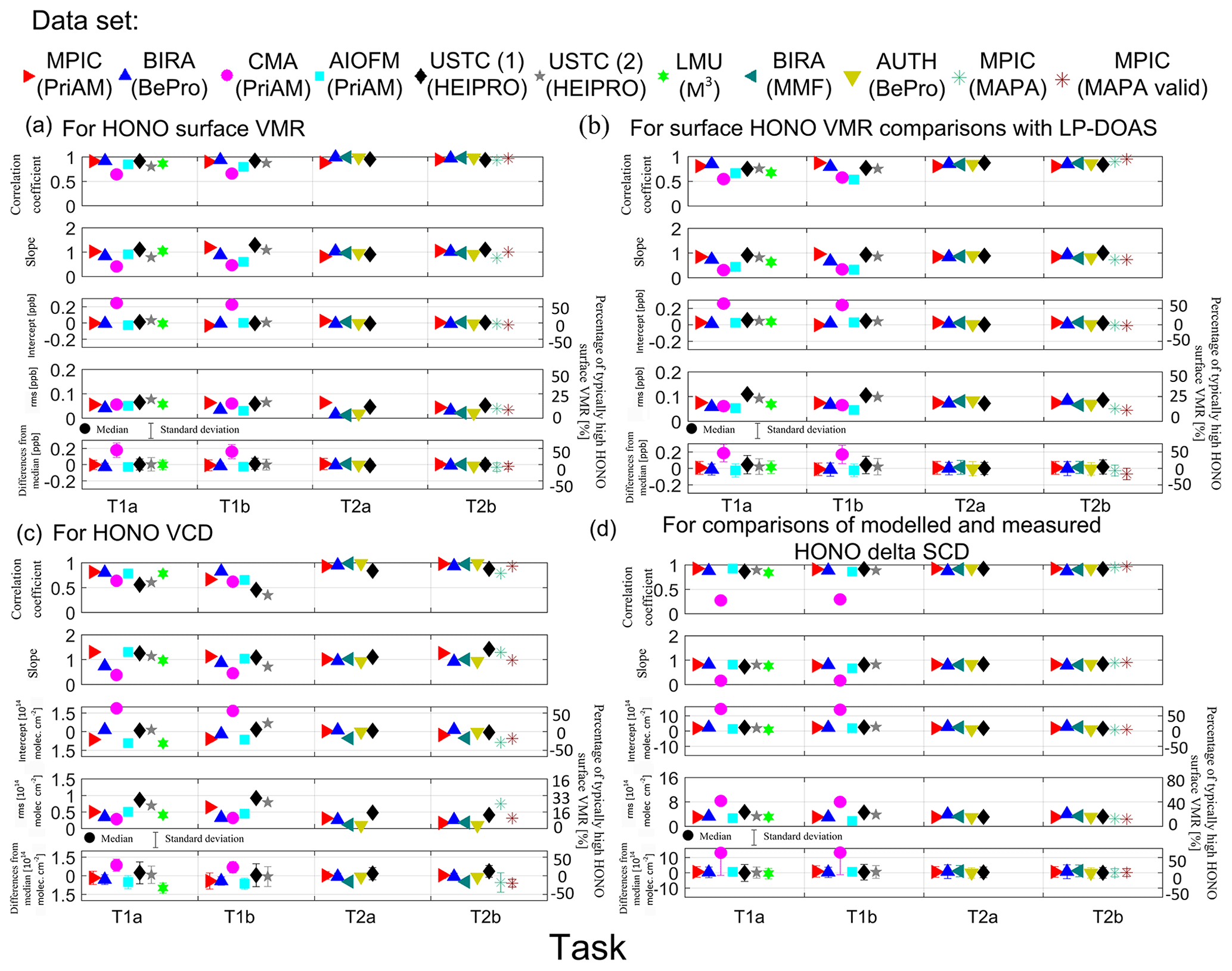
Figure 7 Correlation coefficients, slopes, intercepts, and rms of the residuals of the linear regression as well as median differences between individual participants and the reference values, which are the median values of all MAX-DOAS (a, c), and of the co-located LP-DOAS measurements (b). Comparisons of the near-surface HONO VMRs are given in (a) and (b). Comparisons of HONO VCDs are given in (c). For the individual data sets, the same comparison parameters are derived for the comparison of measured and modelled HONO delta SCDs (d).

4.3.1 Random discrepancies

The rms of the differences shown in Fig. 7a and c indicates systematically smaller random discrepancies for tasks T2a and T2b than for tasks T1a and T1b. The rms values of near-surface HONO VMRs are around 0.08 ppb (∼20 %) for all the data sets in tasks T1a and T1b. The rms values of HONO VCDs are around 0.6×10¹⁴ molec. cm⁻² (∼20 %) for most of the data sets, with a maximum value of $\sim \mathrm{0.9}\times {\mathrm{10}}^{\mathrm{14}}$ molec. (∼30 %) found for USTC (1). In tasks T2a and T2b, the rms for the near-surface HONO VMRs and VCDs is typically around 0.02 ppb (∼5 %) and 0.2×10¹⁴ molec. cm⁻² (∼7 %), respectively. The largest rms values of the near-surface HONO VMRs and VCDs are 0.06 ppb (∼15 %) and 0.7×10¹⁴ molec. (∼25 %), respectively, which are found for “MPIC (PriAM)” and “MPIC (MAPA)”. However, the rms decreases dramatically if quality flags are applied to the “MPIC (MAPA)” data to derive the “MPIC (MAPA valid)” data. The standard deviations of the differences of the vertical profiles against the median values shown in Fig. 8 indicate that the random discrepancies at altitudes above 0.2 km are mostly much smaller than close to the surface. The standard deviation is mostly around 0.02 ppb in the altitude grid of 0.2 to 0.4 km and almost zero at altitudes above 0.4 km. A relatively large deviation of ∼0.15 ppb for “AIOFM” appears at high altitudes in task T1a, and significantly larger deviations at high altitudes are found for the “MPIC (MAPA)” data than the other data in task T2b. However, the quality-controlled “MPIC (MAPA valid)” data show similar deviations to the other data.

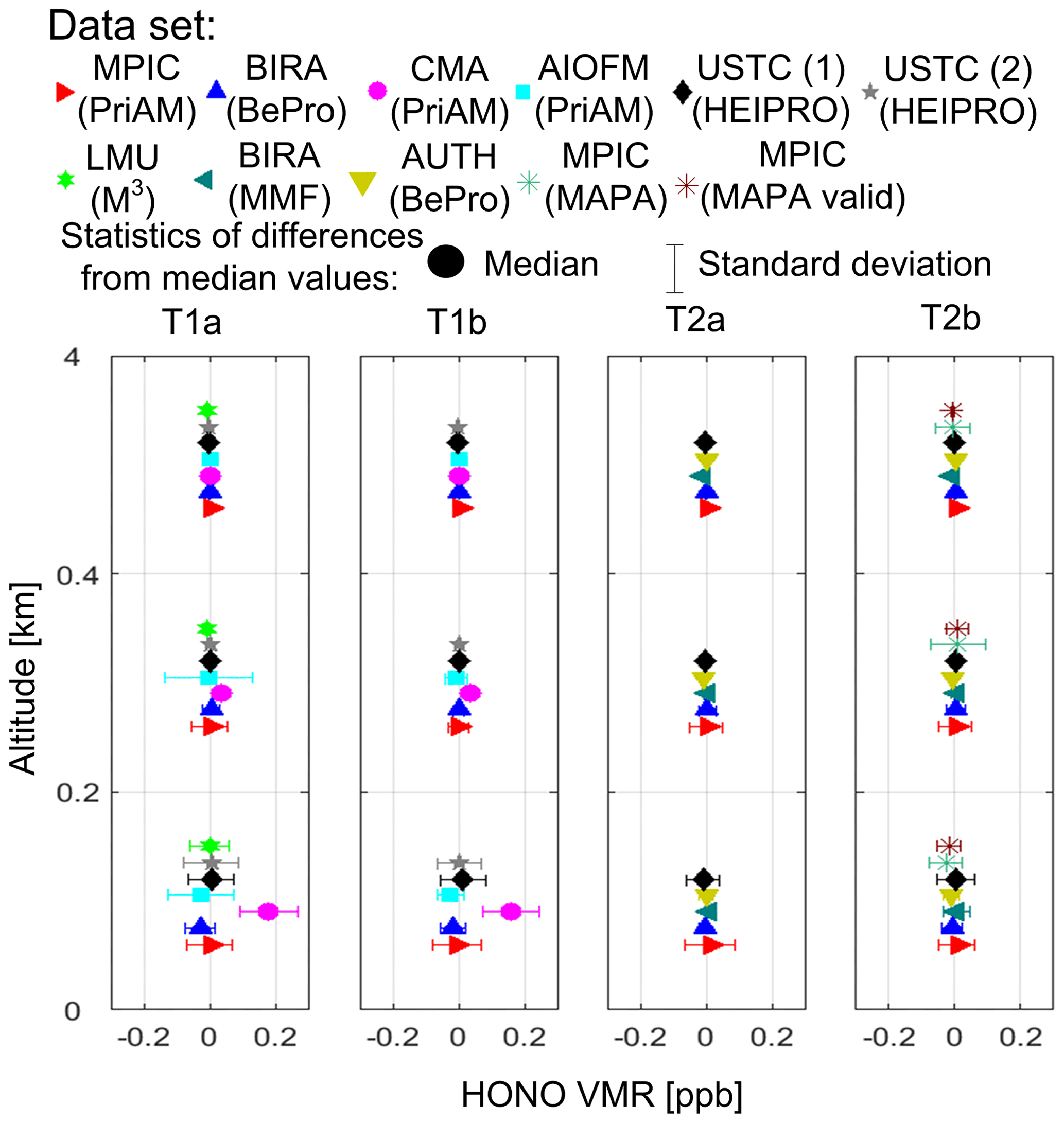
Figure 8 Median and standard deviations of the differences of the HONO VMR profiles derived from the individual participants compared to median values of all MAX-DOAS data for the whole campaign. The results in the vertical grids of 0 to 0.2 km, 0.2 to 0.4 km, and 0.4 to 4 km are shown as three vertical clusters of dots in the figures. Different subfigures represent results for different tasks.

4.3.2 Systematic discrepancies

Figure 7a and c show the median differences, intercepts, and slopes derived from the comparison of the HONO near-surface VMRs and VCDs. Similar to the HONO delta SCDs discussed in Sect. 3.3.2, the overall systematic discrepancies of near-surface VMRs and VCDs for low and high values are indicated by the slopes and intercepts, respectively. The median differences indicate that the systematic discrepancies are mostly in the range of 20 % for both tasks T1a and T1b and 5 % for both tasks T2a and T2b. The discrepancies of the VCDs are larger between the different data sets compared to the discrepancies of the near-surface VMRs, and the correlation coefficients of the comparisons of the VCDs are smaller than those of the comparisons of the near-surface VMRs. The near-surface VMRs are thus more consistent within the data sets than the VCDs. In addition, the discrepancies for tasks T1a and T1b are 4 times larger than for tasks T2a and T2b, which indicates that the discrepancies of the profile retrievals are dominated by the errors from the input HONO delta SCDs and not by the profile inversion algorithms. Additionally, the similar levels of discrepancies between tasks T1a and T1b and tasks T2a and T2b indicate that the effects of the “FRS” selection and different aerosol retrievals on the discrepancies of the HONO profile retrievals are almost negligible.

The data sets with substantial systematic discrepancies will be discussed individually in the following. The “CMA” data sets show a systematic overestimation of up to ∼45 % compared to the median values. However, Fig. 3e indicates a systematic underestimation of the “CMA” delta SCDs compared with the median values. Since Fig. 7d indicates a significant systematic overestimation of the modelled HONO delta SCDs compared to the measured ones, we conclude that the implementation of the profile inversions is the dominant factor causing a substantial overestimation of the “CMA” profile results compared to the other data. For the “LMU” data set, an overall underestimation of the VCDs, even though the near-surface VMRs are very consistent, is found because the VMRs are slightly lower than the median values at high altitudes, which can be seen in Fig. 8.

The systematic and random discrepancies between the different HONO profile results are quite comparable and typically in the range of 20 % for tasks T1a and T1b and 5 % for tasks T2a and T2b, with extreme discrepancies of ∼40 % for tasks T1a and T1b and ∼20 % for tasks T2a and T2b.

4.3.3 Comparison with LP-DOAS

The comparison results of the near-surface HONO VMRs of the individual participants against those measured by the co-located LP-DOAS instrument are displayed in Fig. 7b. There the correlation coefficients, slopes, intercepts, and rms of residuals derived from the linear regressions as well as the median differences against the LP-DOAS results are shown. The median differences and intercepts are consistent with those derived from the comparisons of the individual data sets against the median values (Fig. 7a). However, the slopes of the individual participants for tasks T1a and T1b are smaller than those derived from the comparisons against the median values (Fig. 7a). Therefore, in general all data sets systematically underestimate high near-surface HONO VMRs compared to the LP-DOAS results. Since the vertical layer measured by the LP-DOAS is consistent with the lowest vertical layer of the MAX-DOAS profile retrieval, the systematic differences might be mainly attributed to different air masses measured by the two techniques. It needs to be noted that MAX-DOAS typically measures the averaged HONO values in an effective light path of about 10 km, whereas LP-DOAS measures the averaged HONO values in a light path of about 4 km between its telescope and reflector. Since the typical lifetime of HONO is only of the order of 20 min under daytime conditions, strong HONO concentration horizontal inhomogeneities can be expected. However, the comparisons of NO₂ near-surface concentrations between MAX-DOAS measurements and LP-DOAS, as given in Tirpitz et al. (2020), do not indicate a systematic underestimation of MAX-DOAS. The different feature for NO₂ and HONO might be attributed to the much shorter lifetime of HONO than NO₂.

For the random differences of the individual data sets against the LP-DOAS measurements, in general similar rms values are observed to those derived from the comparison against the median values (Fig. 7a) for tasks T1a and T1b. However, for tasks T2a and T2b, the rms values for “BIRA”, “BIRA MMF”, and “AUTH” are much larger for the comparison with LP-DOAS than those for the comparison with the median values. Therefore, we conclude that the random discrepancies might be dominated by variations of HONO concentrations in the air mass measured by the LP-DOAS. Frequent variations of HONO concentrations can be expected due to the short lifetime of HONO. The variations of HONO concentrations in the air mass measured by the MAX-DOAS instrument can be smoothed due to the averaging effect in a typical effective light path of ∼10 km length.

5 Sensitivity studies of profile inversion

5.1 Sensitivity study on the effects of a priori profiles and the a priori covariance based on synthetic HONO delta SCDs

In this section we evaluate the influence of the a priori profile on the retrieval results based on synthetic HONO delta SCDs simulated by the RTM SCIATRAN. For these simulations, three different HONO profiles are used. These profiles as well as the other input parameters used for the RTM simulations are provided in Sect. 2.3.4. Among the three participants of this sensitivity study, “INTA” and “AUTH” used the “BePro” profile inversion algorithm, whereas “MPIC” used the “PriAM” profile inversion algorithm. While “BePro” uses a linear optimal estimation method, in “PriAM” a non-linear optimal estimation approach in logarithmic space is applied. We also evaluate the effect of different definitions of a priori covariance (S_a). In the baseline setting, S_a is set to 100 % of the a priori values for the diagonal terms. In the following this baseline configuration of S_a is referred to as “a priori determined S_a”. For the “BePro” algorithm, S_a is alternatively also set to a constant value at all altitudes, which is 100 % of the a priori value in the lowest altitude grid. This setting of S_a is referred to as the “constant S_a”. The alternative choice of S_a can theoretically decrease the constraints of the a priori profile on the retrieved profiles. Here it should be noted that for “PriAM” the definition of S_a according to the baseline settings is changed to unity at all altitudes due to its conversion to the logarithmic space. We do not apply an alternative S_a for “PriAM”.

HONO profiles are retrieved from synthetic HONO delta SCDs using three different a priori profiles (shown in Fig. 1b) and two different S_a. The retrieved profiles are shown in Fig. 9 separately for the three different algorithms. It is found that for all scenarios similar results are retrieved by “INTA” and “AUTH”, which apply the same “BePro” algorithm. For the tests with the a priori determined S_a, both “INTA” and “AUTH” considerably overestimate the HONO VMRs near the surface and underestimate those at high altitudes for profiles 2 and 3 if a priori profile 3 is used. However, for the tests with constant S_a, very consistent profile results are derived by “INTA” and “AUTH” for all three a priori profiles. This indicates that the HONO profile retrievals using “BePro” respond to the true HONO profiles much better if a “constant S_a” is used. For the “MPIC” results with the “PriAM” algorithm, very consistent profiles are also obtained for the three different a priori profiles. For profile 1 the “MPIC” retrieval agrees much better with the true profile than “INTA” and “AUTH” results. These results indicate that the “PriAM” algorithm can better respond to different HONO profile shapes through the implementation of the non-linear iterative procedure in logarithmic space. In addition, it needs to be clarified that negative values are allowed to be derived using “BePro”, although they are unrealistic in the real atmosphere. In contrast, negative values are avoided in the “PriAM” algorithm due to the logarithmic transformation.

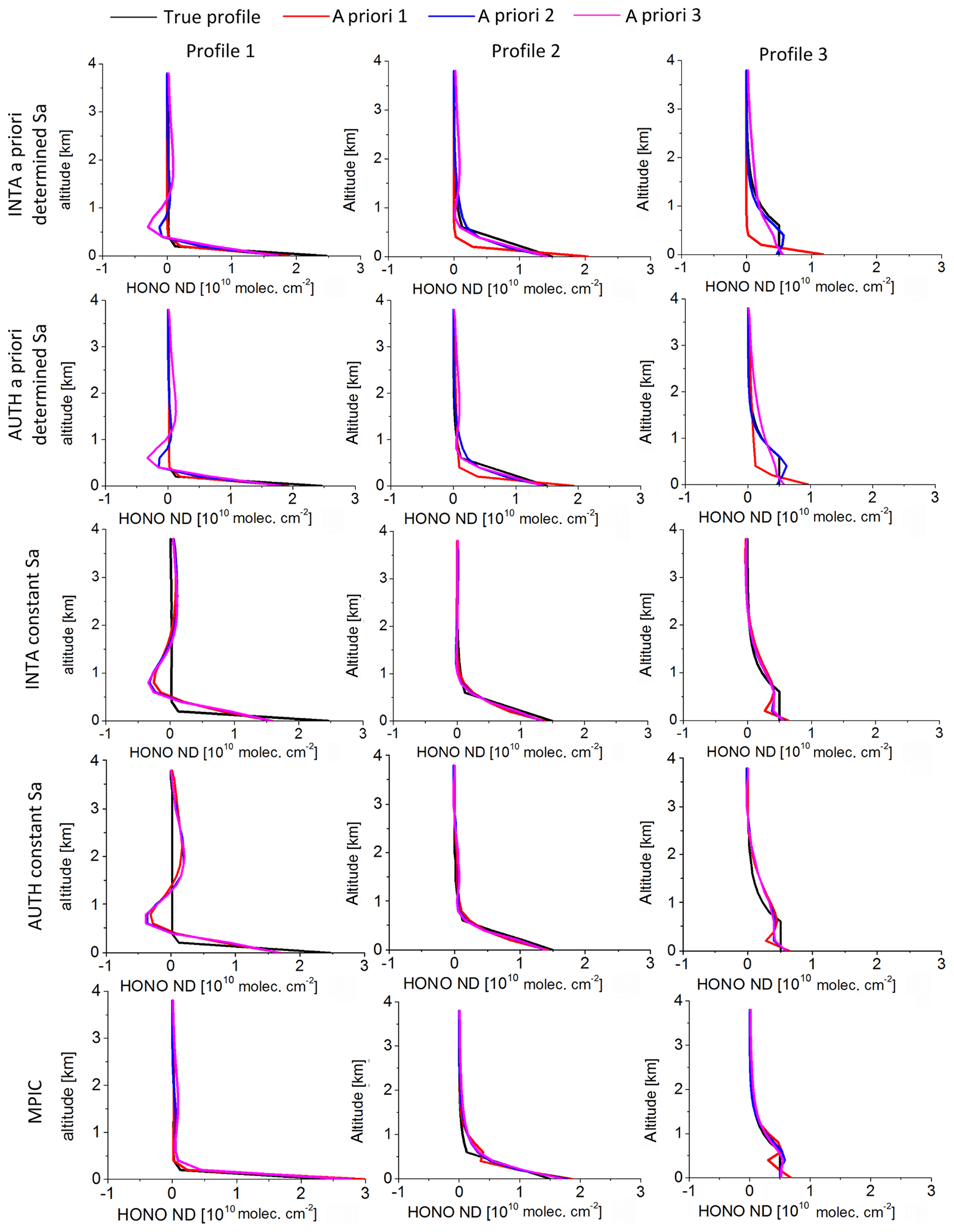
Figure 9 HONO profiles retrieved from simulated HONO delta SCDs by the different participants using different inversion algorithms with “constant Sa” and “a priori determined Sa” (see text). The black curves in the different columns of the figure indicate the different input profiles, and the other colours indicate the profiles retrieved using different a priori profiles (see Fig. 1b).

The effects of random noise on the profile retrievals were tested based on the “noisy synthetic HONO delta SCDs”, which are described in Sect. 2.3.4. Median values and standard deviations of differences of the retrieved HONO profiles compared to those retrieved from the synthetic HONO delta SCDs without noise are shown in Fig. 10, and for the same results, the ratios of the median values and standard deviations shown in Fig. 10 compared to the true HONO profiles are plotted in Fig. 11. The results for the retrievals using the “a priori determined S_a” and “constant S_a” are shown separately in Figs. 10 and 11. For “INTA” and “AUTH”, much larger standard deviations for retrievals using the “constant S_a” than those using the “a priori determined S_a” at high altitudes are found due to the smaller a priori constraints if the “constant S_a” is used. For “MPIC”, standard deviations at altitudes below 1 km are similar to those for “INTA” and “AUTH” with the “constant S_a”. However, much smaller standard deviations are found at altitudes above 1 km.

Figure 10 Median and standard deviations of the differences of the HONO VMR profiles retrieved from the simulated HONO delta SCDs with added artificial noise compared to those without noise by the different participants using a different inversion algorithm with “constant Sa” and “a priori determined Sa” (see text). The root mean square of the noise is 3×10¹⁴ molec. cm⁻². The different colours indicate the results for the three different assumed HONO profiles.

We conclude that for the “BePro” algorithm, the “constant S_a” can increase the response of the profile retrievals to different HONO profile shapes but can reduce the stability. The “PriAM” algorithm can balance the response and stability well. Therefore we recommend retrieving HONO profiles in logarithmic space.

5.2 Sensitivity study on the effects of the grid intervals in the profile retrievals

In the baseline settings of the profile retrievals the grid intervals were set to 200 m. Since a significant vertical gradient might appear in the lowest 200 m, we tested the effects of using different grid intervals, e.g. 50 and 100 m, on the retrieved profiles using the “PriAM” algorithm based on the “MPIC”-measured HONO delta SCDs during the whole campaign. For different grid intervals, the averaged diurnal variations of the retrieved HONO VMRs below 200 m are shown in Fig. 12a. Differences of the retrieved HONO VMRs using grid intervals of 100 and 50 m compared to the baseline setting are shown in Fig. 12b. Figure 12 indicates that the retrieved HONO VMRs below 100 m for both retrievals with grid intervals of 50 and 100 m are similar to those grid intervals of 200 m (baseline settings). The retrieved HONO VMRs significantly decrease in the grids above 100 m. Based on this sensitivity test, it is concluded that a finer resolution than 200 m can improve the profile results in the altitude range below 200 m.

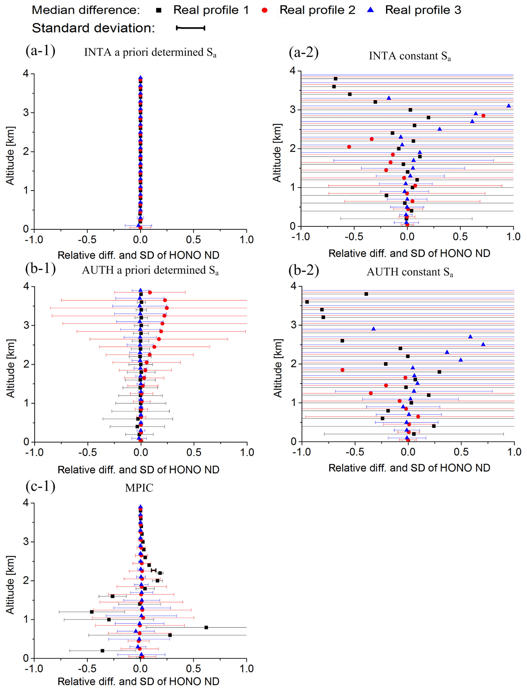
Figure 11 Median and standard deviations of the relative differences of the HONO VMR profiles retrieved from the simulated HONO delta SCDs with added artificial noise compared to those without noise by the different participants using a different inversion algorithm with “constant Sa” and “a priori determined Sa” (see text).

5.3 Measurement uncertainties of HONO dSCDs and their effects on profile retrievals

In order to calculate the diagonal elements of the covariance matrix of measurement uncertainties for profile retrievals using the optimal estimation method, measurement uncertainties of HONO dSCDs need to be estimated. Measurement uncertainties can be mainly attributed to instrumental noise and atmospheric variability. DOAS fit errors provide a good representation of the instrumental noise. In the baseline settings of profile retrievals, we assume that measurement uncertainties and DOAS fit errors of HONO dSCDs are equivalent. However, this assumption is not realistic if the effect of atmospheric variability is significantly larger than DOAS fit errors. As shown in Fig. 3f, the lowest DOAS fit errors of $\sim \mathrm{0.1}\times {\mathrm{10}}^{\mathrm{15}}$ molec. cm⁻² are found for the BIRA instrument, and they are 3 times lower than the typical DOAS fit error of $\sim \mathrm{0.3}\times {\mathrm{10}}^{\mathrm{15}}$ molec. cm⁻² of the other instruments as shown in Fig. 2c. Two data sets of HONO profile results are derived from the same HONO dSCD data sets with different settings of the diagonal elements of the measurement uncertainty covariance matrix. The baseline profile retrieval settings (i.e. 100 % of the DOAS fit errors of the HONO dSCDs) are applied for the retrievals of the “BIRA (v1)” data set, while the “BIRA (v2)” data set corresponds to the BePRO profile retrievals where 300 % of the DOAS fit errors of the HONO dSCDs is used. Figure 5 indicates that the “BIRA (v1)” results deviate more from the median values than those of “BIRA (v2)”. This feature is due to the fact that the measurement uncertainties of the “BIRA” instrument are substantially larger than its DOAS fit errors, due to the effect of atmospheric variability. In order to realistically estimate measurement uncertainties, the standard deviations of the “BIRA” HONO dSCDs retrieved using the daily noon FRS in the time period of 11:00 to 16:00 UTC on individual days are shown in Fig. 13a. Since HONO dSCDs, especially in the zenith view, are close to zero as shown in Fig. 2b, the standard deviations can represent random measurement uncertainties. Since the DOAS fit errors of the “MPIC” data set are in the moderate range of all the participating instruments, the standard deviations of the “MPIC” data set are calculated and shown in Fig. 13b for comparisons with the “BIRA” data set. In addition, the averaged DOAS fit errors of HONO dSCDs of both data sets are shown in Fig. 13c, d. Figure 13 indicates that although the DOAS fit errors of the “BIRA” data set are about one-third of the “MPIC” data set, the standard deviations of both the “MPIC” and “BIRA” data sets are comparable and around 0.2 to 0.3×10¹⁵ molec. cm⁻². This feature suggests that measurement uncertainties are similar for both the “MPIC” and “BIRA” data sets due to the dominant effect of atmospheric variability on the measurement uncertainties of the “BIRA” data set. In contrast to the “BIRA” case, both atmospheric variability and instrumental noise are comparable in the “MPIC” data set. Since the measurement uncertainties are about 3 times higher than the DOAS fit errors for the “BIRA” instrument, the setting for the “BIRA (v2)” profile results is more realistic that for the “BIRA (v1)” profile results. However, for the “MPIC” instrument and most of the other instruments, since the measurement uncertainties are comparable to the DOAS fit errors, baseline settings are reasonable. We can conclude that not only DOAS fit errors, but also atmospheric variability should be considered for the estimation of measurement uncertainties for profile retrievals. The effect of atmospheric variability on measurement uncertainties of HONO dSCDs is roughly around 0.2 to 0.3×10¹⁵ molec. cm⁻², which might be significantly larger than DOAS fit errors of a state-of-the-art MAX-DOAS instrument with high signal-to-noise ratios.

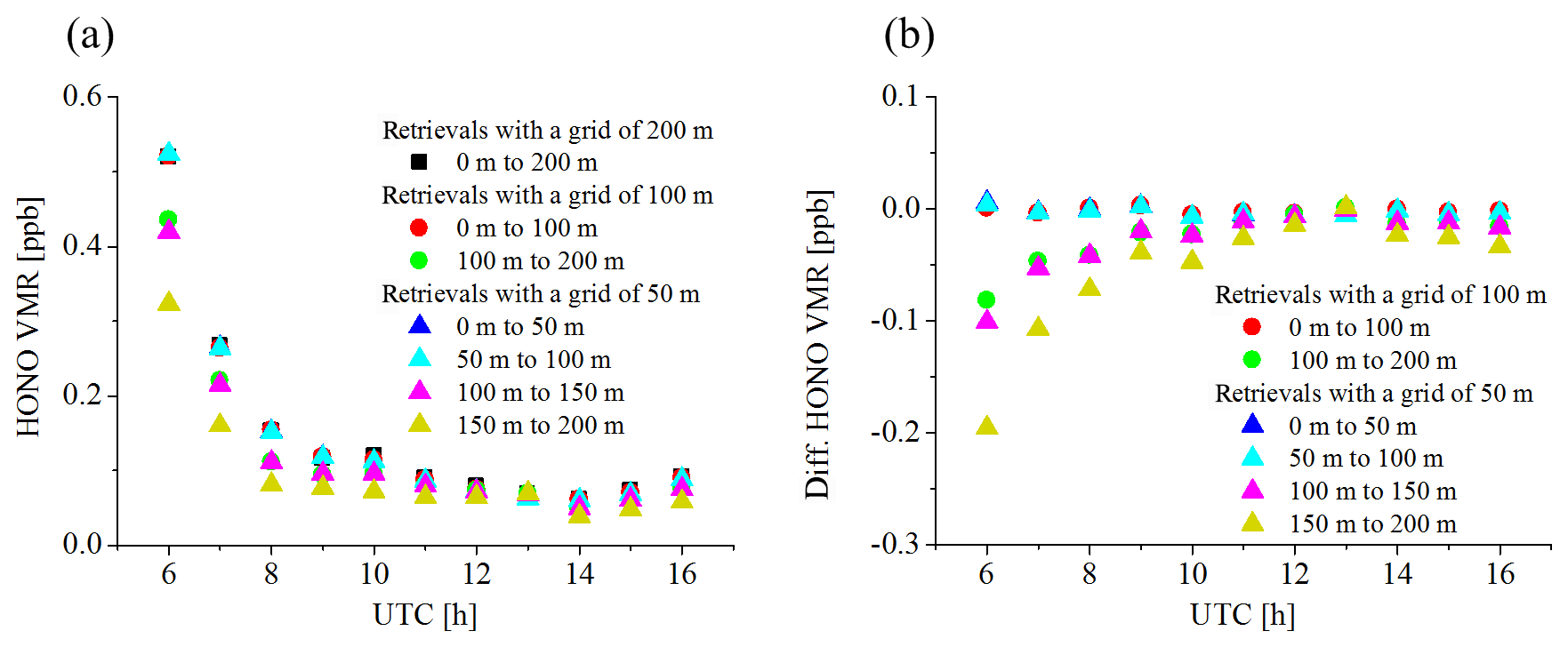
Figure 12 (a) Averaged diurnal variations of the HONO VMRs in the altitude range of up to 200 m retrieved using the “PriAM” algorithm using vertical grid intervals of 50, 100, and 200 m, respectively. Note that the results in the altitude grids below 200 m are given, respectively. The results are derived from the HONO delta SCD measured by the MPIC instrument. (b) Averaged diurnal variations of the differences of the HONO VMRs retrieved for vertical grid intervals of 50 m and 100 m compared to those retrieved for the vertical grid interval of 200 m.

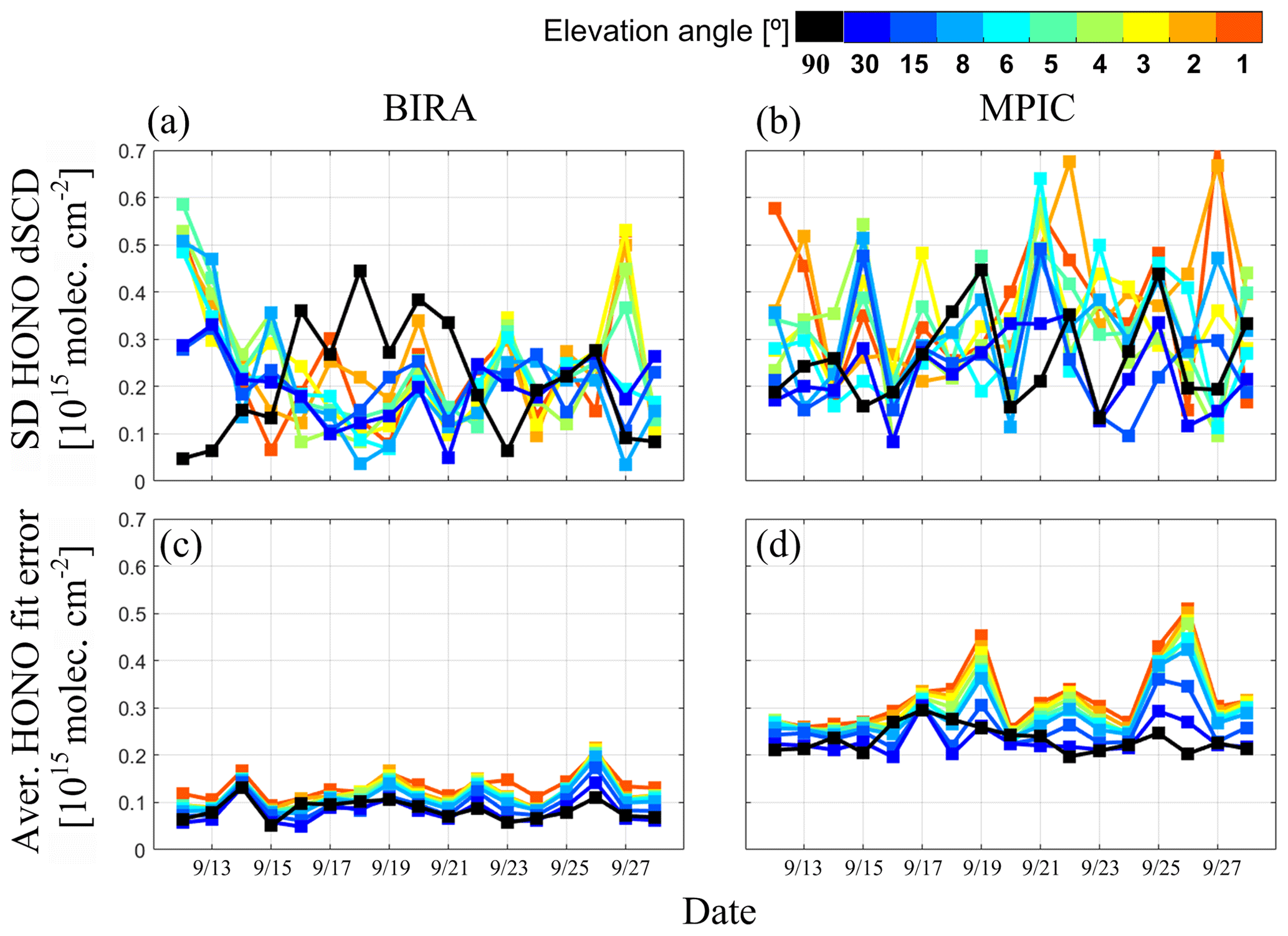
Figure 13 Standard deviations (a, b) and averaged DOAS fit errors (c, d) of HONO dSCDs retrieved using the daily noon FRS in the time period of 11:00 to 16:00 UTC for individual days for the BIRA (a, c) and MPIC (b, d) instruments, respectively. The colour map indicates elevation angles.

6 Conclusions

In this study, HONO delta SCDs and vertical profiles are retrieved from different MAX-DOAS observations during the CINDI-2 campaign. VCDs and near-surface VMRs are derived using different profile inversion algorithms, which are applied to HONO delta SCDs analysed by the different participants. Peak HONO values with delta SCDs at 1^∘ elevation angle of $\sim \mathrm{3}\times {\mathrm{10}}^{\mathrm{15}}$ molec., VCDs of 3×10¹⁴ molec. cm⁻², and near-surface VMRs of 0.4 ppb on average are retrieved in the early morning. These are followed by a steep decrease to $\sim \mathrm{1.2}\times {\mathrm{10}}^{\mathrm{15}}$ molec. cm⁻², $\sim \mathrm{1.5}\times {\mathrm{10}}^{\mathrm{14}}$ molec. cm⁻², and ∼0.1 ppb, respectively, during the period from 06:00 to 08:00 UTC. Afterwards, the HONO values stay low and further decrease slightly during the rest of the day. The profile results indicate that most of the HONO accumulates at altitudes below 0.2 km, and HONO concentrations are close to zero at altitudes above 0.4 km during the day.

We evaluated random and systematic differences between different retrieval results of HONO delta SCDs derived from different MAX-DOAS instruments using different inversion algorithms. It needs to be clarified that the data samplings are limited in the statistic study, and thus the uncertainties of the HONO delta SCDs (and other HONO results including VCDs, near-surface VMRs, and profiles) can only be roughly estimated for typical cases. For MAX-DOAS instruments with moderate performance during this campaign, the systematic discrepancies of the delta SCDs of the different MAX-DOAS instruments are generally in the range of $\pm \mathrm{0.3}\times {\mathrm{10}}^{\mathrm{15}}$ molec. cm⁻², which is half of the typical random uncertainty of $\sim \mathrm{0.6}\times {\mathrm{10}}^{\mathrm{15}}$ molec. cm⁻². For a typical high value of HONO delta SCD of 2×10¹⁵ molec. cm⁻², the typical relative systematic and random uncertainties are about 15 % and 30 %, respectively. Similar magnitudes of random and systematic uncertainties are observed for different elevation angles. However, since the HONO delta SCDs decrease with increasing elevation angle, the relative random and systematic uncertainties reach up to 200 %–400 % and 100 %–200 %, respectively, for the 30^∘ elevation angle. The HONO delta SCDs retrieved by some participants show substantially larger random and systematic discrepancies compared to most participants, which is mainly caused by limitations of the instrumental signal-to-noise ratios or an inappropriate implementation of DOAS fits. Another important finding is that for most instruments the random discrepancies of HONO delta SCD results between the different instruments are significantly larger than individual DOAS fit errors due to the effects of atmospheric variability and discrepancies of instrumental FOV and acquisition time. In addition, for most of the instruments, the effects of using either a “sequential FRS” or “daily noon FRS” on the errors of the HONO delta SCDs are practically negligible, with systematic and random differences between both retrieval results typically within $\pm \mathrm{0.1}\times {\mathrm{10}}^{\mathrm{15}}$ molec. cm⁻² ($\sim \pm \mathrm{5}$ %).

Random and systematic differences between the retrieved HONO VCDs, near-surface VMRs, and profiles from the different MAX-DOAS instruments and inversion algorithms are further evaluated via statistical inter-comparison. Both systematic and random differences of HONO VCDs and near-surface VMRs are typically ∼20 %. For some instruments, the maximum random and systematic discrepancies are ∼40 %. In order to better understand the reasons for the differences, all participants also retrieved HONO profiles from a set of common HONO delta SCDs using their specific inversion algorithms. The results of this task indicate that the differences of the profile inversion algorithms generally contribute to both systematic and random discrepancies of the HONO VCDs at about $\sim \pm \mathrm{0.2}\times {\mathrm{10}}^{\mathrm{14}}$ molec. cm⁻² and of the near-surface VMRs at about $\sim \pm \mathrm{0.02}$ ppb (typically ∼5 % for both VCDs and near-surface VMRs). These results indicate that the errors of the HONO delta SCDs dominate the differences of HONO profile results. Further error sources, especially for the most extreme discrepancies, are probably inappropriate implementations of the profile inversion algorithms and/or configurations of the profile retrievals. Both systematic and random discrepancies are considerably higher in the lowest altitude range of 0 to 0.2 km, mostly ∼0.02 ppb in the altitude range from 0.2 to 0.4 km, and almost zero above. In addition, the effect of using a “daily noon FRS” or a “sequential FRS” in the DOAS fit on the profile results is almost negligible. Also, the effect of different aerosol retrievals on HONO profile results is typically negligible.

The near-surface HONO VMRs retrieved from different MAX-DOAS measurements are also compared to the co-located LP-DOAS measurements. In general, the systematic discrepancies of the individual MAX-DOAS measurements compared to the LP-DOAS results are similar to those derived from the comparison with the median values of all MAX-DOAS results. Interestingly, the median values of all MAX-DOAS measurements are systematically lower or higher than the LP-DOAS results by up to 0.15 ppb (∼50 %) and 0.07 ppb (∼20 %–200 %) in the early morning and around noon, respectively.

The effects of a priori profiles and covariance for the “BePro” and “PriAM” profile inversion algorithms, which are both based on the optimal estimation method but in linear and logarithmic space, respectively, were evaluated using simulated delta SCDs for three different altitude profiles. The results of this sensitivity study indicate that a “constant Sa” for the “BePro” algorithm in linear space can increase the response of the profile retrievals to different HONO profile shapes but tends to reduce the stability. The “PriAM” algorithm in logarithmic space can balance the response and stability well. Therefore we recommend retrieving HONO profiles in logarithmic space. Additional sensitivity tests indicate that a finer resolution than 200 m improves the retrieved profiles in the altitude range below 200 m. In addition it is found that measurement uncertainties of HONO dSCDs, which are needed to calculate the measurement uncertainty covariance matrix for profile retrievals using the optimal estimation method, can be significantly larger than DOAS fit errors due to the effect of atmospheric variability, especially for an instrument with a low noise level. This may lead to unrealistic estimations of measurement uncertainties causing considerable discrepancies in profile results. Therefore, not only DOAS fit errors, but also the effect of atmospheric variability, need to be considered for the estimation of measurement uncertainties. The typical contribution of atmospheric variability to measurement uncertainties of HONO dSCDs is about 2 to 3×10¹⁴ molec. cm⁻², but it might depend on particular sky conditions and instrumental properties.

We summarize that, even though the errors of the measured HONO delta SCDs usually dominate the errors of the retrieved HONO profiles, the inappropriate implementation of the profile inversion algorithms can also cause substantial discrepancies. Profile inversion algorithms with proper configuration can retrieve different HONO profile shapes well, especially in logarithmic space. This confirms that one important feature of the retrieved HONO profiles, the high concentrations near the surface, represents the ambient HONO vertical distribution well during the CINDI-2 campaign.