the Creative Commons Attribution 4.0 License.
the Creative Commons Attribution 4.0 License.
 | 02 Oct 2020
Assessment of global total column water vapor sounding using a spaceborne differential absorption radar
Richard Roy
Matthew Lebsock
The feasibility of using a differential absorption radar (DAR) to retrieve total column water vapor from space is investigated. DAR combines at least two radar tones near an absorption line, in this case a water vapor line, to measure humidity information from the differential absorption “on” and “off” the line. From a spaceborne platform, DAR can be used to retrieve total column water vapor by measuring the differential reflection from the Earth's surface. We assess the expected precision, yield, and potential biases of retrieved total column water vapor values by applying an end-to-end radar instrument simulator to near-global weather analysis fields collocated with CloudSat measurements. The approach allows us to characterize the DAR performance across a globally representative dataset of atmospheric conditions including clouds and precipitation as well as different surface types.
We assume a hypothetical spaceborne G-band radar with pulse compression orbiting the Earth at 405 km with a 1 m antenna, equivalent to a footprint diameter of 850, and 500 m horizontal integration. The simulations include the scattering effects of rain, snow, as well as liquid and ice clouds, spectroscopic uncertainties, and uncertainties due to the initial assumed water vapor profile. Results indicate that using two radar tones at 167 and 174.8 GHz with a transmit power of 20 W ensures that both pulses will be detected with a signal-to-noise ratio greater than 1 at least 70 % of the time in the tropics and more than 90 % of the time outside the tropics and that total column water vapor can be retrieved with a precision better than 1.3 mm.
- Article
(13878 KB) - Full-text XML
- BibTeX
- EndNote


Water vapor is one of the most important gases in the Earth's atmosphere. Its relevance has led to the development of several techniques for measuring its vertical distribution as well as the vertically integrated atmospheric water vapor content, which is often referred to as precipitable water, total water vapor, integrated water vapor, integrated precipitable water vapor, or total column water vapor. The Global Climate Observing System has highlighted the utility of total column water vapor observations, declaring it as an essential climate variable (GCOS-ECV, 2020), which the World Meteorological Organization defines as a physical, chemical, or biological variable that critically contributes to the characterization of Earth's climate.
Passive satellite total column water vapor retrievals typically use instruments that measure in the visible (e.g., Lang et al., 2007; Wang et al., 2014), near-infrared (e.g., Lindstrot et al., 2012; Diedrich et al., 2015; Nelson et al., 2016), infrared (e.g., Pougatchev et al., 2009; Bedka et al., 2010), and microwave spectral regions (e.g., Schluessel and Emery, 1990; Wentz, 1997). However, each spectral region has its limitations: visible and near-infrared measurements are limited to cloud-free daytime regions and to land areas where the relatively bright surface reflection increases the signal compared to the dark ocean surfaces; infrared and microwave measurements can operate only over ice-free oceans, where the surface emissivity is well characterized. Additionally, infrared measurements are not possible in the presence of clouds or rain.
This study explores the feasibility of using a differential absorption radar (DAR) to remotely measure total column water vapor under all sky conditions, for all surface types and during day and night. The DAR technique is analogous to the differential absorption lidar (DIAL) technique (e.g., Schotland, 1966; Browell et al., 1979; Wulfmeyer and Walther, 2001) but operates in the microwave or millimeter-wave regime. In essence, the difference between the radar reflectivity at two nearby frequencies, “on” and “off” an absorption line, can be related to the amount of absorbing gas between the radar and the scattering target, which in this case is the Earth's surface.
Prior studies have shown that the DAR technique can be used to derive water vapor profiles using three frequencies around 22 GHz (Meneghini et al., 2005) and two frequencies at around 10 and 94 GHz (Tian et al., 2007) or at 2.8 and 35 GHz (Ellis and Vivekanandan, 2010). However, these studies require distinct radar transmitters for each frequency, which complicates the DAR measurement due to independent system calibration and beam overlap issues. Lebsock et al. (2015), Millán et al. (2016), and Battaglia and Kollias (2019) explored the feasibility of water vapor profiling with a narrow-band transmitter on the wings of the 183 GHz water vapor line, in which case the DAR measurement can be made with a single transceiver, greatly simplifying the measurement interpretation.
With respect to remotely measuring total column water vapor, Lebsock et al. (2015) and Millán et al. (2016) assessed the feasibility of using two frequencies near the 183 GHz water absorption line and using large eddy simulations and global cloud observations from CloudSat (Stephens et al., 2002), respectively. These studies concluded that the DAR technique could provide nearly spatially continuous observations of total column water vapor, even under rainy conditions. However, both studies assumed a constant instrument error model, with a 0.16 dBZ radar precision and around a −30 dBZ minimum detectable signal. Here we use a more realistic uncertainty model (described in Sect. 2) that includes speckle noise, that is, that depends on the magnitude of the return power, which in turn depends on the water vapor burden. Furthermore, their simulations explored frequencies prohibited by the Federal Communications Commission for spaceborne transmission.
Here, we assume a frequency-chirp, pulsed radar system, similar to the proof-of-concept instrument described by Cooper et al. (2018) and by Roy et al. (2018). Currently, a similar airborne radar operating near 170 GHz is being developed and has recently been validated during a ground-based deployment (Roy et al., 2019). The motivation of this study is to investigate the transmit power necessary to achieve close to global total column water vapor measurements from a space platform given realistic instrument and orbital parameters and using frequencies that could be available for space transmission.
It has been shown (Lebsock et al., 2015; Millán et al., 2016) that the ratio of two surface returns can be used to estimate the total column water vapor. Nevertheless, for completeness, a description of the radar theory is summarized here. Neglecting multiple scattering, the surface return power measured by a monostatic radar which transmits a power PT at a given frequency ν is given by
where G(ν) is the antenna gain, r is the distance to the surface, Ω(ν) is the integral of the normalized two-way antenna pattern, and σ0(ν) is the normalized surface cross section. Υ2(ν) is the two-way transmission given by
where σgas(ν,r) represents the gaseous absorption coefficient and σPext(ν,r) the particulate extinction (the sum of absorption and scattering) coefficient along the radar path.
If two radar tones are measured simultaneously, the ratio of two surface returns can be expressed as
where C(ν) is the radar system parameter given by the first term of Eq. (1), that is, .
Assuming that the frequency dependence of σPext(ν,r) and σ0(ν) is small relative to that of σgas(ν,r), this equation becomes
which can be rewritten as
where ρ(r) is the air density and the sum is over all the absorbers with mass extinction cross section κi(ν,r) and volume mixing ratio vi(r). If the radar tones are close to a strong absorption line, the associated gas dominates the absorption. For example, absorption due to water vapor dominates the atmospheric attenuation near 183 GHz. In that scenario, the only unknowns remaining are pressure, temperature, and water vapor mixing ratio. It follows that, assuming a temperature and pressure profile (for example, from reanalysis fields or a climatology) and a water vapor profile shape, it should be possible to retrieve total column water vapor from the ratio of two surface returns. The uncertainties associated with these assumed profiles will be discussed in Sect. 5.2.
To explore the capabilities of this technique, the radar reflectivity uncertainty needs to be properly simulated. Here we assume a moving satellite platform with velocity V and antenna diameter D. Following Roy et al. (2018) and Roy et al. (2019), the uncertainty in the received power (see Eq. 1), assuming decorrelated pulses, is given by
where Np is the number of pulses used in each measurement of PR(ν). The first term is due to speckle noise, the second term is known as Townes noise (i.e., Townes and Geschwind, 1948; Pearson et al., 2008), and the last term is due to the instrument thermal noise PN. Speckle noise can be understood as the variation in backscatter from randomly distributed scatterers causing interference effects in the coherent measurement of the total returned electric field. In simple terms, Townes noise is due to the cross term of the sum of the signal and noise voltages. The instrument thermal noise is determined by
where kb is the Boltzmann constant, Tsys is the system noise temperature, and τ is the chirp time which we fix according to the relation given by (Walsh, 1982)
which ensures that sequential pulses are decorrelated.
The number of pulses is then determined by
where ς is the duty cycle, assumed to be 0.25 using a chirped pulse, and T is the total integration time available for each radar tone, estimated using
where ΔL is the desired along-track horizontal resolution and NT is the number of radar tones (e.g., at least two, for the online and offline tones).
In this study we assume a 405 km orbit, a 1 m antenna diameter, radar tones at 167 and 174.8 GHz, a system temperature of 1800 K, a desired horizontal integration of 500 m, and transmit powers varying from 0.1 to 100 W. These assumptions result in a footprint diameter of ∼850 m, a chirp time of 66 µs, a total incoherent integration time per tone of 33 ms, and 125 number of pulses. These radar characteristics are listed in Table 1 (which also includes the symbols used throughout this study). Further, we define the minimum detectable signal to be PR(ν)=PN (i.e., where a single-pulse signal-to-noise ratio (SNR) is equal to 1). This determines the sensitivity of the DAR measurement system. Despite the relatively long chirp time, we do not simulate any side lobes because, as demonstrated by RainCube (a Ka-band 6U cubesat radar with a 166 µs pulse length) through an optimal selection of pulse shape and digital processing, side lobes can be suppressed to accurately measure the most relevant precipitation processes near the surface (Peral et al., 2019).
Table 1Satellite radar parameters.
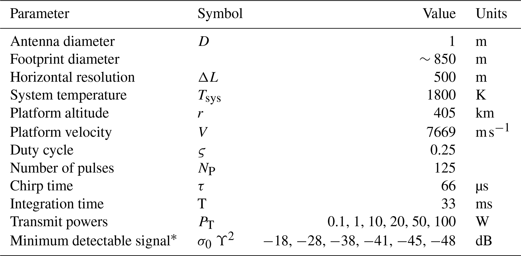
∗ For each of the transmit powers considered, respectively.
The Earth's surface is a bright target, meaning that the SNR should be large. In this scenario, PR(ν) is generally much larger than PN, and the last two terms of Eq. (6) (the contributions from the Townes noise and the instrument noise) are small. Thus, in high-SNR regimes the fractional uncertainty in the received power simply becomes .
Radar returns are simulated using the radiometric model described in Millán et al. (2014, 2016). In short, radar reflectivities are estimated using the time-dependent two-stream approximation (Hogan and Battaglia, 2008), gaseous absorption is evaluated using the clear-sky forward model for the EOS Microwave Limb Sounder (Read et al., 2004), hydrometeor scattering properties are evaluated using Mie scattering theory (assuming spherical solid hydrometeors), and the surface cross section is calculated using a quasi-specular scattering model (Li et al., 2005) for the ocean surface. More details, such as the dielectric constants and the particle size distributions used, can be found in Table 2.
Liebe et al. (1991)Hufford (1991)McFarquhar and Heymsfield (1997)Abel and Boutle (2012)Sekhon and Sirvastava (1970)Read et al. (2004)Hogan and Battaglia (2008); Hogan (2013)Li et al. (2005)Table 2Radar instrument simulator specifics.

∗ Particle size distribution.
The hydrometeor fields used in this study are supplied by cloud/rain profiles observed by CloudSat. CloudSat is a NASA satellite carrying a 94 GHz profiling radar sensitive to both cloud and precipitation particles (Stephens et al., 2002). CloudSat retrievals provide the hydrometeor information, while spatially and temporally interpolated weather analysis provides the meteorological conditions. In particular, rain and snow profiles are taken from the 2C-RAINPROFILE (Lebsock and L'Ecuyer, 2011) products and liquid water content (LWC) and ice water content (IWC) from the 2B-CWCRO R04 (Austin and Stephens, 2001; Austin et al., 2009). Temperature, pressure, and water vapor are taken from the European Centre for Medium-Range Weather Forecasts auxiliary (ECMWF-aux) products (Cronk and Partain, 2017). Note that to decrease the number of calculations, we subsample these fields; we only used 1 out of every 50 CloudSat measurements. In other words, we under-sample CloudSat to save computational time. It is noted that non-uniformities within the beam at scales smaller than the CloudSat horizontal resolution are not included in these simulations. They will be better addressed using either high-resolution ground-based data or high-resolution atmospheric models in subsequent studies.

Figure 1Example of CloudSat-driven simulations. (a) Hydrometeor burden. (b) Water vapor burden for two scenarios: the ECMWF-AUX scenario (solid line) and dry case (dash line). (c) CloudSat-driven simulations assuming the hydrometeor burden shown in (a) and the two water vapor burden scenarios (solid lines for the ECMWF-AUX scenario and dash lines for the dry case) shown in (b) for the two frequencies used in this study (half circles indicate the magnitude of the surface return in dBZ for the ECMWF-AUX scenario, while triangles indicate it for the dry case).
Figure 1 shows an example simulation at 167 and 174.8 GHz, which are the two frequencies used throughout this study. These frequencies are the extreme frequency values achievable due to international transmission restrictions (NTIA, 2015). The observed scene is heavily overcast with snow aloft and rain beneath the freezing level. The simulation is repeated for two distinct water vapor burdens; a wet atmosphere as estimated from the weather analysis and a hypothetical dry atmosphere (with 44 and 4 mm of total column water vapor burden and 298 and 257 K surface temperature, respectively). As expected, the dry atmosphere simulations show considerably less attenuation, but nevertheless, the impact of the water vapor burden is clearly visible in the extra attenuation experienced by the 174.8 GHz radar tone compared to 167 GHz. As examples of this burden, Fig. 2 shows the spectral variation of the surface return for different total column water vapor burdens under clear-sky conditions. The spectral contrast between 174.8 and 167 GHz varies from 0.1 dB for no water vapor to 31 dB for 60 mm of total column water vapor.
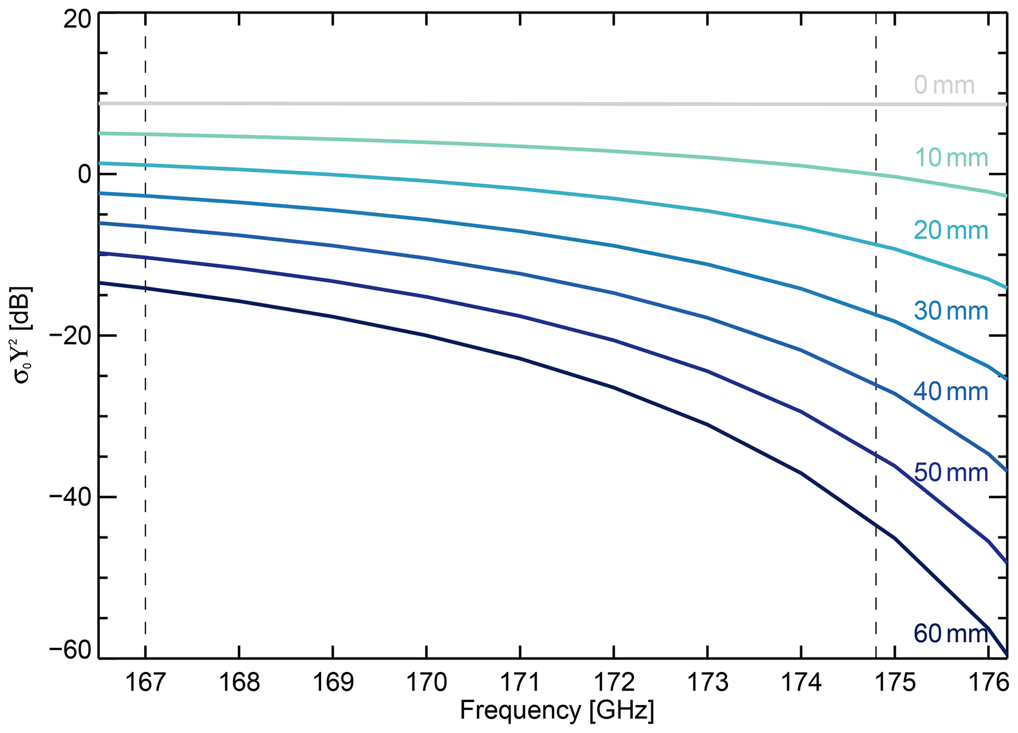
Figure 2Examples of the spectral variation of the column surface return due to several total column water vapor burdens under clear-sky conditions. Dashed vertical lines show the two frequencies used in this study (167 and 174.8 GHz).
We use a quasi-specular surface backscatter model over the oceans (Li et al., 2005) assuming monthly climatological values derived from the ERA-Interim reanalysis for near-surface wind speed and sea surface temperature (Dee et al., 2011). Over land surfaces there are no empirical models for the radar cross section at these frequencies. Therefore we use the observed cross sections from CloudSat to scale the ocean frequency dependence of the Li et al. (2005) model as follows:
where σ0(ν)′ is the modified surface cross section at a given frequency, is the measured CloudSat cross section, and ψ is the ratio between the cross section simulated by the ocean backscatter model at the desired frequency and the cross section simulated by the ocean backscatter model at 94 GHz (CloudSat's frequency). Under most wind, temperature, and salinity conditions, ψ is ∼0.78 at 167 GHz and ∼0.76 at 174.8 GHz. We emphasize that this method is ad hoc and does not properly account for the differences in the spectral dependence of the reflectance properties of land surfaces vs. water surfaces. Nonetheless it allows us to examine the feasibility of the remote sensing method. As an example, Fig. 3 shows maps of the measured CloudSat cross section as well as the modeled surface cross section at 167 GHz for the simulations used in this study. As explained by Haynes et al. (2009), displays large spatial variability over land, where σ0(ν) depends on vegetation, soil moisture, surface slope, snow cover, etc., as opposed to over the oceans, where it mostly depends upon the wind speed through its effect on the surface slope distribution. Although Eq. (11) approximates the frequency dependence of land surface backscatter using an ocean model, the land-specific frequency dependence is minimal and should have only a minor effect on results. The impact of uncertainties on σ0(ν) will be discussed in Sect. 5.2.
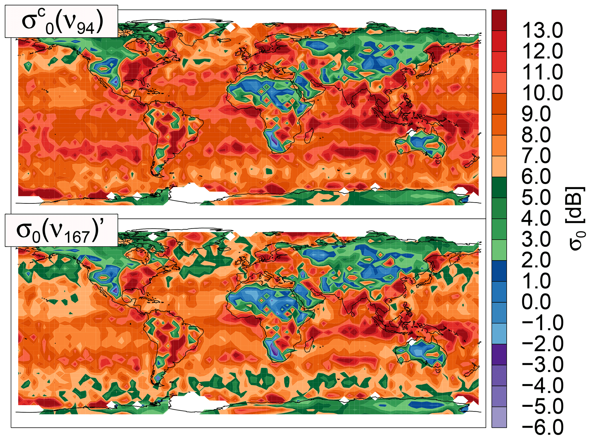
Figure 3Mean CloudSat surface-normalized backscattering cross section for 1–8 January 2007 () and modified backscattering cross section at 167 GHz (σ0(ν167)′). Note that we are displaying the log of the average.
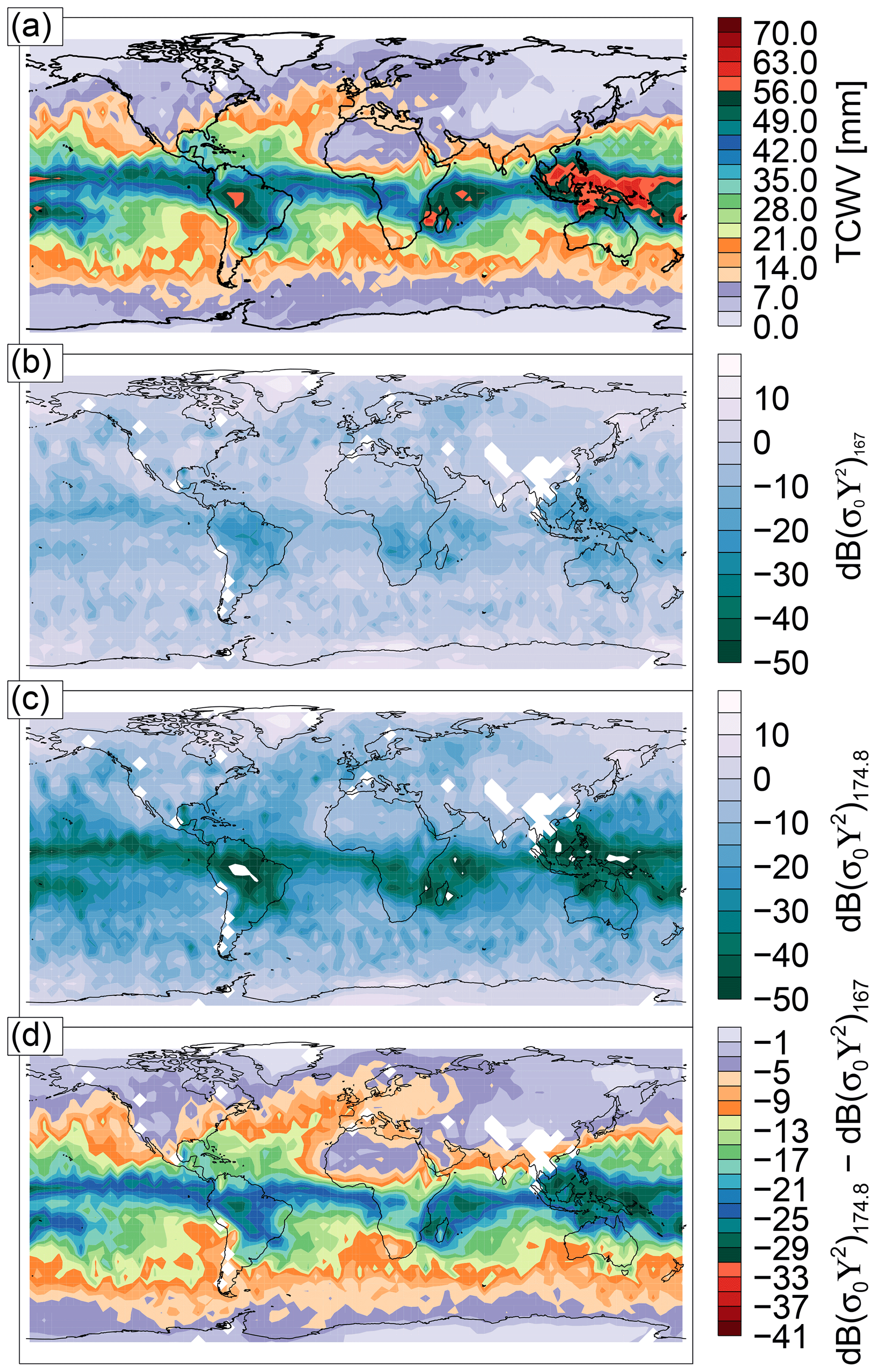
Figure 4Maps exemplifying the CloudSat-driven simulation burdens (1–8 January 2007). (a) Total column water vapor, (b) simulated CloudSat-driven effective surface cross section at 167 GHz, (c) simulated CloudSat-driven effective surface cross section at 174.8 GHz, and (d) effective surface cross-sectional difference (174.8–167 GHz). Grid boxes are 4∘ longitude by 4∘ latitude.
Figure 4 shows maps of the DAR simulations used in this study. Panel a is an 8 d average (1–8 January 2007) of the CloudSat ECMWF-aux total column water vapor to show the context of the simulations. Panels b and c show the average effective surface cross section, that is, σ0(ν)Υ(ν)2, at 167 and 174.8 GHz. Lastly, the bottom panel shows the difference between the 174.8 and 167 GHz simulations. Note that the simulations also include the hydrometeor burden, that is, the IWC, LWC, rain, and snow found on each CloudSat profile, which in principle is frequency-dependent. In these maps there are around 80 000 simulations (we only used every 50 CloudSat measurements). These simulations include, according to the CloudSat classification algorithm (Sassen and Wang, 2008), more than 10 000 clouds identified as cirrus and stratocumulus, around 500 as cumulus, 7000 as nimbostratus, and 800 as deep convection. Further, these simulations include around 400 precipitating scenes with rain rates of up to 4.5 mm h−1 according to the rain profile product (L'Ecuyer and Stephens, 2002).
As shown, the impact of the water vapor burden can be seen at both radar tones; however, at 174.8 GHz the radar signal has been considerably more attenuated than at 167 GHz (which is further from the absorption line). Furthermore, the effective cross-sectional difference (174.8–167 GHz), equivalent to the surface radar power ratios, is clearly strongly correlated with the total column water vapor field.
The aims of this study are (1) to quantify the uncertainties in DAR retrievals of total column water vapor and (2) to explore the trade-offs between radar transmit power and sampling of the Earth's real-world meteorological variability. To accomplish this goal we performed end-to-end retrieval simulations. The retrieval algorithm used is
where the total column water vapor, wi, is computed by suitably integrating the vertical water vapor profile xi, and y is determined by the ratios between surface radar returns at different frequencies, that is to say
and the simulated measurements, , are given by
where F is the radar forward model described in Sect. 3 and b is comprised of forward model parameters that influence the simulated radar observations but are not retrieved. For example, these include spectroscopic parameters, profiles of temperature, pressure, ice water content, liquid water content, rain or snow. The assumptions made in b contribute to the systematic errors in the estimates of the total column water vapor. In each iteration, is evaluated by finite differences by perturbing the entire water vapor profile, xi, by 1 %. Lastly, after each iteration xi+1 is computed following
That is, the shape of the assumed water vapor profile does not change during the retrieval: it is simply scaled according to the total column water vapor retrieved.
The estimated precision (the error due to random noise affecting the instrument) in the retrieved total column water vapor, w, is given by
where σy is given by
which is simply the propagation of combining the individual errors of PR(ν2) and PR(ν1).
To perform end-to-end retrievals, we first need to define a set of conditions regarded as truth as well as the radar characteristics. As detailed in Sect. 3, these conditions were taken from CloudSat measurements (IWC, LWC, rain, snow, temperature and pressure), while the radar characteristics are listed in Table 1. With these atmospheric conditions and radar parameters, we compute synthetic radar returns to be used as measurements; that is, the synthetic radar returns are given by
where wT is the true water vapor state as provided by the CloudSat-ECMWF product and where bT represents the rest of the atmospheric state (temperature, pressure, and hydrometeor profiles) also provided by the CloudSat-ECMWF product.
These synthetic radar returns are then run through the retrieval algorithm. For the retrieved profile shape, x0, a water vapor profile taken from a ERA-Interim monthly climatology was used. The iterative procedure stops when is lower than 0.05, which is normally achieved within two iterations.
During these retrievals we assume perfect knowledge of the forward model parameters; that is, the simulated radar returns used during the retrieval are given by
or in other words, the only variable changing between y and is the water vapor burden.
Sensitivity to assumed parameters is estimated using a perturbed set of synthetic radar returns following
where b′ represents the perturbed forward model parameter. Only one of the parameters is perturbed at a time; for instance, when computing the systematic uncertainty related to temperature, only the temperature values are perturbed, while the rest (IWC, LWC, rain, snow, particle size distributions, etc.) are left unperturbed. Then, the retrieved total column water vapors using the perturbed measurements are compared to the retrieved values from an unperturbed run, i.e., using the measurements given by Eq. (18). The difference between the two retrieved total column water vapors is used a measure of the impact of a given systematic error source. Instrument noise is not added to any of these simulations because its impacts are studied through Eq. (16).
First we will explore the precision, that is, the expected random error associated with the radar uncertainty described in Sect. 2. Then we will explore potential systematic errors, such as the impact of not knowing the hydrometeor burden by assuming clear-sky conditions throughout the forward model simulations, the impact of not knowing precisely the temperature and pressure by using climatological values, the impact of changing the initial assumed water vapor profile, the impact of the spectroscopy errors, and surface roughness uncertainties by using a constant value.
5.1 Precision
Figure 5, left, shows maps of the total column water vapor precision (random error) assuming different transmit powers. White areas denote regions with no CloudSat measurements to initialize the simulations (i.e., the poles) or regions where the pulses (the simulated PRs used in y) are attenuated beneath the noise floor (i.e., the tropics when using 0.1 W of transmit power). As shown even with just a transmit power of 0.1 W, errors are better than 1.2 mm throughout the globe except at the tropics, where the radar tones are completely attenuated. With a transmit power greater than 20 W errors are mostly below 1.2 mm everywhere except in active deep convective regions such as the maritime continent. Further increasing the transmit power does little to improve the precision, because as we noted in Sect. 2, in high SNR regimes, the fractional error in the measurement is largely determined by the number of uncorrelated pulses used. Figure 6 shows the cumulative SNR histogram for the 174.8 GHz surface returns. As can be seen, most of the time, the SNR is higher than 10 even when using just 0.1 W. The SNR for the 167 GHz radar tone is slightly better since it experiences less water vapor attenuation.
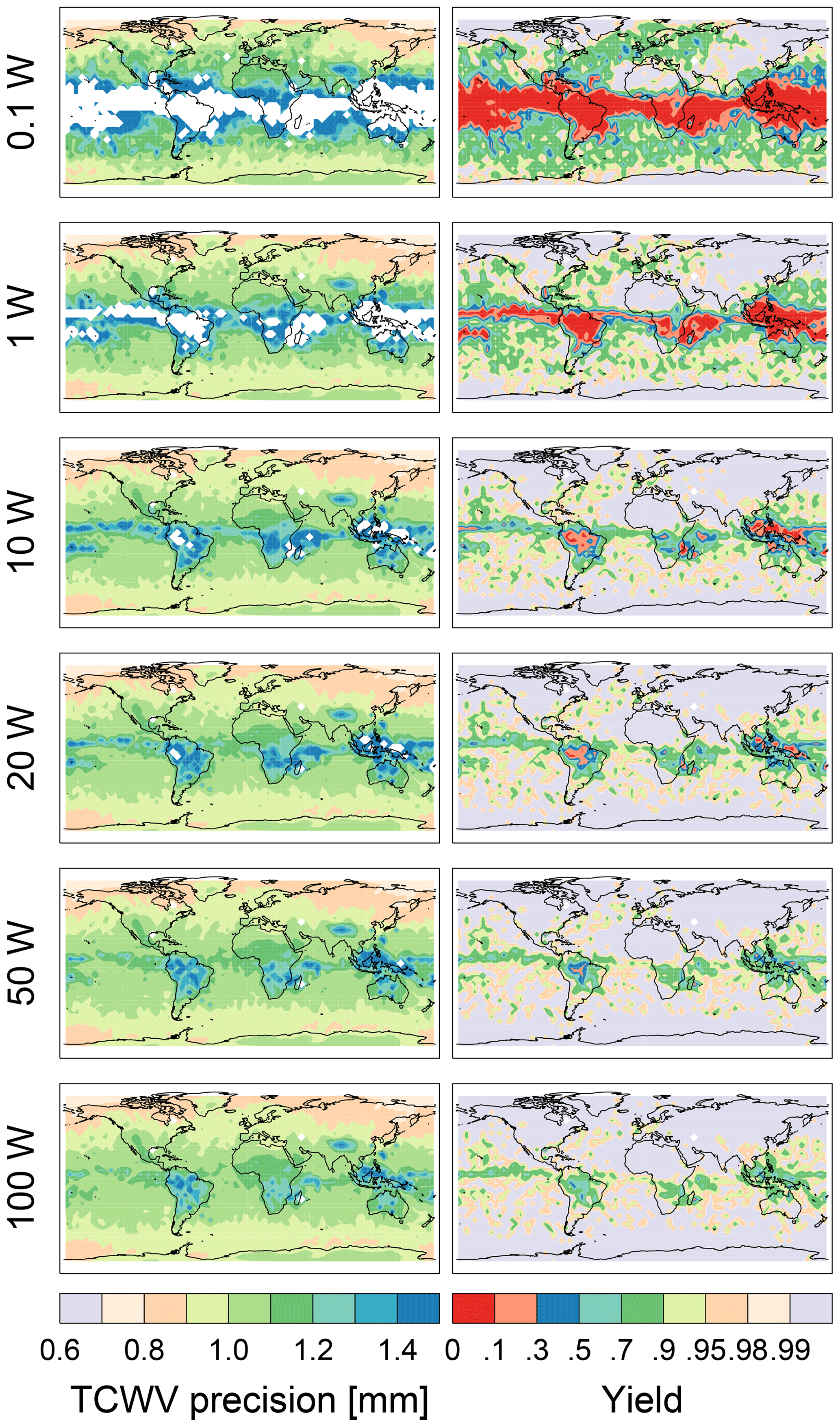
Figure 5Total column water vapor (TCWV) precision maps as well as fractional yield maps for different transmit powers.
Instead, increasing the transmit power improves the yield, that is, the number of times surface reflections at both frequencies are detected with a SNR greater than 1 divided by the total number of simulations. Figure 5, right, shows fractional yield maps for the same transmit powers as those shown in the left panels. Overall, even with only 0.1 W transmit power, the yield is better than 0.7 throughout most of the globe except at the tropics, where the yield sharply drops to zero. The yield improves drastically when using at least 10 W.
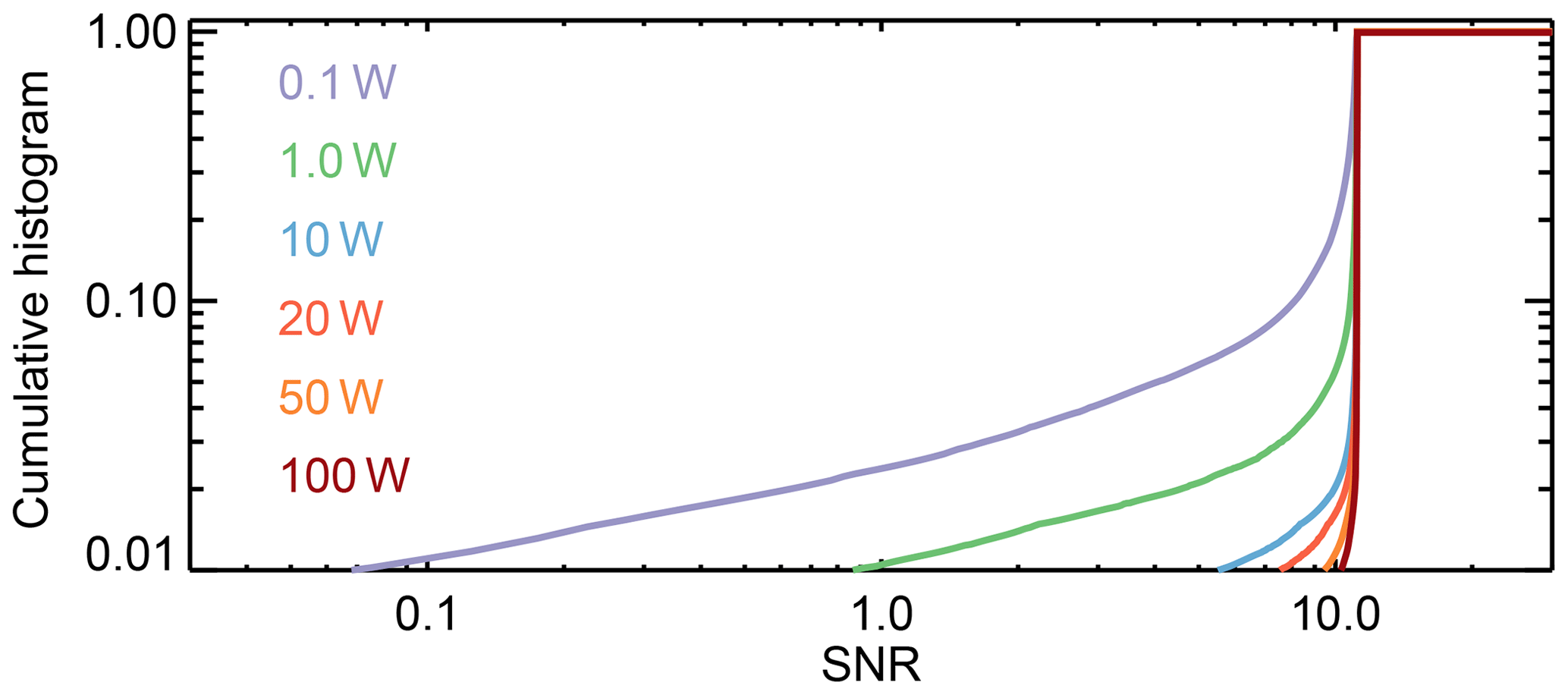
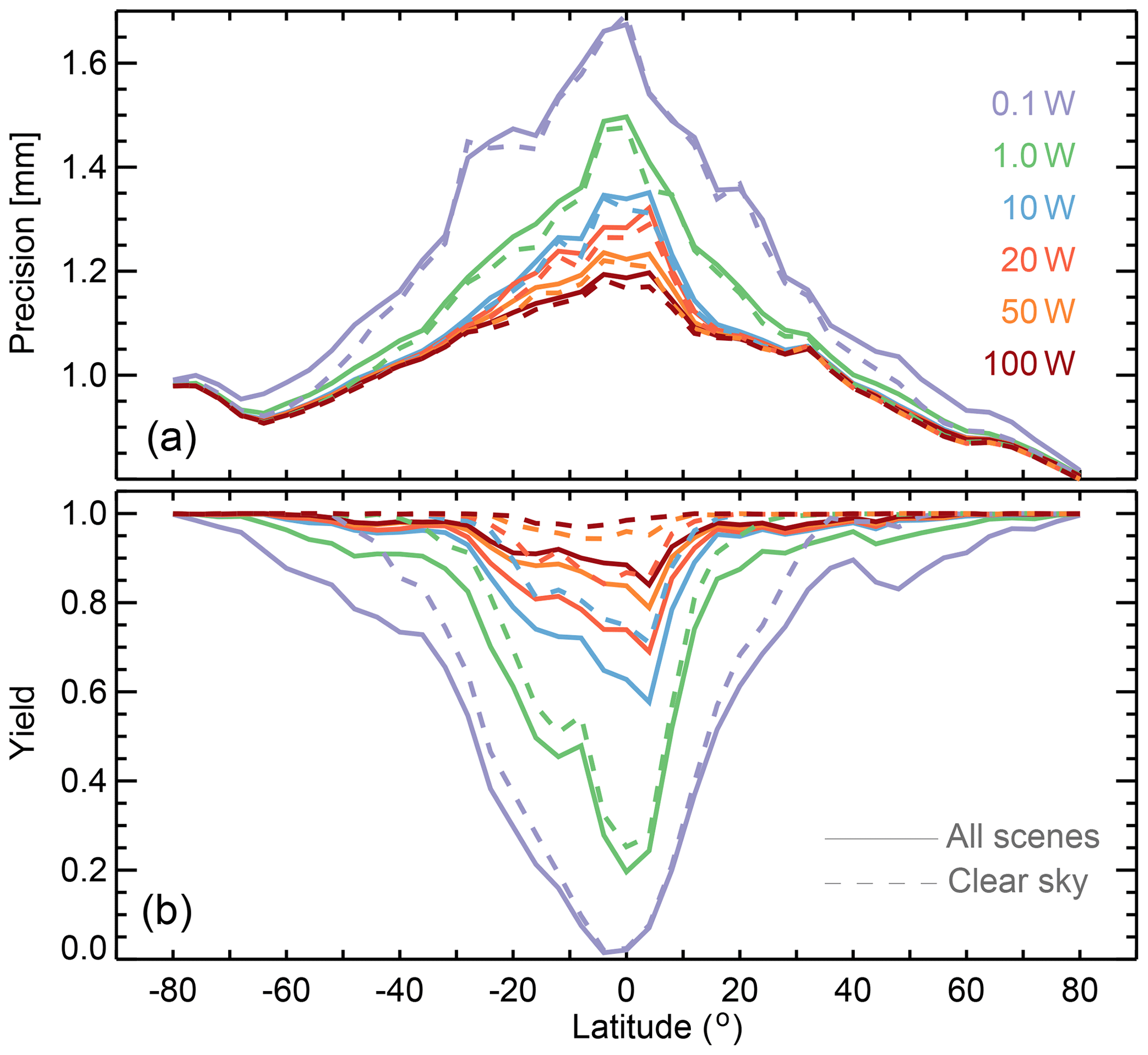
Figure 7Total column water vapor precision (a) as well as fractional yield (b) for different transmit powers vs. latitude.
To complement these maps, Fig. 7 shows the random errors and the fractional yield zonal averages. Outside the tropics, that is, polewards of 30∘ S or 30∘ N, regardless of transmit power, random errors are generally below 1.2 mm with fractional yields better than 0.7. With a transmit power of at least 10 W the random errors are below 1 mm and the fractional yield improves to better than 0.9. In the tropics, using at least 20 W, the random errors are mostly below 1.3 mm with fractional yields better than 0.7, improving to random errors mostly below 1.2 mm with fractional yields better than 0.8 when using at least 50 W. Under clear-sky conditions, the random errors remain mostly the same. The yield, however, improves substantially. For example, in the tropics, for 20 W of transmit power, the yields become better than 0.85 (as opposed to better than 0.7), and for 50 W they become better than 0.95 (as opposed to better than 0.8). This yield improvement under clear-sky cases is due to the lack of the attenuation burden imposed by hydrometeors.
To further highlight that this technique will work under cloudy and precipitating conditions, Fig. 8 shows a cross section of CloudSat-driven simulations over the Southern Ocean. This cross section consists of 500 CloudSat profiles encompassing ice clouds, liquid clouds, rain, and snow. Yields in this cross section are similar to those shown in Fig. 7 at around 55∘ S for the all scenes zonal average yield.
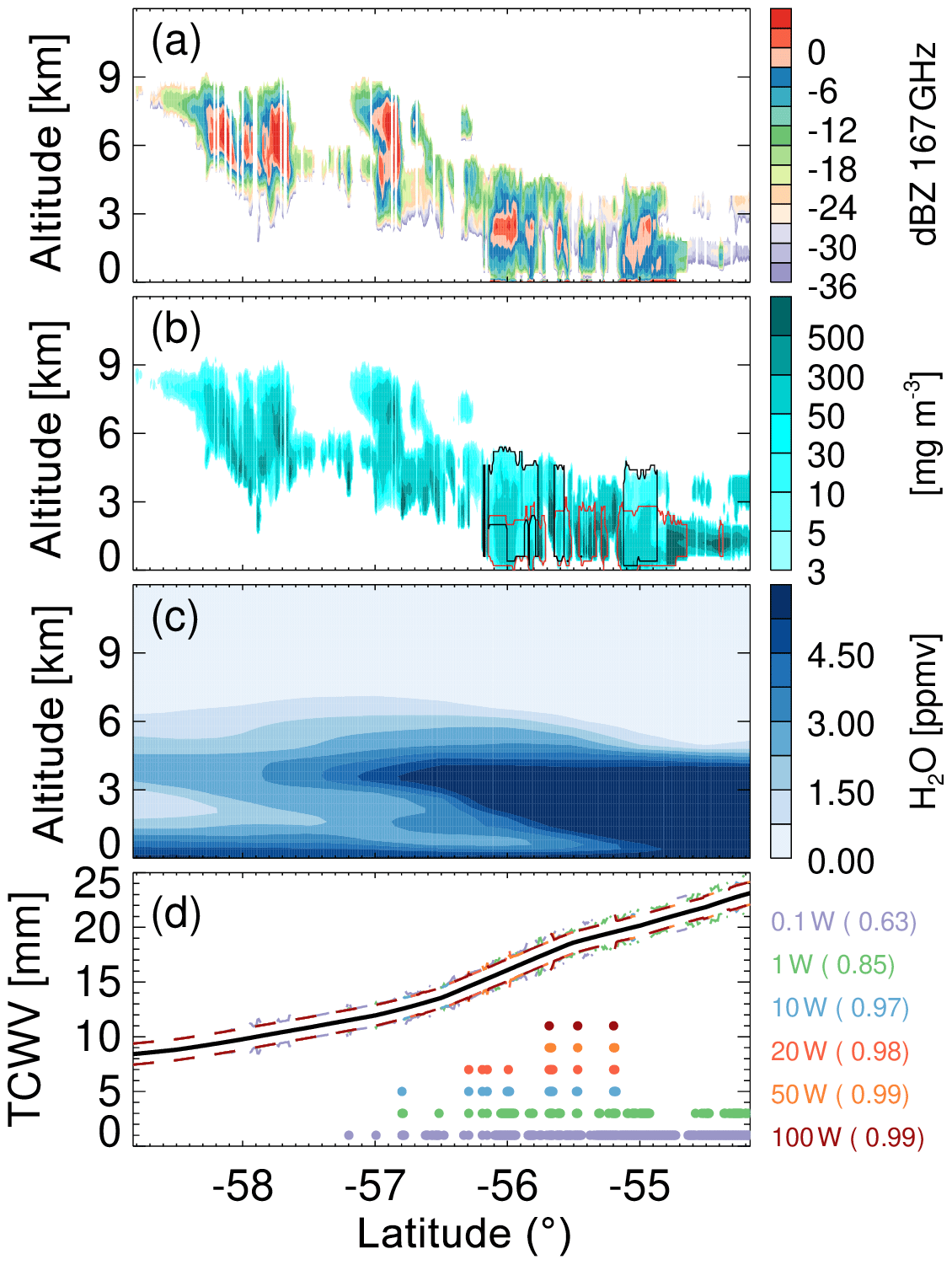
Figure 8Cross section exemplifying the CloudSat-driven simulations (data from 1 January 2007 over the Southern Ocean). (a) Simulated CloudSat-driven radar reflectivity at 167 GHz. (b) CloudSat-retrieved total (IWC+LWC+rain+snow) hydrometeor water content. Black and red lines delimit areas where snow and rain were detected. (c) ECMWF-aux water vapor. (d) Total column water vapor (black solid line) as well as the retrieval precision (dashed lines) for different transmit powers and locations (dots) where at least one of the radar pulses was attenuated beneath the noise floor. Yield values for each simulated transmit powers are given by the numbers in brackets.
To date, passive microwave instruments have provided the benchmark for total column water vapor measurements. For example, the Advanced Microwave Scanning Radiometer (AMSR) instruments have an estimated error of ∼0.6 mm (Wentz and Meissner, 2000) for a native footprint of around 14 km by 8 km (Kawanishi et al., 2003). The precision of aggregated DAR total column water vapor measurements (the ones simulated here) matching such a footprint would be considerably better.
5.2 Systematic uncertainties
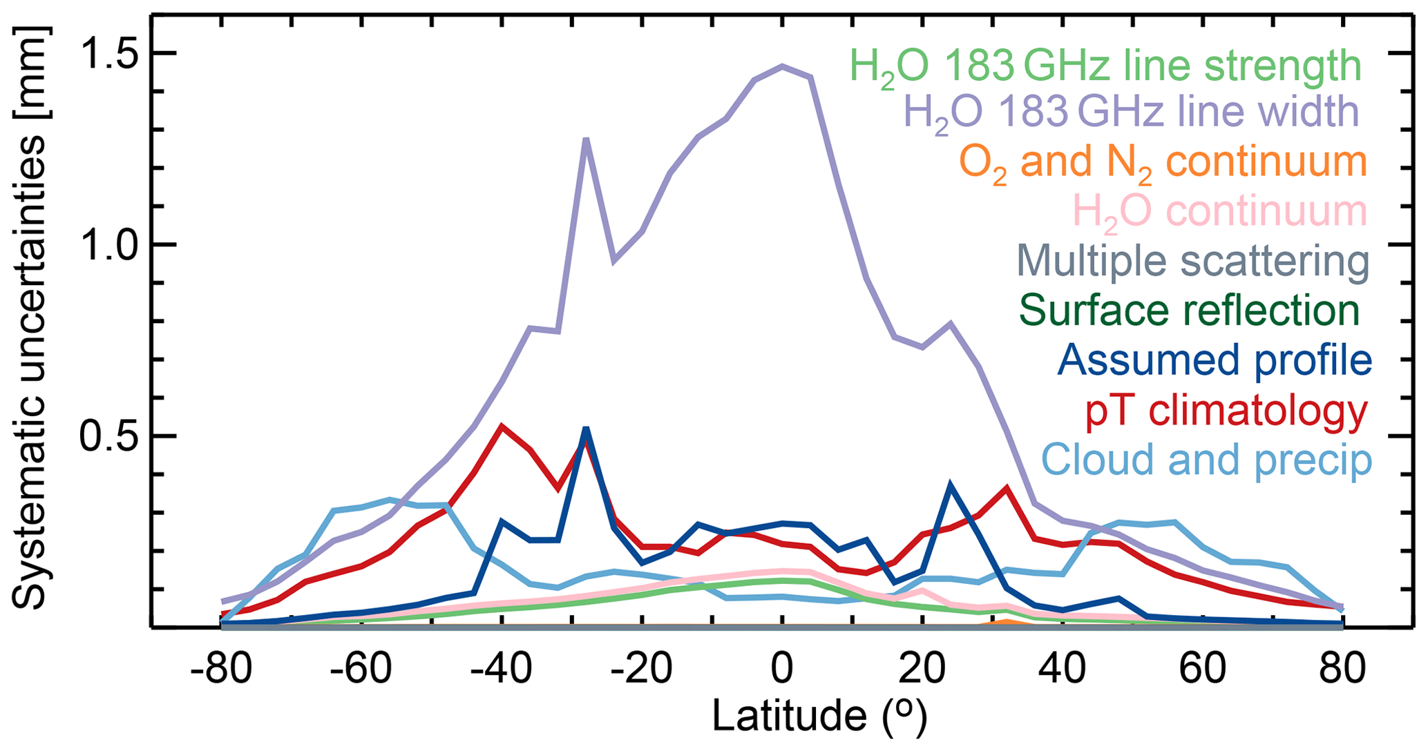
Figure 9 shows zonal averages of eight potential systematic uncertainty sources. As explained in Sect. 4, these systematic errors arise from the uncertainties in the ancillary knowledge used (including the spectroscopy uncertainties) throughout the retrievals. For example, as shown by Eq. (5) the uncertainties in the water vapor mass extinction cross section, κ(ν,r), will affect the estimated total column water vapor. Note that these systematic errors are independent of the transmit power as long as the surface return is not completely attenuated by the atmosphere. As such, these simulations were performed using 100 W to evaluate them under most conditions; that is, we use 100 W because it has the better yield. The systematic error sources studied here are explained below.
-
pT (pressure–temperature) climatology: errors associated with using climatological pressure and temperature conditions throughout the forward model end-to-end simulated retrievals as opposed to using the actual pressure and temperature conditions. The climatological values correspond to January 2007 ERA-Interim monthly mean values for the 12:00 UT synoptic time. Simply, these errors represent the worst possible impact of not knowing precisely the temperature and pressure.
-
Cloud and precipitation errors: errors associated with assuming clear-sky conditions throughout the end-to-end retrieval simulations as opposed to using the actual hydrometeor conditions, in other words, having no hydrometeor information to constrain the retrievals. Note that these error estimates represent the additional frequency-dependent attenuation imposed by the hydrometeors. That is, it is assumed that the radar system is capable of identifying the surface return through coarse ranging capability.
-
Assumed water vapor profile: errors associated with using a different linearization water vapor profile in the end-to-end simulated retrievals. The assumed profiles are perturbed by up to 20 % by layers. That is, we perturb the profile between 0–2, 2–4, 4–6, and 6–8 km individually and then aggregate the systematic uncertainty.
-
Multiple scattering: errors associated with simulating single scattering returns as opposed to multiple scattering ones.
-
H2O 183 GHz line strength: error associated with perturbing the 183 GHz water vapor line strength by 0.25 % following the uncertainty described by Pickett et al. (1998).
-
H2O 183 GHz line width: error associated with perturbing the 183 GHz water vapor line width by 4 % following Bauer et al. (1989) and Goyette and Lucia (1990).
-
H2O continuum: error associated with perturbing the H2O continuum by 10 % following Meshkov and De Lucia (2005).
-
O2 and N2 continuum: errors associated with perturbing the O2 and N2O continuum by 10 % following Meshkov and De Lucia (2005).
-
Surface roughness: errors associated with using a constant 12 ms−1 as opposed to a surface wind climatology.
As shown in Fig. 9, all the potential systematic uncertainties are lower than 0.5 mm, including those uncertainties accounting for the extra attenuation imposed by clouds and precipitation (as long as they do not attenuate completely the radar pulses). The exceptions are the errors associated with the H2O 183 GHz line width, which could be as big as 1.4 mm. As expected, this uncertainty is approximately 4 % of the total column water vapor because a H2O line width perturbation mostly equates to perturbing the measurement, that is, the ratio of the surface radar returns at different frequencies, by the same amount. However, this type of bias should be easily corrected during a validation campaign since all retrievals will be off by the same constant amount.
In all scenarios simulated here, the surface return dwarfed the multiple-scattered component of clouds and rain. That is, the systematic uncertainty induced by ignoring multiple scattering effects was negligible, because the screening of the precipitating scenes (disregarding profiles which had any negative values) screened out those scenarios where multiple scattering was present. However, we do not anticipate that multiple scattering will be a problem, because according to Battaglia et al. (2008), 80 % of the rainy profiles can be accurately modeled assuming a single scattering approximation, and, further, on the order of 20 % of the cases, the strong hydrometeor burden will presumably hinder the surface return.
We have evaluated the precision, yield, and systematic uncertainties of a differential absorption radar to measure total column water vapor from space. This technique requires at least two radar tones near the 183 GHz water vapor absorption line (“on” and “off” the line) to infer the humidity burden between the radar and the surface. In this work, we used 167 and 174.8 GHz, the extremes of the frequency range of VIPR (Roy et al., 2019). Further, we assume an antenna diameter of 1 m, a horizontal integration of 500 m, an integration time of 33 ms, a system temperature of 1800 K, an orbit of 405 km, and transmit powers varying from 0.1 to 100 W.
We apply a radar instrument simulator to weather analysis fields colocated with CloudSat near-global measurements to simulate surface radar returns to be used as measurements in end-to-end retrievals. We use an iterative least-squares fit retrieval algorithm that allows us to quantify both the expected precision and the impact of potential systematic uncertainties upon the retrieved total column water vapor.
Systematic uncertainties related to the pressure and temperature, the hydrometeor burden, the initial guess, the water vapor line strength, the water vapor, O2 and N2 continuum, multiple scattering effects, and the magnitude of the surface winds could result in potential biases lower than 0.5 mm. Systematic uncertainties associated with the water vapor line width could be up to 1.4 mm. This approximately corresponds to 4 % of the total column water vapor because a H2O line width perturbation mostly equates to perturbing the ratio of the surface radar returns by the same amount.
Precision and yield results can be summarized as follows.
-
Outside the tropics, regardless of transmit power, random errors are generally below 1.2 mm with fractional yields better than 0.7. With a transmit power of at least 10 W the random errors are below 1 mm and the fractional yield improves to better than 0.9.
-
In the tropics, using at least 20 W, the random errors are mostly below 1.3 mm with fractional yields better than 0.7, improving to mostly below 1.2 mm with fractional yields better than 0.8 when using at least 50 W.
These results suggest that at least 20 W of transmit power are needed to be able to measure total column water vapor globally with a reasonable yield. Output powers in the 10–100 W range would require additional research and development. DAR holds considerable potential as a technique to study the distribution of total column water vapor globally, that is, under most terrains and under most meteorological conditions, with considerably high horizontal resolution.
The CloudSat dataset used in this paper can be found on the CloudSat data processing center website (http://www.cloudsat.cira.colostate.edu/order-data, last access: 1 March 2020; CloudSat DPC, 2020).
LM wrote the algorithm and carried out the analyses. RR and ML provided scientific expertise throughout all stages of the research.
The authors declare that they have no conflict of interest.
The research was carried out at the Jet Propulsion Laboratory, California Institute of Technology, under a contract with the National Aeronautics and Space Administration. We thank Ken Cooper for his support throughout this research.
This paper was edited by Murray Hamilton and reviewed by two anonymous referees.
Abel, S. J. and Boutle, I. A.: An improved representation of the raindrop size distribution for single-moment microphysics schemes, Q. J. Roy. Meteor. Soc., 138, 2151–2162, https://doi.org/10.1002/qj.1949, 2012. a
Austin, R. T. and Stephens, G. L.: Retrieval of stratus cloud microphysical parameters using millimeter-wave radar and visible optical depth in preparation for CloudSat: 1. Algorithm formulation, J. Geophys. Res.-Atmos., 106, 28233–28242, https://doi.org/10.1029/2000JD000293, 2001. a
Austin, R. T., Heymsfield, A. J., and Stephens, G. L.: Retrieval of ice cloud microphysical parameters using the CloudSat millimeter-wave radar and temperature, J. Geophys. Res.-Atmos., 114, d00A23, https://doi.org/10.1029/2008JD010049, 2009. a
Battaglia, A. and Kollias, P.: Evaluation of differential absorption radars in the 183 GHz band for profiling water vapour in ice clouds, Atmos. Meas. Tech., 12, 3335–3349, https://doi.org/10.5194/amt-12-3335-2019, 2019. a
Battaglia, A., Haynes, J. M., L'Ecuyer, T., and Simmer, C.: Identifying multiple-scattering-affected profiles in CloudSat observations over the oceans, J. Geophys. Res., 113, D00A17, https://doi.org/10.1029/2008jd009960, 2008. a
Bauer, A., Godon, M., Kheddar, M., and Hartmann, J.: Temperature and perturber dependences of water vapor line-broadening. Experiments at 183 GHz; calculations below 1000 GHz, J. Quant. Spectrosc. Ra., 41, 49–54, https://doi.org/10.1016/0022-4073(89)90020-4, 1989. a
Bedka, S., Knuteson, R., Revercomb, H., Tobin, D., and Turner, D.: An assessment of the absolute accuracy of the Atmospheric Infrared Sounder v5 precipitable water vapor product at tropical, midlatitude, and arctic ground-truth sites: September 2002 through August 2008, J. Geophys. Res., 115, D17310, https://doi.org/10.1029/2009jd013139, 2010. a
Browell, E. V., Wilkerson, T. D., and Mcilrath, T. J.: Water vapor differential absorption lidar development and evaluation, Appl. Optics, 18, 3474–3483, https://doi.org/10.1364/AO.18.003474, 1979. a
CloudSat DPC: CloudSat Data Processing Center, 2C-RAINPROFILE. 2B-CWCRO R05, ECMWF-aux, available at: http://www.cloudsat.cira.colostate.edu/order-data, last access: 1 March 2020. a
Cooper, K. B., Monje, R. R., Millán, L., Lebsock, M., Tanelli, S., Siles, J. V., Lee, C., and Brown, A.: Atmospheric Humidity Sounding Using Differential Absorption Radar Near 183 GHz, IEEE Geosci. Remote S., 15, 163–167, https://doi.org/10.1109/lgrs.2017.2776078, 2018. a
Cronk, H. and Partain, P.: CloudSat ECMWF-AUX Auxillary Data Product Process Description and Interface Control Document, Product Version: P_R05, available at: http://www.cloudsat.cira.colostate.edu/sites/default/files/products/files/ECMWF-AUX_PDICD.P_R05.rev0_.pdf (last access: 1 March 2020), 2017. a
Dee, D. P., Uppala, S. M., Simmons, A. J., Berrisford, P., Poli, P., Kobayashi, S., Andrae, U., Balmaseda, M. A., Balsamo, G., Bauer, P., Bechtold, P., Beljaars, A. C. M., van de Berg, L., Bidlot, J., Bormann, N., Delsol, C., Dragani, R., Fuentes, M., Geer, A. J., Haimberger, L., Healy, S. B., Hersbach, H., Hólm, E. V., Isaksen, L., Kållberg, P., Köhler, M., Matricardi, M., McNally, A. P., Monge-Sanz, B. M., Morcrette, J.-J., Park, B.-K., Peubey, C., de Rosnay, P., Tavolato, C., Thépaut, J.-N., and Vitart, F.: The ERA-Interim reanalysis: configuration and performance of the data assimilation system, Q. J. Roy. Meteor. Soc., 137, 553–597, https://doi.org/10.1002/qj.828, 2011. a
Diedrich, H., Preusker, R., Lindstrot, R., and Fischer, J.: Retrieval of daytime total columnar water vapour from MODIS measurements over land surfaces, Atmos. Meas. Tech., 8, 823–836, https://doi.org/10.5194/amt-8-823-2015, 2015. a
Ellis, S. M. and Vivekanandan, J.: Water vapor estimates using simultaneous dual-wavelength radar observations, Radio Sci., 45, RS5002, https://doi.org/10.1029/2009rs004280, 2010. a
GCOS-ECV: Global Climate Observing System – Essential Climate Variable, available at: https://www.ncdc.noaa.gov/gosic/gcos-essential-climate-variable-ecv-data-access-matrix/gcos-atmosphere-upper-air-ecv-water-vapour, last access: 11 March 2020. a
Goyette, T. M. and Lucia, F. C. D.: The pressure broadening of the 31, 3-22, 0 transition of water between 80 and 600 K, J. Mol. Spectrosc., 143, 346–358, https://doi.org/10.1016/0022-2852(91)90099-v, 1990. a
Haynes, J. M., L'Ecuyer, T. S., Stephens, G. L., Miller, S. D., Mitrescu, C., Wood, N. B., and Tanelli, S.: Rainfall retrieval over the ocean with spaceborne W-band radar, J. Geophys. Res., 114, D00A22, https://doi.org/10.1029/2008jd009973, 2009. a
Hogan, R. J.: Multiscatter: a fast, approximate multiple scattering algorithm, University of Reading, Reading, UK, 2013. a
Hogan, R. J. and Battaglia, A.: Fast Lidar and Radar Multiple-Scattering Models. Part II: Wide-Angle Scattering Using the Time-Dependent Two-Stream Approximation, J. Atmos. Sci., 65, 3636–3651, https://doi.org/10.1175/2008jas2643.1, 2008. a, b
Hufford, G.: A model for the complex permittivity of ice at frequencies below 1 THz, Int. J. Infrared Milli., 12, 677–682, https://doi.org/10.1007/bf01008898, 1991. a
Kawanishi, T., Sezai, T., Ito, Y., Imaoka, K., Takeshima, T., Ishido, Y., Shibata, A., Miura, M., Inahata, H., and Spencer, R.: The advanced microwave scanning radiometer for the earth observing system (AMSR-E), NASDA's contribution to the EOS for global energy and water cycle studies, IEEE T. Geosci. Remote, 41, 184–194, https://doi.org/10.1109/tgrs.2002.808331, 2003. a
Lang, R., Casadio, S., Maurellis, A. N., and Lawrence, M. G.: Evaluation of the GOME Water Vapor Climatology 1995–2002, J. Geophys. Res., 112, D17110, https://doi.org/10.1029/2006jd008246, 2007. a
Lebsock, M. D. and L'Ecuyer, T. S.: The retrieval of warm rain from CloudSat, J. Geophys. Res.-Atmos., 116, d20209, https://doi.org/10.1029/2011JD016076, 2011. a
Lebsock, M. D., Suzuki, K., Millán, L. F., and Kalmus, P. M.: The feasibility of water vapor sounding of the cloudy boundary layer using a differential absorption radar technique, Atmos. Meas. Tech., 8, 3631–3645, https://doi.org/10.5194/amt-8-3631-2015, 2015. a, b, c
L'Ecuyer, T. S. and Stephens, G. L.: An Estimation-Based Precipitation Retrieval Algorithm for Attenuating Radars, J. Appl. Meteorol., 41, 272–285, https://doi.org/10.1175/1520-0450(2002)041<0272:aebpra>2.0.co;2, 2002. a
Li, L., Heymsfield, G. M., Tian, L., and Racette, P. E.: Measurements of Ocean Surface Backscattering Using an Airborne 94-GHz Cloud Radar Implication for Calibration of Airborne and Spaceborne W-Band Radars, J. Atmos. Ocean. Tech., 22, 1033–1045, https://doi.org/10.1175/jtech1722.1, 2005. a, b, c, d
Liebe, H. J., Hufford, G. A., and Manabe, T.: A model for the complex permittivity of water at frequencies below 1 THz, Int. J. Infrared Milli., 12, 659–675, https://doi.org/10.1007/BF01008897, 1991. a
Lindstrot, R., Preusker, R., Diedrich, H., Doppler, L., Bennartz, R., and Fischer, J.: 1D-Var retrieval of daytime total columnar water vapour from MERIS measurements, Atmos. Meas. Tech., 5, 631–646, https://doi.org/10.5194/amt-5-631-2012, 2012. a
McFarquhar, G. M. and Heymsfield, A. J.: Parameterization of Tropical Cirrus Ice Crystal Size Distributions and Implications for Radiative Transfer: Results from CEPEX, J. Atmos. Sci., 54, 2187–2200, https://doi.org/10.1175/1520-0469(1997)054<2187:POTCIC>2.0.CO;2, 1997. a
Meneghini, R., Liao, L., and Tian, L.: A Feasibility Study for Simultaneous Estimates of Water Vapor and Precipitation Parameters Using a Three-Frequency Radar, J. Appl. Meteorol., 44, 1511–1525, https://doi.org/10.1175/jam2302.1, 2005. a
Meshkov, A. I. and De Lucia, F. C.: Broadband absolute absorption measurements of atmospheric continua with millimeter wave cavity ringdown spectroscopy, Rev. Sci. Instrum., 76, 083103, https://doi.org/10.1063/1.1988027, 2005. a, b
Millán, L., Lebsock, M., Livesey, N., Tanelli, S., and Stephens, G.: Differential absorption radar techniques: surface pressure, Atmos. Meas. Tech., 7, 3959–3970, https://doi.org/10.5194/amt-7-3959-2014, 2014. a
Millán, L., Lebsock, M., Livesey, N., and Tanelli, S.: Differential absorption radar techniques: water vapor retrievals, Atmos. Meas. Tech., 9, 2633–2646, https://doi.org/10.5194/amt-9-2633-2016, 2016. a, b, c, d
Nelson, R. R., Crisp, D., Ott, L. E., and O'Dell, C. W.: High-accuracy measurements of total column water vapor from the Orbiting Carbon Observatory-2, Geophys. Res. Lett., 43, 12261–12269, https://doi.org/10.1002/2016GL071200, 2016. a
NTIA: National Telecommunications and Information Administration: Manual of Regulations and Procedures for Federal Radio Frequency Management, available at: https://www.ntia.doc.gov/page/2011/ (last access: 3 March 2020), 2015. a
Pearson, J. C., Cooper, K., and Drouin, B. J.: Spectroscopic detection, fundamental limits and system considerations, in: 2008 33rd International Conference on Infrared, Millimeter and Terahertz Waves, IEEE, https://doi.org/10.1109/icimw.2008.4665839, 2008. a
Peral, E., Tanelli, S., Statham, S., Joshi, S., Imken, T., Price, D., Sauder, J., Chahat, N., and Williams, A.: RainCube: the first ever radar measurements from a CubeSat in space, J. Appl. Remote Sens., 13, 1, https://doi.org/10.1117/1.jrs.13.032504, 2019. a
Pickett, H., Poynter, R., Cohen, E., Delitsky, M., Pearson, J., and Müller, H.: SUBMILLIMETER, MILLIMETER, AND MICROWAVE SPECTRAL LINE CATALOG, J. Quant. Spectrosc. Ra., 60, 883–890, https://doi.org/10.1016/s0022-4073(98)00091-0, 1998. a
Pougatchev, N., August, T., Calbet, X., Hultberg, T., Oduleye, O., Schlüssel, P., Stiller, B., Germain, K. St., and Bingham, G.: IASI temperature and water vapor retrievals – error assessment and validation, Atmos. Chem. Phys., 9, 6453–6458, https://doi.org/10.5194/acp-9-6453-2009, 2009. a
Read, W. G., Shippony, Z., and Snyder, W. V.: EOS MLS Forward Model Algorithm Theoretical Basis Document, Jet Propulsion Lab., JPL D-18130CL#04-2238, Pasadena, CA, USA, 2004. a, b
Roy, R. J., Lebsock, M., Millán, L., and Cooper, K. B.: Validation of a G-Band Differential Absorption Cloud Radar for Humidity Remote Sensing. J. Atmos. Ocean. Technol., 37, 1085–1102, https://doi.org/10.1175/JTECH-D-19-0122.1, 2020. a, b, c
Roy, R. J., Lebsock, M., Millán, L., Dengler, R., Rodriguez Monje, R., Siles, J. V., and Cooper, K. B.: Boundary-layer water vapor profiling using differential absorption radar, Atmos. Meas. Tech., 11, 6511–6523, https://doi.org/10.5194/amt-11-6511-2018, 2018. a, b
Sassen, K. and Wang, Z.: Classifying clouds around the globe with the CloudSat radar: 1-year of results, Geophys. Res. Lett., 35, L04805, https://doi.org/10.1029/2007gl032591, 2008. a
Schluessel, P. and Emery, W. J.: Atmospheric water vapour over oceans from SSM/I measurements, Int. J. Remote Sens., 11, 753–766, https://doi.org/10.1080/01431169008955055, 1990. a
Schotland, R. M.: Some observations of the vertical profile of water vapor by means of a ground based optical radar, Proceedings of the Fourth Symposium on Remote Sensing of the Environment, Environmental Research Institute of Michigan, Ann Arbor, MI, USA, 273–283, 1966. a
Sekhon, R. S. and Sirvastava, R. C.: Snow size spectra and radar reflectivity,, J. Atmos. Sci., 37, 299–370, https://doi.org/10.1175/1520-0469(1970)027<0299:SSSARR>2.0.CO;2, 1970. a
Stephens, G. L., Vane, D. G., Boain, R. J., Mace, G. G., Sassen, K., Wang, Z., Illingworth, A. J., O'Connor, E. J., Rossow, W. B., Durden, S. L., Miller, S. D., Austin, R. T., Benedetti, A., Mitrescu, C., and Team, T. C. S.: THE CLOUDSAT MISSION AND THE A-TRAIN: A New Dimension of Space-Based Observations of Clouds and Precipitation, B. Am. Meteorol. Soc., 83, 1771–1790, https://doi.org/10.1175/bams-83-12-1771, 2002. a, b
Tian, L., Heymsfield, G. M., Li, L., and Srivastava, R. C.: Properties of light stratiform rain derived from 10- and 94-GHz airborne Doppler radars measurements, J. Geophys. Res., 112, D11211, https://doi.org/10.1029/2006jd008144, 2007. a
Townes, C. H. and Geschwind, S.: Limiting Sensitivity of a Microwave Spectrometer, J. Appl. Phys., 19, 795–796, https://doi.org/10.1063/1.1698206, 1948. a
Walsh, E. J.: Pulse-to-pulse correlation in satellite radar altimeters, Radio Sci., 17, 786–800, https://doi.org/10.1029/rs017i004p00786, 1982. a
Wang, H., Liu, X., Chance, K., González Abad, G., and Chan Miller, C.: Water vapor retrieval from OMI visible spectra, Atmos. Meas. Tech., 7, 1901–1913, https://doi.org/10.5194/amt-7-1901-2014, 2014. a
Wentz, F. J.: A well-calibrated ocean algorithm for special sensor microwave/imager, J. Geophys. Res.-Oceans, 102, 8703–8718, https://doi.org/10.1029/96jc01751, 1997. a
Wentz, F. J. and Meissner, T.: AMSR ocean algorithm, version 2, Remote Sensing Systems Tech. Rep. 121599A-1, 66 pp., available at: http://eospso.gsfc.nasa.gov/sites/default/files/atbd/atbd-amsr-ocean.pdf (last access: 1 March 2020), 2000. a
Wulfmeyer, V. and Walther, C.: Future performance of ground-based and airborne water-vapor differential absorption lidar. II. Simulations of the precision of a near-infrared, high-power system, Appl. Opt., 40, 5321–5336, https://doi.org/10.1364/AO.40.005321, 2001. a