Evaluation of UV aerosol retrievals from an ozone lidar

Aerosol retrieval using ozone lidars in the ultraviolet spectral region is challenging but necessary for correcting aerosol interference in ozone retrieval and for studying the ozone–aerosol correlations. This study describes the aerosol retrieval algorithm for a tropospheric ozone lidar, quantifies the retrieval error budget, and intercompares the aerosol retrieval products at 299 nm with those at 532 nm from a high spectral resolution lidar (HSRL) and with those at 340 nm from an AErosol RObotic NETwork radiometer. After the cloud-contaminated data are filtered out, the aerosol backscatter or extinction coefficients at 30 m and 10 min resolutions retrieved by the ozone lidar are highly correlated with the HSRL products, with a coefficient of 0.95 suggesting that the ozone lidar can reliably measure aerosol structures with high spatiotemporal resolution when the signal-to-noise ratio is sufficient. The actual uncertainties of the aerosol retrieval from the ozone lidar generally agree with our theoretical analysis. The backscatter color ratio (backscatter-related exponent of wavelength dependence) linking the coincident data measured by the two instruments at 299 and 532 nm is 1.34±0.11, while the Ångström (extinction-related) exponent is 1.49±0.16 for a mixture of urban and fire smoke aerosols within the troposphere above Huntsville, AL, USA.

1 Introduction

A tropospheric ozone differential absorption lidar (DIAL) makes measurements of vertical ozone profiles, typically at two wavelengths chosen between 277 and 300 nm with a separation less than 12 nm, by weighing several parameters such as the ozone absorption cross sections, solar background, dynamic range of the detection system, and interference from aerosols and other species (e.g., Alvarez et al., 2011; Browell et al., 1985; De Young et al., 2017; Fukuchi et al., 2001; Kempfer et al., 1994; McDermid et al., 2002; Proffitt and Langford, 1997; Strawbridge et al., 2018; Sullivan et al., 2014). Vertical aerosol profiles are of high interest not only because they are needed for aerosol correction in ozone lidar retrievals (Steinbrecht and Carswell, 1995) but also because simultaneous ozone and aerosol vertical profile measurements provide unique information on their interactions and on sources of pollutant transport (Browell et al., 1994; Langford et al., 2020; Newell et al., 1999). However, there is currently no consensus on the reliability of the aerosol retrievals produced by ozone lidars due to the difficulty of solving the three-component lidar equation and the large variability in aerosol optical properties associated with the multiplicity of aerosol types and size distributions.

The most widely used solution for the elastic single-wavelength aerosol lidar equation is the analytic method developed by Klett (1981). The inversion method then inspired Fernald (1984) to publish a computer algorithm scheme to solve the more general two-component (aerosol and molecular) atmospheric lidar equation. The Klett (1981) inversion requires a priori value for the lidar ratio (i.e., aerosol extinction-to-backscatter ratio, represented by “S” hereafter) to link the aerosol backscatter with its extinction for solving the lidar equation. Lasers used for aerosol lidars are preferred in the visible and infrared bands, typically 532 and 1064 nm for an Nd:YAG laser or 694 nm for ruby laser (Russell et al., 1979), where the ozone absorption is much smaller than molecular and Mie scattering. In the ultraviolet (UV) band for an ozone lidar, the ozone absorption may not be trivial. Some ozone lidars have an aerosol channel available, either independently or sharing receiving optics with the ozone channel (e.g., Browell et al., 1994; De Young et al., 2017; Gronoff et al., 2019; Kovalev and McElroy, 1994; Uchino and Tabata, 1991). For most of the traditional two-wavelength ozone lidars without an aerosol channel, although there has been some discussion about the aerosol retrieval algorithm (e.g., Eisele and Trickl, 2005; Langford et al., 2019; Papayannis et al., 1999; Sullivan et al., 2014), the evaluation of the aerosol retrieval product and its error budget have rarely been addressed. Due to a significant wavelength difference with aerosol lidars, several aspects of the aerosol retrieval using an ozone lidar are worth noting. First, the signal-to-noise ratio (SNR) for ozone lidars decays quicker with altitude due to more significant UV molecular (i.e., Rayleigh) scattering and ozone absorption resulting in a lower retrievable altitude than aerosol lidars. Second, since the molecular and ozone components become more important at UV wavelengths compared to visible and infrared wavelengths, the uncertainties in aerosol retrieval propagated from the calculation of these two components are expected to be larger for ozone lidars than for aerosol lidars. Third, S and the wavelength dependence used for the ozone lidar wavelengths may be different from those used for the longer aerosol lidar wavelengths (Ackermann 1998; Eck et al., 1999).

The primary objectives of this article are to investigate the performance of our aerosol retrieval algorithm and to quantify its error budget for the ozone lidar. The secondary goal is to seek the overall wavelength dependence between the aerosol optical properties measured by the ozone lidar at 299 nm and by a high spectral resolution lidar (HSRL) at 532 nm.

2 Instruments and data processing

2.1 Ozone lidar

The Rocket-city Ozone (O₃) Quality Evaluation in the Troposphere (RO₃QET) lidar is located on the campus of The University of Alabama in Huntsville (UAH) at 34.725^∘ N, 86.645^∘ W at 206 m a.s.l. and is one of the six systems of the Tropospheric Ozone Lidar Network (TOLNet) (http://www-air.larc.nasa.gov/missions/TOLNet, last access: 20 September 2020). This system measures ozone from 0.1 km up to about 12 km during nighttime and up to about 6 km during daytime with a temporal resolution of 2 min. The vertical resolution of the lidar retrievals varies from 150 m in the lower troposphere to 750 m in the upper troposphere in order to keep the measurement uncertainty within ±10 % (Kuang et al., 2013).

The transmitter comprises two Raman-shifted lasers at 289 and 299 nm. Two 30 Hz, 266 nm Nd:YAG lasers pump two 1.8 m Raman cells with mixtures of active gas and buffer gas to generate 289 and 299 nm lasers with an average pulse energy of about 5 mJ. The receiving system consists of three receivers with diameters of 2.5, 10, and 40 cm and four photomultiplier tubes (PMTs) similar to that described by Kuang et al. (2013) except that the solar filters have been replaced by 300 nm short-pass filters for all telescopes. Channels 1, 2, 3, and 4 represent the 2.5 cm, 10 % of the 10 cm, 90% of the 10 cm, and the 40 cm telescope channels, respectively. Since the modification of channel 4 through the addition of narrowband solar filters was not completed before the time period of this study, data from this channel were not used in this work, with the net result that uncertainties for ozone retrievals above 6 km during daytime were often too large due to the strong solar background. Lidar-signal counting was accomplished by four Licel transient recorders (Licel company, Germany) with both analog and photon-counting (PC) modes, with a sampling rate of 40 MHz corresponding to a 3.75 m fundamental resolution. The cloud base height is determined by the following empirical method. Derivatives of the logarithm of the offline analog signal are calculated for a lidar-signal profile, and the first range bin at which the derivative is greater than a certain threshold is considered to be the cloud base height. The threshold is chosen empirically based on the lidar SNR and the vertical resolution. Therefore, lidar data with cloud base lower than 2 km were discarded. The cloud filtering process should be conducted carefully, because an elastic lidar without a polarization channel is not capable of accurately distinguishing aerosols and clouds solely through their backscatter properties. Five 2 min lidar data intervals were combined to give a 10 min lidar-signal integration time to improve the SNR. Further, six of the 3.75 m fundamental bins were integrated for all channels. In addition, dead-time correction (for PC signal only), background correction, analog and PC signal merging, and signal-induced noise correction were performed.

2.2 Aerosol retrieval and uncertainty estimation

The aerosol profiles were retrieved with an iterative DIAL algorithm (Kuang et al., 2011). A brief description of this algorithm is provided in this section, with further details in Appendix A. A first-order Savitzky–Golay differentiation filter with a second-degree polynomial was applied to the logarithm of the signal ratios to compute the first-cut ozone profile. This initial ozone profile was substituted back into the three-component lidar equation to derive the profile of aerosol backscatter coefficients at 299 nm by assuming a constant S of 60 sr and boundary value of the aerosol backscatter coefficient at a far-range reference altitude (about 10 km). During the daytime, the ozone retrieval was limited by the lower SNR of the 289 nm channel, but the 299 nm channel had much better SNR due to lower atmospheric extinction, and it was able to measure aerosol up to higher altitudes. S has high variability as a function of aerosol characteristics, humidity, and wavelength (Ackermann, 1998; Strawbridge et al., 2018; Mishchenko et al., 1997). The S a priori value assumed for this study represents a mix of urban and smoke aerosols during the lidar observations (Ackermann, 1998; Burton et al., 2012; Cattrall et al., 2005; Groß et al., 2013; Müller et al., 2007). The a priori value is application dependent. In the aerosol retrieval uncertainty discussion in Appendix B, we assume a ±20 % uncertainty for S based on an average standard deviation obtained from prior observations (Müller et al., 2007).

Molecular backscatter and extinction profiles were computed from local radiosonde data. Then, the aerosol profile was substituted into the lidar equation again to obtain a stable solution, usually within three iterations. This aerosol profile was further employed to calculate the aerosol correction for ozone retrievals using the first-order Taylor approximation (Browell et al., 1985) by assuming a power-law wavelength dependence for the aerosol extinction and choosing an appropriate Ångström exponent. Since this work focuses only on aerosol retrieval, details of the ozone correction will be described in a future article. Finally, the aerosol profiles derived by the three altitude channels were merged into a single profile in the overlapping altitude zones, i.e., 0.5–1 km for channels 1 and 2 and 1.5–2 km for channels 2 and 3.

The primary uncertainty sources for the aerosol lidar retrievals are the uncertainties in lidar-signal measurement, boundary value assumption for aerosol backscatter coefficient, air density measurement, S a priori value, and ozone profile input. The relative importance of these sources is altitude dependent. In the planetary boundary layer (PBL) where the air is typically turbid, the S uncertainty is dominant, while other sources are minor (only a few percent). The uncertainty of S influences the uncertainty of the aerosol backscatter through a complicated relationship. However, the magnitude of the above two uncertainties can be approximately seen to be close. At the far range (higher than 7 km), the lidar-signal detection noise and inaccurate boundary value assumption are important. Influence from both of the above sources, especially the boundary value, on the aerosol retrieval quickly decreases towards the ground from the far range. In the middle range (PBL top to 7 km), both the air density measurement error and lidar-signal detection noise are essential. Uncertainty due to ozone profile input is relatively unimportant and is only a few percent at most altitudes. Figure B1 presents an example of the aerosol backscatter uncertainty calculated from 10 min nighttime RO₃QET lidar data. The error budget estimate generally justifies the choice of using 6 km as the maximum altitude for the RO₃QET and HSRL comparison since the total uncertainty for the RO₃QET aerosol retrieval could be unacceptably large (i.e., persistently larger than 100 %).

2.3 HSRL

The University of Wisconsin HSRL (Eloranta, 2005) was deployed in Huntsville, AL, from 19 June to 4 November 2013 and operated almost 24 h every day to support the Studies of Emissions and Atmospheric Composition, Clouds and Climate Coupling by Regional Surveys SEAC⁴RS campaign (Kuang et al., 2017). The HSRL transmitter was a diode-pumped Nd:YAG laser at 532 nm with a pulse energy of about 50 µJ and a pulse repetition frequency of 4 kHz. The expanded laser beam was transmitted coaxially with a 40 cm telescope with a tiny field of view (FOV) of 100 µrad to reduce solar background. The HSRL spectral filtering can separate the molecular backscatter from the aerosol backscatter due to the molecular Doppler broadening effect, while the particulate backscatter remains spectrally unbroadened. Aerosol backscatter coefficients can then be calculated as the difference between the total return and the molecular component (Grund and Eloranta, 1991). In principle, aerosol extinction can be computed by comparing the measured attenuated molecular backscatter to a reference, unattenuated molecular backscatter profile that is calculated from the radiosonde-measured air density profile, or a numerical model (Hair et al., 2008). However, small and fast signal fluctuations were found in the partial overlap region (between the surface and about 4.5 km) for the data taken in Huntsville, so aerosol extinction below 4.5 km cannot be derived with satisfactory precision. The signal fluctuations were probably caused by small optical misalignments from temperature changes within the lidar system (Reid et al., 2017). The aerosol backscatter calculation is not affected by the lidar-signal fluctuations since any range-dependent instrument effects are canceled out. Therefore, we focus on the aerosol backscatter intercomparison between the HSRL and RO₃QET. If aerosol extinction is needed for the HSRL, we will calculate it from the aerosol backscatter by assuming a constant lidar ratio. The HSRL provides aerosol products with a 30 m vertical resolution and 1 min temporal resolution from near the surface to 15 km. To achieve sufficient SNR for both HSRL and ozone lidar and to reduce the uncertainty arising from the clock bias of the controlling computers, we adopt 10 min temporal average and 30 m vertical average for both HSRL and ozone lidar in the intercomparison study. The HSRL has a backscatter measurement precision better than 10⁻⁷ m⁻¹ sr⁻¹ for a 1 min signal average (Reid et al., 2017), which represents an estimated precision for the extinction coefficient of better than $\mathrm{2}\times {\mathrm{10}}^{-\mathrm{6}}$ m⁻¹ for a 10 min average.

3 Intercomparison results

We select four time periods (21–23 June, 14–15 August, 27–28 August, and 5–6 September 2013) to investigate the ozone lidar capability for measuring aerosol column and range-resolved profiles. All four cases have coincident ozone lidar and HSRL observation periods longer than 24 h, which is fully covering the convective mixing layer development and collapse processes (Klein et al., 2019) and having significant smoke layers in the free troposphere. Due to the significant extinction and potential multiple scattering caused by clouds, the ozone lidar is incapable of measuring either ozone or aerosol accurately above clouds, especially thick clouds. Therefore, data contaminated by clouds is filtered out. At this time, the narrowband interference filters had not been incorporated into the receiving system, and the wideband filter resulted in substantial solar background during the daytime; hence, we set 6 km a.s.l. as the maximum altitude for intercomparison. The uncertainty of the aerosol retrieval owing to lidar-signal measurement error is dominant at far range and is determined by the lidar SNR, as shown in Appendix B2. The solar background is an important noise resulting in the lidar-signal measurement error during daytime and is partly responsible for the high aerosol retrieval uncertainty above 6 km as shown by the example in Fig. B1. The 10 min HSRL profiles are interpolated to the times of the ozone lidar data.

First, we investigate the correlation of the integrated (or column) aerosol backscatter between the ozone lidar and HSRL to obtain a general relationship between their averages. Figure 1 shows that the RO₃QET- and HSRL-derived integrated backscatter coefficients for all four cases are highly correlated, with a Pearson correlation coefficient of 0.99. The root-mean-square error (RMSE), the standard deviation of the residuals, is negligibly small at $\mathrm{1}\times {\mathrm{10}}^{-\mathrm{3}}$ sr⁻¹, suggesting that the linear regression equation can accurately represent the relationship between the aerosol optical depth (AOD) measured by the two instruments. The 493 sampling profiles cover 82 h of coincident ozone lidar and HSRL observations. We define the aerosol backscatter color ratio (å_β) as (Burton et al., 2012):

$$\begin{array}{}\text{(1)}& {\mathit{å}}_{\mathit{\beta }}=-{\displaystyle \frac{d\left(\ln {\mathit{\beta }}_{\mathrm{A}}\right)}{d\left(\ln \mathit{\lambda }\right)}}=-{\displaystyle \frac{\ln \left(\frac{{\mathit{\beta }}_{\mathrm{A}}^{\mathrm{299}}}{{\mathit{\beta }}_{\mathrm{A}}^{\mathrm{532}}}\right)}{\ln \left(\frac{\mathrm{299}}{\mathrm{532}}\right)}},\end{array}$$

where ${\mathit{\beta }}_{\mathrm{A}}^{\mathrm{299}}$ and ${\mathit{\beta }}_{\mathrm{A}}^{\mathrm{532}}$ represent the aerosol backscatter coefficient at 299 and 532 nm, respectively. The subscript “A” represents the “aerosol” component, which is distinguished from the “molecular” contribution that is represented by subscript “M” in Appendix B. å_β is an exponent denoting backscatter-related wavelength dependence, which is distinguished from the commonly used Ångström exponent (Ångström, 1929) that refers to the wavelength dependence of optical thickness or extinction coefficient. å_β is also different from another often-used concept, “color ratio of the lidar ratios”, which refers to the ratio of S at two different wavelengths. The slope of the regression, equal to 2.16, results in the best least-squares fit value of 1.34 for å_β at 299 and 532 nm. The uncertainty of the column ${\mathit{\beta }}_{\mathrm{A}}^{\mathrm{299}}$ is expected to be smaller than the uncertainty for ${\mathit{\beta }}_{\mathrm{A}}^{\mathrm{299}}$ at a particular altitude and for a 10 min integration time (in Fig. B1) since the average over longer time and altitude range greatly reduces the random noise as suggested by the small RMSE in Fig. 1. If the uncertainty of the column ${\mathit{\beta }}_{\mathrm{A}}^{\mathrm{299}}$ measurements is estimated to be 20 %, which is primarily due to the uncertainty of the S a priori value (a systematic error), we can estimate the corresponding uncertainty for å_β=1.34 to be ±0.11 by error propagation from Eq. (1). å_β has important applications in aerosol type classification from (spectral) aerosol lidar measurements (e.g., Cattrall et al., 2005; Hair et al., 2008; Müller et al., 2007). There is significant variation in å_β for 532–1064 nm reported in different studies, with numbers ranging from negative values to 2.3 (Burton et al., 2012; Cattrall et al., 2005; Müller et al., 2007). However, all of these studies show a larger value of å_β for smoke and urban aerosols than for maritime and dust aerosols. Since most previous studies report å_β for wavelengths longer than 355 nm, å_β calculated in this study for 299–532 nm could provide valuable data for UV wavelengths.

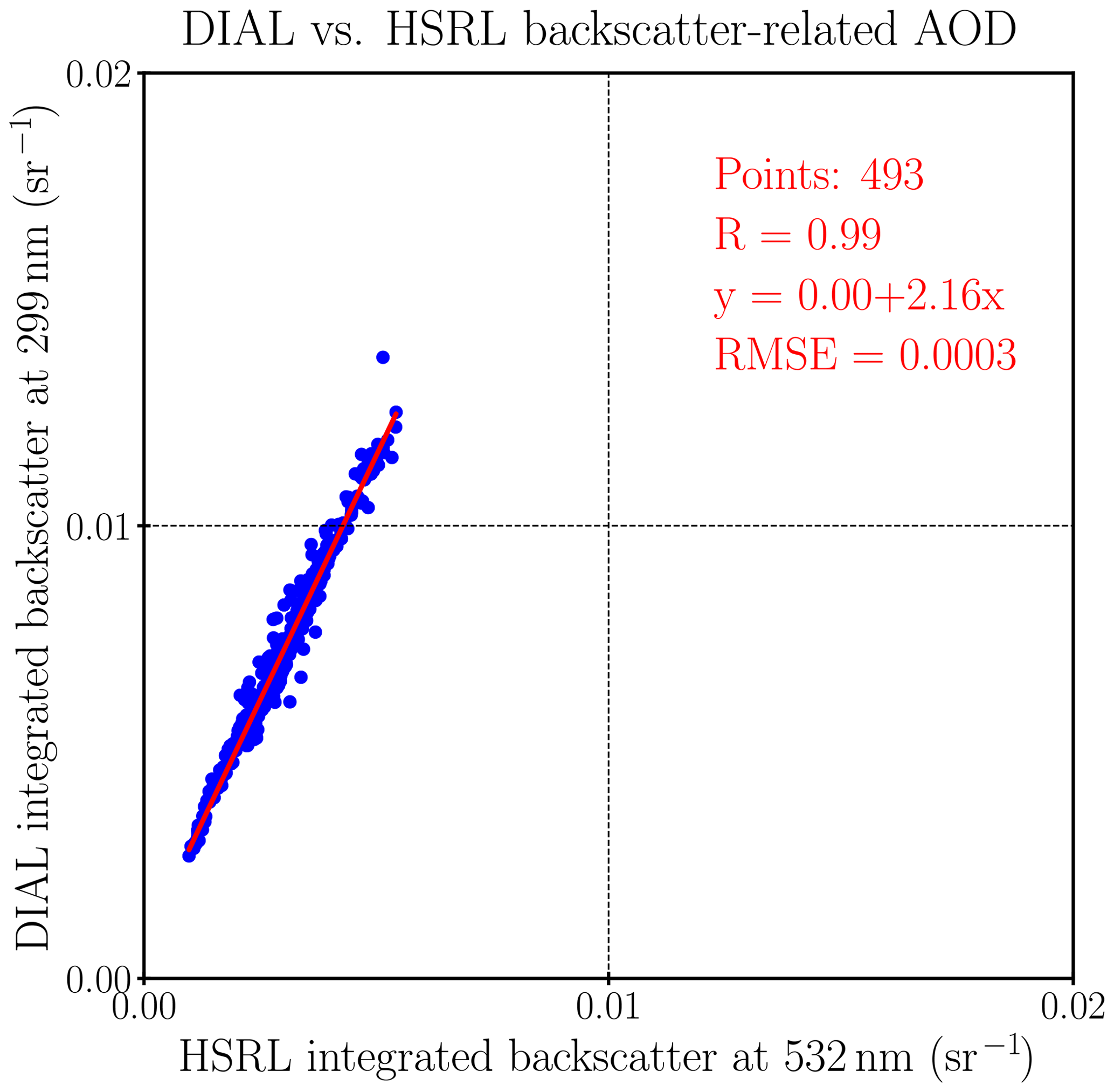
Figure 1 Regression of ozone DIAL- and HSRL-derived integrated aerosol backscatter between 0.4 and 6 km a.s.l. using the best least-squares fit, resulting in a backscatter color ratio of 1.34 for 299–532 nm for four cases in 2013. All the data were taken at Huntsville, AL, USA, during summer 2013.

In practice, aerosol extinction is a more meaningful parameter and more relevant for several applications than backscatter. For the HSRL, the extinction coefficients are linearly converted from the backscatter coefficients by assuming a constant S=55 sr with 20 % uncertainty, as in the same manner as Reid et al. (2017). The estimated Ångström exponent for 299 and 532 nm is 1.49±0.16, using the data in Fig. 1 after considering uncertainties in S for both lidars. The calculated Ångström exponent is different from the backscatter-related wavelength exponent because of the wavelength dependence of S. The Ångström exponent from this study (1.49±0.16) is within a reasonable range compared to previous studies. For example, the Ångström exponent was measured by a Raman lidar to be between 1.35±0.2 and 1.56±0.2 at 355 nm for smoke aerosols in Canada (Strawbridge et al., 2018). The Ångström exponent for urban aerosols was measured to be 1.4±0.5 in Europe and 1.7±0.5 in North America for 355 and 532 nm (Müller et al., 2007).

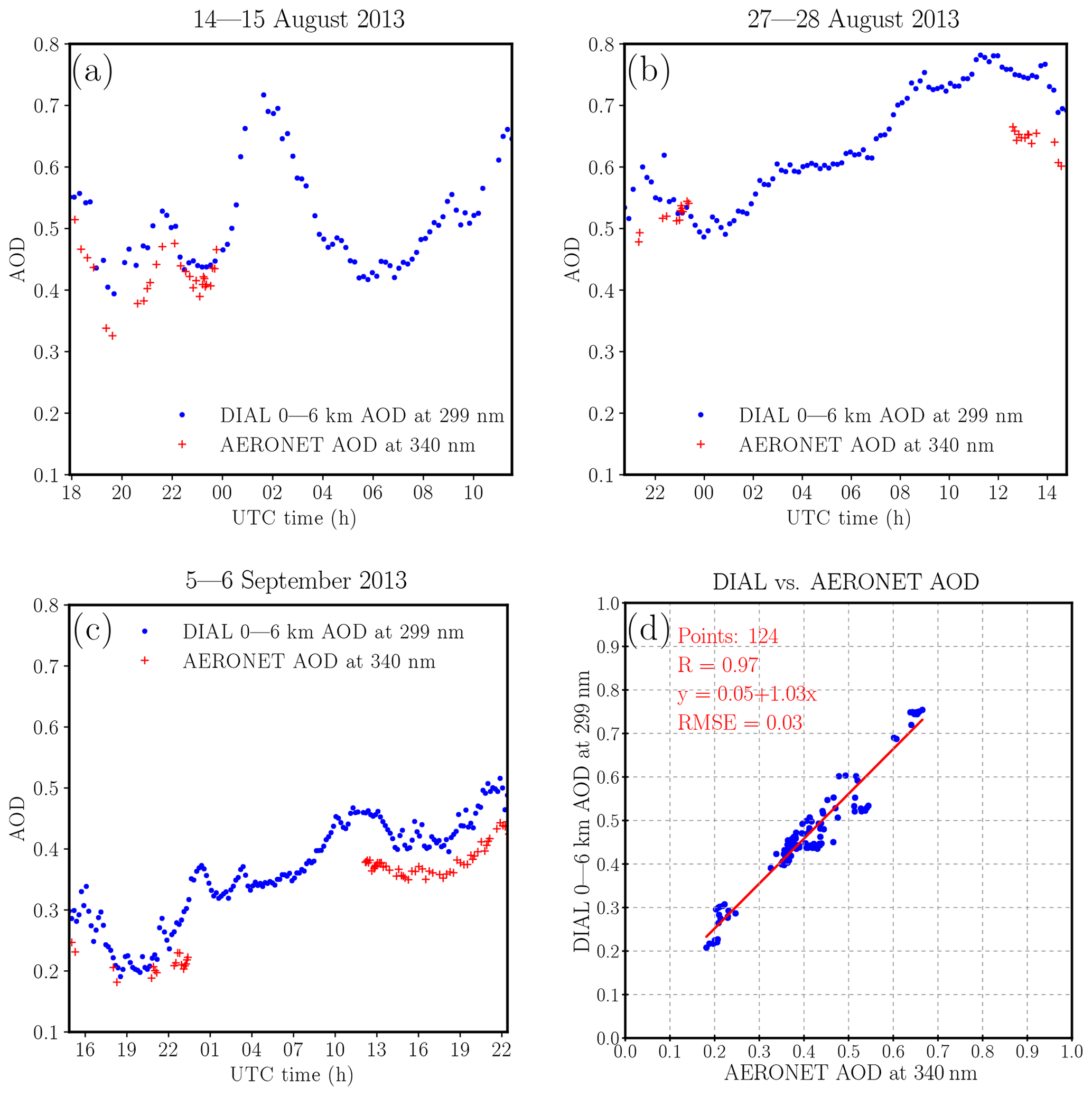
Figure 2 RO₃QET DIAL-derived AOD between 0 and 6 km at 299 nm using S=60 sr compared to colocated AERONET AOD at 340 nm for (a) 14–15 August, (b) 27–28 August, and (c) 5–6 September 2013. (d) Regression of the paired data after the DIAL AOD is interpolated to the times of AERONET AOD measurements.

The AErosol RObotic NETwork (AERONET) (Holben et al., 1998) provides aerosol optical depth (AOD) measurements in eight spectral bands between 340 and 1020 nm with a temporal resolution of about 15 min. The measurement uncertainty for AERONET AOD is within 0.02 and is expected to be larger in the UV bands (Eck et al., 1999; Holben et al., 2001). Even though the measurement is at a different wavelength, the AERONET AOD at 340 nm can provide an additional constraint for the choice of S for the RO₃QET aerosol retrieval, especially since both instruments are at the same location. Figure 2 presents the intercomparison of the RO₃QET lidar-derived AOD at 299 nm and all available AOD data at 340 nm (Smirnov et al., 2000) from the colocated AERONET sun–sky radiometer (data for 21–23 June are unavailable). The near-surface region is assumed to be homogeneous and assigned the same aerosol extinction values as the lowest available 30 m layer from the RO₃QET retrievals. Then, the aerosol extinction coefficients are integrated from 0 to 6 km a.s.l. to calculate the lidar-derived AOD. The omission of aerosol extinction above 6 km and the homogeneity assumption for the near-surface region are sources of bias for the comparison since the AERONET instrument measures the total column AOD. The lidar has more data and higher temporal resolution; therefore, the lidar-derived AOD is interpolated to the AERONET measurement times. Figure 2 shows that the AOD retrieved by the two instruments has a correlation coefficient of 0.97 and a small RMSE for a total duration of about 31 h. The mean percentage difference between the RO₃QET and AERONET AOD is 15 %±9 %. The S a priori value directly affects the AOD calculation. The lidar-derived AOD is on average 15 % larger than the AERONET AOD due to the shorter wavelength of the lidar measurement, suggesting that the choice of S=60 sr is appropriate. For a rough estimation, the 1σ standard deviation (9 %) of the differences can be considered the uncertainty of S if the variability of these differences are mostly due to the variation in S. Considering that AERONET measures the column-average AOD (with longer temporal integration), has its own uncertainty, and covers only 38 % of the total observational period, our assumption for $S=\mathrm{60}\mathit{\%}\mathrm{sr}\pm \mathrm{20}$ % sr is appropriate for RO₃QET lidar profiling measurements with higher temporal and vertical resolution and should be good enough to cover various uncertainty sources. The colocated AERONET data enhance the credibility of our lidar aerosol retrieval and help evaluate the S a priori value, with the caveat that the 124 paired data covering 31 h are not a large sample set. We do not show the HSRL–AERONET comparison here since Reid et al. (2017) have done so using more extensive data in a visible band taken at the UAH site in summer 2013.

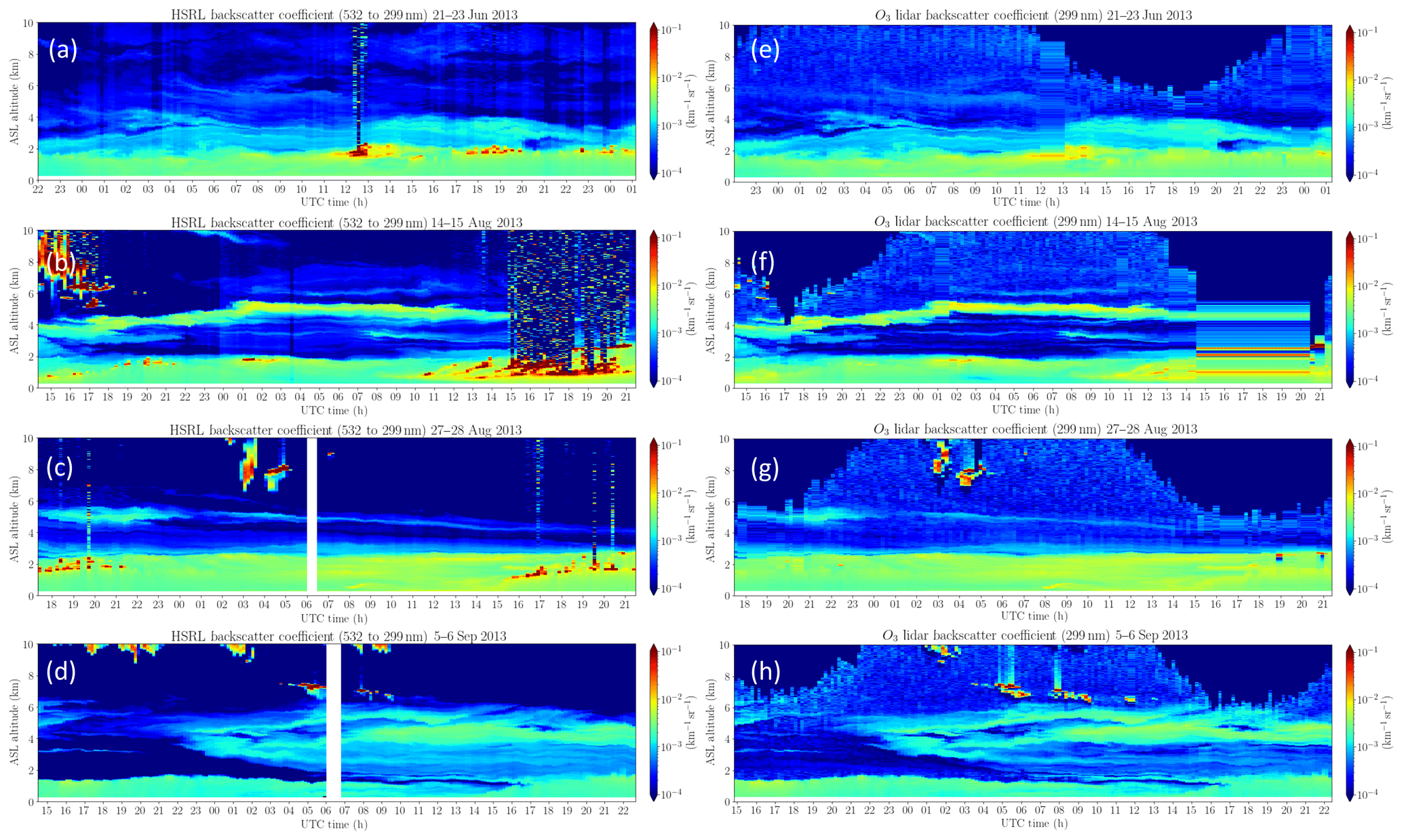
Figure 3 HSRL-converted aerosol backscatter coefficients (a, b, c, d) compared to RO₃QET lidar-derived aerosol backscatter coefficients at 299 nm (e, f, g, h), with 10 min temporal resolution and 30 m vertical resolution. The data were taken from 21 to 23 June (a, e), 14–15 August (b, f), 27–28 August (c, g), and 5–6 September (d, h) 2013. The HSRL-converted aerosol backscatter coefficients are scaled from the original retrievals at 532 to 299 nm using Eq. (1) and å_β=1.34.

Figure 3 presents the intercomparison of the aerosol backscatter retrieved by the HSRL and the RO₃QET lidar for the four cases in 2013. The HSRL-derived aerosol backscatter coefficients are scaled to 299 nm (represented by “HSRL-converted” hereafter) using the best-fit exponent value å_β=1.34. Some clouds lower than 2 km show up in the HSRL curtains but not in the RO₃QET curtains (e.g., 1500–2100 on 15 August and 1500–2100 on 28 August). These low-cloud-contaminated data were discarded in the RO₃QET lidar preprocessing program since the ozone lidar probes the atmosphere with a shorter wavelength than the HSRL and is, therefore, more affected by cloud interference. Profiles with clouds higher than 2 km measured by RO₃QET were retained, and the aerosol retrievals below the clouds were used for the range-resolving intercomparisons.

In terms of the aerosol measurement evaluation, we pay attention to the two capabilities of the RO₃QET lidar: measuring the PBL diurnal evolution and measuring free-tropospheric smoke layers. In Fig. 3, the PBL heights measured by the two lidars, which are identified by large aerosol gradients, are highly consistent for all cases. The development of the convective mixing layer in the early morning, an important process responsible for surface ozone increase, can be visually identified in most RO₃QET curtains (e.g., 14:00–17:00 UTC or 09:00–12:00 LT (local time) in Fig. 3h). The aerosol structures and evolution in the free troposphere measured by the RO₃QET lidar are highly similar to those measured by the HSRL. For example, the RO₃QET lidar captured an extremely thin aerosol layer at ∼5 km altitude on 27–28 August (Fig. 3g), which probably originated from the Pacific Northwest fire and has been discussed by Reid et al. (2017). The large aerosol uncertainties for the RO₃QET lidar at far ranges are consistent with expectation. As demonstrated in Appendix B, aerosol retrieval uncertainties due to lidar-signal measurement error and the boundary value chosen at the reference altitude, which are two of the most important sources of uncertainty, increase with altitude and may exceed 100 % at ∼7 km .

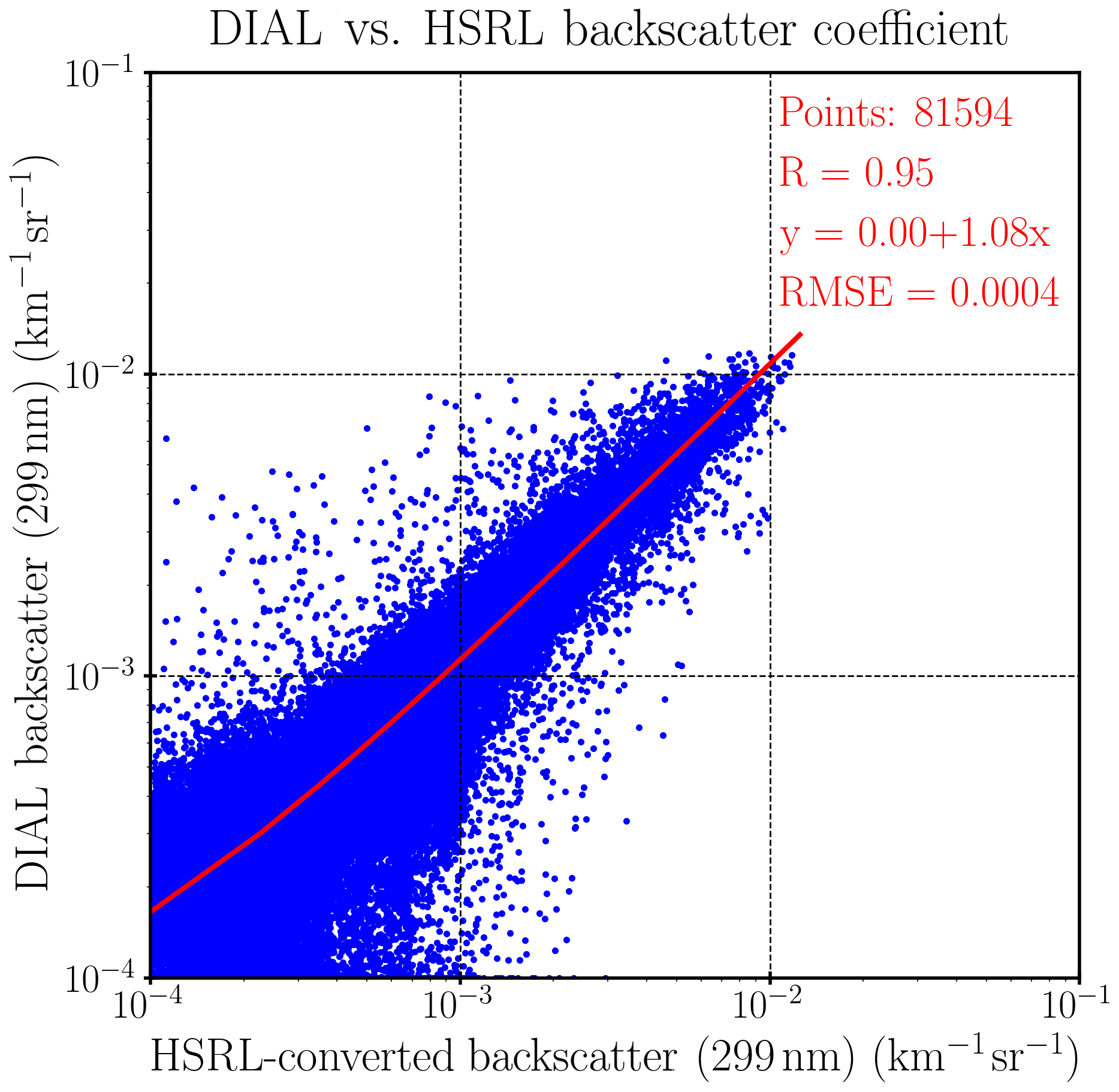
Figure 4 Regression of ozone lidar measured and HSRL-converted aerosol backscatter coefficients (interpolated to 299 nm with å_β=1.34) with 30 m vertical resolution and 10 min temporal resolution. The regression line is a little curved in the logarithmic scale because the intercept is not exactly zero.

To evaluate the range-resolving capability of the ozone lidar for aerosol retrieval, we intercompared the aerosol backscatter coefficients, for all cases, from the two instruments with a 10 min temporal resolution and a 30 m vertical resolution after filtering out cloud-contaminated data, as shown in Fig. 4. The high correlation coefficient of 0.95 suggests that the RO₃QET lidar can capture the aerosol variability with high spatiotemporal resolution. The correlation coefficient (0.95) between the two high vertical resolution retrievals is slightly lower than that between the RO₃QET and column-averaged HSRL retrievals (0.99; see Fig. 1) due to less vertical averaging. The HSRL-converted backscatter is calculated using å_β=1.34 and the regression equation in Fig. 1. We expect the slope of the data in Fig. 4 to be very close to 1. However, the actual slope is 1.08, reflecting the fact that there are a large fraction of points with small aerosol backscatter and larger residuals in clean air (low aerosol) regions. This is not surprising since the HSRL has higher measurement precision than the RO₃QET lidar so that their relative differences in clean air regions can be large.

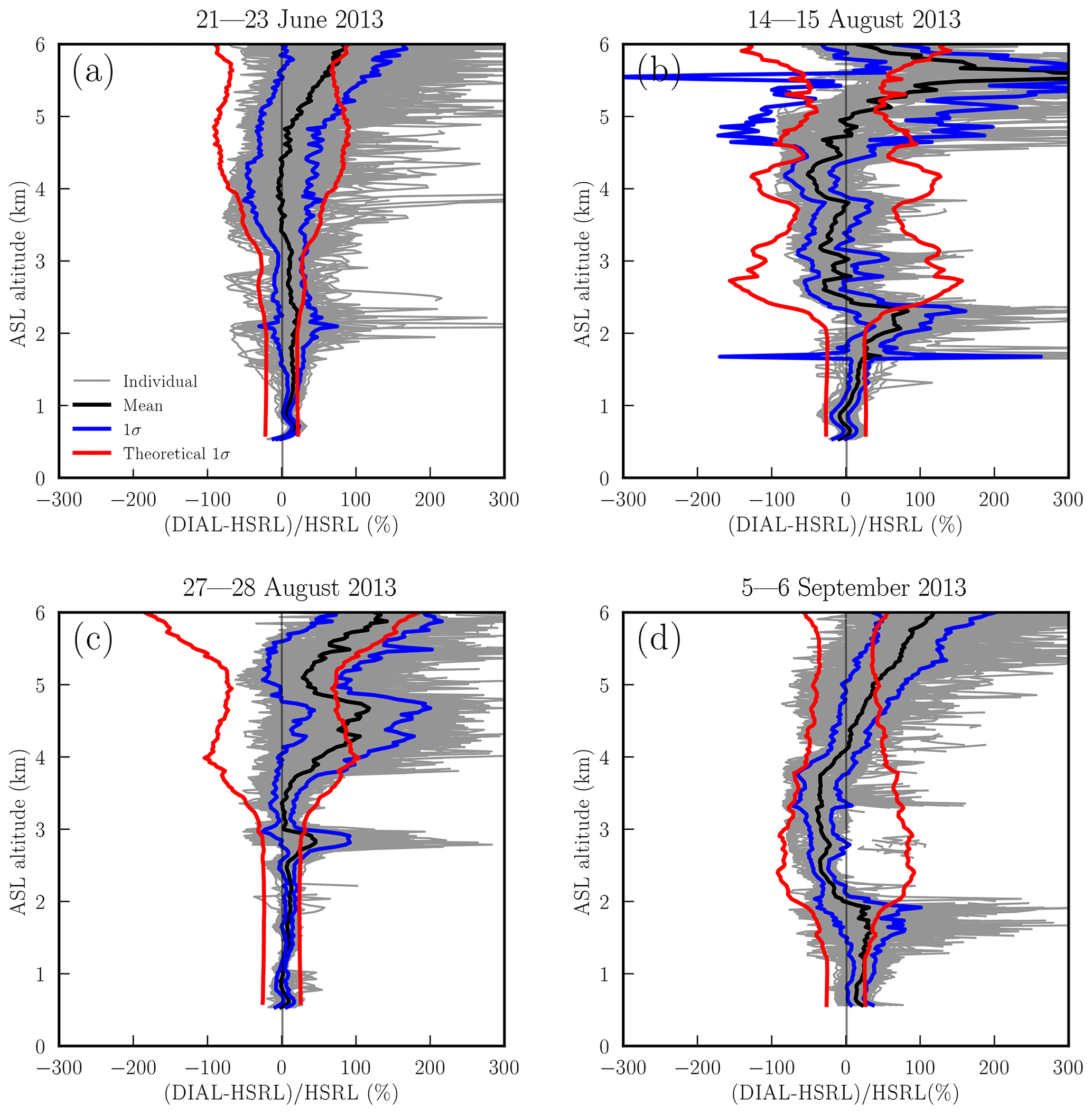
Figure 5 Relative differences between RO₃QET- and HSRL-converted aerosol backscatter measurements, (RO₃QET-HSRL)/HSRL, made from (a) 21–23 June, (b) 14–15 August, (c) 27–28 August, and (d) 5–6 September 2013. The gray and black lines represent the differences for the 10 min individual aerosol backscatter profiles and their mean, respectively. The blue lines represent the actual 1σ of the differences compared to the theoretical 1σ (red lines) of the RO₃QET lidar aerosol measurement.

Figure 5 presents the mean and 1σ standard deviations of the relative differences between RO₃QET and HSRL retrievals, (RO₃QET-HSRL)/HSRL, to be compared with the theoretical 1σ error calculated as outlined in Appendix B. The HSRL measurements are considered the “true” values to be compared with the RO₃QET measurements. Both the theoretical and actual 1σ values generally increase with altitude. The actual differences between RO₃QET and HSRL measurements are mostly within or of comparable order of magnitude to the theoretical calculation of the RO₃QET measurement uncertainties. The structures of the theoretical uncertainties are consistent with the actual differences at most altitudes, with few exceptions. For example, the large discrepancies (red lines compared to blue lines in Fig. 5) occurring at ∼4.5 km in Fig. 5c and ∼1.5 km in Fig. 5d are primarily because of small-number division effects for the extremely clean atmospheric layers (also see Fig. 3). Aerosol backscatter of clean air can be accurately measured by the HSRL, but it may be beyond the measurement sensitivity of RO₃QET.

In Fig. 5, the RO₃QET-measured aerosols are generally higher than the HSRL-measured aerosols between 5 and 6 km, so the RO₃QET-HSRL differences are biased to positive altitude values. These positive biases can be due to two reasons. First, the RO₃QET-derived aerosol extinction above 5 km is obviously larger than that from HSRL during daytime due to the solar background impact, which is especially strong in the summer. The relative differences are even worse in clean (compared to turbid) regions during the daytime because of the small-number division effect mentioned earlier. It can be seen from Fig. 3 that RO₃QET nighttime retrievals above 5 km and daytime retrievals below 5 km are relatively good due to either lower solar background or larger lidar signal resulting in better SNR. There were both clean and smoky layers between 5 and 6 km for the four cases; therefore, the positive differences cannot be explained solely by the lower capability of RO₃QET for measuring clean air. We hypothesize that another reason causing the positive differences between 5 and 6 km is the underestimated backscatter color ratio for the smoke aerosols. We converted the HSRL backscatter from 532 to 299 nm using a constant backscatter color ratio, 1.34, which represents an average for the column-integrated backscatter. The most significant contribution to integrated backscatter comes from PBL aerosols, which are mostly urban aerosols with a lower backscatter color ratio than either fresh or aged smoke (Burton et al., 2012; Cattrall et al., 2005). The uncertainty of the backscatter color ratio was not considered in the error budget of the aerosol retrieval. In addition, we ignored the measurement uncertainty of the HSRL. Therefore, the general agreement of theoretical estimates of aerosol retrieval uncertainties and the actual errors suggests that our analysis of the uncertainty sources in Appendix B is reasonable.

4 Conclusions

We have evaluated the aerosol retrievals at 299 nm from the RO₃QET ozone lidar using both aerosol retrievals at 532 nm from the University of Wisconsin HSRL and AERONET AOD data at 340 nm from coincident observations at Huntsville, AL, in 2013. The integrated backscatter coefficients below 6 km a.s.l. from RO₃QET and HSRL are highly correlated, with a Pearson coefficient of 0.99 after excluding cloud-contaminated data. The aerosol profiles of backscatter coefficients at 30 m vertical and 10 min temporal resolution retrieved by RO₃QET are also highly correlated with those from the HSRL with a coefficient of 0.95 suggesting that the ozone lidar is capable of providing reliable aerosol structure information at high spatiotemporal resolution. Intercomparison of the backscatter product was performed to avoid additional uncertainty caused by the lidar ratio (S) assumption needed for the HSRL aerosol extinction retrieval. The RO₃QET-measured AOD below 6 km a.s.l. is also highly correlated with the AERONET-measured AOD, with a correlation coefficient of 0.97. The 340 nm band of the AERONET AOD data is closest to the ozone lidar wavelength among the available instruments and can, therefore, provide a constraint for the S assumption for the ozone lidar. Analysis of the intercomparison of AERONET and RO₃QET data confirms that our choice of S=60 sr at 299 nm is appropriate. The aerosol retrieval algorithm and its error budget are shown in Appendix B. The primary uncertainty sources for the aerosol lidar retrieval are errors in lidar-signal measurement, boundary value assumption, air density calculation, S a priori value, and ozone profile input. The uncertainty in S assumption is a dominant source at near range, while the lidar-signal measurement and boundary value errors dominate at far range, as shown in Fig. B1 for a sample scenario. Within the middle range (PBL top to about 7 km), the air density calculation error is essential and is larger or comparable to the lidar-signal measurement error. The total uncertainty generally increases with altitude from about 15 % in the PBL to consistently higher than 100 % above 7 km. Theoretical estimates of the error budget are generally consistent with the RO₃QET and HSRL measurement differences.

By assuming a constant S of 60 sr at 299 nm, the backscatter coefficients measured by RO₃QET and HSRL are related by a backscatter color ratio (backscatter-related exponent) of 1.34±0.11 for 299 and 532 nm. The extinction-related Ångström exponent, which is more relevant for various applications, is estimated to be 1.49±0.16 by assuming S=55 sr for the HSRL at 532 nm. These exponents represent a summertime average for a mixture of urban pollution and fire smoke. Separation of aerosol types was not done in this work, although we recognize that S and Ångström exponent vary with the aerosol phase function and size distribution. Aerosol correction for ozone lidar retrievals will be described in a subsequent paper.

Appendix A: Aerosol retrieval algorithm

The ozone DIAL solution can be written as follows:

$$\begin{array}{}\text{(A1)}& n_{\left(r\right)}={\displaystyle \frac{-\mathrm{1}}{\mathrm{2}\mathrm{\Delta }\mathit{\sigma }}}\times {\displaystyle \frac{\mathrm{d}}{\mathrm{d}r}}\left[\ln {\displaystyle \frac{P_{\mathrm{on}\left(r\right)}}{P_{\mathrm{off}\left(r\right)}}}\right]+\left[B\right]+\left[E\right],\end{array}$$

where n_(r) is the ozone number density at range r; Δσ is the differential ozone absorption cross section; P_on(r) and P_off(r) are the backscattered online and offline lidar returns; and [B] and [E] represent the differential backscatter and extinction terms (Browell et al., 1985), respectively, including both molecular and aerosol components. The first term of the right-hand side of Eq. (A1) is often called the signal term. The subscripts “on” and “off” represent 289 and 299 nm, respectively, in this study. The aerosol extinction coefficients at 299 nm are calculated using the following procedure.

A first-order Savitzky–Golay differentiation filter with a second-degree polynomial and variable fitting window widths is applied on $\ln \frac{P_{\mathrm{on}\left(r\right)}}{P_{\mathrm{off}\left(r\right)}}$ to compute the signal term. This smoothing method can accommodate the rapid decay of the lidar signal with altitude to provide sufficient SNR for ozone retrievals by appropriate selection of smoothing window widths (Leblanc et al., 2016).

By canceling the lidar constant using the two lidar equations at ranges r and r+Δr for 299 nm, the aerosol backscatter coefficients at range r can be expressed as (Uchino et al., 1980)

$$\begin{array}{}\text{(A2)}& \begin{array}{rl}{\mathit{\beta }}_{\mathrm{A}}\left(r\right)& =-{\mathit{\beta }}_{\mathrm{M}}\left(r\right)+{\displaystyle \frac{Z\left(r\right)}{Z(r+\mathrm{\Delta }r)}}\left[{\mathit{\beta }}_{\mathrm{A}}\left(r+\mathrm{\Delta }r\right)\right.\\ & \left.+{\mathit{\beta }}_{\mathrm{M}}\left(r+\mathrm{\Delta }r\right)\right]\exp \left\{-\mathrm{2}\mathrm{\Delta }r\left[{\mathit{\alpha }}_{\mathrm{A}}\left(r+{\displaystyle \frac{\mathrm{\Delta }r}{\mathrm{2}}}\right)\right.\right.\\ & \left.\left.+{\mathit{\alpha }}_{\mathrm{M}}\left(r+{\displaystyle \frac{\mathrm{\Delta }r}{\mathrm{2}}}\right)+{\mathit{\alpha }}_{\mathrm{O}\mathrm{3}}\left(r+{\displaystyle \frac{\mathrm{\Delta }r}{\mathrm{2}}}\right)\right]\right\},\end{array}\end{array}$$

where β_A(r) and β_M(r) are aerosol and molecular backscatter coefficients at range r, respectively; Z(r)=P_offr² is the range-corrected lidar signal at 299 nm; and α_A(r+Δr/2), α_M(r+Δr/2), and ${\mathit{\alpha }}_{{\mathrm{O}}_{\mathrm{3}}}(r+\mathrm{\Delta }r$/2) represent the average aerosol, molecular, and ozone extinction coefficients, respectively, between ranges r and r+Δr. Assuming that the 299 nm lidar ratio, S=α_A/β_A, is constant with the range at 60 sr for this study and further assuming that

$$\begin{array}{}\text{(A3)}& {\mathit{\alpha }}_{\mathrm{A}}(r+{\displaystyle \frac{\mathrm{\Delta }r}{\mathrm{2}}})\approx {\mathit{\alpha }}_{\mathrm{A}}\left(r+\mathrm{\Delta }r\right)=S{\mathit{\beta }}_{\mathrm{A}}\left(r+\mathrm{\Delta }r\right),\end{array}$$

Eq. (A2) contains only two unknown variables: the aerosol backscatter coefficient β_A(r+Δr) and ozone extinction coefficient ${\mathit{\alpha }}_{{\mathrm{O}}_{\mathrm{3}}}(r+\mathrm{\Delta }r/\mathrm{2}$), which requires knowledge of the ozone number density $n_{(r+\mathrm{\Delta }r/\mathrm{2})}$. Molecular backscatter and extinction can be computed from nearby radiosonde data or a model with acceptable accuracy. For the first iteration step, $n_{(r+\mathrm{\Delta }r/\mathrm{2})}$ can be computed from the signal term in Eq. (A1). By assuming a start value β_A(ref) at a reference range and a constant S with range, β_A(r) can be solved by Eq. (A2). Then, the first β_A(r) profile is substituted back into Eq. (A2) to compute the second estimate by using a more accurate form for ${\mathit{\alpha }}_{\mathrm{A}}(r+\mathrm{\Delta }r/\mathrm{2}$) as

$$\begin{array}{}\text{(A4)}& {\mathit{\alpha }}_{\mathrm{A}}\left(r+{\displaystyle \frac{\mathrm{\Delta }r}{\mathrm{2}}}\right)=S\left[{\mathit{\beta }}_{\mathrm{A}}\left(r+\mathrm{\Delta }r\right)+{\mathit{\beta }}_{\mathrm{A}}^{\prime }\left(r\right)\right]/\mathrm{2},\end{array}$$

where ${\mathit{\beta }}_{\mathrm{A}}^{\prime }\left(r\right)$ represents the value from the first estimate. Typically, a stable solution for β_A(r), which does not change significantly from one iteration step to the next, can be obtained with only three iterations of Eqs. (A2) and (A4).

The correction terms, [B] and [E], in Eq. (A1) are calculated by the Browell et al. (1985) approximation, assuming a power-law dependence with wavelength for the aerosol extinction and choosing an appropriate Ångström exponent. Since this paper focuses only on aerosol retrievals, the details of the ozone corrections will be described in a future article.

Aerosol profiles computed for the three altitude channels are finally merged into a single profile in their overlapping altitude zones: 0.5–1 km for channels 1 and 2 and 1.5–2 km for channels 2 and 3.

Appendix B: Error budget of the aerosol retrieval

Now we investigate five primary error sources affecting each term on the right-hand side of Eq. (A2). In the following section, we use the notation Δ to represent the absolute uncertainty and δ to represent the relative uncertainty. For a function Y, derived from several measurement variables x₁, x₂, …, the uncertainty in Y can be estimated by the following expression using the first-order Taylor expansion approximation when these variables are independent (Taylor, 1997):

$$\begin{array}{}\text{(B1)}& \mathrm{\Delta }{Y}^{\mathrm{2}}={\left(\mathrm{\Delta }{x}_{\mathrm{1}}{\displaystyle \frac{\partial Y}{\partial x_{\mathrm{1}}}}\right)}^{\mathrm{2}}+{\left(\mathrm{\Delta }{x}_{\mathrm{2}}{\displaystyle \frac{\partial Y}{\partial x_{\mathrm{2}}}}\right)}^{\mathrm{2}}+\mathrm{\dots }\end{array}$$

B1 Lidar-signal measurement error

The error source to determine the normalized lidar-signal ratio term $\frac{Z\left(r\right)}{Z(r+\mathrm{\Delta }r)}$ is the lidar-signal measurement error ΔP. Although ΔP may be due to various processes such as inaccurate dead-time correction, inaccurate background subtraction, and signal-induced noise, its dominant component is the lidar-signal statistical uncertainty (often called lidar-signal detection noise) and is typically assumed to obey a Poisson distribution. Assuming no error in deciding r, by using Eqs. (A2) and (B1) we obtain the uncertainty of the aerosol backscatter owing to lidar-signal measurement error, $\mathrm{\Delta }{\mathit{\beta }}_{\mathrm{A}}^{\mathrm{sig}}\left(r\right)$, relative to the total backscatter as

$$\begin{array}{}\text{(B2)}& {\displaystyle \frac{\mathrm{\Delta }{\mathit{\beta }}_{\mathrm{A}}^{\mathrm{sig}}\left(r\right)}{{\mathit{\beta }}_{\mathrm{A}}\left(r\right)+{\mathit{\beta }}_{\mathrm{M}}\left(r\right)}}=\sqrt{{\left[\mathit{\delta }P\left(r\right)\right]}^{\mathrm{2}}+{\left[\mathit{\delta }P\left(r+\mathrm{\Delta }r\right)\right]}^{\mathrm{2}}},\end{array}$$

where P(r) represents lidar-signal counts at r after omitting the wavelength subscript (i.e., 299 nm), and δP(r) is just the inverse of SNR. Equation (B2) means that the uncertainty of the aerosol backscatter coefficient due to lidar-signal measurement is determined by the lidar SNR similarly to other remote-sensing detection techniques. Consequently, its relative uncertainty can be written as

$$\begin{array}{}\text{(B3)}& \mathit{\delta }{\mathit{\beta }}_{\mathrm{A}}^{\mathrm{sig}}\left(r\right)=\left({\displaystyle \frac{\mathrm{1}}{B\left(r\right)}}+\mathrm{1}\right)\sqrt{{\left[\mathit{\delta }P\left(r\right)\right]}^{\mathrm{2}}+{\left[\mathit{\delta }P\left(r+\mathrm{\Delta }r\right)\right]}^{\mathrm{2}}},\end{array}$$

where $B\left(r\right)={\mathit{\beta }}_{\mathrm{A}}\left(r\right)/{\mathit{\beta }}_{\mathrm{M}}\left(r\right)$ is the aerosol-to-molecular backscatter ratio. As expected, $\mathit{\delta }{\mathit{\beta }}_{\mathrm{A}}^{\mathrm{sig}}\left(r\right)$ has a reverse relationship with β_A(r) since it is a relative uncertainty. Figure B1 shows an example of the uncertainty budget for a 10 min lidar data profile. The aerosol retrieval uncertainty due to the lidar-signal measurement error generally increases with altitude primarily because of the rapidly decaying lidar SNR.

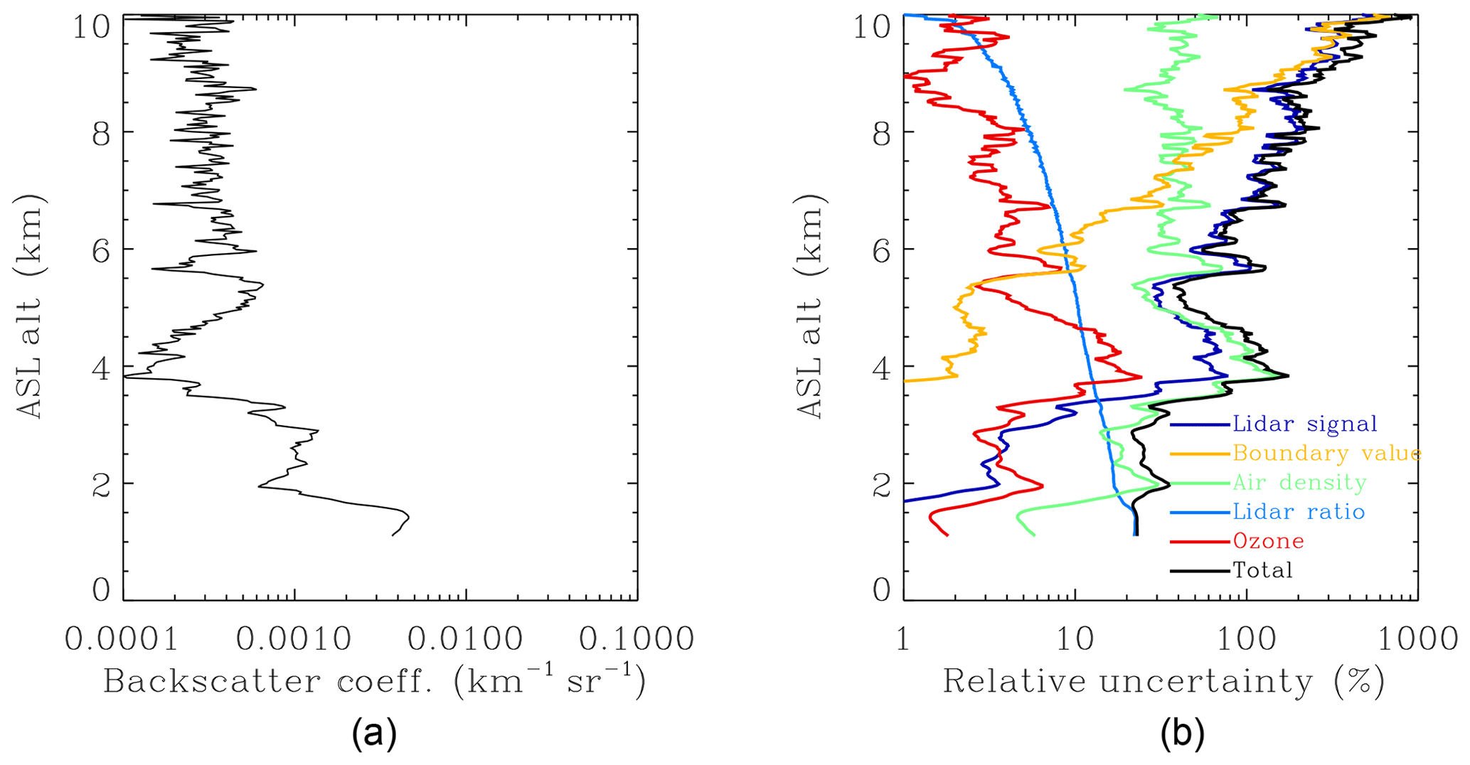
Figure B1 An example of (a) aerosol backscatter profile retrieved from 10 min ozone lidar data at about 08:30 UTC on 22 June 2013 and (b) the retrieval error budget for different uncertainty sources. The lidar data were from the channel-3 receiving system, which covered most of the measurement altitude range, and was arbitrarily chosen for a cloud-free scenario.

B2 Boundary value error

According to Eq. (A2), the uncertainty of the aerosol backscatter at r, β_A(r) , can be induced by the uncertainty of the backscatter at r+Δr, β_A(r+Δr), due to the iterative computation method. The error propagation between the adjacent altitudes can be determined by their partial differential relationship. Using the traditional far-end solution by assuming that the air is clean at a reference altitude, the aerosol uncertainty due to the inaccurate boundary value assumption propagates downward based on the following equation:

$$\begin{array}{}\text{(B4)}& \begin{array}{rl}\mathit{\delta }{\mathit{\beta }}_{\mathrm{A}}^{\mathrm{BV}}\left(r\right)& =\mathit{\delta }{\mathit{\beta }}_{\mathrm{A}}\left(r+\mathrm{\Delta }r\right)\left[{\displaystyle \frac{\mathrm{1}+\frac{\mathrm{1}}{B\left(r\right)}}{\mathrm{1}+\frac{\mathrm{1}}{B\left(r+\mathrm{\Delta }r\right)}}}\right]\\ & \left\{\mathrm{1}-\mathrm{2}S\mathrm{\Delta }r{\mathit{\beta }}_{\mathrm{A}}\left(r+\mathrm{\Delta }r\right)\left[\mathrm{1}+{\displaystyle \frac{\mathrm{1}}{B\left(r+\mathrm{\Delta }r\right)}}\right]\right\}.\end{array}\end{array}$$

The yellow line in Fig. B1 represents the relative uncertainty of backscatter retrieval due to the boundary value assumption, $\mathit{\delta }{\mathit{\beta }}_{\mathrm{A}}^{\mathrm{BV}}\left(r\right)$, when δβ_A(r_b)=1000 % (i.e., 10 times overestimate at r_b=10 km). Despite a large overestimate at the reference altitude, $\mathit{\delta }{\mathit{\beta }}_{\mathrm{A}}^{\mathrm{BV}}\left(r\right)$ decreases toward the ground to less than 10 % below 5.5 km and less than 1 % below 3.5 km. Simulations demonstrate that $\mathit{\delta }{\mathit{\beta }}_{\mathrm{A}}^{\mathrm{BV}}\left(r\right)$ for an underestimation of δβ_A(r_b) (not shown) is better than that for an overestimation, indicating that the boundary value is preferred at a smaller value. As suggested by Eq. (B4), $\mathit{\delta }{\mathit{\beta }}_{\mathrm{A}}^{\mathrm{BV}}\left(r\right)$ is affected by both S and B. Larger S (if it is correct) results in smaller $\mathit{\delta }{\mathit{\beta }}_{\mathrm{A}}^{\mathrm{BV}}\left(r\right)$ and, therefore, aerosol retrieval errors converge to zero faster. In other words, the smaller the value of S is, the more sensitive the aerosol retrieval is to the boundary value error. $\mathit{\delta }{\mathit{\beta }}_{\mathrm{A}}^{\mathrm{BV}}\left(r\right)$ decreases with an increase of B(r). This means that $\mathit{\delta }{\mathit{\beta }}_{\mathrm{A}}^{\mathrm{BV}}\left(r\right)$ is less affected by the assumed value of β_A(r_b) when the aerosol backscatter becomes more important relative to molecular backscatter, which occurs at longer wavelengths or under turbid air conditions. It is to be noted that δβ_A(r_b) is between −1 and +∞ so that the distribution of $\mathit{\delta }{\mathit{\beta }}_{\mathrm{A}}^{\mathrm{BV}}\left(r\right)$ is asymmetric with the zero axis.

In terms of the influence of the boundary value error, we have compared our calculation with an analytical solution proposed by Kovalev and Moosmüller (1994) (not shown); the results are almost identical. Aerosol retrieval uncertainty due to incorrect boundary value assumption tends to converge to zero towards the lidar. It is negligible at lower altitudes, especially in the PBL, when the air is turbid.

B3 Air density error

According to Eq. (A2), the air density profile affects ${\mathit{\beta }}_{\mathrm{M}}\left(r\right),{\mathit{\beta }}_{\mathrm{M}}(r+\mathrm{\Delta }r)$, and the optical depth (or transmittance). Similarly, we can derive the relative uncertainty in aerosol backscatter owing to the uncertainty in the air density profile as

$$\begin{array}{}\text{(B5)}& \begin{array}{rl}\mathit{\delta }& {\mathit{\beta }}_{\mathrm{A}}^{\mathrm{AD}}\left(r\right)=\\ & \sqrt{\mathit{\left\{}{\displaystyle \frac{\mathit{\delta }{\mathit{\beta }}_{\mathrm{M}}\left(r\right)}{B\left(r\right)}}\right[\mathrm{1}+S_{\mathrm{m}}\mathrm{\Delta }r{\mathit{\beta }}_{\mathrm{A}}\left(r\right)+S_{\mathrm{m}}\mathrm{\Delta }r{\mathit{\beta }}_{\mathrm{M}}\left(r\right)]{\mathit{\}}}^{\mathrm{2}}}\\ & \stackrel{\mathrm{‾}}{+\mathit{\left\{}{\displaystyle \frac{\mathit{\delta }{\mathit{\beta }}_{\mathrm{M}}\left(r+\mathrm{\Delta }r\right)\left[\frac{\mathrm{1}}{B\left(r\right)}+\mathrm{1}\right]}{B\left(r+\mathrm{\Delta }r\right)+\mathrm{1}}}\right[\mathrm{1}-S_{\mathrm{m}}\mathrm{\Delta }r{\mathit{\beta }}_{\mathrm{A}}\left(r+\mathrm{\Delta }r\right)}\\ & \stackrel{\mathrm{‾}}{-S_{\mathrm{m}}\mathrm{\Delta }r{\mathit{\beta }}_{\mathrm{M}}\left(r+\mathrm{\Delta }r\right)]{\mathit{\}}}^{\mathrm{2}}}.\end{array}\end{array}$$

S_m represents the molecular extinction-to-backscatter ratio, which is a constant (8π∕3). The two parts in the square root are the components due to the uncertainties at r and r+Δr. Each component includes the influences from both molecular backscatter and optical depth. When Δr is small, the contribution of the optical depth error is much smaller than that of the molecular backscatter error, so Eq. (B4) can be approximated as

$$\begin{array}{}\text{(B6)}& \mathit{\delta }{\mathit{\beta }}_{\mathrm{A}}^{\mathrm{AD}}\left(r\right)\approx \sqrt{\mathrm{2}}{\displaystyle \frac{\mathit{\delta }{\mathit{\beta }}_{\mathrm{M}}\left(r\right)}{B\left(r\right)}}.\end{array}$$

It is to be noted that Δβ_M(r) and Δβ_M(r+Δr) are independent errors as assumed in Eq. (B1). If they are correlated, Eq. (B5) will partly cancel out with their covariance term, which is not shown in Eq. (B1). Due to the nature of the iterative computation method, $\mathit{\delta }{\mathit{\beta }}_{\mathrm{A}}^{\mathrm{AD}}(r+\mathrm{\Delta }r)$ affects $\mathit{\delta }{\mathit{\beta }}_{\mathrm{A}}^{\mathrm{AD}}\left(r\right)$ as noted in Eq. (B4), so the aerosol retrieval uncertainty due to air density error will propagate downward. However, model simulation suggests that the systematic error of the air density calculation has little impact on the aerosol retrieval because of the cancelation of the effect at r and r+Δr. Equation (B6) means the uncertainty in the calculation of molecular backscatter will mostly linearly propagate to aerosol backscatter. If the 2σ precisions of a radiosonde are 0.3 K and 0.5 hPa for temperature and pressure measurements (Hurst et al., 2011), the propagated uncertainty onto molecular backscatter is only about 0.1 %. However, the real disturbance of an atmosphere deviating from the actual air density profile may be more significant since there are usually only a few radiosonde profiles available every day. Hence, we assume δβ_M(r) to be 1 %, and the resulting aerosol retrieval uncertainty is represented by the green line in Fig. B1. $\mathit{\delta }{\mathit{\beta }}_{\mathrm{A}}^{\mathrm{AD}}\left(r\right)$ can be tens of percent in the free troposphere and is an important error source for aerosol retrievals (Russell et al., 1979). $\mathit{\delta }{\mathit{\beta }}_{\mathrm{A}}^{\mathrm{AD}}\left(r\right)$ is less than 10 % in the PBL because of more turbid air in that region. Since δβ_M(r) is assumed to be a constant in this example, the variation of $\mathit{\delta }{\mathit{\beta }}_{\mathrm{A}}^{\mathrm{AD}}\left(r\right)$ is mostly a result of varying B(r), which is the aerosol-to-molecular backscatter ratio. Since B(r) generally increases with an increase in wavelength, $\mathit{\delta }{\mathit{\beta }}_{\mathrm{A}}^{\mathrm{AD}}\left(r\right)$ is expected to be smaller at longer wavelengths. Therefore, the aerosol retrieval is less sensitive to the air density error at longer wavelengths.

B4 Lidar ratio error

By using Eqs. (A2) and (B1), the relative uncertainty in aerosol backscatter due to incorrect lidar ratio (S) assumption can be calculated as follows:

$$\begin{array}{}\text{(B7)}& \mathit{\delta }{\mathit{\beta }}_{\mathrm{A}}^S\left(r\right)=\mathrm{2}\left[{\displaystyle \frac{\mathrm{1}}{B\left(r\right)}}+\mathrm{1}\right]\mathrm{\Delta }S{\mathit{\beta }}_{\mathrm{A}}\left(r\right)\mathrm{\Delta }r.\end{array}$$

$\mathit{\delta }{\mathit{\beta }}_{\mathrm{A}}^S\left(r\right)$ due to ΔS at only range r appears to be small, about 1 %, when Δr is specified at 22.5 m. However, ΔS varying with altitude is mostly systematic; therefore, $\mathit{\delta }{\mathit{\beta }}_{\mathrm{A}}^S\left(r\right)$ at every altitude will propagate downward, and these effects will accumulate. The error accumulation is not straightforward to compute as an analytical solution. However, these effects can be simulated numerically. S is highly variable, and it is difficult to estimate its actual uncertainty range. In this study, we assume that δS=20 % (or ΔS=12 sr) according to both a previous study (Müller et al., 2007) and the analysis using the colocated AERONET AOD data at 340 nm. The light blue line in Fig. B1 shows that the accumulative uncertainties in the aerosol backscatter due to ΔS using Eqs. (B7) and (B4) are close to the assumed 20 % uncertainty for δS; $\mathit{\delta }{\mathit{\beta }}_{\mathrm{A}}^S\left(r\right)$ is the largest error source in the PBL, which is the near range of the lidar measurement. $\mathit{\delta }{\mathit{\beta }}_{\mathrm{A}}^S\left(r\right)$ decreases with an increase in wavelength because of increasing B(r). In other words, $\mathit{\delta }{\mathit{\beta }}_{\mathrm{A}}^S\left(r\right)$ is less sensitive to ΔS at longer wavelengths.

B5 Ozone error

Similar to S, the ozone uncertainty affects only the transmittance term in Eq. (A2), and its error propagation on aerosol backscatter retrieval can be expressed as

$$\begin{array}{}\text{(B8)}& \mathit{\delta }{\mathit{\beta }}_{\mathrm{A}}^{{\mathrm{O}}_{\mathrm{3}}}\left(r\right)=\mathrm{2}\left[{\displaystyle \frac{\mathrm{1}}{B\left(r\right)}}+\mathrm{1}\right]\mathrm{\Delta }{\mathit{\alpha }}_{{\mathrm{O}}_{\mathrm{3}}}\left(r\right)\mathrm{\Delta }r.\end{array}$$

$\mathit{\delta }{\mathit{\beta }}_{\mathrm{A}}^{{\mathrm{O}}_{\mathrm{3}}}\left(r\right)$ is proportional to the $\left[\frac{\mathrm{1}}{B\left(r\right)}+\mathrm{1}\right]$ factor and ozone absorption uncertainty, meaning that $\mathit{\delta }{\mathit{\beta }}_{\mathrm{A}}^{\mathrm{O}\mathrm{3}}\left(r\right)$ is smaller at longer wavelengths due to larger aerosol scattering ratio and smaller ozone absorption. When Δr is specified at 22.5 m, $\mathit{\delta }{\mathit{\beta }}_{\mathrm{A}}^{\mathrm{O}\mathrm{3}}\left(r\right)$ is less than 0.3 %. We still simulate the vertical accumulation of $\mathit{\delta }{\mathit{\beta }}_{\mathrm{A}}^{\mathrm{O}\mathrm{3}}\left(r\right)$ using Eq. (B4). As noted earlier, the systematic errors of the DIAL ozone measurement tend to accumulate, while the random errors tend to cancel out. The dominant error source for lidar measurements at the far range is typically the lidar-signal detection noise, a type of random error. Therefore, for purposes of estimation, we assume a 5 % constant DIAL retrieval uncertainty primarily covering the uncertainties due to ozone absorption cross section, non-ozone gas interference, and signal saturation effect (Leblanc et al., 2018; Wang et al., 2017). As shown in Fig. B1, the simulated aerosol retrieval uncertainty due to ozone is relatively minor and is less than 5 % at most altitudes.

In summary, the uncertainties in aerosol backscatter retrieval for the ozone lidar are controlled by ΔS at near ranges (i.e., in the PBL) where the air is most turbid and are determined by both the lidar-signal detection error and inaccurate boundary value assumption at far ranges (higher than 7 km) where the air is typically clear. In the middle range of the lidar measurement (PBL top to 7 km), the air density calculation error may become a significant error source for aerosol retrieval and may have a comparable influence on the aerosol retrieval as the lidar-signal measurement error. Relative to the four above uncertainty sources, ozone DIAL retrieval error is relatively unimportant, especially in the lower altitudes where lidar SNR is large enough. All the uncertainty terms are affected by the aerosol-to-molecular backscatter ratio, B(r), which represents the relative importance of the aerosol component in both extinction and backscatter processes. Based on the above uncertainty budget analysis, we conclude that the RO₃QET lidar is capable of measuring aerosol profile reliably below 6 km with the current laser output power.