the Creative Commons Attribution 4.0 License.
the Creative Commons Attribution 4.0 License.
 | 13 Oct 2020
Measurements of PM2.5 with PurpleAir under atmospheric conditions
Karin Ardon-Dryer
Yuval Dryer
Jake N. Williams
Nastaran Moghimi
The PurpleAir PA-II unit is a low-cost sensor for monitoring changes in the concentrations of particulate matter (PM) of various sizes. There are currently more than 10 000 PA-II units in use worldwide; some of the units are located in areas where no other reference air monitoring system is present. Previous studies have examined the performance of these PA-II units (or the sensors within them) in comparison to a co-located reference air monitoring system. However, because PA-II units are installed by PurpleAir customers, most of the PA-II units are not co-located with a reference air monitoring system and, in many cases, are not near one. This study aims to examine how each PA-II unit performs under atmospheric conditions when exposed to a variety of pollutants and PM2.5 concentrations (PM with an aerodynamic diameter smaller than 2.5 µm), when at a distance from the reference sensor. We examine how PA-II units perform in comparison to other PA-II units and Environmental Protection Agency (EPA) Air Quality Monitoring Stations (AQMSs) that are not co-located with them. For this study, we selected four different regions, each containing multiple PA-II units (minimum of seven per region). In addition, each region needed to have at least one AQMS unit that was co-located with at least one PA-II unit, all units needed to be at a distance of up to 5 km from an AQMS unit and up to 10 km between each other. Correction of PM2.5 values of the co-located PA-II units was implemented by multivariate linear regression (MLR), taking into account changes of temperature and relative humidity. The fit coefficients, received from the MLR, were then used to correct the PM2.5 values in all the remaining PA-II units in the region. Hourly PM2.5 measurements from each PA-II unit were compared to those from the AQMSs and other PA-II units in its region. The correction of the PM2.5 values improved the R-squared value (R2), root-mean-square error (RMSE), and mean absolute error (MAE) and slope values between all units. In most cases, the AQMSs and the PA-II units were found to be in good agreement (75 % of the comparisons had a R2>0.8); they measured similar values and followed similar trends; that is, when the PM2.5 values measured by the AQMSs increased or decreased, so did those of the PA-II units. In some high-pollution events, the corrected PA-II had slightly higher PM2.5 values compared to those measured by the AQMS. Distance between the units did not impact the comparison between units. Overall, the PA-II unit, after corrections of PM2.5 values, seems to be a promising tool for identifying relative changes in PM2.5 concentration with the potential to complement sparsely distributed monitoring stations and to aid in assessing and minimizing the public exposure to PM.
- Article
(6022 KB) - Full-text XML
-
Supplement
(13028 KB) - BibTeX
- EndNote


Atmospheric particulate matter (PM) with an aerodynamic diameter smaller than 2.5 µm (PM2.5) is one of the leading contributors to the global burden of disease (GBD, Cohen et al., 2017; Lim et al., 2012). These particles are small enough to penetrate deep into the human lungs (Ling and van Eeden, 2009), where they have a negative impact on human health (Shiraiwa et al., 2017). Exposure to high PM2.5 concentrations was found to be correlated with the daily number of hospitalizations and mortality cases (Schwartz et al., 1996; Klemm and Mason, 2000; Di et al., 2017). In the US, 3 %–5 % of annual deaths are attributed to PM2.5 (Cohen et al., 2017). Determining the pollution-level PM2.5 exposure can be challenging, as a limited number of in situ instruments are available for monitoring ground-level PM2.5 concentrations (Ford et al., 2019).
In the United States, the Environmental Protection Agency (EPA) monitors ambient PM2.5 concentrations by using Air Quality Monitoring Stations (AQMSs). These stations use equipment that implements either a federal reference method or federal equivalent method (FRM and FEM, respectively; Clements et al., 2017). The FRM is a gravimetric measurement method in which particles are collected on a filter and the difference in filter weight before and after exposure is used to determine the 24 h PM concentration (Watson et al., 2017). The FEM measures PM using optical beta ray attenuation and trapped element oscillation to provide hourly PM concentrations. A single FEM PM2.5 sensor in each AQMS costs thousands of USD. Further, the operation of these AQMSs requires trained personnel and significant infrastructure; they are subject to strict maintenance and calibration routines to ensure high-quality data and comparability between different locations (Castell et al., 2017). AQMSs generally have sparse geographic coverage and are located at fixed sites, mainly in large population centers; they are not present in smaller cities and underdeveloped regions. The high temporal and spatial resolution of PM2.5 concentrations may vary significantly within a region; therefore, PM2.5 concentration values provided by a single AQMS site may not accurately represent the PM2.5 concentrations present near people who are concerned about their possible health effects (Wang et al., 2015). These limitations create a growing need for air quality sensor networks that produce both temporal and spatial high-resolution pollution maps that can be used to identify peak events across large areas (Morawska et al., 2018).
Recent advancements in technology and a rise in public awareness have led to an increase in the popularity of low-cost air quality sensors that are relatively cheap and easy to use (Commodore et al., 2017; Woodall et al., 2017). Such sensors enable communities and individuals alike to obtain granular information on the spatial and temporal distribution of PM concentrations in their area (Gupta et al., 2018; Morawska et al., 2018), thereby enabling them to monitor local air quality conditions (Williams et al., 2018). Many types of low-cost air quality sensors are available, and they vary in performance (Williams et al., 2018); however, despite the proposed benefits of these sensors, their accuracy and precision remain unknown (Kuula et al., 2017). Data quality remains a major concern that hinders the widespread adoption of low-cost sensor technology. To assure data quality, it is important to test these sensors and compare them to FRM and FEM measurements under both laboratory and field conditions, particularly under atmospheric conditions with various air pollution levels in which the sensors are expected to operate (Kelly et al., 2017; Morawska et al., 2018). Testing these sensors at multiple locations will allow for exposure to different atmospheric conditions and pollutant types (AQ-SPEC, 2019).
Among the limitations of low-cost sensors are environmental factors that affect the sensors' abilities. Some low-cost sensors have exhibited sensitivity to temperature (T) and relative humidity (RH) (Clements et al., 2017). In a laboratory, these environmental conditions can be controlled; however, it is impossible to achieve such stability in the field under atmospheric conditions. Therefore, additional measurements under a variety of ambient conditions are needed (Kelly et al., 2017). In addition, some sensors have exhibited a drift in sensitivity over time (reduction of efficiency). The rate of drift over time is a crucial parameter in sensor characterization as it determines the interval of calibration and the overall useable lifetime of the sensor (Clements et al., 2017; Hagan et al., 2018).
The PA-II unit is a low-cost sensor sold by the company PurpleAir. It is meant for outdoor usage and is the subject of this study. Each PA-II unit contains two Plantower particulate matter sensors (PMS5003 sensors) that provide real-time measurements of PM1.0, PM2.5, and PM10. The usage of PA-II has grown rapidly in the last few years, and to date more than 10 000 such sensors are in use across five continents, with the majority being operated in the US and Europe. PurpleAir provides live information on their website in the form of a color-coded air quality index (AQI), together with actual PM concentrations (PurpleAir, 2019). Several studies have already evaluated the PA-II unit or the sensors (PMS5003) the unit contains; however, in all such studies, the PA-II unit (or the PMS5003 sensor) was co-located with a reference unit. The AQ Sensor Performance Evaluation Center (AQ-SPEC) evaluated the performance of a PA-II unit using FEM sensors as a reference under laboratory and field conditions in the Los Angeles area. Their evaluation showed a very good comparison between the two for both PM2.5 and PM10 (AQ-SPEC, 2019). An additional comparison between three different PA-II sensors and a single FEM was performed for 8 weeks between December 2016 and January 2017 at the South Coast Air Quality Management District Rubidoux Air Monitoring Station. Good correlation (R2>0.9) was found between the three PA-II units and the FEM unit. However, although the PA-II unit follows diurnal and day-to-day fluctuations very well, it consistently overestimated the PM2.5 concentrations measured by the FEM (Gupta et al., 2018). Sayahi et al. (2019) conducted a long-term comparison (320 d) between two PMS5003 sensors and both FRM and FEM units that were all co-located in Salt Lake City, Utah. One of their PMS5003 sensors overestimated the PM2.5 concentration, whereas the other measured similar values to those measured by the FEM. According to Gupta et al. (2018), the performance of PA-II compared against FEM units in a high-pollution environment (PM2.5>100 µg m−3) is unknown and requires further evaluation.
Multivariate linear regression (MLR) models with T and RH have been widely used to calibrate the PA-II sensors against co-located reference monitors, which help improve the accuracy of the PA-II units (Bi et al., 2020; Magi et al., 2020). Magi et al. (2020) performed a comparison of multiple co-located PA-II units with a FEM unit using an MLR that used measurements of PM2.5 (using FEM units), RH, and T as predictors to model the correct PA-II PM2.5 values up to 50 µg m−3. They concluded that the PA-II is suitable for air quality, health, and urban aerosol research. Bi et al. (2020) matched a PA-II unit to its nearest AQMS unit within a 500 m radius; they found that co-located pairs were robust within a range of 100 to 1000 m. Most of these studies so far focused on co-located units or units that were up to 1 km from the reference unit. However, in reality, most PA-II units are not near any reference unit; many are positioned more than 1 km away. Several questions can be raised based on this: can MLR of co-located units be used to improve the accuracy of the measurements taken by PA-II units that are further away from the AQMS unit? Can MLR of multiple regions be used to compensate for the lack of a co-located pair of a neighboring region? Such usage of PA-II units at various distances is crucial if we are to assess the possibility of using measurement data from multiple PA-II units to properly represent the air quality of an area, thus allowing the residents to protect themselves when high-pollution events occur.
This study aims to examine how PA-II units perform under atmospheric conditions when exposed to a variety of pollutants and PM2.5 concentrations. For the scope of this study, we chose to focus only on regions that contain at least one pair of co-located PA-II and AQMS units. Corrections of PM2.5 values for co-located PA-II and AQMS units, based on MLR, were performed and applied to all the other PA-II units in that region. Comparison of PM2.5 measurements taken by all units in each region, AQMSs, and PA-II units (when PM2.5 values were measured or corrected) are presented. The presented comparisons were done for both the entire study period and for specific events that we wanted to examine in greater detail.
2.1 PurpleAir PA-II unit structure and data
The PurpleAir PA-II unit is 85×125 mm in size. It contains two PMS5003 sensors (see the two blue rectangles in Fig. 1a), a BME280 environmental sensor, and an ESP8266 microcontroller. The BME280 sensor is used to monitor the units' inner pressure, temperature, and humidity; the sensor measurements are not to be used for monitoring ambient conditions (PurpleAir, personal communication, 2019). The ESP8266 microcontroller is used to communicate with both the two PMS5003 sensors and with the PurpleAir server over Wi-Fi, thereby allowing the PM concentration to be presented live on the PurpleAir map (https://www.purpleair.com/map, last access; 1 July 2019). The PMS5003 sensors provide real-time measurements of PM1.0, PM2.5, and PM10 concentrations; the sensors are based on the light-scattering principle, and a photodiode detector converts the scattered light to a voltage pulse. A fan draws the particles into the sensor and past the laser path (Fig. 1b) at a flow rate of 0.1 L min−1. The particle count is calculated by counting the pulses from the scattering signal and converting the number of pulses to a mass concentration for six diameters between 0.3 and 10 µm using an algorithm for outdoor PM (CF_ATM – average particle density). Each PMS5003 sensor has an effective measurement range for PM2.5 concentration of 0–500 µg m−3 with a resolution of 1 µg m−3, and the maximum standard PM2.5 concentration is above 1000 µg m−3. According to the manufacturer, each PMS5003 sensor will work effectively in a T range of −10 to 60 ∘C and RH range of 0 %–99 % (Yong, 2018).
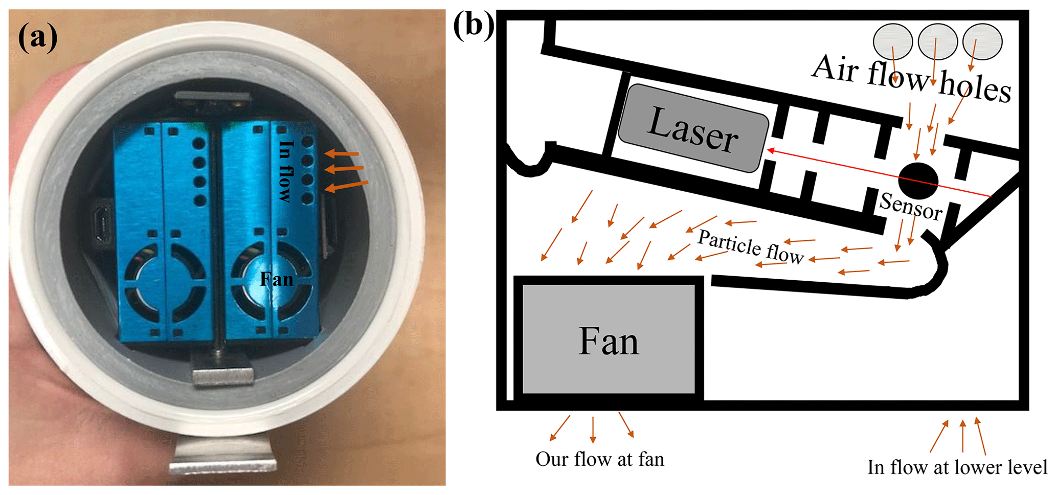
Figure 1(a) Picture from the bottom of the PA-II unit containing two PMS5003 sensors (in blue). (b) Schematic of a single PMS5003 sensor. A fan draws the particles through the inflow (rounded holes) at the lower level of the sensor. The particles travel to the upper part of the sensor where they come out through the air flow holes and then pass through the laser path, causing the beam to scatter. Finally, the particles exit from the fan.
The microcontroller in the PA-II unit reads the PM1.0, PM2.5, and PM10 concentrations from the PMS5003 sensors every second; it averages the concentration values across 20 s and displays the results using UTC time (PurpleAir, personal communication, 2019). The use of a dual PMS5003 sensor setup serves as an internal check for the PA-II unit's integrity. The similarity or difference in the PM concentrations obtained from the two PMS5003 sensors (named A and B) allows users to evaluate the efficiency and validity of their PA-II unit. The two PMS5003 sensors, A and B, should agree with each other at all times; failure to report the same value indicates that something is wrong with one of the sensors. PurpleAir does not calibrate the units; instead, before each PA-II unit is sent out to a customer, the company performs a comparison test with a dozen other PA-II units to find and remove outliers from the shipment (PurpleAir, personal communication, 2019).
All the data regarding the PA-II units and their measurements was downloaded from the PurpleAir website. Information about all the PA-II units was downloaded in a JSON formatted file. Each PA-II unit has a name (given by the owner), a unique ID number (designated by the company for each sensor), the unit location (latitude and longitude), and the date on which the unit was installed. We initially selected all the PA-II units that were active between 1 January 2017 and 31 December 2018 (UTC time). For each selected PA-II unit, we downloaded an Excel file containing the measurement data in 20 s intervals for both PMS5003 sensors (A and B). Because our focus was on PM2.5 measurements, we calculated the PM2.5 hourly average and standard deviation (SD) based on the original measurement values and the daily average and standard deviation based on hourly averages that we had calculated previously. Our final dataset included only days that had a minimum of 13 h of measurements per day (>50 % of the day). Only times that had a good agreement (R2>0.9) of hourly PM2.5 measurements between the two PMS5003 sensors (A and B) were used.
2.2 PM2.5 measurements from AQMS
Hourly measurements of PM2.5 (FRM/FEM Mass code – 88 101 files) from all AQMSs collected by the EPA from 1 January 2017 to 31 December 2018 were selected from the EPA website (https://aqs.epa.gov/api, last access: 1 April 2019). The location of each AQMS was provided in the same file. Each AQMS is identified by the combination of state code, county code, site number, and Parameter Occurrence Code (POC). The POC is used to represent cases in which more than one unit performs PM2.5 measurements at the same site. All timestamps were converted to UTC to match the PA-II measurement timestamps. The PM2.5 daily average and standard deviation were calculated based on the hourly PM2.5 measurements; only days with a minimum of 13 h of measurements per day (>50 % of the day) were considered.
2.3 Identification of locations for analysis – areas with multiple PA-II units and at least one AQMS
By using the JSON file for the PA-II units and the 88 101 file for the AQMS, we calculated the distances between all the units to identify regions with multiple PA-II units (a minimum of five units) and at least one AQMS. At least one AQMS unit needed to be at a distance up to 1.1 km from at least one PA-II unit (defined as a co-located pair, a similar range used by Bi et al., 2020). All the units in these regions needed to be active during the designated time period of 1 January 2017 to 31 December 2018. In each region PA-II units needed to be less than 5 km from at least one AQMS unit and up to 10 km from each other. Four different regions containing a total of seven different AQMSs (all FEM type) and 46 different PA-II units were identified: Denver, CO; San Francisco, CA; Vallejo, CA; and Salt Lake City, UT. Figure 2 shows a map with all the PA-II units and AQMSs at each region. Table S1 in the Supplement provides information on each of the four regions with the names of the units, their locations, first and last times of measurement, and the number of hours measured by each unit. For simplification purposes, each region was defined by two letters to represent its name (DE for Denver, SF for San Francisco, VA for Vallejo, and SL for Salt Lake City). Also, each unit type received a two-letter code (AQ for AQMS and PA for PA-II). Each unit received a number instead of an ID, as shown in Table S1. More than 50 % of the units were at a distance of 4 km from each other. The highest distance between two PA-II units (9.2 km) was in SL. Table S2 lists the distance between each unit per region. The number of concurrent hourly measurements of PA-II units and AQMS units in each comparison varies per region. Overall, the number of concurrent hourly measurements ranged from 95 to 16 658 h with an average of 6412±2924 h. Table S2 lists the number of concurrent PM2.5 hourly measurements between all units in each of the regions.
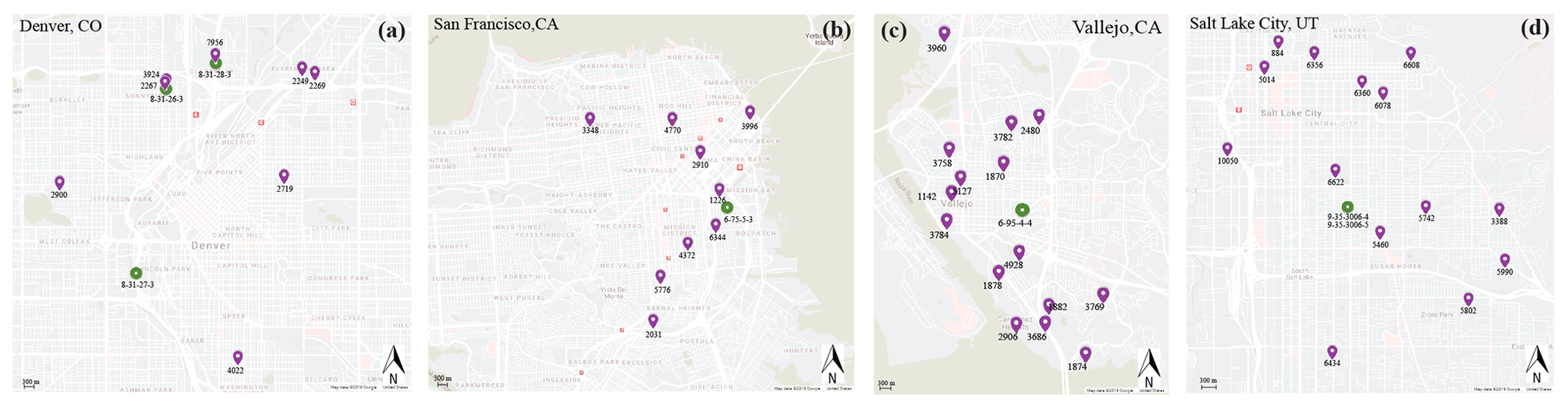
Figure 2Maps of locations with AQMS and PA-II units; each map (a–d) represents a different region: (a) Denver, (b) San Francisco, (c) Vallejo, and Salt Lake City (d). Maps created using © Google maps. AMQS units are represented by the green points, and the PA-II units are represented by the purple points.
To evaluate the similarities and differences between the PA-II units and the AQMSs and other PA-II units, a set of calculations and comparisons was performed using MATLAB and Excel. R-squared (R2), root-mean-square error (RMSE), and mean absolute error (MAE) values, as well as the best fit information (including the slope), were used for the comparison.
2.4 Meteorological information
Meteorological measurements including T, RH, and wind speed and direction were used from the EPA website (https://www.epa.gov/outdoor-air-quality-data, last access: 1 April 2019). Only a few AQMSs had these meteorological measurements: DE-AQ-1, and DE-AQ-3 in Denver, and SL-AQ-1 from Salt Lake City. Additional meteorological measurements such as T, RH, wind speed and gust, wind direction, and visibility of different meteorological stations were obtained from the Iowa Environmental Mesonet website (https://mesonet.agron.iastate.edu/request/download.phtml, last access: 1 April 2019). For meteorological information about the selected regions, the following meteorological stations were used: Denver International Airport (DEN) station, Salt Lake City International Airport (SLC) station, San Francisco International Airport (SFO) station, and the Napa County (APC) station (for Vallejo).
2.5 Remove of outlier PA-II units and irregular hours
The first step was to identify outliers among the PA-II units per region, meaning PA-II units that behave differently from the other PA-II units in their region. By comparing R2 between the PM2.5 values measured by each pair of PA-II units, using a linear regression, we identified the outlier units. A PA-II unit that did not have an R2≥0.75 with at least 75 % of the other PA-II units in its region was considered an outlier unit, and therefore was removed from future analysis (Fig. S1 in the Supplement shows a comparison for each of the four regions). Only one unit from SF (SF-PA-9, see Fig. S1b) had very low R2 when compared to all other PA-II units. Most PA-II units had high R2 values (>0.9) with the other units. Irregular PM2.5 hourly measurements were removed from all units (PA-II and AQMS). These irregular hourly measurements were identified as a large single hourly increase in PM2.5 values (>70 µg m−3) that was not measured by any other unit in the region. Such a large increase was most likely caused by a local source near a specific unit, such as a small-scale fire, lawn mower, barbecue, cigarette smoke, or fireworks (Zheng et al., 2018), and attributed to the location of many of the PA-II units in a residential area. Firework events were removed, as they were very localized events and were measured by a single unit. Overall, less than 0.03 % of the hourly PM2.5 measurements identified as irregular hours were removed from different PA-II and AQMS units.
3.1 Hourly and daily measurements from AQMS and PA-II units
This study examined measurements from a 2-year period from 1 January 2017 to 31 December 2018, resulting in ample overlapping measurement times between the different PA-II units and different AQMSs. Most of the PA-II units became active only at the end of 2017. The frequency of hourly PM2.5 measurements from PA-II units and AQMSs (as well as measurements of RH and T) during the study period in each region were observed to understand the conditions each region had (shown in Fig. S2). Some regions had a high frequency of hourly measurements at low RH (30 %–40 %), while others had high RH (>90 %). Most of the measurements were performed under T of 5–20 ∘C. All regions had a high frequency of PM2.5 between 10–20 µg m−3 for both PA-IIs and AQMSs.

Figure 3Time series of daily PM2.5 measurements from the AQMS and PA-II units in each of the four areas: (a) Denver, (b) San Francisco, (c) Vallejo, and (d) Salt Lake City. Measurements from AQMS are represented by the green lines and the PA-II units are indicated by purple lines.
Time series of daily PM2.5 values for each unit at each of the four regions are presented in Fig. 3. Overall, the daily PM2.5 values obtained from both the AQMSs and the PA-II units seem to follow similar trends. When the AQMS values increase or decrease, the PA-II values also increase or decrease. The PA-II unit measurements of daily PM2.5 values start at 0 µg m−3, and the AQMS can measure negative values owing to its calibration process. In some cases, the AQMS measured higher PM2.5 daily values compared to the PA-II units, mainly on days with low PM2.5 values, as seen in April–June 2018 in Vallejo (Fig. 3c) and Salt Lake City (Fig. 3d). These differences were observed mainly on days with low RH values and low PM2.5 daily values (Fig. S3). However, overall, regardless of the PM2.5 concentration, the PA-II units usually measured higher values compared to those measured by the AQMSs (see July and August 2018 in Denver in Fig. 3a and November 2018 in San Francisco and Vallejo in Fig. 3b and c). This overestimating of PM values by the PA-II units (or PMSs) compared to FRM and FEM units has also been observed in previous studies (Kelly et al., 2017; AQ-SPEC, 2019; Gupta et al., 2018; Sayahi et al., 2019) when the two units were co-located.
The overestimation raises questions about the accuracy of the PA-II units. According to PurpleAir (PurpleAir, personal communication, 2019) the company does not calibrate the PA-II units; instead, before each PA-II unit is sent out to a customer, the company performs a comparison test with a dozen PA-II units to find and remove outliers from the shipment (PurpleAir, personal communication, 2019). Previous studies suggested that part of the problem with the PA-II unit results from the optical particle counter being impacted by changes of RH (Crilley et al., 2018; Malings et al., 2020; Magi et al., 2020). Water vapor can condense on aerosol particles, making them grow hygroscopically under high RH conditions (Lundgren and Cooper, 1969). The PA-II units do not have any heaters or dryers at their inlets to remove water from the sample before measuring the particles; therefore, deliquescent or hygroscopic growth of particles, mainly under high RH conditions, can lead to higher reported PM concentrations (Di Antonio et al., 2018; Jayaratne et al., 2018; Bi et al., 2020), which ends as an overestimate of the PM compared to the reference units. Weather conditions can impact the values reported by low-cost sensors (Morawska et al., 2018). Changes in T or RH have been found to affect the performance of the PA-II units, especially under atmospheric conditions, as they cannot be controlled (Bi et al., 2020). Therefore, MLR between a PA-II and an AQMS, which also considers changes of T and RH, can help correct the reported PM2.5 values of the co-located PA-II units. Similar corrections have been suggested and implemented in other locations with PA-II units (Bi et al., 2020; Magi et al., 2020) and other low-cost sensors (Malings et al., 2020). Most of these studies focus on co-located units or on units that were up to 1 km from the reference unit.
3.2 Correction of PA-II PM2.5 hourly values using a multivariate linear regression
Seven PA-II units were co-located with at least one AQMS unit. In Denver, three PA-II units were co-located with AQMS units. The closest PA-II unit was DE-PA-6, which was only 5.8 m from DE-AQ-3. Unit DE-PA-8 was 30 m from DE-AQ-2, while DE-PA-2 was 79 m from DE-AQ-3. In San Francisco only one PA-II unit was co-located with the AQMS unit. SF-PA-1 was 400 m from SF-AQ-1. In Salt Lake City the two co-located AQMS units (SL-AQ-1 and SL-AQ-2) were 874 m from SL-PA-13. Vallejo unit VA-PA-2 was 1.06 km from VA-AQ-1.
Table 1Details of the coefficients received in each MLR and the linear regression output including R2, RMSE, MAE, and slope for each correction PA-II unit.

Calculations of the ratio between the measured PM2.5 from the PA-II to the AQMS as a function of T and RH, known as a humidogram, were performed (Fig. S4). Some of the PA-II units seem to be impacted by T and RH more than others; these units also had relatively low R2 values with the AQMS unit, as in the case of DE-PA-6 in Denver (Fig. S4a). Only co-located pairs with R2>0.65 were used, reducing the co-located pairs to six. The fact that not all units seem to be impacted in a similar way by the changes of T and RH can explain parts of the debate that exists in the literature. For example, Sayahi et al. (2019) found very low correlation values between measurements from the PMS5003 sensor (used in PA-II) to T and RH under atmospheric conditions. Holstius et al. (2014) found a negligible effect of T or RH on measurements performed using low-cost sensors under ambient conditions. However, several studies that used old PMS units such as PMS1003 which was used in PA-I, or PMS3003 which was never used in any PA units found that these sensors were affected by RH (Kelly et al., 2017; Jayaratne et al., 2018; Zheng et al., 2018). AQ-SPEC (2019) tested the PA-II unit in a laboratory setting under different RH conditions and found that most RH combinations had a minimal effect on the PA-II's precision. On the other hand, Magi et al. (2020) found an impact of T and RH conditions on the PA-II PM2.5 measurements in atmospheric conditions. Therefore, consideration of T and RH was used in the MLR.
An MLR following Magi et al. (2020) was performed on each co-located PA-II and AQMS pair, including meteorological measurements (T and RH). Based on the MLR, the multivariable linear dependence of PA-II PM2.5 on AQMS, RH, and T created the predictors of PA-II as follows:
where A1–A4 fit coefficients received from the MLR, PA-II (PM2.5), and AQMS (PM2.5) are in units of µg m−3; T is in Celsius; and RH is in percentage. Based on these parameters and fit coefficients, a calculation of the corrected PA-II PM2.5 hourly values for each PA-II was performed using the following:
Details of the coefficients received in the MLR, as well as the regression output including R2, RMSE, MAE, and slope for each correction of PM2.5 values in the PA-II units for each region, can be found Table 1. Figure 4 presents a comparison of the PM2.5 values from the uncorrected PA-II unit to the AQMS, as well as the PA-II PM2.5 values hourly after correction, given per region.
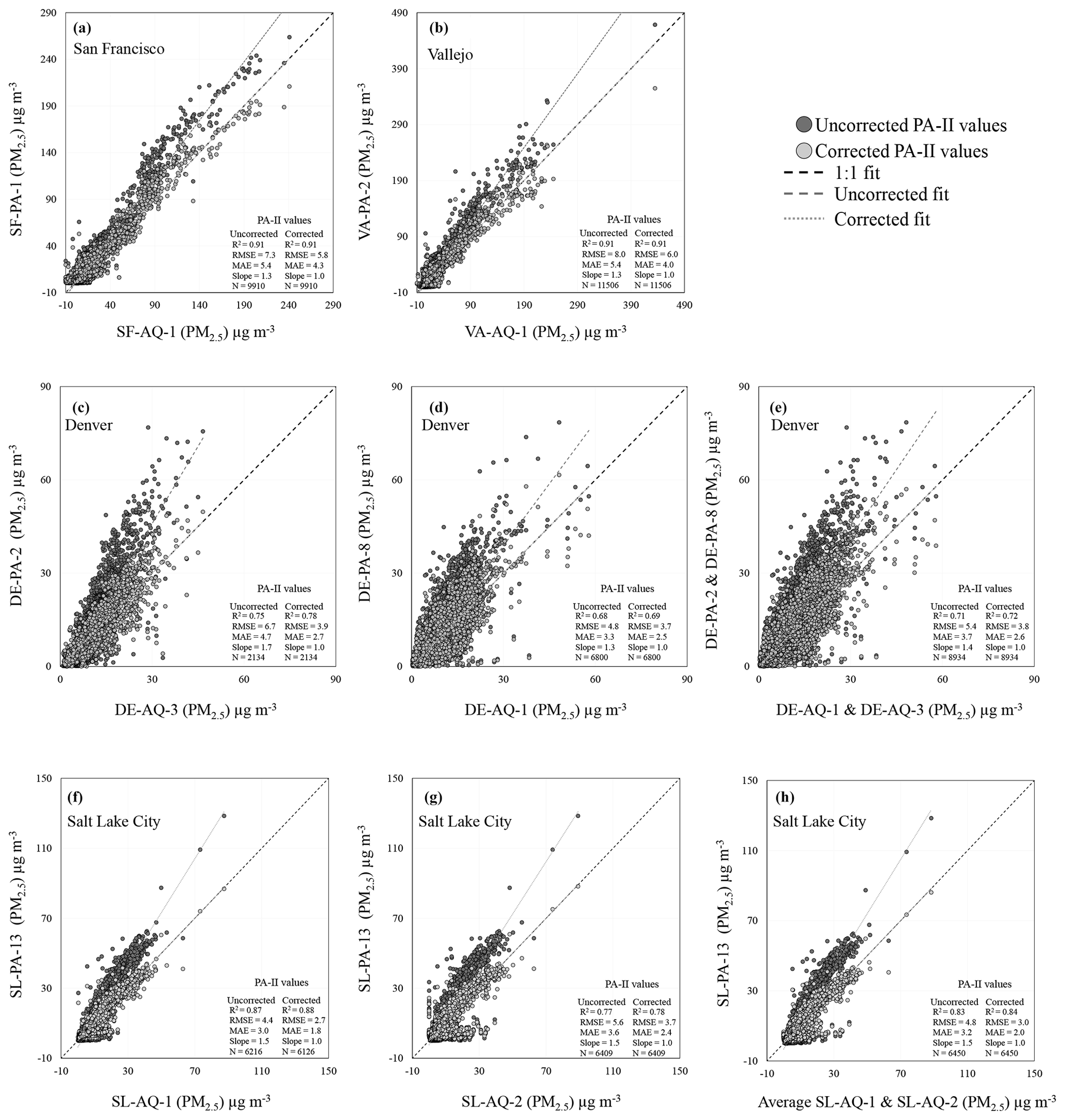
Figure 4Comparison of hourly uncorrected PA-II (PM2.5) values compared to co-located AQMS (PM2.5) values (black) and corrected PA-II (PM2.5) values compared to AQMS (PM2.5) values (gray). Dashed lines represent a 1:1 line. Statistics of each case included the R2, RMSE, and MAE for the uncorrected and corrected (MLR) data. N represents the number of data points used in the MLR for San Francisco (a), Vallejo (b), Denver (c–e), and Salt Lake City (f–h). Different MLR were used from Denver: DE-PA-2 with DE-AQ-3 (c) and DE-PA-8 with DE-AQ-1 (d). New MLR were based on DE-PA-2 with DE-AQ-3 and DE-PA-8 with DE-AQ-1 (e). Different MLR were used for Salt Lake City: SL-PA-13 with SLAQ-1 (f) and SL-PA-13 with SL-AQ-2 (g). New MLR were used based on SL-PA-13 with an average of both AQMS units (h).
3.2.1 Correction of PM2.5 values in co-located PA-II units per region
San Francisco had only one co-located PA-II unit (SF-PA-1) with a single AQMS unit (SF-AQ-1). There were 9910 h of PM2.5 measurements overlapping from both units. The hourly PM2.5 measurements of SF-PA-1 before correction ranged from 0.1 up to 263.8 µg m−3, while SF-AQ-1 ranged from −10 up to 241 µg m−3. Meteorological measurements from the SFO meteorological station, located 16 km from the two units, were used. The meteorological measurements ranged from 0.6 to 33 ∘C for T and 9.2 % up to 100 % for RH. The MLR improved the comparison between SF-AQ-1 and SF-PA-1, as shown in Fig. 4a. While there was no change in the R2 values (0.91), the RMSE and MAE values improved. RMSE decreased from 7.3 µg m−3 before the PM2.5 value corrections to 5.8 µg m−3 after the PM2.5 value corrections, while MAE changed from 5.4 to 4.3 µg m−3. The slope changed with the MLR from 1.3 to 1.0.
Vallejo had one co-located PA-II unit (VA-PA-2) that had 11 506 h of overlapping PM2.5 measurements with VA-AQ-1. The uncorrected PM2.5 measurements from the PA-II unit ranged from 0 up to 468.5 µg m−3, while AQMS PM2.5 measurements ranged from −10 up to 435 µg m−3. The meteorological station that was used for this PA-II PM2.5 value correction (APC) was 11 km away from the AQMS. The meteorological measurements during this comparison ranged from −5 to 41 ∘C and 5.8 % up to 100 % for T and RH, respectively. The MLR improved the comparison between the PA-II and the AQMS (Fig. 4b). There was no change in the R2 values, which was 0.91, yet RMSE and MAE values decreased. RMSE decreased from 8.0 to 6.0 µg m−3, while MAE decreased from 5.4 µg m−3 before the PM2.5values corrections to 4.0 µg m−3 after the PM2.5 value corrections. The slope also improved from 1.3 to 1.0.
Denver had two different PA-II units that were co-located with two different AQMS units. Unit DE-PA-8 had 2134 h of overlapping PM2.5 measurements with DE-AQ-2, while DE-PA-2 had 6800 h of overlapping PM2.5 measurements with DE-AQ-3. The range of the PM2.5 values were similar for both PA-II units. DE-PA-2 ranged from 0.1 up to 76.9 µg m−3, while DE-PA-8 ranged from 0.1 up to 78.5. The AQMS units also had relatively similar PM2.5 measurements, which ranged from 0.3 up to 57.9 µg m−3 for DE-AQ-2 and from 0.9 up to 46.6 µg m−3 for DE-AQ-3. Both AQMS units had meteorological measurements as part of the AQMS units that were used for the MLR. Temperature measurements for DE-PA-2 ranged from −9.4 up to 39.4 ∘C, while DE-PA-8 T measurements ranged from −5.6 up to 34.4 ∘C. RH measurements were very similar as well, ranging from 3 % for DE-PA-2 and 4 % for DE-PA-3 and up to 98 % for both. Although there were similar ranges of PM2.5, T and RH measurements were taken, and there were differences between the PA-II's comparison to their co-located AQMS units. DE-PA-2 had better correlation values before and after the MLR (R2 of 0.75 and 0.78, respectively) compared to DE-PA-8 (R2 of 0.68 and 0.69, respectively; see Fig. 4d). RMSE and MAE values for both cases improved by more than 1.1 µg m−3 for the RMSE and 0.8 µg m−3 for the MAE. The slope values, which were 1.7 and 1.3 before the MLR, reduced to 1.0 in both cases. While the DE-PA-2 with DE-AQ-3 had higher R2 values, it also had higher RMSE and MAE values compared to the DE-PA-8 and DE-AQ-1 pair. The two co-located pairs were combined and compared before and after the MLR (Fig. 4e). R2, RMSE, and MAE values were in the same range in the two separate comparisons. R2 improved from 0.71 to 0.72 before and after the MLR, respectively. RMSE changed from 5.4 to 3.8 µg m−3, and MAE changed from 3.7 to 2.6 µg m−3. The value of the slope also improved from 1.4 to 1.0 after the correction of PA-II PM2.5 values. The combined MLR had a higher number of observations and R2, RMSE, and MAE values that were in the range of each of the separate comparisons.
The last region with co-located units was Salt Lake City. In this region one PA-II unit (SL-AP-13) was co-located with two AQMS units that were in the same location (SL-AQ-1 and SL-AQ-2). Measurements of T and RH were used from SL-AQ-1 meteorological station. SL-AQ-1 had 6216 h of overlapping PM2.5 hourly measurements with SL-AP-13, while SL-AQ-2 had slightly more overlapping measurements (6409 h). The meteorological parameters during these comparisons ranged from −7.2 to 38.3 ∘C for T and 2 % up to 91 % for RH. The uncorrected PM2.5 measurements from the PA-II unit ranged from 0 up to 128.5 µg m−3, while the PM2.5 measurements ranged from 0.1 up to 87.5 µg m−3 for SL-AQ-1 and 0.1 up to 89.1 µg m−3 for SL-AQ-2. We first evaluated the MLR for each of the AQMS units separately (Fig. 4f and g). Different R2, RMSE, and MAE values were obtained. While both showed an improvement of the RMSE, MAE, and slope value after the PM2.5 value corrections, the MLR with SL-AQ-1 had better results with a higher R2 (0.88 compared to 0.78) and lower RMSE (2.7 µg m−3 compared to 3.7 µg m−3) and MAE (1.8 µg m−3 compared to 2.4 µg m−3) values. Combining the hourly PM2.5 values from the two AQMSs together, since both were in the same location, was performed by averaging the AQMS PM2.5 values (Fig. 4h). The MLR results showed an increase in R2 and a decrease in RMSE and MAE values. Averaging of the AQMS units provided lower RMSE and MAE values and higher R2 values compared to one of the separate options. This MLR had low RMSE and MAE values (3.0 and 2.0 µg m−3, respectively) and a high R2 (0.84) value, making this MLR better than the one used by the pair SL-PA-13 with SL-AQ-2.
3.2.2 Corrections of PA-II PM2.5 values of other PA-II units per region based on MLR
Based on the different coefficient values received in each MLR (Table 1), we implemented Eq. (2) on each of the uncorrected PA-II units' PM2.5 hourly values, using the same meteorological parameter used for the MLR corrections. San Francisco and Vallejo each only had one set of comparisons and coefficients, while there were several options for Denver and Salt Lake City. The new PM2.5 hourly values (corrected) from each PA-II unit were compared to the nearest AQMS unit and to all the other PA-IIs in the region using a linear regression. Corrected PM2.5 hourly values of PA-II unit measurements improved the comparison between the other PA-IIs and AQMS units, as shown by the general reduction of RMSE, MAE, and the slope. Figure 5 shows comparison to AQMSs. See Table S3 for the full details of all comparison results.
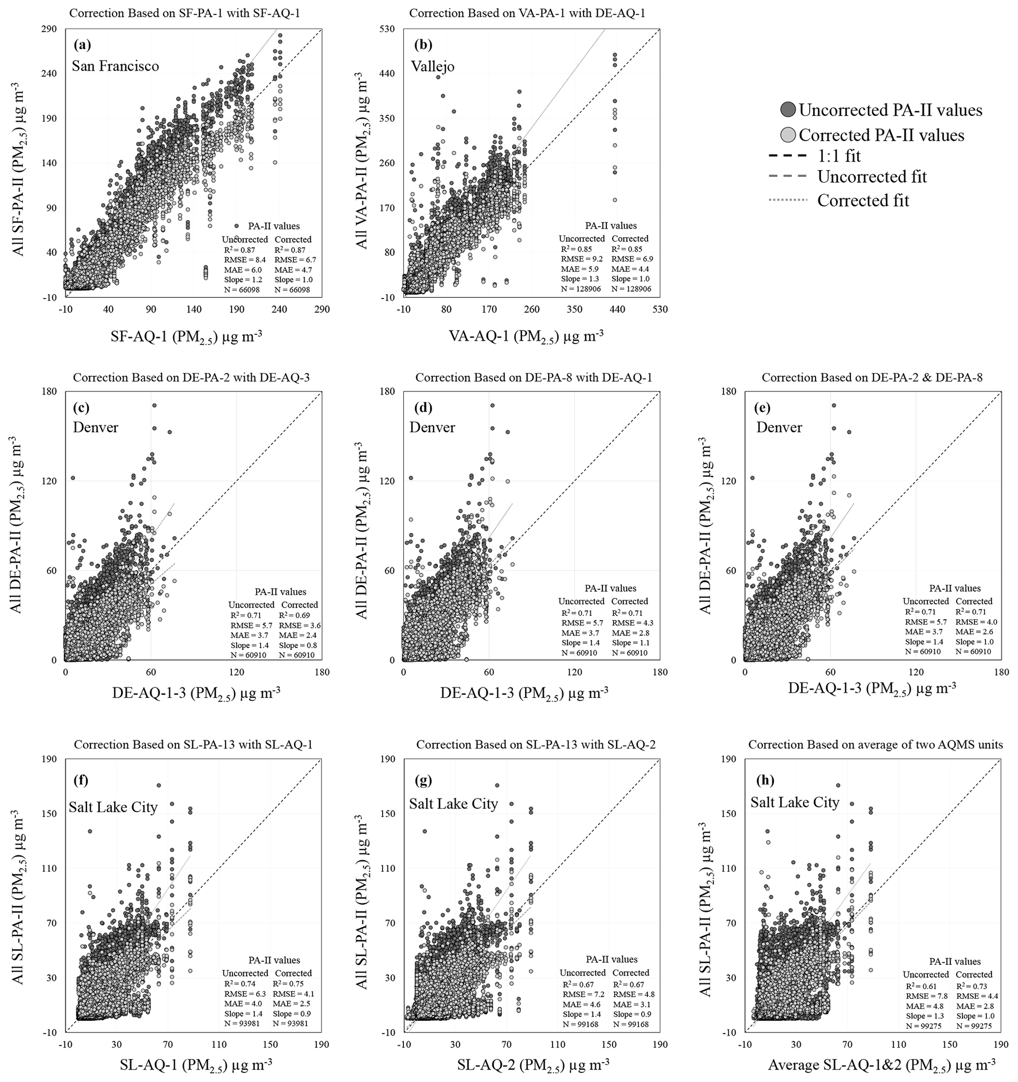
Figure 5Comparison of hourly uncorrected PA-II (PM2.5) values compared to nearest AQMS (PM2.5) values (black) and corrected PA-II (PM2.5) values compared to AQMS (PM2.5) values (gray). Dashed lines represent a 1:1 line. Statistics of each case included the R2, RMSE, and MAE for the uncorrected and corrected (MLR) data. N represents the number of data points used in the MLR. Each figure represents corrections based on different MLR type: San Francisco (a) based on SF-PA-1 with SF-AQ-1 and Vallejo (b) based on VA-PA-1 with DE-AQ-1. Different corrections were made for Denver (c–e): DE-PA-2 with DE-AQ-3 (c) and DE-PA-8 with DE-AQ-1 (d) and combining DE-PA-2 with DE-AQ-3 and DE-PA-8 with DE-AQ-1 (e). Different corrections were made for Salt Lake City (f–h): based on SL-PA-13 with SL-AQ-1 (f) and SL-PA-13 with SL-AQ-2 (g), and the MLR was based on SL-PA-13 with an average of both AQMS units (h).
The comparison of each unit in San Francisco and Vallejo before and after implementing the PA-II PM2.5 value corrections did not change the R2 values between the PA-IIs and AQMS units (Table S3a and b). The average R2 value between the PA-IIs and AQMS units for Vallejo was 0.79±0.13, while San Francisco's average R2 value was 0.83±0.11. No changes were observed among the comparison of the PA-IIs themselves (0.93±0.06 for San Francisco and 0.89±0.07 for Vallejo). However, reductions in RMSE and MAE values were observed in both regions (see Fig. 5a for San Francisco and Fig. 5a for Vallejo).
The average RMSE values for San Francisco for the PA-IIs with the AQMSs changed from 8.23±0.66 to 6.53±0.54 µg m−3. Similar improvements were observed when the PA-II units were compared to the other PA-II units; average RMSE changed from 4.23±1.05 to 3.39±0.83 µg m−3. Similar reductions were also observed for the MAE; average MAE values for the PA-IIs with the AQMSs changed from 5.84±0.31 to 4.61±0.26 µg m−3. Even when the PA-IIs were compared to the other PA-II units, a reduction in MAE was observed; the average MAE changed from 2.16±0.35 to 1.71±0.28 µg m−3. A reduction was also observed in the average slope value (Table S3a).
Vallejo also had a reduction in RMSE and MAE values after the MLR. The average RMSE values for the PA-II with the AQMS changed from 8.95±1.35 to 6.73±1.05 µg m−3. Similar improvements were observed when the PA-II units were compared to the other PA-II units. RMSE changed from 5.14±1.48 µg m−3 before the PM2.5 value corrections to 3.89±1.12 µg m−3 after the PA-II PM2.5 value corrections. Similar reductions were also observed for the MAE; average MAE values for the PA-II with the AQMS changed from 5.81±0.61 to 4.33±0.46 µg m−3. Even when the PA-IIs were compared to the other PA-II units, a reduction in MAE was observed; the average MAE changed from 2.5±0.56 to 1.89±0.42 µg m−3. A reduction was also observed in the average slope value (Table S3b).
In Denver three different correction options were evaluated based on two separate pairs of PA-IIs with AQMSs and a combination of both together. Since there were several AQMS units, each PA-II unit was compared to its nearest AQMS unit (see Table S2a for distances, the distances ranged from 0 to 4 km). The coefficient values were different between each MLR option (Table 1). The R2, RMSE, MAE, and slope were very similar (Fig. 5c–e). No change in R2 was observed in each MLR type. A reduction in RMSE was observed after the PA-II PM2.5 values were corrected. The average RMSE value, between each PA-II to the nearest AQMS unit, before the correction, was 5.7±0.8 µg m−3. All three correction types had lower average RMSE values. Correction of PA-II PM2.5 values based on DE-PA-2 with DE-AQ-3 had an average RMSE value of 3.6±0.3 µg m−3, lower than the average RMSE from the corrections that were based on DE-PA-8 with DE-AQ-1 (4.3±0.5 µg m−3). The correction that combined both units had an average RMSE in the range of the two correction options (4.0±0.5 µg m−3). Similar reduction trends were observed for the MAE values. The average MAE values between each PA-II to the nearest AQMS unit, before the PA-II PM2.5 value corrections, was 3.8±0.6 µg m−3. Correction of PA-II PM2.5 values based on DE-PA-2 with DE-AQ-3 had an average MAE value of 2.4±0.2 µg m−3, lower than the average MAE based on DE-PA-8 with DE-AQ-1 (2.8±0.4 µg m−3). Yet the combined option had MAE in the range of the other two (average of 2.6±0.3 µg m−3). Reductions of RMSE and MAE were observed when the PA-II units were compared to the other PA-II units (Table S3c). The average RMSE and MAE values between all PA-II units before the correction were 3.9±1.0, and 2.4±0.6 µg m−3, respectively; after the corrections of PA-II PM2.5 both RMSE and MAE values decreased. Correction of PA-II PM2.5 values based on DE-PA-2 with DE-AQ-3 had average RMSE and MAE values of 2.4±0.6 and 1.5±0.4 µg m−3, respectively. These values were lower than those that were based on the correction type of DE-PA-8 with DE-AQ-1 (average RMSE was 3.0±0.7 µg m−3, while the average MAE was 1.8±0.5 µg m−3). The PA-II PM2.5 value corrections that combined both units had average RMSE and MAE values in the range of the two correction options.
Three different options of PA-II PM2.5 value corrections were performed in Salt Lake City, one of SL-AP-13 with each of the two AQMS units (SL-AQ-1 and SL-AQ-2) and another after the PM2.5 values of the AQMS units were averaged. The corrections of the PA-II (PM2.5 values) units in Salt Lake City varied depending on the type of corrections and coefficient used. While all options of PA-II PM2.5 value corrections improved the comparison between the PA-II to the AQMS units and between the PA-II themselves (Fig. 5f–h, Table S3d), there was no significant change in the R2 values when the PA-II units were compared to the AQMSs. Overall corrections of PA-II PM2.5 values based on SL-AQ-2 had lower R2 values and higher RMSE and MAE values compared to the other two correction options. The average RMSE between the PA-II and the AQMS units based on SL-AQ-1 MLR was 6.0±1.2 µg m−3. After the PA-II PM2.5 value corrections the average RMSE reduced to 3.8±0.7 µg m−3. A reduction was also observed for the average MAE value, which changed from 3.7±0.8 to 2.3±0.5 µg m−3 after implementing the SL-AQ-1 MLR. Reductions of RMSE and MAE values were also observed when the PA-II PM2.5 value corrections were based on averaging the PM2.5 values from both AQMS units. The average RMSE between the PA-II and the AQMS units was 6.1±0.9 µg m−3 before the correction of PA-II PM2.5values and 3.9±0.6 µg m−3 after the correction of PA-II PM2.5 values. A reduction was also observed for the average MAE value, which changed from 3.8±0.7 to 2.5±0.4 µg m−3 after implementing the average AQMS option. A reduction of RMSE and MAE was also observed when the PA-II units were compared to other PA-II units. Before the PA-II PM2.5 value corrections, the average RMSE and MAE values were 4.4±1.7 and 2.24±0.96 µg m−3, respectively. After the corrections of PA-II PM2.5 values with SL-AQ-1, the average RMSE and MAE values were reduced to 2.65±0.98 and 1.44±0.62 µg m−3, respectively. Similar values were found for the PA-II PM2.5 value corrections that were based on average AQMSs. The average RMSE and MAE values after the PA-II PM2.5 value corrections were 2.64±0.97 and 1.43±0.62 µg m−3, respectively.
Overall, almost all the PA-II units had high correlation values when compared with the other PA-IIs or AQMSs in their region. Two PA-II units, SL-PA-6 and SL-PA-8, had low R2 values with the AQMS, and they also had a relatively low correlation with the other PA-II units. It is feasible that if stricter rules for identifying outlier PA-II units were in use, these two units would have been considered as such and subsequently removed from the dataset.
Although improvements of RMSE, MAE, and slope values were observed for the entire research time period, the comparison only provides a general overview on the units' behaviors but cannot provide information on the variability of the PM2.5 values under different conditions mainly under high-pollution events. Therefore, in order to evaluate whether the PA-II PM2.5 value corrections improved the performance of PA-II units, a comparison of PM2.5 values at different locations that experienced similar meteorological conditions or pollution types needed to be performed.
3.3 Comparison of PA-II units in high-pollution events
Observations of the PA-II units under high-pollution conditions were performed based on daily measurements of PM2.5 values from different regions that experienced different pollution types. It is known that different meteorological conditions, such as wind direction or speed and pollution type (traffic, industrial, wildfire, etc.) or source (local vs. regional), may affect the comparison between the AQMSs and the PA-II units. We aimed to determine how the PA-II units behaved (before and after PA-II PM2.5 value corrections) in a high-pollution event when the daily PM2.5 concentration exceeded the EPA daily regulation of 35 µg m−3. Therefore, we investigated specific events with high PM2.5 concentrations in different time frames under different atmospheric conditions in each region included in this study.
3.3.1 Wildfire in California
The two studied regions in California, Vallejo and San Francisco, are relatively close to each other, and both were affected by a large wildfire that occurred in November 2018. According to the California statewide wildfire recovery resources (2019), the wildfire started on 8 November in Butte County (north of Vallejo) owing to a combination of strong winds and very dry conditions. A southwesterly wind transferred the wildfire smoke from Butte County toward Vallejo and San Francisco. Very high daily PM2.5 values were measured from 9 to 21 November (Fig. 6a and b). During this period, the area had stable meteorological conditions, with low wind speed that reduced visibility down to 1.6 km (1 mile). The high daily PM2.5 values decreased only after precipitation started on November 21. Overall, in each of the regions, the values measured by the PA-II units increased at the same time and followed a similar trend to the AQMS measurements. A comparison of the PM2.5 values measured by the PA-IIs before and after the correction (Fig. 6a and b) showed that the measured (uncorrected) PA-II PM2.5 values were higher compared to the AQMS values. In San Francisco, during the wildfire days, the PA-II measured on average 30.3±13.2 µg m−3 higher PM2.5 daily values than the AQMS. Similar values were also found for Vallejo (30.2±13.0 µg m−3). However, after the correction of PA-II PM2.5 values, the daily PM2.5 values were lower than before, and they were in a similar range to those measured by the AQMS units. The corrected PA-II PM2.5 daily values during the wildfire were still slightly higher than those measured by the AQMS during the same time. In San Francisco the corrected PM2.5 daily values were on average 6.7±12.0 µg m−3 higher than those measured by the AQMS. Lower values were found for Vallejo (1.7±11.8 µg m−3). However, a closer look at the daily values in each of the two regions found that, after the correction of PA-II PM2.5 values for specific daily values that exceeded 100 µg m−3, the daily values of the corrected PA-IIs were lower than the daily PM2.5 values measured by the AQMS. During one such day the corrected PA-II PM2.5 daily values were lower by 29 µg m−3 compared to the daily PM2.5 value measured by the AQMS. The underestimation may be a result of not having enough hourly measurements with such high PM2.5 values. Both regions had very low number of hours with PM2.5>100 µg m−3; only 0.15 % of the hourly measurements in San Francisco had PM2.5 hourly measurements from the AQMS that exceed 100 µg m−3. Vallejo had a lower value of 0.1 %. Therefore, there were not enough data points to train the MLR model, which resulted in lower PA-II values.

Figure 6Daily measurements of PM2.5 at (a) San Francisco and (b) Vallejo during the November 2018 wildfire (UTC time). Daily PM2.5 measurements at Salt Lake City during 1–14 December 2018 during inversion (c). Daily PM2.5 measurements at Denver during haze, 1–15 September 2017 (d). Each location shows measurements before the PA-II PM2.5 measurements were corrected and after each of the correction options. AMQS units are represented by the different green lines and the PA-II units are represented by the different purple lines. Bars represent the standard deviation per day values.
3.3.2 Inversion in Utah
In Utah, Salt Lake City had higher daily PM2.5 values during 4–13 December 2018 (Fig. 6c). The entire area was affected by an inversion for several days (3–13 December), which increased the daily PM2.5 values and reduced the visibility to almost zero (see photos in Williams, 2019). Overall, the values measured by the PA-II units increased at the same time and followed a similar trend to the AQMS measurements. However, whereas all the PA-II units measured similar PM2.5 values, uncorrected PM2.5 daily values from the PA-II during these days were much higher than those measured by the AQMS (on average 9.2±7.4 µg m−3 more each day). PM2.5 values only decreased after precipitation occurred on 13 December. There were three corrections of PA-II PM2.5 values for the PA-II units in Salt Lake City. After each of the PA-II PM2.5 value corrections, the corrected PM2.5 daily values seemed to be similar to those measured by the AQMS units (Fig. 6c). The average daily concentration during these days was slightly higher. Both PA-II PM2.5 value corrections of PA-II values that were based on SL-PA-13 with SL-AQ-2 or SL-AQ-1 had higher concentrations compared to the AQMS; on average the PA-II daily average during these days was higher by 1.7±2.4 µg m−3 for SL-PA-13 with SL-AQ-1 and by 1.7±2.5 µg m−3 for SL-PA-13 with SL-AQ-2. The PA-II PM2.5 value corrections that used averaged AQMS values had slightly higher PM2.5 daily values. On average the PA-II values were higher by 2.1±2.6 µg m−3 from those measured by the AQMS. The still higher PM2.5 values could be due to the volatility of ammonium nitrate, which is a dominant aerosol composition at the region of Salt Lake City during the winter times (Moravek et al., 2019; Womack et al., 2019). It has been shown that sensors similar to the ones used in the PA-II units would be less likely to volatilize ammonium nitrate, unlike the one used in the AQMS units (Grover et al., 2005).
3.3.3 Haze in Denver
On 4 September 2017, a thick hazy smoke from western wildfires settled into eastern Colorado (Spears, 2020). Haze was reported by the DEN meteorological station from 06:00 UTC until the end of the day. Low wind speeds (average of 3.7±0.9 m min−1 until 20:00) were recorded and visibility was reduced to 4 km (2.5 miles). Visibility started to increase only around 22:00 UTC. PM2.5 daily measurements from AQMS units in Denver during this day increased up to 37.1 µg m−3. Before the PA-II PM2.5 value corrections, PM2.5 daily measurements from the four PA-II units that were active during this period were almost double (the average concentration of the four units was 69.3±2.1 µg m−3). The PM2.5 daily measurements from the four PA-II units were higher than those taken by the AQMS units for almost the entire duration of 1–11 September but lower than the remaining days (Fig. 6d). On average the PA-IIs measured 8.3 µg m−3 more PM2.5 daily concentration than the AQMS units during the entire period. There were three PA-II PM2.5 value-correction options in this area, two were based on two different co-located PA-II and AQMS units, and another combined these two pairs. All PA-II PM2.5 value corrections showed a reduction in the daily PM2.5 values compared to the measured (uncorrected) case, yet the corrected daily PM2.5 values were higher for almost this entire period. On average, the corrected PA-II PM2.5 values were 1.2 µg m−3 higher than the AQMS values (during this entire period) when the PA-II PM2.5 values were corrected based on DE-PA-2 with DE-AQ-3. Higher values were calculated in the other two PA-II PM2.5 value-correction types (3.5 and 2.8 µg m−3 based on DE-PA-8 with DE-AQ-1) and the one type that combined both co-located pairs.
3.4 Impact of distance on comparisons between the units
Previous studies obtained good results when comparing the PA-II unit or PMS5003 sensor and the FRM and FEM units when the two units were co-located. The AQ-SPEC (2019) recently released a report comparing PA-II units to two FEM instruments under laboratory and field conditions. They found good correlations for hourly and daily values of both PM2.5 and PM10 under field conditions, with higher correlation values for PM2.5 compared to those for PM10. Gupta et al. (2018) compared three PA-II units in California to a single FEM unit and obtained good correlation values (R2>0.9). Sayahi et al. (2019) co-located reference air monitors (tapered-element oscillating microbalance, TEOM) and an FRM unit next to a PMS5003 (used in the PA-II unit) in Salt Lake City. The PMS5003 PM2.5 measurements correlated well with the hourly TEOM measurements (R2>0.87) and with the daily FRM measurements (R2>0.88). In our study, we did not position the PA-II units. Further, in most cases, the AQMS and the PA-II units were not co-located; therefore, they might have been exposed to different particle types and concentrations. Some might claim that not having the PA-II and FRM units co-located, as was done in previous studies, might diminish the accuracy of the comparison between these units. Although lower correlation values were in fact observed in our study, as we were using PA-II units in their natural locations, this was expected. Further, as we saw that the correlation values are not much lower than those in the co-located cases described in previous studies, they are still statistically significant. Because the AQMS and the PA-II units were not co-located, we wanted to verify whether the distance between all the units affected the R2, RMSE, MAE, and slope values. We compared the R2, RMSE, MAE, and slope values received from the comparisons of hourly PM2.5 measurements with the corresponding distances between the units (Fig. 7). There was no correlation between the two when the PA-II units were compared to the nearest AQMS units (Fig. 7a) or between the PA-II units (Fig. 7b), before or after the corrections of the PA-II PM2.5 values. Therefore, the distance between the units did not impact the comparison.

Figure 7Comparison of distance (km) between PA-II and its nearest AQMS in all regions (a) and between each PA-II unit and all other PA-II units per region (b) for R2, RMSE, MAE, and slope values received from the PM2.5 hourly measurements comparison.
3.5 Underlying differences and future implications
While appropriate PA-II PM2.5 value corrections can improve comparison between the PA-IIs with reference units, there are other differences between PA-IIs and AQMS units that can influence the comparison results, including the underlying technology and the manner in which units are placed. The PM2.5 sensors in the AQMSs perform gravimetric measurements using the mass of the particle; by contrast, the PA-II units use a laser particle counter to count electric pulses generated as particles crossing through a laser beam. The method used by the PA-II might impact the count of particles during high-humidity conditions or when a majority of the particles are volatile. Another difference is the physical location of the units; whereas AQMSs are meticulously positioned in an open area, the location of a PA-II is determined by its owner. Although PurpleAir recommends positioning the PA-II in an open area, ultimately it is the owner's decision. In practice, most of the PA-II units are located in residential areas with low-rise housing. Furthermore, the height at which the sensor is located could affect the measurements. The height of the AQMS inlet is regulated and kept constant at each location; on the other hand, the owner of a PA-II unit can freely place it near the ground or higher up. The location of the PA-II units in residential areas can provide both an advantage and a disadvantage. For example, a single PA-II unit might be exposed to more localized PM sources such as a barbecue, lawn mower, or car, making it report different results when compared with other units in its area. Therefore, an increase in PM by a single PA-II unit should be taken into account. When the PA-II is used as a network, as suggested by Ford et al. (2019), comparison of the PM values measured by all PA-II units will help identify such a localized source. Maintenance and calibration are other possible causes of differences between the two. The PM2.5 sensors in the AQMSs have strict rules for the monthly evaluation of sensor performance, including through flow calibration or calibration based on a minimum value threshold (which, in some cases, causes the recording of negative PM values). By contrast, PA-II units do not have any quality control other than that done by the company for each sensor before shipment to the customer (PurpleAir personal communication, 2019). Another point that should be taken into account is the lifetime of the PA-II units. The manufacturer of the PMS5003 sensor used in the PA-II units states that it has a lifetime expectancy of ∼3 years (Yong, 2018). Bi et al. (2020) found that the PA-II unit's efficiency is affected even after only 2 years of being operational.
Based on the findings from this work, we believe that there are several needed steps that will allow the usage of the PA-II units in air-quality- and health-related research. First, users should identify regions with multiple PA-II units where at least one PA-II is co-located with an FRM or FEM unit. Ideally the same location will also contain measurements of T and RH or at least T and RH measurements will be nearby. Keep in mind that it is not recommended to use the PA-II internal sensors for T and RH values, as they do not represent the atmospheric measurements (Malinges et al., 2020; PurpleAir, personal communication, 2019). However, we have found that in many regions there is no meteorological station that can serve as a reference for the correction process. It would be useful then to devise a way in which the PA-II internal T and RH sensors can be used. To achieve this, an extensive study is necessary to gain a better understanding of the issues related to the usage of the PA-II internal sensors and to formulate a calibration equation that then can be applied to the desired PA-II units.
Comparison of all PA-II units in each region will help to identify and remove outlier PA-II units from future analysis. Exposure to high PM concentration might affect the PA-II efficiency, as suggested by Sayahi et al. (2019), and therefore its measurements will differ substantially from those of the AQMSs and other PA-II units. Ideally PurpleAir should monitor all active PA-II units, identify units that behave differently from surrounding PA-II units or PA-II units whose internal sensors (A and B) report different values, flag them on the online map, and communicate instructions to the unit owners on how to fix or replace the unit.
After PA-II units have been identified, users should conduct MLR between the co-located PA-II and AQMS units, including measurements of T and RH. For the MLR to be efficient it is important have a wide range of PM2.5, T, and RH measurements. This MLR will provide a coefficient that will be used to correct all the remaining PM2.5 values of all PA-II units in that region. Evaluation of the PA-II PM2.5 value corrections should be made for the duration of the study but also for specific events with spatial impact such as inversion, dust storms, biomass burning, and more. Such events should impact a larger area and therefore will allow detection of the PM changes in all PA-II units as a whole (network). Correction of PA-II PM2.5 values should be performed per region, as they represent specific PM values and changes of T and RH values that the PA-II units were exposed to. This will help the public obtain information on the spatial and temporal distribution of PM concentrations in their area (Gupta et al., 2018; Morawska et al., 2018), which will enable them to monitor local air quality conditions (Williams et al., 2018) and help make decisions related to events with high PM exposure.
In this study, we evaluated PA-II units that were up to 5 km away from an AQMS unit, as well as up to 10 km from each other. This raises the question of maximum effective distance. What is the maximum distance between an AQMS and PA-II units that will still allow for the MLR to successfully correct the measurement taken by PA-II units; a distance greater than this would carry the potential of introducing additional factors that might impact the comparisons. Another situation that requires further investigation is that of regions that include multiple PA-II units but do not have a co-located pair or completely lack a reference monitoring station. The question in mind is (if possible) how we might use neighboring regions in which measurements were successfully corrected to compensate in the case of such problematic areas. For example, could we have used Vallejo and San Francisco, two regions that were included in this study, to correct the measurements of the PA-II units in the region of Berkeley–Oakland that resides between the two?
PA-II units are becoming a common low-cost tool to monitor changes in the concentrations of PMs of various sizes. Previous studies have examined the performance of these PA-II units (or the sensor in them) by comparing them with a co-located EPA AQMS. However, a majority of PA-II units are not co-located in practice, and some of them are placed in areas where there is no reference air monitoring system. This study aimed to examine the behavior of PA-II units under atmospheric conditions when exposed to a variety of pollutants and different PM2.5 concentrations. For this purpose, we used PA-II units that have already been active for some time, irrespective of where they might be located. Four regions with multiple PA-II units and at least a single AQMS were identified. Each region had at least one co-located pair of a PA-II with an AQMS. Corrections of PA-II PM2.5 values using MLR based on the AQMSs' PM2.5, RH, and T values of these co-located units improved the comparison of the PA-II (co-located and not co-located) with the AQMS unit (higher R2, lower RMSE and MAE, and better slope values). Overall, the PA-II units behaved in a similar way to the other PA-II units in their regions. Without corrections of PA-II PM2.5 values, the majority of PA-II units measured much higher values than the AQMSs. After corrections of PA-II PM2.5 values, PA-II units were in agreement and measured overall similar PM2.5 concentrations. We think that the PA-II unit is a promising tool for measuring PM2.5 concentrations and identifying relative concentration changes, as long as the PA-II PM2.5 values can be corrected.
Data will be provided by the authors upon request.
The supplement related to this article is available online at: https://doi.org/10.5194/amt-13-5441-2020-supplement.
KAD designed the study, supervised it, and performed most of the analysis. YD wrote the MATLAB code that was used for all stages of the analysis and for the figure creation. NM was responsible for several sections of data analysis and figures. JW participated in the data analysis. KAD and YD wrote the manuscript. All authors were actively involved in interpreting results and in discussions about the manuscript.
The authors declare that they have no conflict of interest.
The authors are thankful to the PurpleAir team for their help and explanations about the PA-II units. Further, they are thankful to Mangus Nick from the National Air Data Group at the US EPA for his help with the EPA data. Finally, they are thankful to Amber McCord, from the College of Media & Communication at Texas Tech University, for her help with the Key Figure. Use of the sensor manufacturer's name does not imply endorsement.
This paper was edited by Francis Pope and reviewed by two anonymous referees.
AQ-SPEC – the Air Quality Sensor Performance Evaluation Center: PurpleAir PA-II evaluation summary, available at: http://www.aqmd.gov/docs/default-source/aq-spec/summary/purpleair-pa-ii---summary-report.pdf?sfvrsn=4, last access: 1 August 2019.
Bi, J., Wildani, A., Chang, H. H., and Liu, Y.: Incorporating Low-Cost Sensor Measurements into High-Resolution PM2.5 Modeling at a Large Spatial Scale, Environ. Sci. Technol., 54, 2152–2162, https://doi.org/10.1021/acs.est.9b06046, 2020.
California wildfires statewide recovery resources: November 2018 Fires, available at: http://wildfirerecovery.org/general-info/, last access: 21 June 2019.
Castell, N., Dauge, F. R., Schneider, P., Vogt, M., Lerner, U., Fishbain, B., Broday, D., and Bartonova, A.: Can commercial low-cost sensor platforms contribute to air quality monitoring and exposure estimates?, Environ. Int., 99, 293–302, 2017.
Clements, A., Griswold, W. R. S. A., Johnston, J. E., Herting, M. M., Thorson, J., Collier-Oxandale, A., and Hannigan, M.: Low cost air quality monitoring tools: from research to practice (a workshop summary), Sensors, 17, 2478, https://doi.org/10.3390/s17112478, 2017.
Cohen, A. J., Brauer, M., Burnett, R., Anderson, H. R., Frostad, J., Estep, K., Balakrishnan, K., Brunekreef, B., Dandona, L., Dandona, R., Feigin, V., Freedman, G., Hubbell, B., Jobling, A., Kan, H., Knibbs, L., Liu, Y., Martin, R., Morawska, L., Pope,C. A., Shin, H., Straif, K., Shaddick, G., Thomas, M., van Dingenen, R., van Donkelaar, A., Vos, T., Murray, C. J. L., and Forouzanfar, M. H.: Estimates and 25-year trends of the global burden of disease attributable to ambient air pollution: an analysis of data from the Global Burden of Diseases Study 2015, Lancet, 389, 1907–1918, https://doi.org/10.1016/S0140-6736(17)30505-6, 2017.
Commodore, A., Wilson, S., Muhammad, O., Svendsen, E., and Pearce, J.: Community-based participatory research for the study of air pollution: a review of motivations, approaches, and outcomes, Environ. Monit. Assess., 189, 378, https://doi.org/10.1007/s10661-017-6063-7, 2017.
Crilley, L. R., Shaw, M., Pound, R., Kramer, L. J., Price, R., Young, S., Lewis, A. C., and Pope, F. D.: Evaluation of a low-cost optical particle counter (Alphasense OPC-N2) for ambient air monitoring, Atmos. Meas. Tech., 11, 709–720, https://doi.org/10.5194/amt-11-709-2018, 2018.
Di, Q., Wang, Y., Zanobetti, A., Wang, Y., Koutrakis, P., Choirat, C., Dominici, F., and Schwartz, J.: Air pollution and mortality in the Medicare population, N. Engl. J. Med., 376, 2513–2522, https://doi.org/10.1056/NEJMoa1702747, 2017.
Di Antonio, Popoola, A., Ouyang, O. A., Saffell, B. J., and Jones, R. L.: Developing a relative humidity correction for low-cost sensors measuring ambient particulate matter, Sensors, 18, 2790, https://doi.org/10.3390/s18092790, 2018.
Ford, B., Pierce, J. R., Wendt, E., Long, M., Jathar, S., Mehaffy, J., Tryner, J., Quinn, C., van Zyl, L., L'Orange, C., Miller-Lionberg, D., and Volckens, J.: A low-cost monitor for measurement of fine particulate matter and aerosol optical depth – Part 2: Citizen-science pilot campaign in northern Colorado, Atmos. Meas. Tech., 12, 6385–6399, https://doi.org/10.5194/amt-12-6385-2019, 2019.
Grover, B. D., Kleinman, M., Eatough, N. L., Eatough, D. J., Hopke, P. K., Long, R. W., Wilson, W. E., Meyer, M. B., and Ambs, J. L.: Measurement of total PM2.5 mass (nonvolatile plus semi-volatile) with the Filter Dynamic Measurement System tapered element oscillating microbalance monitor, J. Geophys. Res.-Atmos., 110, D07S03, https://doi.org/10.1029/2004JD004995, 2005.
Gupta, P., Doraiswamy, P., Levy, R., Pikelnaya, O., Maibach, J., Feenstra, B., Polidori, A., Kiros, F., and Mills, K. C.: Impact of California fires on local and regional air quality: The role of a low-cost sensor network and satellite observations, GeoHealth, 2, 172–181, https://doi.org/10.1029/2018GH000136, 2018.
Hagan, D. H., Isaacman-VanWertz, G., Franklin, J. P., Wallace, L. M. M., Kocar, B. D., Heald, C. L., and Kroll, J. H.: Calibration and assessment of electrochemical air quality sensors by co-location with regulatory-grade instruments, Atmos. Meas. Tech., 11, 315–328, https://doi.org/10.5194/amt-11-315-2018, 2018.
Holstius, D. M., Pillarisetti, A., Smith, K. R., and Seto, E.: Field calibrations of a low-cost aerosol sensor at a regulatory monitoring site in California, Atmos. Meas. Tech., 7, 1121–1131, https://doi.org/10.5194/amt-7-1121-2014, 2014.
Jayaratne, R., Liu, X., Thai, P., Dunbabin, M., and Morawska, L.: The influence of humidity on the performance of a low-cost air particle mass sensor and the effect of atmospheric fog, Atmos. Meas. Tech., 11, 4883–4890, https://doi.org/10.5194/amt-11-4883-2018, 2018.
Kelly, K. E., Whitaker, J., Petty, A., Widmer, C., Dybwad, A., Sleeth, D., Martin, R., and Butterfield, A.: Ambient and laboratory evaluation of a low-cost particulate matter sensor, Environ. Pollut., 221, 491–500, 2017.
Klemm, R. J. and Mason Jr., R. M.: Aerosol Research and Inhalation Epidemiological Study (ARIES): air quality and daily mortality statistical modelling – interim results, J. Air Waste. Manage. Assoc., 50, 1433–1439, 2000.
Kuula, J., Mäkelä, T., Hillamo, R., and Timonen, H.: Response characterization of an inexpensive aerosol sensor, Sensors, 17, 2915, https://doi.org/10.3390/s17122915, 2017.
Lim, S. S., Vos, T., Flaxman, A. D., Danaei, G., Shibuya, K., Adair-Rohani, H., AlMazroa, M. A., Amann, M., Anderson, H. R., Andrews, K. G., Aryee, M., Atkinson, C., Bacchus, L. J., Bahalim, A. N., Balakrishnan, K., Balmes, J., Barker-Collo, S., Baxter, A., Bell, M. L., Blore, J. D., Blyth, F., Bonner, C., Borges, G., Bourne, R., Boussinesq, M., Brauer, M., Brooks, P., Bruce, N. G., Brunekreef, B., Bryan-Hancock, C., Bucello, C., Buchbinder, R., Bull, F., Burnett, R. T., Byers, T. E., Calabria, B., Carapetis, J., Carnahan, E., Chafe, Z., Charlson, F., Chen, H., Chen, J. S., Cheng, A. T.-A., Child, J. C., Cohen, A., Colson, K. E., Cowie, B. C., Darby, S., Darling, S., Davis, A., Degenhardt, L., Dentener, F., Des Jarlais, D. C., Devries, K., Dherani, M., Ding, E. L., Dorsey, E. R., Driscoll, T., Edmond, K., Ali, S. E., Engell, R. E., Erwin, P. J., Fahimi, S., Falder, G., Farzadfar, F., Ferrari, A., Finucane, M. M., Flaxman, S., Fowkes, F. G. R., Freedman, G., Freeman, M. K., Gakidou, E., Ghosh, S., Giovannucci, E., Gmel, G., Graham, K., Grainger, R., Grant, B., Gunnell, D., Gutierrez, H. R., Hall, W., Hoek, H. W., Hogan, A., Hosgood III, H. D., Hoy, D., Hu, H., Hubbell, B. J., Hutchings, S. J., Ibeanusi, S. E., Jacklyn, G. L., Jasrasaria, R., Jonas, J. B., Kan, H., Kanis, J. A., Kassebaum, N., Kawakami, N., Khang, Y.-H., Khatibzadeh, S., Khoo, J.-P., Kok, C., Laden, F., Lalloo, R., Lan, Q, Lathlean, T., Leasher, J. L., Leigh, J., Li, Y., Lin, J. K., Lipshultz, S. E., London, S., Lozano, R., Lu, Y., Mak, J., Malekzadeh, R., Mallinger, L., Marcenes, W., March, L., Marks, R., Martin, R., McGale, P., McGrath, J., Mehta, S., Mensah, G. A., Merriman, T. R., Micha, R., Michaud, C., Mishra, V., Mohd Hanafiah, K., Mokdad, A. A., Morawska, L., Mozaffarian, D., Murphy, T., Naghavi, M., Neal, B., Nelson, P. K., Nolla, J. M., Norman, R., Olives, C., Omer, S. B., Orchard, J., Osborne, R., Ostro, B., Page, A., Pandey, K. D., Parry, C. D., Passmore, E., Patra, J., Pearce, N., Pelizzari, P.M., Petzold, M., Phillips, M. R., Pope, D., Pope, C. A., Powles, J., Rao, M., Razavi, H., Rehfuess, E. A., Rehm, J. T., Ritz, B., Rivara, F. P., Roberts,. T., Robinson, C., Rodriguez-Portales, J. A., Romieu, I., Room, R., Rosenfeld, L. C., Roy, A., Rushton, L., Salomon, J. A., Sampson, U., Sanchez-Riera, L., Sanman, E., Sapkota, A., Seedat, S., Shi, P., Shield, K., Shivakoti, R., Singh, G. M., Sleet, D. A., Smith, E., Smith, K. R., Stapelberg, N. J., Steenland, K., Stockl, H., Stovner, L. J., Straif, K., Straney, L., Thurston, G. D., Tran, J. H., Van Dingenen, R., van Donkelaar, A., Veerman, J. L., Vijayakumar, L., Weintraub, R., Weissman, M. M., White, R. A., Whiteford, H., Wiersma, S. T., Wilkinson, J. D., Williams, H. C., Williams, W., Wilson, N., Woolf, A. D., Yip, P., Zielinski, J. M., Lopez, A. D., Murray, C. J., Ezzati, M., AlMazroa, M. A., and Memish, Z. A.: A comparative risk assessment of burden of disease and injury attributable to 67 risk factors and risk factor clusters in 21 regions, 1990–2010: a systematic analysis for the Global Burden of Disease Study 2010, Lancet, 380, 2224–2260, https://doi.org/10.1016/S0140-6736(12)61766-8, 2012.
Ling, S. H. and van Eeden, S. F.: Particulate matter air pollution exposure: Role in the development and exacerbation of chronic obstructive pulmonary disease, Int. J. Chron. Obstruct. Pulmon. Dis., 4, 233–243, 2009.
Lundgren, D. A. and Cooper, D. W.: Effect of Humidity on Light-Scattering Methods of Measuring Particle Concentration, J. Air Pollut. Control Assoc., 19, 243–247, 1969.
Magi, B. I., Cupini, C., Francis, J., Green, M. and Hauser, C.: Evaluation of PM2.5 measured in an urban setting using a low-cost optical particle counter and a Federal Equivalent Method Beta Attenuation Monitor, Aerosol Sci. Tech., 54, 147–159, 2020.
Malings, C., Tanzer, R., Hauryliuk, A., Saha, P. K., Robinson, A. L., Preso, A. A., and Subramanian, R.: Fine particle mass monitoring with low-cost sensors: Corrections and long-term performance evaluation, Aerosol Sci. Tech., 54, 160–174, 2020.
Moravek, A., Murphy, J. G., Hrdina, A., Lin, J. C., Pennell, C., Franchin, A., Middlebrook, A. M., Fibiger, D. L., Womack, C. C., McDuffie, E. E., Martin, R., Moore, K., Baasandorj, M., and Brown, S. S.: Wintertime spatial distribution of ammonia and its emission sources in the Great Salt Lake region, Atmos. Chem. Phys., 19, 15691–15709, https://doi.org/10.5194/acp-19-15691-2019, 2019.
Morawska, L., Thai, P. K., Liu, X., Asumadu-Sakyi, A., Ayoko, G., Bartonova, A., Bedini, A., Chai, F., Christensen, B., and Dunbabin, M.: Applications of low-cost sensing technologies for air quality monitoring and exposure assessment: how far have they gone?, Environ. Int., 116, 286–299, https://doi.org/10.1016/j.envint.2018.04.018, 2018.
PurpleAir: PurpleAir Map, air quality Map, available at: http://map.purpleair.org/, last access: 1 August 2019.
Sayahi, T., Butterfield, A., and Kelly, K. E.: Long-term field evaluation of the Plantower PMS low-cost particulate matter sensors, Environ. Pollut., 245, 932–940, 2019.
Schwartz, J., Dockery, D. W., and Neas, L. M.: Is daily mortality associated specifically with fine particles?, J. Air Waste. Manage. Assoc., 46, 927–939, 1996.
Shiraiwa, M., Ueda, K., Pozzer, A., Lammel, G., Kampf, C. J., Fushimi, A., Enami, S., Arangio, A. M., Frohlich-Nowoisky, J., Fujitani, Y., Furuyama, A., Lakey, P. S. J., Lelieveld, J., Lucas, K., Morino, Y., Poschl, U., Takaharna, S., Takami, A., Tong, H. J., Weber, B., Yoshino, A., and Sato, K.: Aerosol Health Effects from Molecular to Global Scales, Environ. Sci. Technol., 51, 13545–13567, 2017.
Spears, C. Western Fires Cause Denver's Mountain View To Go Missing, 4 September 2017, available at: https://denver.cbslocal.com/2017/09/04/wildfire-smoke-flows-into-colorado/, last access: 1 July 2020.
Wang, Y., Li, J., Jing, H., Zhang, Q., Jiang, J., and Biswas, P.: Laboratory Evaluation and Calibration of Three Low-Cost Particle Sensors for Particulate Matter Measurement, Aerosol Sci. Tech., 49, 1063–1077, 2015.
Watson, J. G., Tropp, R. J., Kohl, S. D., Wang, X. L., and Chow, J. C.: Filter processing and gravimetric analysis for suspended particulate matter samples, Aerosol Sci. Eng., 1, 93–105, 2017.
Williams, C.: Before and after: How pollution trapped by the inversion changes Salt Lake's scenery, posted – 10 December 2018, available at: https://www.ksl.com/article/46445294/before-and-after-how-pollution-trapped-by-the-inversion-, last access: 1 August 2019.
Williams, R., Nash, D., Hagler, G., Benedict, K., MacGregor, I., Seay, B., Lawrence, M., and Dye, T.: Peer Review and Supporting Literature Review of Air Sensor Technology Performance Targets, EPA Technical Report Undergoing Final External Peer Review, EPA/600/R-18/324, EPA, Washington, D.C., September 2018.
Womack, C. C., McDuffie, E. E., Edwards, P. M., Bares, R., Gouw, J. A. A., Docherty, K. S., Dubé, W. P., Fibiger, D. L., Franchin, A., Gilman, J. B., Goldberger, L., Lee, B. H., Lin, J. C., Long, R., Middlebrook, A. M., Millet, D. B., Moravek, A., Murphy, J. G., Quinn, P. K., Riedel, T. P., Roberts, J. M., Thornton, J. A., Valin, L. C., Veres, P. R., Whitehill, A. R., Wild, R. J., Warneke, C., Yuan, B., Baasandorj, M., and Brown, S. S.: An Odd Oxygen Framework for Wintertime Ammonium Nitrate Aerosol Pollution in Urban Areas: NOx and VOC Control as Mitigation Strategies, Geophys. Res. Lett., 46, 4971–4979, https://doi.org/10.1029/2019GL082028, 2019.
Woodall, G. M., Hoover, M. D., Williams, R., Benedict, K., Harper, M., Soo, J., Jarabek, A. M., Stewart, M. J., Brown, J. S., Hulla, J. E., Caudill, M., Clements, A. L., Kaufman, A., Parker, A. J., Keating, M., Balshaw, D., Garrahan, K., Burton, L., Batka, S., Limaye, V. S., Hakkinen, P. J., and Thompson, B.: Interpreting Mobile and Handheld Air Sensor Readings in Relation to Air Quality Standards and Health Effect Reference Values: Tackling the Challenges, Atmosphere, 8, 182, https://doi.org/10.3390/atmos8100182, 2017.
Yong, Z.: Digital universal particle concentration sensor, PMS5003 series data manual, available at: http://www.aqmd.gov/docs/default-source/aq-spec/resources-page/plantower-pms5003-manual_v2-3.pdf, last access: 1 August 2018.
Zheng, T., Bergin, M. H., Johnson, K. K., Tripathi, S. N., Shirodkar, S., Landis, M. S., Sutaria, R., and Carlson, D. E.: Field evaluation of low-cost particulate matter sensors in high- and low-concentration environments, Atmos. Meas. Tech., 11, 4823–4846, https://doi.org/10.5194/amt-11-4823-2018, 2018.