Inter-calibrating SMMR brightness temperatures over continental surfaces

Microwave remote sensing can be used to monitor the time evolution of some key parameters over land, such as land surface temperature or surface water extent. Observations are made with instruments, such as the Scanning Microwave Multichannel Radiometer (SMMR) before 1987, the Special Sensor Microwave/Imager (SSM/I) and the subsequent Special Sensor Microwave Imager/Sounder (SSMIS) from 1987 and still operating, and the more recent Global Precipitation Measurement Microwave Imager (GMI). As these instruments differ on some of their characteristics and use different calibration schemes, they need to be inter-calibrated before long-time-series products can be derived from the observations. Here an inter-calibration method is designed to remove major inconsistencies between the SMMR and other microwave radiometers for the 18 and 37 GHz channels over continental surfaces. Because of a small overlap in observations and a ∼6 h difference in overpassing times between SMMR and SSM/I, GMI was chosen as a reference despite the lack of a common observing period. The diurnal cycles from 3 years of GMI brightness temperatures are first calculated and then used to evaluate SMMR differences. Based on a statistical analysis of the differences, a simple linear correction is implemented to calibrate SMMR on GMI. This correction is shown to also reduce the biases between SMMR and SSM/I, and can then be applied to SMMR observations to make them more coherent with existing data records of microwave brightness temperatures over continental surfaces.

1 Introduction

Since 1978, passive microwave satellite imagers have provided Earth observations at multiple frequencies, over ocean and land, for atmospheric or surface applications such as cloud and precipitation monitoring, surface temperature estimation, ocean wind speed measurement, or sea ice concentration retrievals (Ulaby et al., 1986). With now more than 40 years of data records, climate analysis can be performed from these measurements, provided that the observation time series are well calibrated, consistent, and homogeneous.

The successive microwave imagers share common characteristics, but with technological changes from a generation to the next and possible calibration issues between instruments even from the same series. Major microwave imagers include the Seasat Nimbus-G Scanning Multichannel Microwave Radiometer (SMMR) from 1978 to 1987 (Gloersen and Barath, 1977), the Special Sensor Microwave Imager (SSM/I) from 1987 up to now (Hollinger et al., 1990), and the more recent Global Precipitation Measurement Microwave Imager (GMI) since 2014 (Hou et al., 2014). To create homogeneous measurements from different instruments, each instrument has to be carefully calibrated first, and the different instruments have then to be inter-calibrated. The changes between instruments include differences in overpassing times, in Earth incidence angles (EIAs), in channel center frequencies, and in bandwidths. All these aspects need to be accounted for in the inter-calibration process.

Multiple teams have worked to provide corrections for the brightness temperatures of microwave imagers to ensure homogeneous data records over time (e.g., Berg et al., 2013; Wentz, 2013; Fennig et al., 2020) that can be used as fundamental climate data records (FCDRs). FCDRs are calibrated data from multiple sensors that have been made coherent and quality-controlled to be accurate and stable over long time periods. These are the basic data records from which geophysical products can be computed and aggregated to form long-term records of essential climate variables (Bojinski et al., 2014).

Different methods exist to inter-calibrate sensors. Quasi-direct comparisons of observations can be performed at the poles, where overpassing of polar satellites are frequent and the surface responses rather stable. However, this calibration is limited to rather cold brightness temperatures (Sapiano et al., 2013). The statistics of the coldest or warmest scenes have also been analyzed to inter-calibrate the sensors. This is the so-called vicarious calibration, applied over ocean for the cold end (Ruf, 2000) and to the Amazon forest for the warm end (Brown and Ruf, 2005).

More recently this vicarious method has been extended to other forested sites, taking into account their seasonal variability (Yang et al., 2016). Over ocean, double-difference methods are often adopted, using radiative transfer simulations as the reference, to bridge the gap between instruments with different characteristics (Kroodsma et al., 2012). The radiative transfer model is usually fed by atmospheric and surface information from reanalyses, and it can theoretically account for changes in Earth incidence angle (EIA), changes in channel characteristics (e.g., frequency and bandwidth), and differences in overpassing times. However, this method is very challenging over continental surfaces. First, microwave radiative transfer models over land, along with all their necessary input parameters (e.g., soil moisture, vegetation density, and snow water equivalent), are not available with the required quality over a large range of surface types. Second, the possibly strong diurnal variability of the land surface temperatures is not described with enough accuracy and temporal resolution to account for differences in the satellite overpassing times. Nevertheless, Dai and Che (2009) tested a modeling of the diurnal variation of the surface temperature to inter-calibrate instruments with different overpassing times over land.

Another inter-calibration method consists in using matchups with a reference instrument that has a different orbit type, making it possible to provide quasi-direct comparisons over a large range of latitudes, even for satellites with different overpassing times. With their low orbits that sample the diurnal cycle, the Tropical Rainfall Measuring Mission Microwave Imager (TMI), and more recently the GMI, can be used as intermediate references to inter-calibrate Sun-synchronous instruments with drastically different overpassing times such as the SSM/I series (Equator overpassing time around dusk and dawn) and the Advanced Microwave Scanning Radiometer (AMSR) series (Equator overpassing times at midnight and midday). Berg et al. (2018) applied the different methods to inter-calibrate the SSM/I series. The different methods agreed well with each other, offering increased confidence in the proposed inter-calibration.

Berg et al. (2013)Berg et al. (2018)Wentz (2013)Fennig et al. (2020)

Table 1 The characteristics of the available fundamental climate data records from passive microwave imagers. The ✓ denotes an inter-calibrated instrument, while the ^* is for the reference instrument.

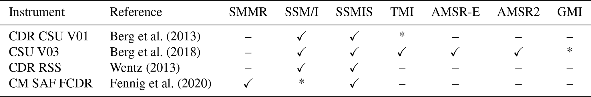
Table 1 lists the major FCDRs from passive microwave imagers available to the community, indicating the inter-calibrated instruments, and the reference instrument. The EUMETSAT Climate Monitoring Satellite Application Facility (CM SAF), Colorado State University (CSU), and Remote Sensing Systems (RSS) all include the SSM/I and Special Sensor Microwave-Imager/Sounder (SSMIS) in their inter-calibrations. CSU uses for the first time GMI in their recent inter-calibration scheme (Berg et al., 2018). They simultaneously employ multiple calibrations methods to reduce the uncertainty in the data record. Their initial work (V01) is improved by adding more satellites and by using GMI as the reference for its description of the diurnal cycle over land. RSS's inter-calibration effort is essentially based on the use of a radiative transfer model over ocean (Wentz, 2013). The CM SAF uses SSM/I F11 as their reference satellite. The inter-calibration is a scene-dependent correction. It is done by correcting the cold end of the observed SMMR–ERA T_b differences to match the SSM∕I–ERA T_b differences but keeping the warm calibration end at the observed hot load target temperature. It is therefore not expected to have an impact on the warm T_b range.

So far, only the CM SAF includes SMMR in their fundamental climate data records (FCDRs). The inter-calibration was developed initially for the monitoring of fluxes over the ice-free ocean (Andersson et al., 2010). To extend the climate record of satellite-derived land surface parameters in time, here we propose to analyze the possibility of inter-calibrating the SMMR instrument over land. The SMMR instrument failed in August 1987, and the first SSM/I (F08) was launched in 1987, with an overlapping time of only a few weeks, and with ∼6 h differences in their overpassing times at the Equator. Here, we suggest to use GMI as a reference instrument, assuming that the environmental conditions have not changed drastically from the SMMR to the GMI era, to allow the comparison of a large set of observations averaged over time. This strategy does not allow a detailed inter-calibration to be performed, but it makes it possible to correct for major biases that so far have hampered the use of SMMR over land for the generation of climate records of geophysical parameters. We will concentrate on the channels that are common to all the microwave imagers used in the FCDR in Table 1, the Ku (around 18 GHz) and Ka (around 36 GHz) channels. These are key observations for the retrieval of several land surface parameters (e.g., surface water extent (Prigent et al., 2007), snow water equivalent (Pulliainen, 2006), or land surface temperature (Jiménez et al., 2017)). We will use the CM SAF FCDR for SMMR data set as the starting point of our developments.

In Sect. 2, the satellite observations used in this study are briefly described, along with their preprocessing for the analysis. The result of the inter-comparison is presented in Sect. 3, along with the proposed inter-calibration procedure and its evaluation. Section 4 concludes this study.

2 Data and method

2.1 The satellite data

Table 2 summarizes the major characteristics of the SMMR and GMI instruments for the Ku and Ka channels. SSM/I on board F08 is also included, as it is the only instrument with an overlap period with SMMR (albeit of only 28 d), and it will be used for evaluation. GMI, with its non-Sun-synchronous orbit, observes the full diurnal cycle, including the SMMR and SSM/I overpassing times.

SMMR was launched in 1978 on the Nimbus-7 satellite and operated until August 1987. It is the first multichannel microwave imager, designed mainly for oceanic applications to estimate the surface wind speed and sea surface temperature (Gloersen and Barath, 1977). Due to power limitation on board, measurements were performed only every other day. The EIA decreases from 50.2 to 49.3^∘ starting in 1986. The initial SMMR record used by the CM SAF is the Level 1B data, not the raw counts that are not available. The SMMR Level 1B data are described by Njoku (1980) and include the antenna pattern and spillover correction, as well as sensor drift correction. The calibration uses the cosmic background temperature as a cold reference (2.7 K), an on-board hot calibration load around 300 K, and climatological means to estimate biases in the calibrations. A linear calibration was performed to reduce instrument bias in the target domain, i.e., for ocean surface parameter estimations. The inter-calibration performed by the CM SAF is based on the double-difference technique between the SSM/I F08 and SMMR brightness temperatures (T_bs), using radiative transfer simulations from reanalysis to account for the changes in frequencies, bandwidths, and EIA. This correction is computed only over cloud-free water surfaces. It is described in detail in Fennig et al. (2020). In this study, we will only use SMMR data showing the best quality (data with sun intrusion, field-of-view, or scan error are removed).

Table 2 The major characteristics of the passive microwave imagers, directly relevant to this study. The instruments include other channels, but they are not used here.

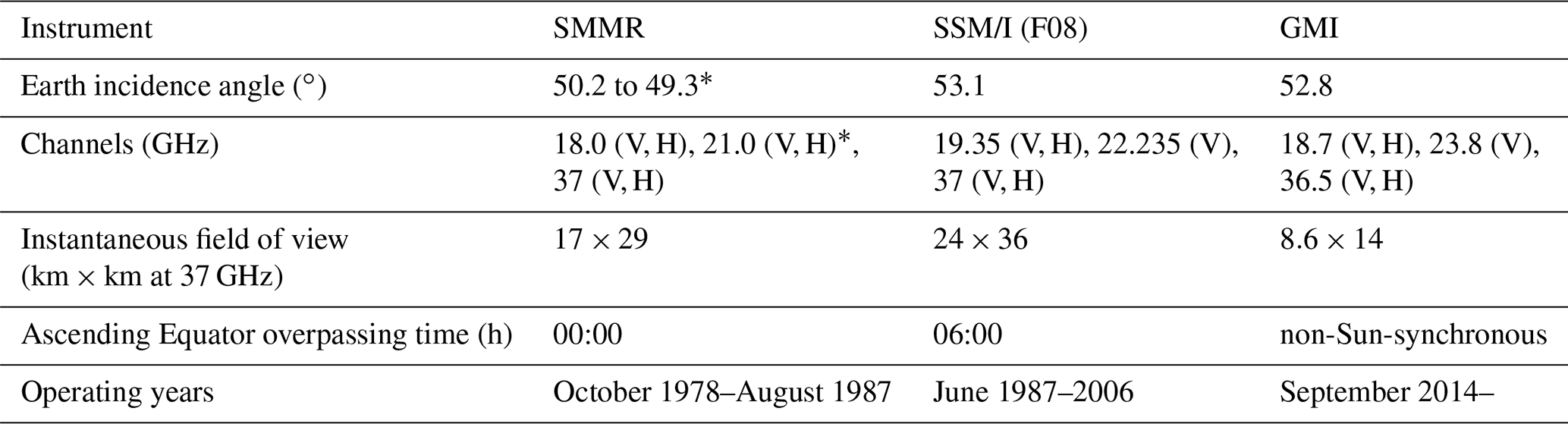
^* Failure of the 21 GHz channel in 1985 and drift from 1986.

GMI is a recent microwave imager launched in 2015. It observes between 10 and 190 GHz to measure precipitation across the globe. It will be used here as a reference standard for calibration. The instrument characteristics are summarized in Table 2, listing only the channels relevant to this study. The satellite has a 65^∘ inclination, allowing non-Sun-synchronous observations of the Earth, from the tropics to the high latitudes. The antenna has an EIA of 52.8^∘ and a swath of ∼900 km. This swath width associated with the inclination means that polar regions are not fully covered. The GMI calibration is described by Wentz and Draper (2016). In addition to the usual hot load, GMI uses noise diodes, improving calibration accuracy. The satellite can also perform flight maneuvers to correct drift and improve calibration. Lean (2017) found low biases for all channels, as compared to ECMWF simulations (lower than 0.8 K). All these technical specificities make GMI an excellent reference for inter-calibration purposes. In this study, the calibrated T_b Level 1C data (Hou et al., 2014) are used.

The first SSM/I was launched in 1987 on board the F08 satellite of the Defense Meteorological Satellites Program (DMSP). In the following years multiple instruments were launched, such as the TMI in 1997 and the SSMIS in 2003. The DMSP polar orbiters cannot correct orbital degradation; as a consequence, the instruments are subject to drifts in the overpassing times, making instrument inter-calibration more challenging. Here, the SSM/I data provided by the CM SAF without the inter-calibration layer will be used to evaluate the consistency of our SMMR land calibration.

2.2 The method

SMMR and GMI do not have any common observing period. Therefore we need to rely on a statistical analysis of SMMR and GMI observations from different years to provide a correction of the SMMR biases over continental surfaces. The fundamental hypothesis here is that the changes in the environmental conditions affecting the microwave signals are limited between the 1980s and 2010s, as compared to the SMMR and the GMI instrument calibration differences.

The SMMR and GMI EIA difference is $\sim \mathrm{3}{}^{\circ }$. Over ocean, this can strongly affect the signal, due to the sensitivity of the ocean emissivity to the incidence angle as well as to the changing atmospheric contribution with angle. Over land, the surface emissivity is usually high for both polarizations, with values of 0.9 and higher for most surface types (Prigent et al., 2006), with very limited changes with EIA (Prigent et al., 2000). With a high land surface emissivity, the atmospheric contribution to the signal is small compared to the surface one and the changes in the atmospheric contribution with angle will not significantly affect the measurement. By the same token, with the land surface emissivities being rather high and showing very smooth variations with frequency (Prigent et al., 2000), the differences in frequencies between the Ku and Ka channels of SMMR and GMI are not expected to significantly affect the signals.

To facilitate the comparison, each data set is projected on the Equal-Area Scalable Earth (EASE)-Grid 2.0 globally between 60^∘ S and 70^∘ N and on the EASE Southern Hemisphere azimuthal grid over the area of Antarctica (Brodzik et al., 2012). A land mask is used to filter out water pixels at 25 km resolution.

GMI data are collected for the months of January, February, July, and August from 2015 to 2017. These 4 months per year include the boreal summer and winter T_b diurnal cycles, and with data sampled from the whole Earth most of the possible surface conditions are represented in the analyzed data set. As GMI has a higher spatial resolution than the target grid, all observations falling within a grid cell of ∼12 km radius are averaged to derive one value per grid cell. Regarding the temporal dimension, the values are averaged with a 15 min window for each grid cell to suppress small-scale variability in the signal. If no observation in a given grid cell is available in a particular 15 min interval, a linear interpolation with the closest existing measurements is performed. Finally, to get a smooth diurnal cycle, a moving average is applied over each grid cell with a 75 min window (two data points before and after the target one).

For SMMR, T_bs are collected from 1981, 1982, and 1987 for the same months as GMI. The observations are available twice a day (for the ascending and descending overpasses). Given the comparable resolutions of SMMR observations and the target grid, a nearest-neighbor technique is used to project the T_bs onto the EASE grid. Using several years of data for each instrument can alleviate possible effects of strong inter-annual variability in the signals (related to El Niño or La Niña events for instance).

The resulting data sets contain almost 2 million data points spanning all the continents and two contrasted seasons (summer and winter).

3 Results

3.1 SMMR and GMI comparisons at the regional scale

At regional scales, a set of different areas have been selected to represent large variability in environmental conditions. The averaged T_bs diurnal cycle derived from GMI is calculated for sample areas covering 25 grid cells, over 2 months, over 3 years (2015–2017). Over these areas, covering roughly a $\mathrm{1}{}^{\circ }\times \mathrm{1}{}^{\circ }$ surface, the averaged SMMR T_bs for the ascending and descending orbits are also calculated, over the same months, for 1981, 1982 and 1987.

Figure 1 presents the results for areas in the North Hemisphere, during winter (January and February), at 18 and 37 GHz, for both orthogonal polarizations. It includes cold mountainous regions, arid deserts with high T_bs during the day and a large amplitude of the diurnal cycle, and warm rainforest with a limited variation in T_bs. Forested regions show a low diurnal cycle amplitude of the T_bs (<10 K), with almost no difference between V and H polarizations due to the emission and scattering effect of the dense vegetation. Arid regions (cold or warm) have large diurnal variations in T_bs, directly related to the diurnal cycle of the land surface temperature. The polarization difference is significant, due to an almost specular behavior of these rather flat surfaces. With increasing vegetation cover (sparsely vegetated or grassland) an intermediate behavior is observed. The variability associated to each GMI average is computed and also displayed (the grey shades around the diurnal cycle indicate 1 standard deviation). The number of individual pixels used in the diurnal cycle calculation is also indicated (blue shades). The low variability of the signals over the Amazon confirms the high stability of the T_bs in this region, which is regularly used as a warm radiometric reference (e.g., Brown and Ruf, 2005). The SMMR values have been calculated for the initial Level 1B data as well as for the CM SAF inter-calibrated results, but only the Level 1B data are displayed in Fig. 1. Note that the CM SAF inter-calibration is neither designed nor validated for observations over land.

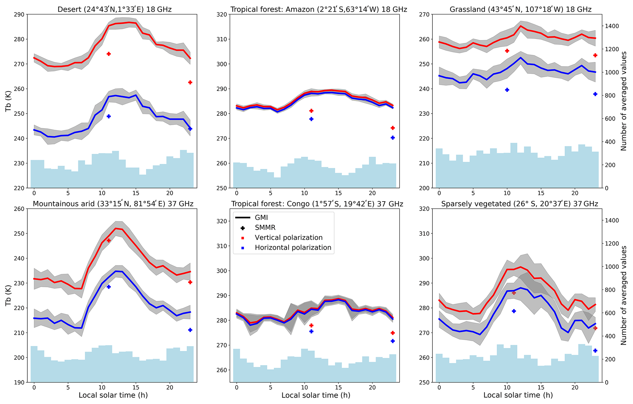
Figure 1 Diurnal cycles from GMI compared to SMMR values at different frequencies and locations averaged for the months of January and February (horizontal polarization in blue and vertical in red). Measurements are averaged over 25 grid cells and by hour, with the standard deviation of each average temperature in the diurnal cycle and the associated number of measurements displayed below.

The SMMR day and night values follow the same diurnal pattern as GMI, but with a systematic underestimation of the T_bs, regardless of the frequency and polarization. These differences are usually significantly larger than what is expected from the GMI signal variability, indicated by the standard deviation around the average. The difference between SMMR and GMI appears to be almost the same for both polarizations. The difference seems to decrease for the coldest locations. The variability is higher at midlatitudes, where year-on-year variations are possible and meteorological events can impact the measurements. The differences cannot be explained solely by the instruments' different characteristics (EIA or frequencies) or by environmental changes between the periods covered by the two instruments (the 1980s for SMMR and the 2010s for GMI). Different sources could cause such errors, for instance an erroneous warm calibration load temperature or an error in the correction of antenna pattern that misses the Earth.

The inter-calibration layer from CM SAF for SMMR does not seem to improve the results. Over land the mean correction added by the calibration is below 0.5 K for the 18 GHz vertical and horizontal polarization and 37 GHz horizontal channel. The correction for the 37 GHz vertically polarized channel is on average around 2 K. The inter-calibration has been designed mainly for ocean observations with low T_bs and not for land applications, so it does not adequately correct for calibration issues over land (not shown in the figure). Other locations and seasons were analyzed, with similar conclusions (not shown here).

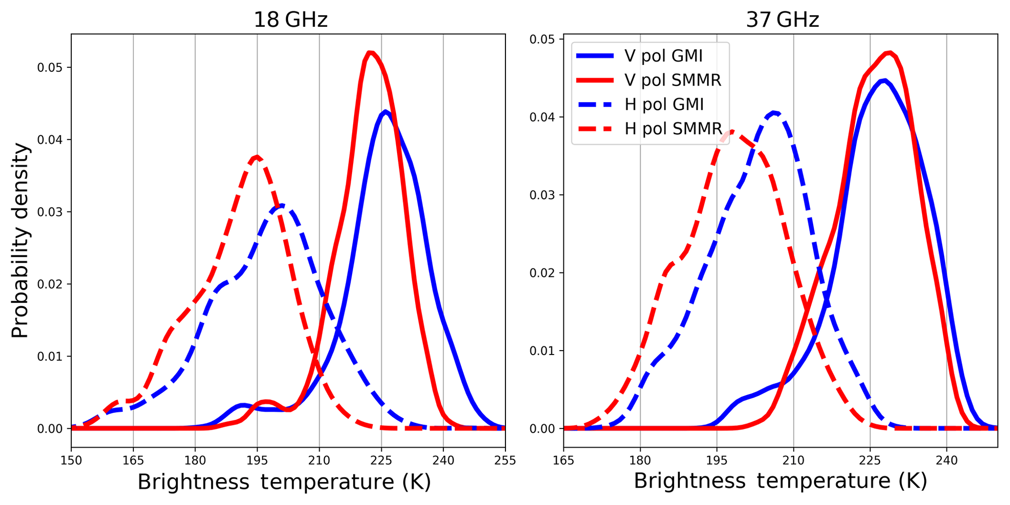
Figure 2 Probability density functions of July/August brightness temperatures over Antarctica for GMI in 2015 and SMMR in 1987.

The observations over the Antarctic ice sheet are also explored, to extend our investigation to lower T_bs. Because of the GMI coverage, the comparison is limited to the edge of Antarctica. Care is exercised to avoid contamination by the ocean and sea ice. Southern Hemisphere winter months are selected (July and August). During this long night, there is no diurnal cycle and the T_bs distribution for the two satellites are directly compared (Fig. 2). The delta between SMMR Level 1B and GMI T_bs distribution is between 5 and 10 K for all channels except the 37 GHz vertical polarization, which shows a lower difference.

Here as well, the significant differences in the SMMR Level 1B and GMI T_bs cannot be attributed only to changes in environmental conditions, even over ∼30 years. Jezek et al. (1993) compared SMMR and SSM/I over the Antarctic ice sheet during their overlap period and also found significant differences in both Ku and Ka bands. They discussed the impact of the change in EIA and frequency between the instruments but concluded that it cannot explain the large observed differences. Only calibration issues can explain the observed differences, with the SMMR T_bs colder than the GMI ones.

3.2 Derivation of a SMMR correction over continental surfaces

In order to assess the possibility to correct for the SMMR calibration issue, SMMR and GMI observations are compared at the global scale. The SMMR observations (both ascending and descending orbits) are compared to the corresponding GMI values for the same times in the day, for January and February and for July and August, over 3 years for the two instruments (1981, 1982, and 1987 were used for SMMR and 2015 to 2017 for GMI, as before). Points for which the difference between the GMI and SMMR values is outside 3 standard deviations from the mean difference are suppressed. We checked that these points were essentially located over coastal regions: GMI has a better spatial resolution than SMMR, and over the coasts the SMMR observations will likely include more contributions from the surrounding ocean. Figure 3 displays the distribution of the GMI against the SMMR T_bs, at 18 and 37 GHz, for both polarizations. The underestimation of the SMMR T_bs compared to the GMI ones clearly increases with T_bs. Here we suggest a simple linear correction to inter-calibrate the SMMR observations toward the GMI ones. A more sophisticated correction would not be justified. First, we are aware that this is a first-order inter-calibration, as the comparison involves different years. Second, it would be more complex to implement especially in processing chains. Lastly, it would likely overfit some part of the signal rather than correcting the T_bs.

A simple correction is proposed for all channels with the form ${\widehat{T}}_{\text{SMMR}}=a\times T_{\text{SMMR}}+b$. The coefficients slope a and the intercept b are estimated through the minimization of the sum of squared difference: ${\sum }_{i=\mathrm{1}}^N(T_{\text{GMI}}-a\times T_{\text{SMMR}}-b{)}^{\mathrm{2}}$, derived from the assumption that ${\widehat{T}}_{\text{SMMR}}=T_{\text{GMI}}$, with N being the number of data points used for the regression coefficient estimation. The data collection covers the full T_b range observable over continental surfaces, including some polar regions.

Figure 3 Linear regression on SMMR values against GMI after filtering points. In addition the correction derived by Dai and Che (2009) (and corrected for the SSM/I F08-to-GMI calibration) is displayed.

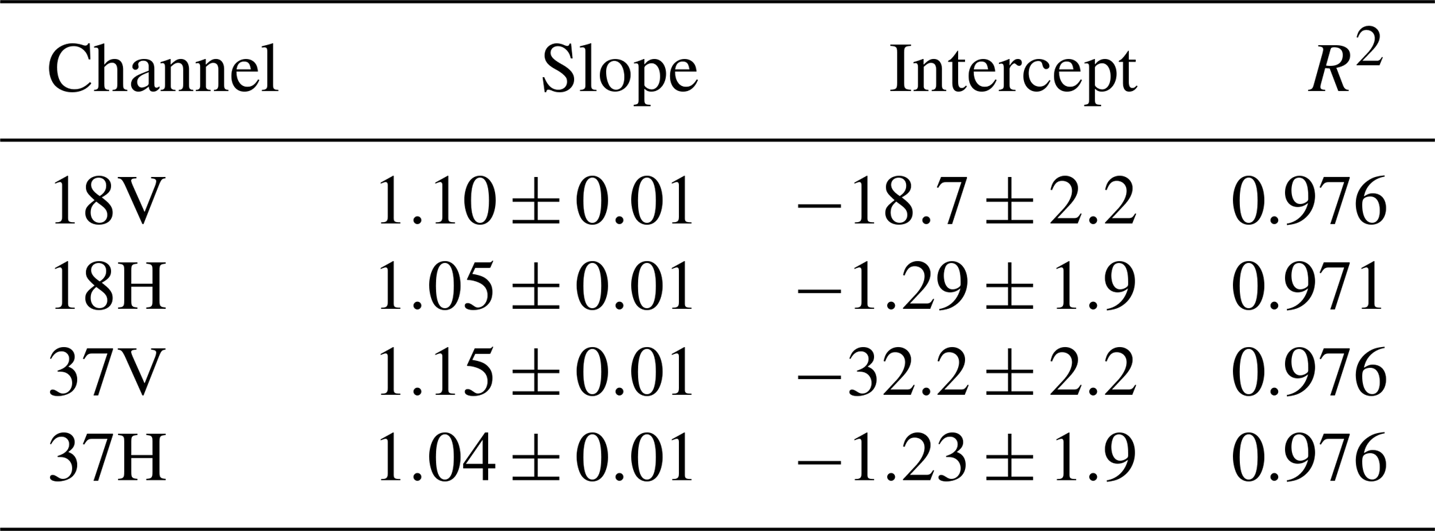
The distribution of the data points from the cold and warm ends is uneven, with fewer points for lower T_bs. To alleviate this issue, we randomly sample the points from both the cold and warm ends to simulate an even distribution over the full T_b range. Different samplings were tested to confirm the stability of the estimated coefficients. The resulting regression lines are added to Fig. 3. The mean squared errors of the linear regression are indicated with grey shades. It appears clearly that the uncertainty in the areas with fewer data (between the Antarctica temperatures and the land data points) or near the edge of the range of values are the ones with the highest errors. The coefficients of the linear regressions are provided in Table 3. The uncertainties on the regression coefficients are computed with a t test for a 99 % confidence level.

Table 3 Estimated linear correction coefficients, for the inter-calibration of the SMMR observations at 18 and 37 GHz, vertical and horizontal polarizations, with respect to GMI observations over the continents. The uncertainties are also added (computed with a t test at the 99 % confidence level).

3.3 Evaluation

The suggested corrections are applied to SMMR values, and the results can be compared to other imager observations. With the inter-calibration being derived from GMI, a good agreement is expected with that sensor. The first check consists in comparing the calibrated SMMR observations to the SSM/I observations, for their overlapping period. The GMI-derived diurnal cycle of T_bs is used as a bridge between the SMMR and SSM/I observations that have different overpassing times. Figure 4 presents the comparisons of SMMR and SSM/I F08, for different locations, averaged over their common period in July and August 1987, along with the GMI-derived diurnal cycle of the T_bs (estimated over 3 different years). It shows that SSM/I T_bs, used without any inter-calibration, are in good agreement with the T_b diurnal cycle estimated from GMI. Contrarily to the SMMR observations before inter-calibration, no obvious large bias is observed between SSM/I and GMI, even for the very warm scenes, at 18 and 37 GHz for both polarizations. The average difference between SSM/I F08 and GMI (without any inter-calibration scheme applied) is around 2.5 K for the 18 GHz channels and around 0.5 K for the 37 GHz channels. A bias is expected between measurements that have not been inter-calibrated, but it is lower than the one detected for SMMR and confirms our assumptions regarding the emissivity behavior over continental surfaces as well as the small variation in environmental conditions in the 30-year gap between the 1980s and the 2010s.

Figure 4 Diurnal cycle of GMI in July/August compared to values measured by SMMR with and without the proposed correction, and SSM/I values for the months of July/August 1987 over various locations and at different frequencies.

The agreement between the SMMR inter-calibrated values and GMI is clearly improved, as compared to the previous SMMR Level 1B results. These results show that the SSM/I F08 and the newly inter-calibrated SMMR are consistent, at least within the uncertainty provided with this inter-calibration. More cases have been tested, with similar results (not shown here).

In addition to the evaluation with other sensors, the results of our inter-calibration are compared with an alternative method developed for SMMR. Dai and Che (2009) built their inter-calibration scheme upon observations in desert and polar areas. The SSM/I F08 instrument is adopted as the reference, and a model is developed to account for the diurnal changes in temperatures. The resulting linear regressions are added in Fig. 3 (green dotted lines). The two inter-calibration methods are based on very different principles. Nevertheless, they agree well for all channels, with similar slopes and slightly different intercepts. This adds confidence to our methodology.

4 Conclusions

Several FCDRs from passive microwave imagers have been produced, from pioneer instruments such as SMMR to the AMSR series. So far, the efforts have essentially focused on oceanic regions, where radiative transfer simulations fed by reanalysis can serve as a reference to bridge the differences between the instruments, in terms of frequency, EIA, and overpassing time. Over continental surfaces, inter-calibration of passive microwave imagers is challenging, especially for Sun-synchronous polar-orbiting satellites with different overpassing times at the Equator. Here we derived a method to extend the FCDR collection to SMMR over land at 18 and 37 GHz, using the non-Sun-synchronous GMI instrument as a reference, despite the lack of a common observing period. GMI observations are used to reconstruct the diurnal cycles of T_bs that should be observed with SMMR, with the assumption that the environmental conditions have not changed drastically over the last 30 years and that the differences in frequencies and EIA between the two instruments can be neglected over land. With these hypotheses, the objective is to correct for the large differences between the sensors. Before inter-calibration, the comparison of the SMMR and GMI observations shows a significant underestimation of the T_bs with SMMR, and this underestimation tends to increase with increasing T_bs. A linear regression is suggested for the 18 and 37 GHz channels, vertical and horizontal polarizations, to calibrate the SMMR observations toward the GMI estimates. The SMMR correction is evaluated with respect to the SSM/I F08 observations over their overlapping period in orbit, in July and August 1987. The GMI-derived diurnal cycle of T_bs acts as a bridge between the two instruments that have different overpassing times. A good agreement is reached between all sensor measurements. This inter-calibration of the SMMR instrument over land will make it possible to extend the passive microwave estimations of land surface variables over 9 more years backward, from 1978 to 1987. However, given the use of the more recent GMI instrument as a calibration reference, and the uncertainty regarding the calibration error sources as well as the validity of the environmental stability hypothesis, any comparison between the different epochs should be conducted with extreme care. The use of this correction to derive climate series should be thoroughly assessed before using it. This will be practically tested in the near future for the estimates of, for instance, surface water extent and land surface temperatures from microwave observations, two variables that rely on the 18 and 37 GHz observations for their retrieval, under clear and cloudy-sky conditions.