the Creative Commons Attribution 4.0 License.
the Creative Commons Attribution 4.0 License.
 | 15 Oct 2020
Satellite validation strategy assessments based on the AROMAT campaigns
Alexis Merlaud
Livio Belegante
Daniel-Eduard Constantin
Mirjam Den Hoed
Andreas Carlos Meier
Marc Allaart
Magdalena Ardelean
Maxim Arseni
Tim Bösch
Hugues Brenot
Andreea Calcan
Emmanuel Dekemper
Sebastian Donner
Steffen Dörner
Mariana Carmelia Balanica Dragomir
Lucian Georgescu
Anca Nemuc
Doina Nicolae
Gaia Pinardi
Andreas Richter
Adrian Rosu
Thomas Ruhtz
Anja Schönhardt
Dirk Schuettemeyer
Reza Shaiganfar
Kerstin Stebel
Frederik Tack
Sorin Nicolae Vâjâiac
Jeni Vasilescu
Jurgen Vanhamel
Thomas Wagner
Michel Van Roozendael
The Airborne ROmanian Measurements of Aerosols and Trace gases (AROMAT) campaigns took place in Romania in September 2014 and August 2015. They focused on two sites: the Bucharest urban area and large power plants in the Jiu Valley. The main objectives of the campaigns were to test recently developed airborne observation systems dedicated to air quality studies and to verify their applicability for the validation of space-borne atmospheric missions such as the TROPOspheric Monitoring Instrument (TROPOMI)/Sentinel-5 Precursor (S5P). We present the AROMAT campaigns from the perspective of findings related to the validation of tropospheric NO2, SO2, and H2CO. We also quantify the emissions of NOx and SO2 at both measurement sites.
We show that tropospheric NO2 vertical column density (VCD) measurements using airborne mapping instruments are well suited for satellite validation in principle. The signal-to-noise ratio of the airborne NO2 measurements is an order of magnitude higher than its space-borne counterpart when the airborne measurements are averaged at the TROPOMI pixel scale. However, we show that the temporal variation of the NO2 VCDs during a flight might be a significant source of comparison error. Considering the random error of the TROPOMI tropospheric NO2 VCD (σ), the dynamic range of the NO2 VCDs field extends from detection limit up to 37 σ (2.6×10¹⁶ molec. cm−2) and 29 σ (2×10¹⁶ molec. cm−2) for Bucharest and the Jiu Valley, respectively. For both areas, we simulate validation exercises applied to the TROPOMI tropospheric NO2 product. These simulations indicate that a comparison error budget closely matching the TROPOMI optimal target accuracy of 25 % can be obtained by adding NO2 and aerosol profile information to the airborne mapping observations, which constrains the investigated accuracy to within 28 %. In addition to NO2, our study also addresses the measurements of SO2 emissions from power plants in the Jiu Valley and an urban hotspot of H2CO in the centre of Bucharest. For these two species, we conclude that the best validation strategy would consist of deploying ground-based measurement systems at well-identified locations.
- Article
(17311 KB) - Full-text XML
-
Supplement
(1906 KB) - BibTeX
- EndNote


Since the launch of the Global Ozone Monitoring Experiment (GOME, Burrows et al., 1999) in 1995, spaceborne observations of reactive gases in the UV–visible range have tremendously improved our understanding of tropospheric chemistry. GOME mapped the large urban sources of NO2 in North America and Europe, the SO2 emissions from volcanoes and coal-fired power plants (Eisinger and Burrows, 1998), and the global distribution of H2CO, with its maxima above East Asia and tropical forests (De Smedt et al., 2008). Subsequent air quality satellite missions expanded on the observation capabilities of GOME. Table 1 lists the past, present, and near-future nadir-looking satellite instruments dedicated to ozone and air quality monitoring with their sampling characteristics in space and time. The pixel size at nadir has shrunk from 320×40 km2 (GOME) to 3.5×5.5 km2 (TROPOMI, Veefkind et al., 2012, the original TROPOMI resolution of 7×5.5 km2 was increased on 6 August 2019, MPC, 2019). This high horizontal resolution enables us, for instance, to disentangle contradictory trends in ship and continental emissions of NO2 in Europe (Boersma et al., 2015) or to distinguish the different NO2 sources in oil sand mines in Canada (Griffin et al., 2019). The satellite-derived air quality products are now reliable enough to improve the bottom-up emission inventories (e.g. Kim et al., 2009; Fioletov et al., 2017; Bauwens et al., 2016) and to be used in operational services, e.g. to assist air traffic control with the near-real time detection of volcanic eruptions (Brenot et al., 2014). The bottom lines of Table 1 present the near-future perspective for space-borne observations of the troposphere: a constellation of geostationary satellites will provide hourly observations of the troposphere above east Asia (GEMS, (Kim, 2012)), North America (TEMPO, Chance et al., 2013), and Europe (Sentinel-4, Ingmann et al., 2012). These new developments will open up new perspectives for atmospheric research and air quality policies (Judd et al., 2018).
Table 1Past and near-future space missions focused on air quality: coverage, pixel size, and temporal sampling.

Validation is a key aspect of any space-borne Earth observation mission. This aspect becomes even more important as the science matures and leads to more operational and quantitative applications. Validation involves a statistical analysis of the differences between measurements to be validated and reference measurements, which are independent data with known uncertainties (von Clarmann, 2006; Richter et al., 2014). The aim of validation is to verify that the satellite data products meet their requirements in terms of accuracy and precision. Table 2 presents such requirements for the TROPOMI-derived tropospheric vertical column densities (VCDs) of NO2, SO2, and H2CO (ESA, 2014). Richter et al. (2014) discussed the challenges associated with the validation of tropospheric reactive gases. These challenges arise from the large variability in space and time of short-lived reactive gases, the dependency of the satellite products on different geophysical parameters (surface albedo, profile of trace gases and aerosols), the differences in vertical sensitivity between satellite and reference (ground-based or airborne) measurements, and the small signals. An ideal validation study would involve a reference dataset of VCDs, whose well-characterised uncertainties would be small compared to those required for the investigated products. This reference dataset would cover a large amount of satellite pixels with adequate spatial and temporal representativeness at different seasons, places, and pollution levels. Alongside the VCDs, the ideal validation exercise would also quantify the geophysical parameters that impact the retrieval of the investigated satellite products. In the real world, however, Richter et al. (2014) points out that “the typical validation measurement falls short in one or even many of these aspects”.
Table 2Data quality targets for the S5P TROPOMI data products relevant in the AROMAT context (extracted from ESA, 2014).

The first validations of the tropospheric NO2 and H2CO VCD products of GOME involved in situ samplings from aircraft (Heland et al., 2002; Martin et al., 2004). Such measurements may cover large fractions of satellite pixels, but they miss the lower part of the boundary layer, where the trace gas concentrations often peak. Schaub et al. (2006) and Boersma et al. (2011) summarise other early validation studies for the tropospheric NO2 VCDs retrieved from GOME, SCIAMACHY, and OMI. Several of these studies make use of the NO2 surface concentration datasets from air quality monitoring networks. Compared to campaign-based data acquisition, operational in situ networks provide long-term measurements, but their comparison with satellite products relies upon assumptions on the NO2 profile. Other validation studies use remote sensing from the ground and aircraft, in particular based on the Differential Optical Absorption Spectroscopy (DOAS) technique (Platt and Stutz, 2008), which is also the basis for the retrieval algorithms of the satellite-derived products. In comparison with in situ measurements, DOAS has the benefit of being directly sensitive to the column density of a trace gas, i.e. the same geophysical quantity as the one retrieved from space. Heue et al. (2005) conducted the first comparison between a satellite-derived product (SCIAMACHY tropospheric NO2) and airborne DOAS data. Many validation studies also use ground-based DOAS measurements, in particular since the development of the Multi-AXis DOAS (MAX-DOAS) technique (Hönninger et al., 2004). MAX-DOAS measurements are valuable for validation due to their ability to measure integrated columns at spatial scales comparable to the satellite ground pixel size. Moreover, they broaden the scope of validation activities since they also provide limited profile information on both trace gases and aerosols (Irie et al., 2008; Brinksma et al., 2008; Ma et al., 2013; Kanaya et al., 2014; Wang et al., 2017; Drosoglou et al., 2018). The limitations of using the MAX-DOAS technique for validation arise from their still imperfect spatial representativeness compared to typical satellite footprints and, to some extent, from their limited sensitivity in the free troposphere. Spatial representativeness has often been invoked to explain the apparent low bias of the OMI tropospheric NO2 VCDs in urban conditions (Boersma et al., 2018).
The unprecedented horizontal resolution enabled by the last generation of air quality space-based instruments motivated preparatory field studies around polluted areas in North America (DISCOVER-AQ, https://discover-aq.larc.nasa.gov, last access: 8 October 2020), Europe (AROMAT and AROMAPEX, Tack et al., 2019), and Korea (KORUS-AQ, https://www-air.larc.nasa.gov/missions/korus-aq/, last access: 8 October 2020). These campaign activities quantified key pollutants (NO2, SO2, O3, H2CO, and aerosols) and assessed practical observation capabilities of future satellite instruments while preparing for their validation. They combined ground-based and airborne measurements. DISCOVER-AQ involved the deployment of the Geostationary Trace gas and Aerosol Sensor Optimization instrument (GEOTASO, Leitch et al., 2014; Nowlan et al., 2016) and of the Geostationary Coastal and Air Pollution Events (GEO-CAPE) Airborne Simulator (GCAS, Kowalewski and Janz, 2014; Nowlan et al., 2018). In Europe, the two AROMAT campaigns, which took place in Romania in September 2014 and August 2015, demonstrated a suite of new instruments, such as the Airborne imaging DOAS instrument for Measurements of Atmospheric Pollution (AirMAP, Schönhardt et al., 2015; Meier et al., 2017), the NO2 sonde (Sluis et al., 2010), and the Small Whiskbroom Imager for atmospheric compositioN monitorinG (SWING, Merlaud et al., 2018). Different airborne imagers were intercompared and further characterised during the AROMAPEX campaign in April 2016 (Tack et al., 2019).
Two aforementioned publications focused on the AirMAP and SWING operations during the 2014 AROMAT campaign (Meier et al., 2017; Merlaud et al., 2018). In this work, we present the overall instrumental deployment during the two campaigns and analyse the relevance of these measurements for the validation of several air quality satellite products: tropospheric NO2, SO2, and H2CO VCDs. The datasets collected during AROMAT fulfil several requirements of the ideal validation study, as described above. We further investigate the strengths and limitations of the acquired data sets.
The paper is structured as follows: Sect. 2 describes the two target areas and the deployment strategy. Section 3 characterises the investigated trace gases fields in the sampled areas. Section 4 presents a critical analysis of the strengths and limitations of the campaign results while elaborating on recommendations for future validation campaigns in Romania. Eventually, we use the AROMAT measurements to derive NOx and SO2 fluxes from the two sites. The Supplement presents technical details on the instruments operated during the campaigns and presents additional information and measurements.
This section presents the two target areas of the AROMAT campaigns, Bucharest and the Jiu Valley. It also lists available studies on air quality at these two sites and logistical aspects of relevance.
Figure 1 presents a map of the tropospheric NO2 vertical column densities (VCDs) above Romania, derived from OMI measurements (Levelt et al., 2006) and averaged between 2012 and 2016. The map also indicates the position of the eight largest cities in the country. Compared to highly polluted areas in western Europe, such as northern Belgium or the Netherlands, Romania appears relatively clean at the spatial resolution of the satellite data. There are, however, two major NO2 sources that are clearly visible from space, which appear to be of similar magnitude with NO2 columns around 2.5×10¹⁵ molec. cm−2: the Bucharest area and the Jiu Valley, northwest of Craiova. For the latter, the NO2 enhancement is due to a series of large coal-fired thermal power plants.
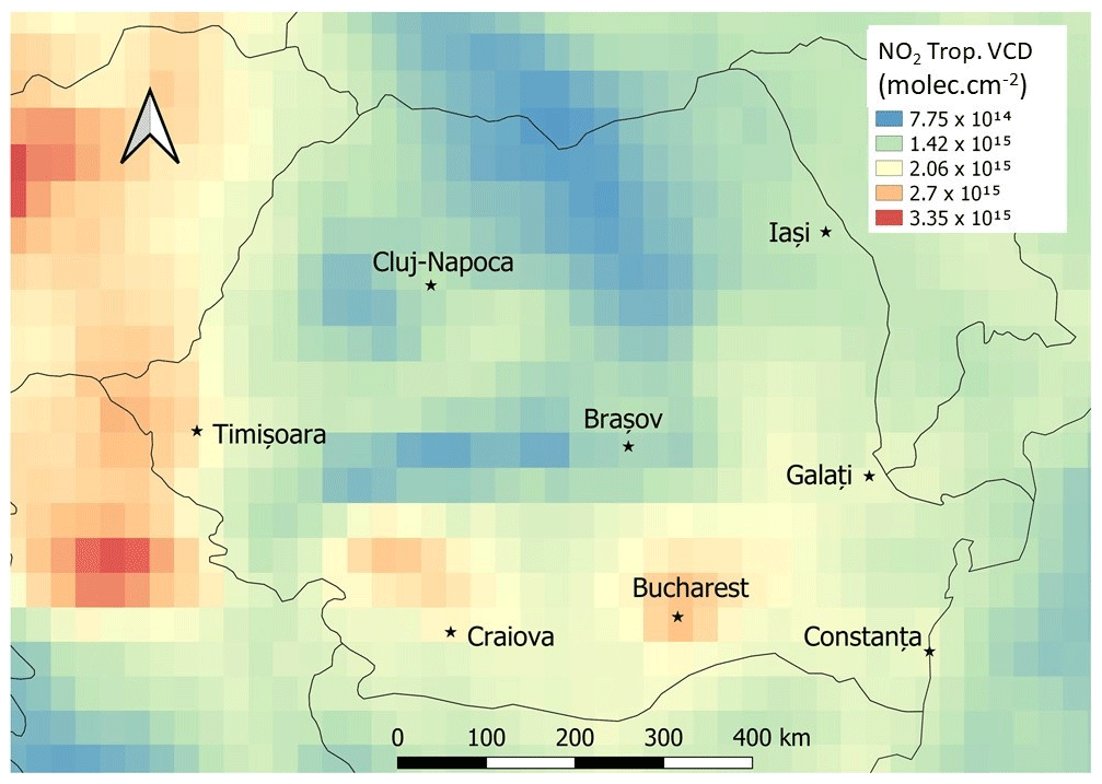
Figure 1The tropospheric NO2 VCD field seen from space with the OMI/AURA instrument above Romania (OMNO2d product, averaged for 2012–2016 with Giovanni, NASA GES DISC). The black stars pinpoint the largest cities in Romania.
2.1 Bucharest
Bucharest (44.4∘ N, 26.1∘ E) is the capital and largest city (1.9 million inhabitants according to the 2011 census) of Romania. Within its administrative borders, the city covers an area of 228 km2. Adding the surrounding Ilfov County, the total Bucharest metropolitan area numbers 2.3 million inhabitants across 1583 km2. The built-up areas are mainly located within a ring road whose diameter is around 20 km.
Iorga et al. (2015) described the Greater Bucharest Area in detail in the context of an extensive study of the air quality in the city between 2005 and 2010. Bucharest is located in a low-altitude plain, with a maximum altitude of 92 m a.s.l. The geographic configuration of the Carpathian Mountains explains the dominant northeasterly winds.
The NO2 VCDs seen from space above Bucharest appear lower than over western European sites at the resolution of OMI (see Fig. S1 in the Supplement). However, this is partly due to the dilution effect for this relatively small and isolated source. Local studies based on the eight air quality stations inside the city point out that Bucharest is amongst the most polluted cities in Europe in regard to local PM and NOx levels (Alpopi and Colesca, 2010; Iorga et al., 2015). The city centre is the most heavily polluted, with concentrations of pollutants well above the European thresholds. For instance, the annual mean concentration of NO2 at the traffic stations was about 57 µg m−3 in 2017 (EEA, 2019), while the EU limit is 40 µg m−3. Stefan et al. (2013) have shown the importance of local conditions and anthropogenic factors in air quality analysis in areas close to Bucharest during 2 weeks of measurements in 2012. Iorga et al. (2015) and Grigoraş et al. (2016) showed that the main NOx contributions came from traffic and production of electricity spread over about 10 medium-sized thermal power plants within the city.
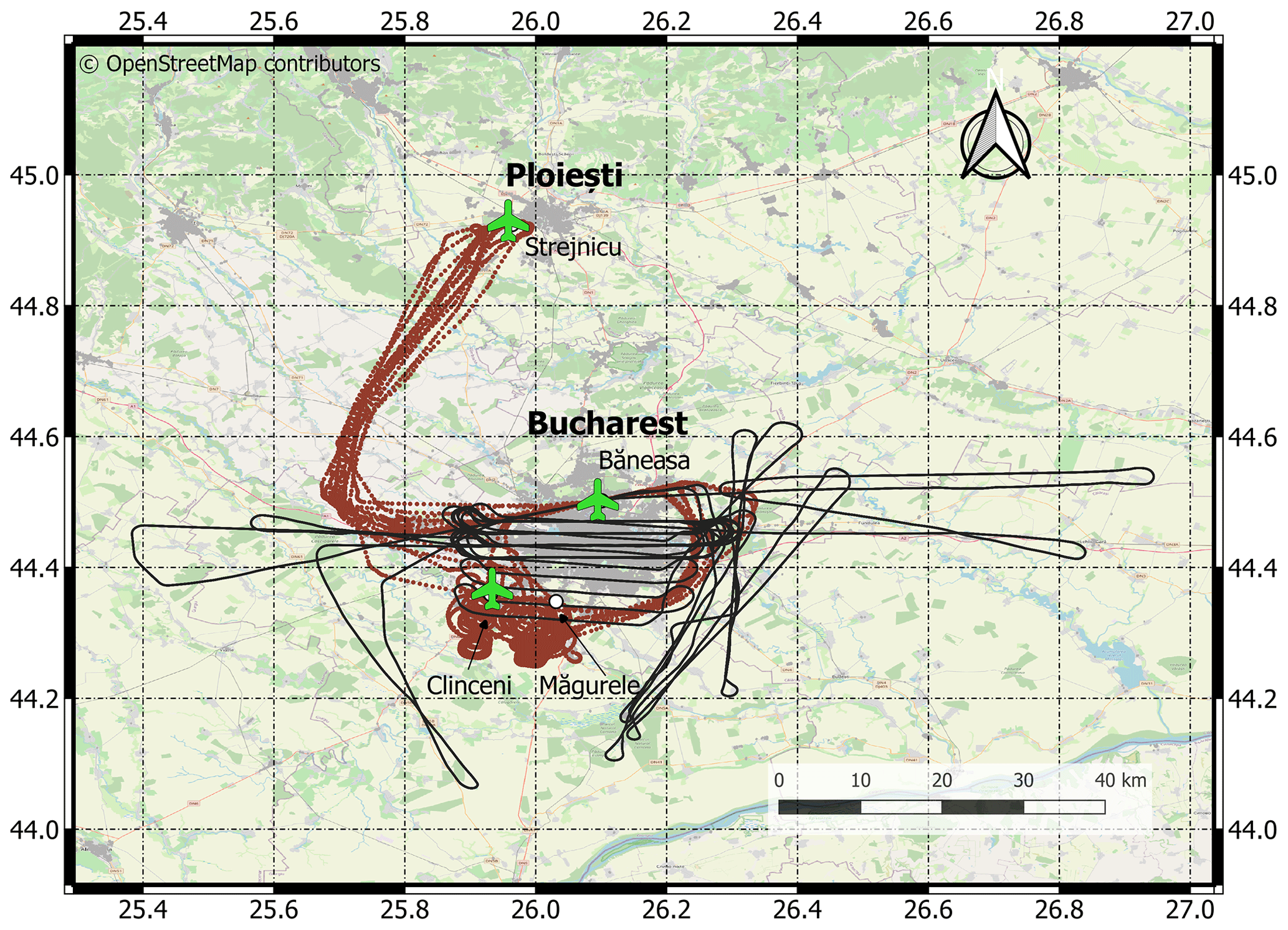
Figure 2The Bucharest area, with important locations for the AROMAT campaigns: the INOE atmospheric observatory in Măgurele, the Băneasa airport, and the Clinceni airfield. Built-up areas appear in grey. The red and black lines, respectively, show the BN-2 and Cessna flight tracks during AROMAT-2.
Figure 2 shows the Bucharest metropolitan area and the flight tracks of the two scientific aircraft used during AROMAT-2 (the FUB Cessna-207 and the INCAS BN-2). Note that the BN-2 tracks are actually a good indication of the Bucharest ring road. We were not allowed to cross the ring road with the BN-2, except to the north of the city. Figure 2 also pinpoints important locations for the AROMAT campaigns. The FUB Cessna took off and landed at the Băneasa international airport, located 8 km north of Bucharest city centre (44.502∘ N, 26.101∘ E). The INCAS BN-2 also used Băneasa airport during AROMAT-2, but this plane was mainly based at the Strejnicu airfield (44.924∘ N, 25.964∘ E), which lies 60 km north of Bucharest, near Ploieşti. The unmanned aerial vehicle (UAV) operations in Bucharest during AROMAT-1 were performed at Clinceni airfield (44.359∘ N, 25.931 ∘ E). The latter is located in the southwest of the city, 7 km west of the INOE observatory in Măgurele (44.348∘ N, 26.031∘ E).
2.2 The Jiu Valley between Târgu Jiu and Craiova
The second NO2 plume in Fig. 1 lies around 250 km west of Bucharest. It corresponds to a series of four thermal power plants located along the Jiu river between the cities of Târgu Jiu (82 000 inhabitants; 45.03∘ N, 23.27∘ E) and Craiova (269 000 inhabitants; 44.31∘ N, 23.8∘ E). These plants were built in this area due to the presence of lignite (brown coal), which is burned to produce electricity.
The altitude of the valley ranges from 268 m a.s.l. in Târgu Jiu to 90 m in Craiova. The valley is surrounded by moderately elevated hills (400 m a.s.l.). Due to the orography, the prevailing wind direction is from southwest to southeast.
Alongside NO2, the SO2 emissions from these plants are also visible from space, as first reported by Eisinger and Burrows (1998) using GOME data. Since 2011, the OMI-derived trends above the area indicate that the emissions of SO2 have been decreasing, while those of NO2 are stable (Krotkov et al., 2016). This is related to the installation of flue gas desulfurisation (FGD) systems, which was part of environmental regulations imposed on Romania following its entry into the European Union in 2007.
Figure 3 presents a map of the Jiu Valley area with the four power plants. The map also shows the tracks of the two airborne platforms (the FUB Cessna and an ultralight aircraft operated by UGAL) operated in this area during AROMAT-2. Table S1 in the Supplement presents the geographical positions, nominal capacities, and smokestack heights of the four power plants. From north to south, the plants are named according to their locations: Rovinari, Turceni, Işalniţa and Craiova II.
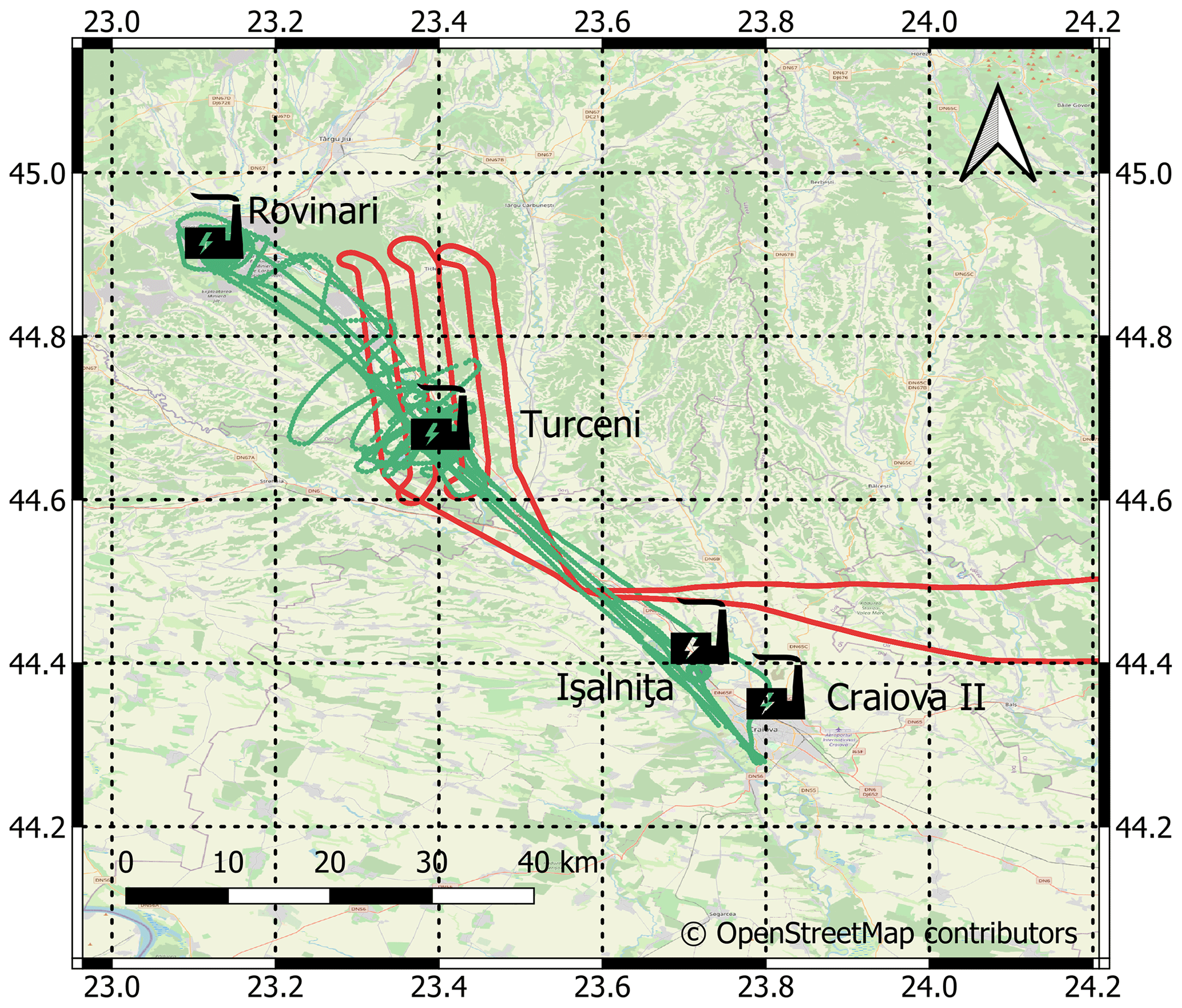
Figure 3The Jiu Valley and its four power plants between Târgu Jiu and Craiova. The scientific crew was based in Turceni during the AROMAT campaigns. The green and red lines, respectively, show the ultralight and Cessna flight tracks during AROMAT-2.
During the AROMAT campaigns, we focused on the emissions of the Turceni power plant (44.67∘ N, 23.41∘ E) in particular. With a nominal capacity of 1650 MW, it is the largest electricity producer in Romania. The Turceni power plant is located in a rural area, 2 km east-southeast of the village of Turceni. The plant emits aerosols, NOx, and SO2 from the 280 m high smokestacks.
Scientific studies on air quality inside the Jiu Valley are sparse. Previous measurements performed by INOE during a campaign in Rovinari in 2010 indicated elevated volume mixing ratios of NO2 (up to 30 ppb) and SO2 (up to 213 ppb) (Nisulescu et al., 2011; Marmureanu et al., 2013). The maximum ground concentrations occurred in the morning, before the planetary boundary layer development. Mobile DOAS observations performed in 2013 revealed columns of NO2 up to 1×10¹⁷ molec. cm−2 (Constantin et al., 2015).
2.3 Groups, instruments, and platforms
The AROMAT consortium consisted of research teams from Belgium (BIRA-IASB), Germany (IUP-Bremen, FUB, MPIC), the Netherlands (KNMI), Romania (University “Dunarea de Jos” of Galaţi, hereafter UGAL; National Institute of R&D for Optoelectronics, hereafter INOE; and National Institute for Aerospace Research “Elie Carafoli”, hereafter INCAS), and Norway (NILU). The AROMAT consortium had the common focus of measuring the tropospheric composition using various techniques.
Figure 4 illustrates the typical instrumental deployment during the campaigns. The set-up combined airborne and ground-based measurements to sample the 3D chemical state of the lower troposphere above polluted areas. The Supplement presents the main atmospheric instruments operated during the two campaigns, classified into airborne, ground-based, remote sensing, and in situ sensors. The primary target species during AROMAT-1 were NO2 and aerosols, while the observation capacities expanded in AROMAT-2 through the improvements of the AirMAP and SWING sensors for SO2 measurements and the deployment of other instruments, such as SO2 cameras, DOAS instruments targeted to H2CO, and a PICARRO instrument, to measure water vapour, methane, CO, and CO2.
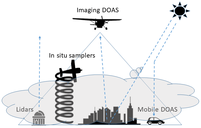
Figure 4Geometry of the main measurements performed during the AROMAT campaigns. The Imaging DOAS instruments map the NO2 and SO2 VCDs at 3 km altitude above the target area, while the in situ samplers measure profiles of trace gases and aerosols. Ancillary ground measurements include Mobile DOAS to quantify trace gases VCDs and lidars to measure the aerosol optical properties.
We used two small tropospheric aircraft: the Cessna-207 from FUB, and the Britten-Norman Islander (BN-2) from INCAS. The Cessna was dedicated to remote sensing. It mainly performed mapping flights at 3 km a.s.l. for the airborne imagers, while parts of the ascents and descents were used to measure aerosol extinction profiles with the FUBISS-ASA2 instrument. The BN-2, which was only used during AROMAT-2, was dedicated to in situ measurements around Bucharest between the surface and 3000 m a.s.l. In AROMAT-2, there was also an ultralight aircraft used by UGAL for nadir DOAS observations in the Jiu Valley. The ultralight aircraft typically flew between 600 and 1800 m a.s.l. Two UAVs operated by INCAS and UGAL flew during AROMAT-1. These measurements were not repeated during AROMAT-2 since the coverage of the UAVs was too limited in both the horizontal and vertical directions. Finally, we also launched balloons carrying NO2 sondes from Turceni and performed Mobile DOAS measurements from several cars during both campaigns. The Supplement provides more details about the practical deployments during the campaigns.
2.4 The 2014 AROMAT campaign
The AROMAT-1 campaign took place between 1 and 13 September 2014. The operations started in Bucharest with the continuous observations from the Romanian Atmospheric 3D Observatory (RADO, Nicolae et al., 2010) in Măgurele and synchronised car-based Mobile DOAS observations around the Bucharest ring road and within the city. During the first 2 d of the campaign, the INCAS UAV flew from the Clinceni airfield with two different aerosol payloads (the TSI Dust Trak DRX and TSI aerosol particle sizer) up to an altitude of 1.2 km a.s.l. The Cessna was not allowed to fly over the city but performed loops above the ring road at a low altitude of 500 m a.s.l. The remote sensing measurements stopped on 4 September due to bad weather. On 5 and 6 September, we collected data only from the ground and in broken cloud conditions.
On 7 September 2014, part of the campaign crew moved to the Jiu Valley. We installed the INOE mobile laboratory (in situ monitors, MILI lidar, and ACSM) in Turceni and performed the first UAV flights around the power plant on 8 September 2014 with the NO2 sonde and SWING. On the same day, in Bucharest the Cessna flew above the city with AirMAP and Mobile DOAS operated on the ground. On the following day, 9 September 2014, the Cessna did a second mapping of Bucharest, and we started to launch balloons from Turceni, carrying the NO2 sonde. In total, 11 balloons were launched between 8 and 12 September 2014, out of which 10 led to successful measurements. Technical issues with both the UAV and the Cessna interrupted the flights for a couple of days. The UAV operations started again with a SWING flight on 10 September 2014. On 11 September 2014, the AirMAP and SWING flew in coincidence above Turceni, on the Cessna and the UAV, respectively, and we performed two more short SWING-UAV flights. On 12 and 13 September, we performed two more Cessna flights above the Jiu Valley, but the weather conditions were degrading. During the entire second week of the campaign, Mobile DOAS measurements were performed in Turceni and around the other power plants of the Jiu Valley.
Table S5 in the Supplement summarises the main measurement days during AROMAT-1, specifying if the measurements were taken in Bucharest or in the Jiu Valley. The “golden days” of the AROMAT-1 campaigns are 2, 8, and 11 September 2014. These days are particularly interesting due to good weather conditions and coincident measurements. On 2 September 2014, we operated the three Mobile DOAS together around Bucharest. On 8 September 2014, we flew AirMAP above Bucharest with the UGAL and MPIC Mobile DOAS on the ground. Finally, on 11 September 2014, SWING and AirMAP were time coincident above the Turceni power plant, and two balloons sampled the vertical distribution of NO2.
2.5 The 2015 AROMAT-2 campaign
The AROMAT-2 campaign took place between 17 and 31 August 2015. We started in Bucharest with car-based Mobile DOAS measurements and observations at RADO. The INOE mobile lab was installed in Turceni on 19 August 2015, followed by an SO2 camera (instrument described in Kern et al., 2015; Stebel et al., 2015) and NO2 camera (Dekemper et al., 2016). Poor weather conditions limited the relevance of the measurements during the first days of the campaign. Two Mobile DOAS teams in Bucharest moved from Bucharest to the Jiu Valley on 23 August 2015. From then, the weather was fine until the end of the campaigns, and valuable data were collected during all days between 24 and 31 August 2015.
In the Jiu Valley, the crew was based in Turceni and most of the static instruments were installed at a soccer field. Alongside the INOE mobile lab with in situ samplers, the scanning lidar, SO2 cameras, and the NO2 camera pointed to the power plant plume. The NO2 camera acquired images until 25 August 2015. The car-based Mobile DOAS operated in the Valley between the different power plants. From 24 August, the SO2 cameras were split: one of them stayed in the soccer field, the two others were installed at several points around Turceni. Also on 24 August, the UGAL ultralight took off from Craiova and flew to the Jiu Valley until Rovinari, carrying the ULM-DOAS instrument. This experiment was repeated on 25, 26, and 27 August. On 28 August 2015, the Cessna flew above Turceni with AirMAP and SWING.
In Bucharest, the BN-2 first flew on 25 August 2015. It took off from Strejnicu and carried various in situ instruments (the TSI nephelometer and aerosol particle sizer, the NO2 CAPS, the PICARRO, and the KNMI NO2 sonde) and flew in a loop pattern at 500 m a.s.l. around the city ring road. After this test flight, the aircraft performed six flights between 27 and 31 August 2015, which included soundings around Băneasa and Măgurele, up to 3300 m a.s.l. On 30 and 31 August 2015, the Cessna mapped the city of Bucharest, performing two flights per day. It also performed soundings to measure AOD profiles with the FUBISS-ASA2 instrument (Zieger et al., 2007).
Table S6 in the Supplement summarises the measurements of the AROMAT-2 campaign, specifying whether the measurements were taken in Bucharest or in the Jiu Valley. Compared to the AROMAT-1 campaign, a larger number of instruments took part and a larger number of “golden days” occurred. All of the days between 24 and 31 August 2015 led to interesting measurements. Regarding intercomparison exercises for the airborne imagers, the best days are 28 August 2015 (Jiu Valley) and 31 August 2015 (Bucharest).
This section presents selected findings related to tropospheric NO2, SO2, and H2CO in the two target areas. The Supplement gives details about the instruments involved in these observations and presents additional measurements in Bucharest and the Jiu Valley.
3.1 Bucharest
3.1.1 Horizontal distribution of NO2
Figure 5 presents two maps of the AROMAT NO2 measurements performed with the AirMAP, CAPS, and MPIC Mobile DOAS instruments above Bucharest, on 30 (Sunday afternoon, Figure 5a) and 31 (Monday afternoon, Figure 5b) August 2015. AirMAP is a remote sensing instrument that mapped the NO2 VCDs from the Cessna at 3 km a.s.l. and produced the continuous map. The CAPS is an in situ instrument, it was operated on the BN-2, sampled the air at 300 m a.s.l., and performed vertical soundings above Măgurele. The MPIC Mobile DOAS mainly drove along the Bucharest ring road.
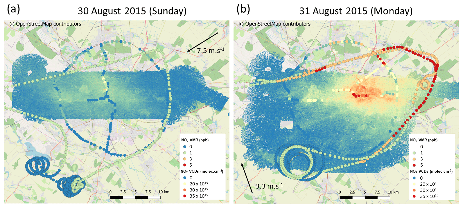
Figure 5Measurements of NO2 VCDs and volume mixing ratios in Bucharest on 30 (Sunday, a) and 31 (Monday, b) August 2015 with AirMAP (continuous map), the CAPS (black-rimmed circles), and the MPIC Mobile DOAS (plain colour circles).
The datasets of Fig. 5 reveal large differences of NO2 amounts on Sunday 30 August 2015 compared to Monday 31 August 2015. On Sunday afternoon, the NO2 VCDs peak around 1.5×10¹⁶ molec. cm−2. On Monday, the NO2 plume spread from the centre to the northeast of the city. The observed NO2 VCDs were smaller than the detection limit upwind and reach up to 3.5×10¹⁶ molec. cm−2 inside the plume. The NO2 volume mixing ratio (VMR) measured with the CAPS was close to the detection limit on Sunday while it reached 5 ppb inside the plume on Monday 31 August 2015. Note that the time difference between both measurements partly explain the systematic differences between AirMAP and the MPIC Mobile DOAS at the eastern part of the ring road on 31 August 2015. Meier (2018) compared the two instruments during the morning flight (between 07:00 and 09:30 UTC), which includes more simultaneous observations. Considering only co-located measurements with a maximum time difference of 45 min, the comparison reveals a good agreement when averaging the forward and backward-looking Mobile DOAS NO2 VCDs. The MPIC/AirMAP slope is 0.93 while the correlation coefficient of 0.94. The remaining discrepancy may be explained by air mass factor (AMF) errors and differences in time and horizontal sensitivity. Figure S2 in the Supplement presents this quantitative comparison.
Figure 6 presents co-located CAPS and AirMAP NO2 measurements on 31 August 2015. The BN-2 carrying the CAPS flew from Măgurele to the East of Bucharest, remaining outside the city ring at 300 m a.s.l. between 12:30 and 12:55 UTC, while AirMAP on board the Cessna was mapping the city between 12:00 and 13:30 UTC. We extracted the AirMAP NO2 VCDs at the position of the CAPS observations. The figure confirms that the two instruments detected the plume at the same place. This suggests that along this portion of the flight, which was inside the plume but outside the city, the NO2 VMR measured at 300 m a.s.l. may be used as a proxy for the NO2 VCD. Indeed, the boundary layer height (BLH) was about 1500 m (Fig. S8 in the Supplement and the discussion therein) during these observations. Assuming a constant NO2 VMR of 3.5 ppb in the boundary layer leads to a NO2 VCD of 1.4×10¹⁶ molec. cm−2. This estimate is close to the AirMAP NO2 VCD observed in the plume (Fig. 6). When measured at 300 m a.s.l., the NO2 VMR thus seems a good estimate of its average within the boundary layer. Note that this finding is specific to the configuration in Bucharest where we flew at 10 km from the city centre and does not apply to our measurements in the exhaust plume of the Turceni power plant (Fig. 9). Future campaigns should include vertical soundings inside the Bucharest plume to further investigate its NO2 vertical distribution.
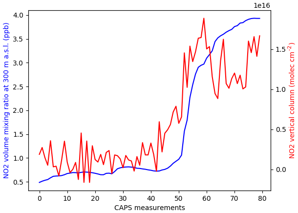
Figure 6Volume mixing ratio and VCDs of NO2 in and out of the pollution plume of Bucharest, as measured with the CAPS (on the BN-2, 12:30–12:55 UTC) and AirMAP (on the Cessna, 12:00–13:30 UTC) during the afternoon flights on 31 August 2015. Note that the plot shows the VCDs extracted at the position of the CAPS measurements.
3.1.2 Horizontal distribution of H2CO
Figure 7 shows the H2CO and NO2 VCDs measurements from the IUP-Bremen nadir instrument operated on board the Cessna on 31 August 2015 (morning flight), together with the MPIC Mobile DOAS measurements. The airborne data shown correspond to the second overpass (07:46–08:23 UTC), while the Mobile DOAS were recorded between 08:13 and 10:00 UTC. The H2CO VCDs range between and molec. cm−2, a maximum observed inside the city. We estimated the H2CO reference column for the airborne data using the Mobile DOAS measurements. Both NO2 and H2CO are in good agreement when comparing their distributions as seen from the airborne and ground-based instruments. However, if the highest H2CO VCDs are found above the Bucharest city centre, they are not coincident with the NO2 maximum, as can be seen when comparing Fig. 7a and b, e.g. on the second Cessna flight line from the north.
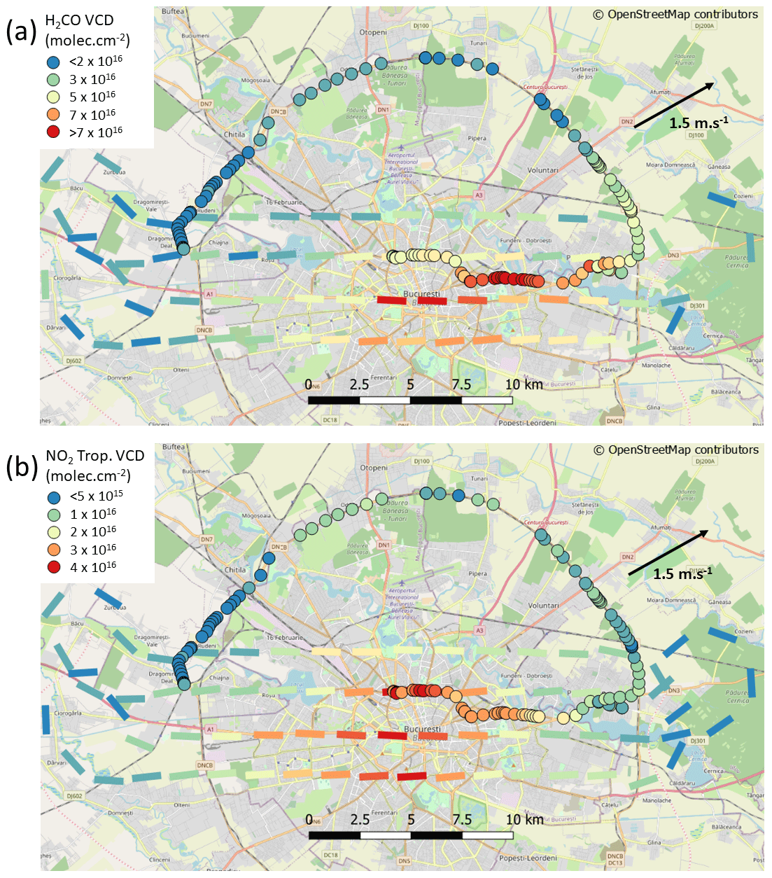
Figure 7Horizontal distribution of tropospheric H2CO and NO2 VCDs measured on 31 August 2015 with the IUP-Bremen nadir-only compact spectrometer from the Cessna (flight tracks, 07:46–08:23 UTC) and with the MPIC Mobile DOAS (coloured circles, 08:13–10:00 UTC).
The H2CO hotspot observed above Bucharest is mainly anthropogenic. Indeed, biogenic emissions typically account for 1 to 2×10¹⁶ molec. cm−2 (Jean-François Müller, personal communication, 2019), in agreement with the background VCDs measured by the Mobile DOAS along the Bucharest ring. During the measurements, the wind was blowing from the south and west. The difference between the NO2 and H2CO spatial patterns may be explained by the different origins of NOx compared to H2CO or by the formation time of H2CO through the oxidation of volatile organic compounds.
Anthropogenic hotspots of H2CO have already been observed, e.g. above Houston (Texas, USA), an urban area which includes significant emissions from transport and the petrochemical industry (Parrish et al., 2012; Nowlan et al., 2018). Nowlan et al. also deployed an airborne DOAS nadir instrument, they reported H2CO VCDs up to 5×10¹⁶ molec. cm−2 in September 2013.
3.2 The Jiu Valley
3.2.1 Spatial distribution of NO2
Figure 8 presents the horizontal distribution of the NO2 VCDs in the Jiu Valley measured with the MPIC Mobile DOAS on 23 August 2015 between 08:07 and 14:16 UTC. The figure shows elevated NO2 VCDs close to the four power plants listed in Table S1 of the Supplement, with up to 8×10¹⁶ molec. cm−2 downwind of Turceni and Rovinari. In comparison, the area east of Craiova is very clean, with typical NO2 VCDs under 1×10¹⁵ molec. cm−2.

Figure 8Tropospheric vertical column densities of NO2 measured with the MPIC Mobile DOAS instruments in the Jiu Valley on 23 August 2015 between 08:07 and 14:16 UTC.
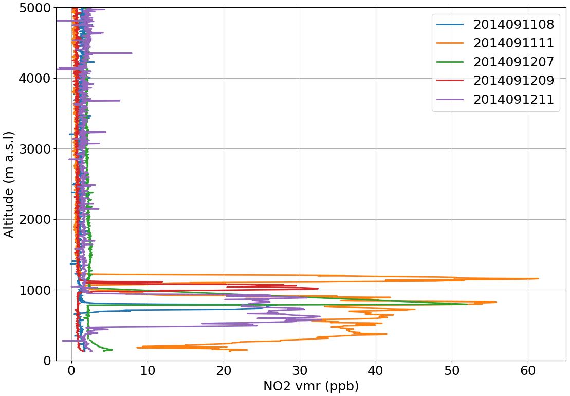
Figure 9Examples of NO2 sondes data from Turceni during AROMAT-1 (11 and 12 September 2014). The legend indicates the date, with the last two digits being the hour of launch (UTC).
The situation of Fig. 8 is characteristic of the conditions encountered in the Jiu Valley, with high NO2 VCDs observed to the north and west of the plants due to the prevailing wind directions. During both campaigns, we observed maximum NO2 VCDs reaching up to 1.3×10¹⁷ molec. cm−2, close to the plants with Mobile DOAS instruments.
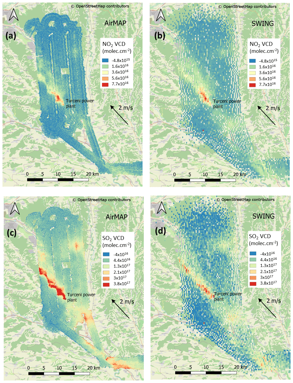
Figure 10AirMAP (a, c) and SWING (b, d) NO2 (a, b) and SO2 (c, d) VCDs above Turceni (28 August 2015).
Figure 10a and b show the AirMAP and SWING NO2 VCDs measured around the Turceni power plant on 28 August 2015. The two airborne instruments largely agree, detecting NO2 VCDs up to 8×10¹⁶ molec. cm−2 in the exhaust plume of the power plant. Figure S5 in the Supplement (upper panel) extracts the AirMAP and SWING NO2 VCDs along the path of the ground-based BIRA Mobile DOAS measurements and compares the three datasets. The airborne data correspond to three portions of flight lines recorded between 09:54 and 10:17 UTC. The BIRA Mobile DOAS instrument was sampling the plume during this time, and thus the maximum time difference is 23 min. This comparison confirms the good agreement with the airborne instruments but indicates that comparing airborne nadir-looking DOAS with ground-based zenith Mobile DOAS instruments is not straightforward in these conditions. Table S2 in the Supplement gives the typical AMFs used in this analysis for airborne and zenith-only Mobile DOAS. When observed with the Mobile DOAS, the plume shows higher NO2 VCDs and appears narrower than with the airborne instruments. This is partly related to air mass factor uncertainties, but they alone can not explain such a discrepancy. Close to the power plant, the plume is very thin and heterogeneous, which leads to 3D effects in the radiative transfer, as suggested in a previous AROMAT study (Merlaud et al., 2018). In these conditions, the 1D atmosphere of the radiative transfer models used to calculate the airborne AMFs may not be realistic enough and could bias the VCDs measured from the aircraft.
Figure 9 shows those AROMAT-1 NO2 sonde measurements above Turceni that detected the plume. The NO2 is not well mixed in the boundary layer, with maxima aloft and lower VMRs close to the surface. This is understandable so close to the source, as high-temperature NOx is emitted from the 280 m high stack. In these balloon-borne datasets, the observed maximum NO2 VMR is about 60 ppb inside the plume, and the NO2 VMR vanishes above 1200 m a.s.l. These results suggest that airborne measurements with the ULM-DOAS, which can fly safely at 1500 m a.s.l., can provide reliable measurements of the integrated column amount inside the plume.
3.2.2 Horizontal distribution of SO2
Figure 10c and d present the SO2 horizontal distributions measured around Turceni with AirMAP (Fig. 10c) and SWING (Fig. 10) on 28 August 2015. The maps show the plume from the Turceni plant transported in the northwest direction, and other areas with elevated SO2 VCDs to the east and south of Turceni. Meier (2018) presents these AirMAP SO2 observations in detail and compares them with SWING results. Figure S4 in the Supplement shows the corresponding time series of SWING and AirMAP SO2 'differential slant column densities (DSCDs). It is found that the AirMAP-derived SO2 columns inside the plume SO2 reach 6×10¹⁷ molec. cm−2 and that the AirMAP and SWING SO2 VCDs agree within 10 %. Moreover, for these airborne data, the SO2 horizontal distribution broadly follows that of NO2. The discrepancies can be explained by the different lifetimes of the two species.
As for NO2, it appears difficult to quantitatively relate the airborne and Mobile DOAS SO2 VCD observations in the close vicinity of the power plant. As shown in Fig. S5 of the Supplement (lower panel), the maximum SO2 VCD measured from the ground on the road close to the factory amounts to 1.3×10¹⁸ molec. cm−2, while from the aircraft the SO2 VCD reached 8×10¹⁷ molec. cm−2. Part of this difference can be explained by 3D effects on the radiative transfer, as is the case for NO2. As discussed below, it seems easier to compare the SO2 flux.
In this section, we develop the lessons learnt from our study for the validation of satellite observations of the three investigated tropospheric trace gases, namely NO2, SO2, and H2CO. For each molecule, we discuss the benefit of conducting such airborne campaigns as well as the choice of Romania as a campaign site. In the last part of the section, we also estimate the NOx and SO2 emissions from Bucharest and from the power plants of the Jiu Valley, using the different datasets of the campaigns.
4.1 Lessons learnt for the validation of space-borne NO2 VCDs
4.1.1 Number of possible pixels and dynamic range at the TROPOMI resolution
Regarding Bucharest, the mapped area of Fig. 5b virtually covers 43 TROPOMI near-nadir pixels. Averaging the high spatial resolution AirMAP NO2 VCDs within these 43 hypothetical TROPOMI measurements reduces the dynamic range of the observed NO2 field. The latter decreases from 3.5×10¹⁶ to 2.6×10¹⁶ molec. cm−2 (37 σ where σ is the required precision on the tropospheric NO2 VCD). Nevertheless, 33 of the 43 hypothetical TROPOMI pixels exhibits a NO2 VCD above the required 2σ random error for TROPOMI (1.4×10¹⁵ molec. cm−2).
Regarding the Jiu Valley, a similar exercise based on our measurements on 28 August 2012 (Fig. 10a and b) leads to 48 near-nadir TROPOMI pixels, out of which 35 would have a NO2 VCD above the 2σ TROPOMI error. The largest NO2 tropospheric VCD seen by TROPOMI would be around 2×10¹⁶ molec. cm−2 (29 σ for TROPOMI).
4.1.2 Characterisation of the reference measurements
Table 3 summarises the NO2 observations during the AROMAT campaigns. For each instrument, the table indicates the measured range of NO2 VCDs (or VMRs), the ground sampling distance and a typical detection limit and bias. Regarding DOAS instruments, we estimated the detection limits on the NO2 VCDs from typical 1σ DOAS fit uncertainties divided by typical air mass factors (AMF). Table S2 in the Supplement presents these typical AMFs and detection limits. The 1σ DOAS fit uncertainty is instrument specific and an output of the DOAS fitting algorithms. The AMF depends on the observation's geometry and atmospheric and surface optical properties. Uncertainties in the AMF usually dominate the systematic part of the error for the DOAS measurements. Therefore, for these instruments, the bias given in Table 3 corresponds to the uncertainty in their associated AMF.
Meier et al. (2017)Merlaud et al. (2018)Constantin et al. (2017)Bösch et al. (2016)Donner et al. (2015)Wagner et al. (2010)Constantin et al. (2013)Merlaud (2013)Sluis et al. (2010)Kebabian et al. (2005)Table 3Summary of the AROMAT measurements of NO2.
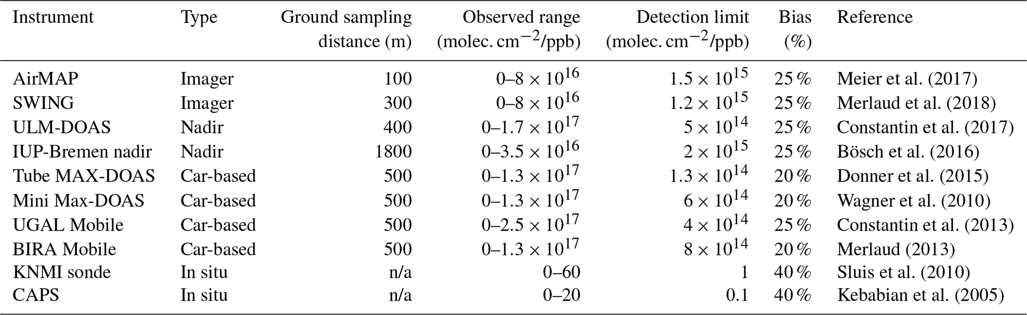
n/a: not applicable.
Combined with the ground sampling distance, the detection limit enables one to quantify the random uncertainty of a reference observation at the satellite horizontal resolution. Indeed, considering reference measurements averaged within a satellite pixel, the random error associated with the averaged reference measurements decreases with the square root of the number of measurements, following Poisson statistics. For instance, continuous mapping performed with SWING at a spatial resolution of 300×300 m2 inside a TROPOMI pixel of 3.5×5.5 km2 would lead to 214 SWING pixels. Averaging the NO2 VCDs of these SWING pixels would divide the SWING original uncertainty (1.2×10¹⁵ molec. cm−2) by , leading to 8.2×10¹³ molec. cm−2, about a tenth of the random error of TROPOMI (7×10¹⁴ molec. cm−2) given in Table 2.
However, the temporal variation of the NO2 VCDs further adds uncertainty to the reference measurements when comparing them with satellite data. The validation areas typically extend over tens of kilometres. At this scale, satellite observations are a snapshot in time of the atmospheric state, while airborne mapping typically takes 1 or 2 h.
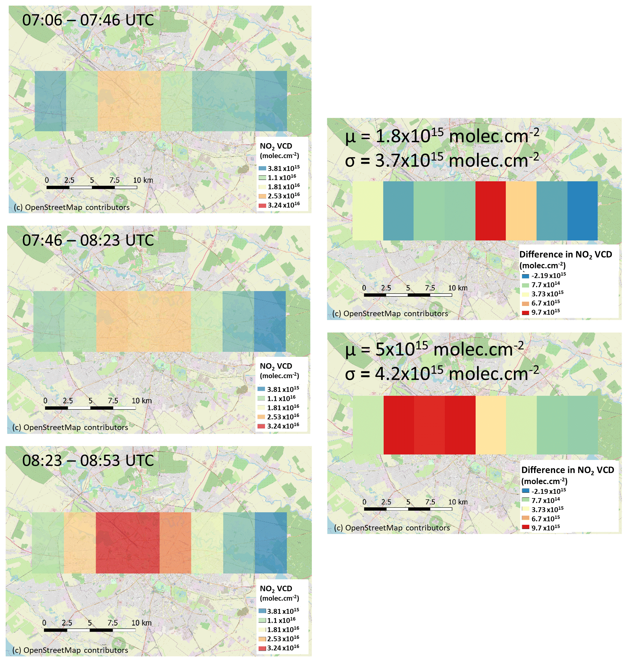
Figure 11AirMAP measurements of NO2 VCDs degraded at the TROPOMI resolution during three overpasses of the morning flight of 31 August 2015 (left column), together with the differences of these degraded NO2 VCDs for consecutive overpasses (right column). The right column also indicates the means (μ) and standard deviations (σ) of the two differences.
Figure 11 illustrates our estimation of the temporal variation of the NO2 VCDs, comparing consecutive AirMAP overpasses above Bucharest from the morning flight of 31 August 2015. During this flight, the Cessna covered the same area three times in a row between 07:06 and 08:52 UTC. Figure S3 in the Supplement presents the corresponding AirMAP and SWING NO2 DSCDs. For each AirMAP overpass, we averaged the NO2 VCDs at the horizontal resolution of TROPOMI (see previous section). The standard deviation of the differences between two averaged overpasses then indicates the random part of the NO2 VCDs temporal variation during an aircraft overpass. This standard deviation is 3.7×10¹⁵ and 4.2×10¹⁵ molec. cm−2, respectively, between the first and second and second and third overpasses. Hereafter, we used 4×10¹⁵ molec. cm−2 as the random error due to the temporal variation.
Clearly, the NO2 VCD temporal variation depends on characteristics of a given validation experiment, such as the source locations and the wind conditions during the measurements. The temporal variation also depends on the time of the day, and we base our estimate here on measurements around 11:00 LT, while the TROPOMI overpass is at 13:30 LT. In the studied case, however, this error source is larger for the reference measurements than the TROPOMI precision (7×10¹⁴ molec. cm−2). This is quite different from using static MAX-DOAS as reference. The latter is usually averaged within 1 h around the satellite overpass. Compernolle et al. (2020) quantify the temporal error for MAX-DOAS NO2 VCDs, typically ranging between 1 to 5×10¹⁴ molec. cm−2. In the next section, we investigate the effect of underestimating the temporal random error.
4.1.3 Simulations of validation exercises in different scenarios
We simulated TROPOMI validation exercises with the spatially averaged AirMAP observations described in Sect. 4.1.1. We considered these averaged AirMAP NO2 VCDs as the ground truth in simulated TROPOMI pixels, upon which we added Gaussian noise to build synthetic satellite and reference NO2 VCDs datasets. For the synthetic satellite observations, the noise standard deviation corresponded to the TROPOMI random error (the precision in Table 2). For the synthetic airborne observations, we added the aforementioned averaged airborne shot noise (e.g. 7×10¹³ molec. cm−2 for SWING) and temporal error (4×10¹⁵ molec. cm−2, which we assumed to be also realistic around Turceni) in quadrature. We then applied weighted orthogonal distance regressions to a series of such simulations to estimate the uncertainty of the regression slope. This led to slope uncertainties of about 6 % and 10 % in Bucharest and Turceni, respectively.
In a real-world validation experiment, this regression slope would quantify the combined biases of the two NO2 VCDs datasets (satellite and reference). These biases mainly originate from errors in the AMFs, resulting in particular from uncertainties in the NO2 and aerosol profiles, and on the surface albedo. To some extent, these quantities can be measured from an aircraft with the type of instrumentation deployed in the AROMAT activity. The ground albedo can be retrieved with the DOAS instruments by normalising uncalibrated airborne radiances to a reference area with known albedo (Meier et al., 2017) or by using a radiometrically calibrated DOAS sensor (Tack et al., 2019). The NO2 and aerosol profiles can be measured with in situ instruments such as a CAPS NO2 monitor and a nephelometer. For legal reasons, vertical soundings are difficult above cities. One can measure the NO2 and aerosol profile further down in the exhaust plume, once the latter is above rural areas. The conditions inside the city can be different, and this motivates the deployment of ground-based instruments, e.g. sun photometers and MAX-DOAS, inside the city.
Regarding uncertainties in the reference AMFs, the benefit of knowing the aerosol and NO2 profile appears when comparing the AMF error budget for airborne measurements above Bucharest (26 %, Meier et al., 2017) and above the Turceni power plant (10 %, Merlaud et al., 2018). In the latter case, there was accurate information on the local NO2 and aerosol profiles thanks to the lidar and the balloon-borne NO2 sonde, respectively. We used these two AMF uncertainties to estimate a total possible bias between reference and satellite observations.
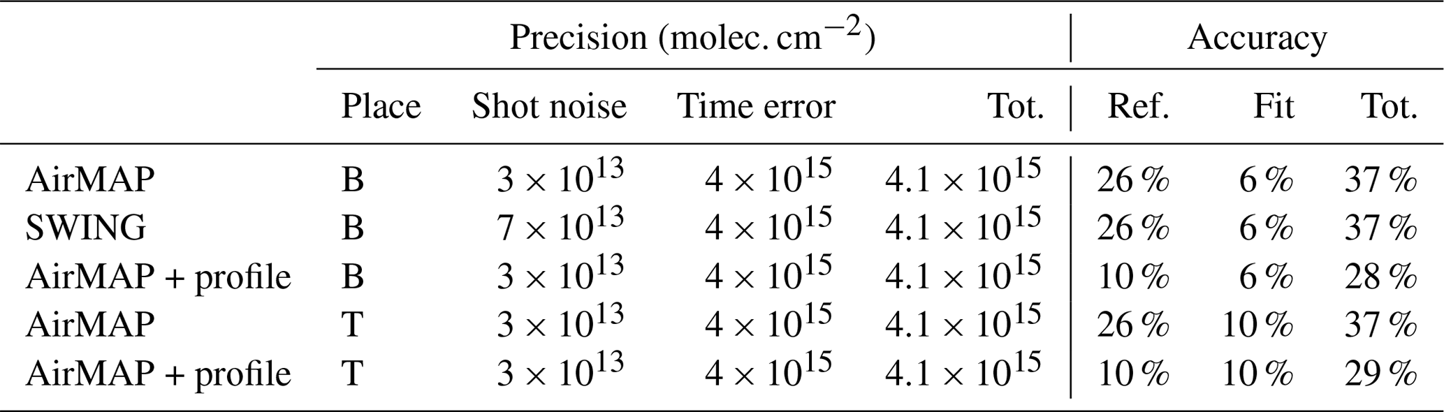
Table 6 presents total error budgets for different scenarios of validation exercises using reference airborne mapping to validate space-borne tropospheric NO2 VCDs. We estimated the random and systematic uncertainties between satellite and reference measurements with SWING and AirMAP, including (or not including) profile information on the aerosols and NO2 VMR, and for measurements over Bucharest or Turceni. Note that we considered 25 % for the satellite accuracy. The temporal error of the airborne measurements clearly dominates the total random error, making the differences in detection limit between AirMAP and SWING irrelevant for this application. Adding the profile information, on the other hand, reduces the total multiplicative bias from 37 % to 28 % or 29 % in Bucharest and Turceni. This quantifies the capabilities of such airborne measurements for the validation of the imaging capabilities of TROPOMI regarding the NO2 VCDs above Bucharest and the Jiu Valley.
Finally, it should be noted that these regression simulations assume a correct estimation of the temporal random error. Underestimating this error propagates in the fit of the regression slope. Figure 12 presents the possible effect of such an underestimation when the a priori random error of the reference measurements is set at 1×10¹⁵ molec. cm−2, again using the AirMAP observations of Fig. 5b as input data. As the dynamic range of the reference measurements increases with the applied error, the fitted slope decreases. For a true error of 4×10¹⁵, this leads for instance to an underestimation of the slope of about 5 %. This effect is small, but other sources of random error (e.g undersampling the satellite pixels) would add up in a real-world experiment. Wang et al. (2017) observed such a systematic decrease of the regression slope when averaging MAX-DOAS measurements within larger time windows around the satellite overpass.
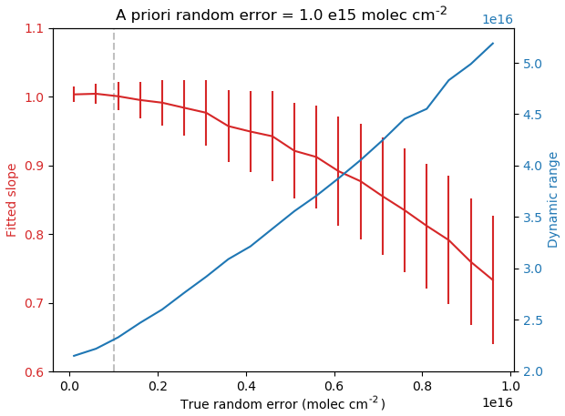
Figure 12Effect of an underestimation of the random error in a regression analysis simulating TROPOMI validation using airborne mapping as reference measurements of NO2 VCDs. The dynamic range (blue line) of the reference measurements increases with the applied random error. For the considered a priori random error (dashed vertical line, 1×10¹⁵ molec. cm−2), this leads to an underestimation of the regression slope (red line). These simulations use the AirMAP data of 31 August 2015 (afternoon flight).
4.2 Lessons learnt for the validation of space-borne H2CO VCDs
Table 4 is similar to Table 3 but for H2CO, which we only measured in significant amounts in and around Bucharest.
Bösch et al. (2016)Donner et al. (2015)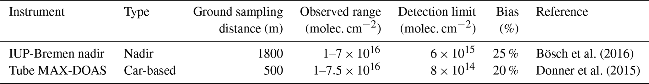
The background level of the H2CO VCD around the city is around 1×10¹⁶ molec. cm−2, and the anthropogenic increase in the city centre is up to 7×10¹⁶ molec. cm−2 (Fig. 7). The background falls within the TROPOMI H2CO spread (1.2×10¹⁶ molec. cm−2), and Fig. 7 indicates that the extent of the urban hotspot only corresponds to a few TROPOMI pixels, with a maximum at 6 σ. This limits the relevance of individual mapping flights for the validation of H2CO, yet systematic airborne measurements would improve the statistics. The information on the H2CO horizontal variability is nevertheless useful, as it justifies the installation of a second MAX-DOAS in the city centre, in addition to background measurements outside the city. Indeed, long-term ground-based measurements at two sites would be useful to investigate seasonal variations of H2CO, as already demonstrated at other sites (De Smedt et al., 2015). Averaging the H2CO over a season would reduce the random errors of the satellite measurements and could reveal the horizontal variability of H2CO from space. The H2CO hotspot around Bucharest seems to be visible in the TROPOMI data of summer 2018 (Isabelle De Smedt, personal communication, 2019).
Getting information on the profile of H2CO during an airborne campaign may also help us to understand the differences between ground-based and space-borne observations. This could be done by adding an in situ H2CO sensor, such as the In Situ Airborne Formaldehyde instrument (ISAF, Cazorla et al., 2015) or the COmpact Formaldehyde FluorescencE Experiment (COFFEE, St. Clair et al., 2017), to the BN-2 instrumental set-up.
4.3 Lessons learnt for the validation of space-borne SO2 VCDs
Table 5 is similar to Table 3 but for SO2, which we only measured in significant amounts in the Jiu Valley. The higher bias of the airborne measurements for SO2 compared to NO2 is due to the albedo. The latter is lower in the UV, where we retrieve SO2, which leads, for the same albedo error, to a larger AMF uncertainty (e.g. Merlaud et al., 2018, Fig. 10).
Meier et al. (2017)Merlaud et al. (2018)Constantin et al. (2017)Donner et al. (2015)Wagner et al. (2010)Constantin et al. (2013)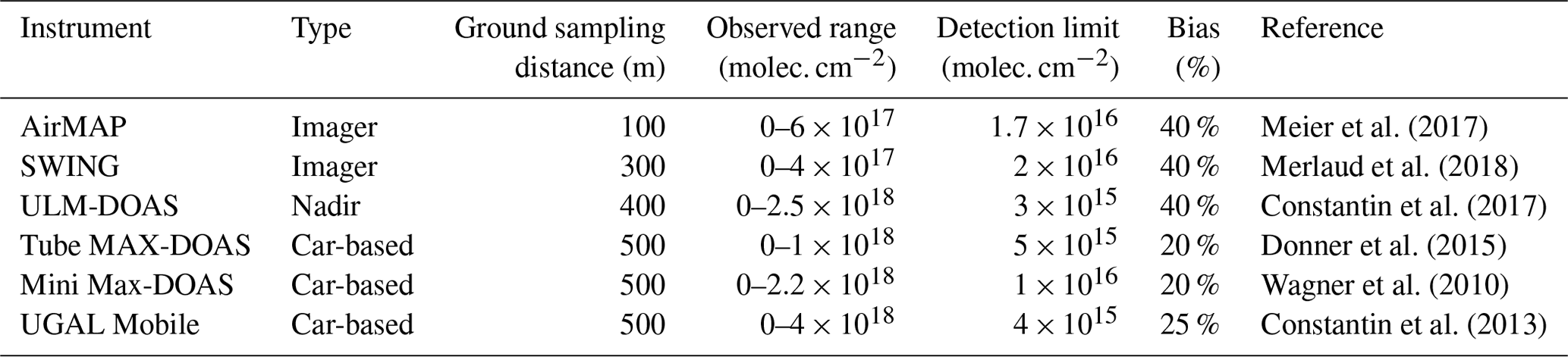
Table 6Total simulated error budget for the validation of space-borne NO2 VCD validation using airborne mapping at different resolutions, with or without profile information.
Averaging the SO2 VCDs from the airborne mapping of Fig. 10 at the TROPOMI resolution leads to 30 near-nadir TROPOMI pixels above a 2σ error of 5.4×10¹⁶ molec. cm−2. The maximum SO2 tropospheric VCD seen by TROPOMI would be 2.4×10¹⁷ molec. cm−2 (7 σ). This tends to indicate that airborne mappings of SO2 VCDs above large power plants could help to validate the horizontal variability of the SO2 VCDs measured from space to a limited extent in the AROMAT conditions due to the small dynamic range (7 σ). As for H2CO, systematic airborne measurements would improve the statistics.
However, it would be difficult to quantify the bias of the satellite SO2 VCD with AROMAT-type of airborne measurements. Adding in quadrature, the biases of the SO2 VCDs for airborne measurements (40 %, Table 5) and for TROPOMI (30 %, Table 2) already lead to a combined uncertainty of 50 %, without considering any temporal variation or regression error. This best-case scenario is already at the upper limit of the TROPOMI requirements for tropospheric SO2 VCDs (Table 2).
Similar to H2CO, the validation of the satellite-based SO2 measurements should thus rely on ground-based measurements, enabling us to improve the signal-to-noise ratio of the satellite and reference measurements by averaging their time series. An additional difficulty for validating SO2 VCDs emitted by a power plant arise from the spatial heterogeneity of the SO2 field around the point source, which renders ground-based VCDs measurements complicated.
On the other hand, Fioletov et al. (2017) presented a method to derive the SO2 emissions from OMI data and validated it against reported emissions. The SO2 fluxes can be measured locally in several ways, and we tested some of them during AROMAT-2 (see Sect. 4.4.2 below). To validate satellite-derived SO2 products in Europe, it thus seems possible to compare satellite and ground-based reference SO2 fluxes. Theys et al. (2019) already validated TROPOMI-derived volcanic SO2 fluxes against ground-based measurements. In this context, a SO2 camera pointing to the plant stack would be a valuable tool, since it could be permanently installed and automated. One advantage of such a camera compared to the other tested remote-sensing instruments, besides its low operating cost, is that it derives the extraction speed from the measurements, avoiding dependence on low-resolution wind information. The next section presents the SO2 fluxes derived with such a camera during the 2015 campaign.
Note that the SO2 VCDs measured on 28 August 2015 around Turceni may be higher than in standard conditions due to a temporary shutdown of the desulfurisation unit, which was reported by local workers. SO2 VCDs in the area seem to have decreased (D. Constantin, personal communication). The first reported TROPOMI SO2 measurements above the area pinpoint other power plants in Serbia, Bosnia and Herzegovina, and Bulgaria (Fioletov et al., 2020). For validation studies, it would be worth installing automatic SO2 cameras around these plants until they are equipped with FGD units.
4.4 Emissions of NOx and SO2 from Bucharest and the Jiu Valley
This section presents estimates of the NOx and SO2 fluxes from Bucharest and the power plants in the Jiu Valley, combining our different 2014 and 2015 measurements and comparing them with available reported emissions. Campaign-based estimates of NOx emissions from large sources are relevant in a context of satellite validation since the high resolution of TROPOMI enables us to derive such emissions on a daily basis (Lorente et al., 2019). Regarding SO2, as discussed in the previous section, the low signal-to-noise ratio of the satellite measurements implies averaging for several months to derive a SO2 flux (Fioletov et al., 2020), yet campaign measurements are useful to select an interesting site and test the ground-based apparatus and algorithms.
The comparisons with reported emissions should not be overinterpreted since we compare campaign-based flux measurements performed during a few days during daytime with reported emissions that represent yearly averages. Nevertheless, they give interesting indications about the operations of the FGD units of the power plants and possible biases in emission inventories.
Our flux estimates are all based on optical remote sensing measurements. They involve integrating a transect of the plume along its spatial extent and multiplying the outcome by the plume speed, which may correspond to the stack exit velocity (camera pointing to the stack) or to the wind speed (Mobile DOAS and Imaging DOAS). We refer the reader to previous studies for the practical implementations. Ibrahim et al. (2010) presented the method we used for Bucharest, where we encircled the city with the Mobile DOAS. Meier et al. (2017) presented the AirMAP-derived flux estimations, while Johansson et al. (2014) derived industrial emissions from a car-based Mobile DOAS instrument as we did for the Turceni power plant. Constantin et al. (2017) presented the fluxes based on the ULM-DOAS measurements. Regarding the SO2 cameras, they are now commonly used to monitor SO2 emissions from volcanoes (see McGonigle et al., 2017, and references therein), but their capacity to measure SO2 fluxes from power plants has been demonstrated as well (e.g. Smekens et al., 2014).
4.4.1 NOx flux from Bucharest
We estimated NOx fluxes from the Bucharest urban area using the NO2 VCDs measured with the UGAL Mobile DOAS systems along the external ring and the wind data on 8 September 2014 and 31 August 2015. We derived the wind direction from the maxima of the NO2 VCDs in the DOAS observations. For the wind speed, we took 1.1 m s−1 on 8 September 2014, the value Meier (2018) used for the AirMAP-derived flux, which originates from meteorological measurements at Băneasa airport. On 31 August 2015, we used the ERA5 wind data (C3S, 2017) at the time when the Mobile DOAS crossed the NO2 plume (15:00 UTC). The ERA5 database indicates a constant wind speed between 1000 and 900 hPa of 1.2 m s−1. Finally, similar to Meier (2018), we took a ratio of 1.32 for the NOx to NO2 ratio and estimated the chemical loss of NOx with a lifetime of 3.8 h and an effective source location in the centre of Bucharest.
Table 7 presents the AirMAP- and Mobile DOAS-derived NOx fluxes from Bucharest, ranging between 12.5 and 17.5 mol s−1. On 8 September 2014, the Mobile DOAS and airborne observations were coincident. Their estimated NOx fluxes agree within 20 %. This gives confidence in the flux estimation, yet one should keep in mind that the same wind data was used for both estimations. Meier (2018) estimated the uncertainties on the AirMAP-derived NOx flux to be around 63 %, while the uncertainty of Mobile DOAS-derived NOx flux typically range between 30 % and 50 % (Shaiganfar et al., 2017).
Table 7NOx emissions from Bucharest estimated from the AROMAT measurements. Note that we use UGAL and MPIC Mobile DOAS measurements for the estimates on 8 September 2014 and 31 August 2015, respectively.
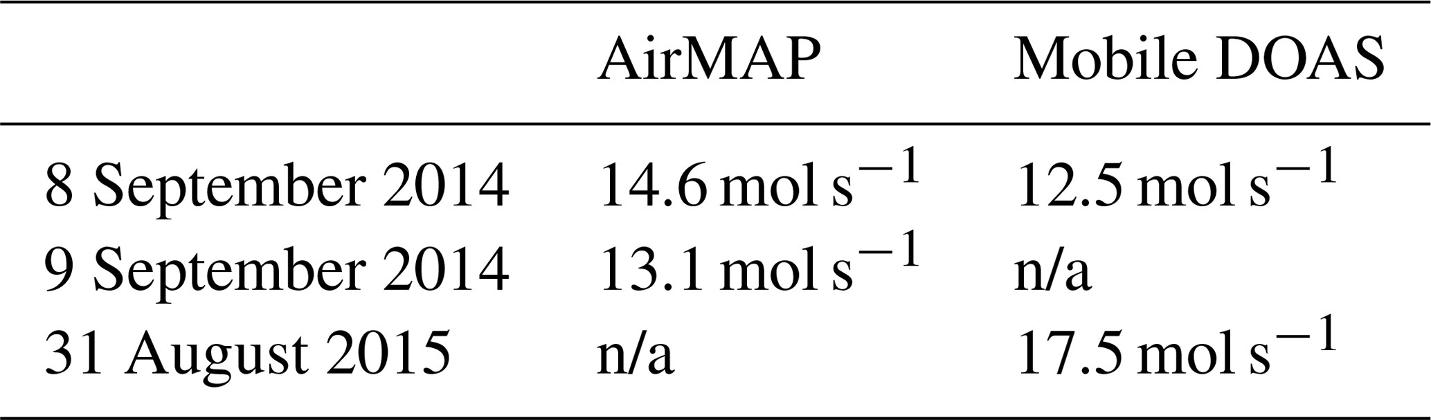
n/a: not applicable.
We compared our measured NOx fluxes with the European Monitoring and Evaluation Programme inventory (EMEP, https://www.ceip.at/, last access: 8 October 2020). In practice, we summed the EMEP gridded yearly NOx emissions between 44.2 and 44.6∘ N and between 25.9 and 26.3∘ E, and we assumed that the emissions are constant during 1 year. This led to NOx emissions of 6.14 and 6.33 mol s−1 for 2014 and 2015. Studying the reported emissions from several European cities, including Bucharest, Trombetti et al. (2018) mentions that the EMEP emissions are well below other inventories for all the pollutants. We thus also compared our flux with the Emissions Database for Global Atmospheric Research (EDGAR v4.3.2, Crippa et al., 2018), which is only available until 2012. The same method led to a NOx flux of 18.4 mol s−1, compared with the 2012 EMEP NOx emissions of 7.1 mol s−1. Based on summer measurements, the AROMAT-derived NOx emissions do not include residential heating. The latter ranges between 10 % and 40 % of the total NOx according to Trombetti et al. (2018). This tends to confirm that the EMEP inventory underestimates the NOx emissions for Bucharest.
4.4.2 NOx and SO2 fluxes from the power plants in the Jiu Valley
Figure 13 presents a scatter plot of the slant columns of NO2 and SO2 for the ultralight flight of 26 August 2015, which detected the four exhaust plumes of the Valley between 08:31 and 11:04 UTC. Two regimes are visible in the SO2 to NO2 ratio. When considering the longitude, the low SO2 to NO2 ratio (1.33) appears to correspond to the Rovinari exhaust plume, while the other power plants exhibit a higher ratio (13.55). The low ratio observed at Rovinari corresponds to the FGD units operating at this power plant.
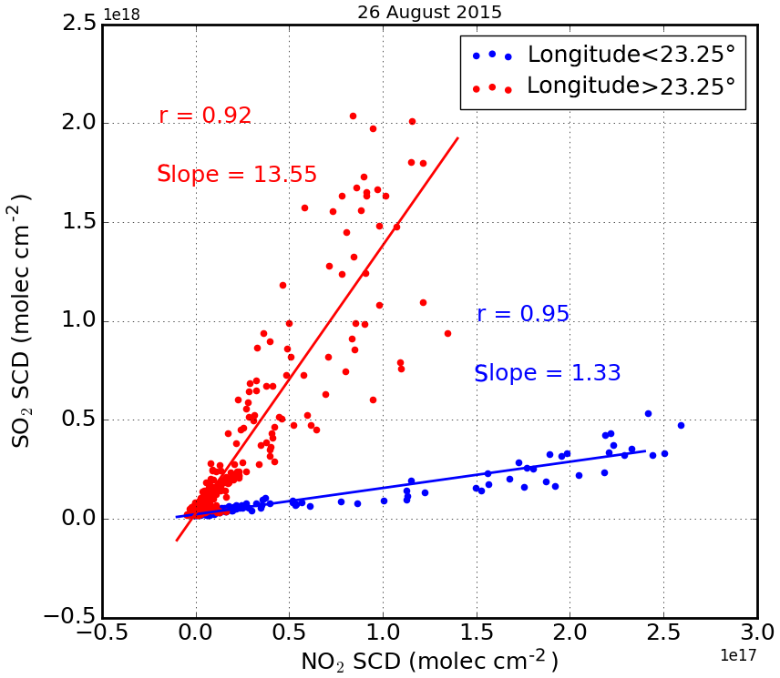
Figure 13SO2 and NO2 SCDs measured from the ULM-DOAS above the Jiu Valley on 26 August 2015 between 08:31 and 11:04 UTC. Blue dots indicate the measurements above Rovinari, whereas the red dots are for all of the other plants.
We estimated the NOx and SO2 flux from the power plants using several instruments: a Mobile DOAS, the ULM-DOAS, and the SO2 camera. For the DOAS instruments, we inferred the wind direction from the plume position and we retrieved the wind speed from the ERA5 database. Considering the observed vertical extent of the plume downwind of Turceni (Fig. 9), we took the wind speed at 950 hPa (ca. 500 m a.s.l.).
Figure 14 presents the ULM-DOAS-estimated fluxes of NOx and SO2 from the power plants in Turceni, Rovinari, and Craiova for the flight on 26 August 2015. The figure also shows the reported emissions from the European Environment Agency (EEA) large combustion plants database (EEA, 2018), assuming constant emissions throughout the year. Turceni appears to be the largest SO2 source (78 mol s−1), while Rovinari is the largest NOx source (8 mol s−1).
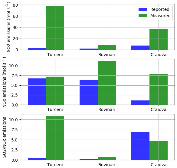
Figure 14SO2 and NOx fluxes from three power plants of the Jiu Valley, as (1) measured with the ULM-DOAS on 26 August 2015 (green bars) and (2) estimated from the reported emissions of 2015 assuming constant emissions throughout the year (blue bars). Uncertainties on the ULM-DOAS-derived fluxes are around 60 %.
It is difficult to interpret the discrepancies between those measured fluxes and the yearly reported emissions since we observed large variations in the instantaneous emissions with the SO2 camera (see below and Fig. 15). However, the ratio of the two fluxes appears interesting, since we can assume its relative stability. This ratio for a given power plant depends on whether or not a desulfurisation unit is operational at the plant. In Fig. 14, Turceni appears to have both the largest measured ratio and the largest discrepancy between the measured and reported ratios. This is consistent with a temporary shutdown of the desulfurisation unit of the Turceni power plant, as was reported by the plant workers during the campaign. The ULM-DOAS measurements on 25 August 2015 (shown in Fig. S11 the Supplement), which also sampled the Işalniţa plume, are consistent with those of 26 August 2015. These measurements enable us to estimate total NOx and SO2 fluxes to be about 22 and 147 mol s−1, respectively.
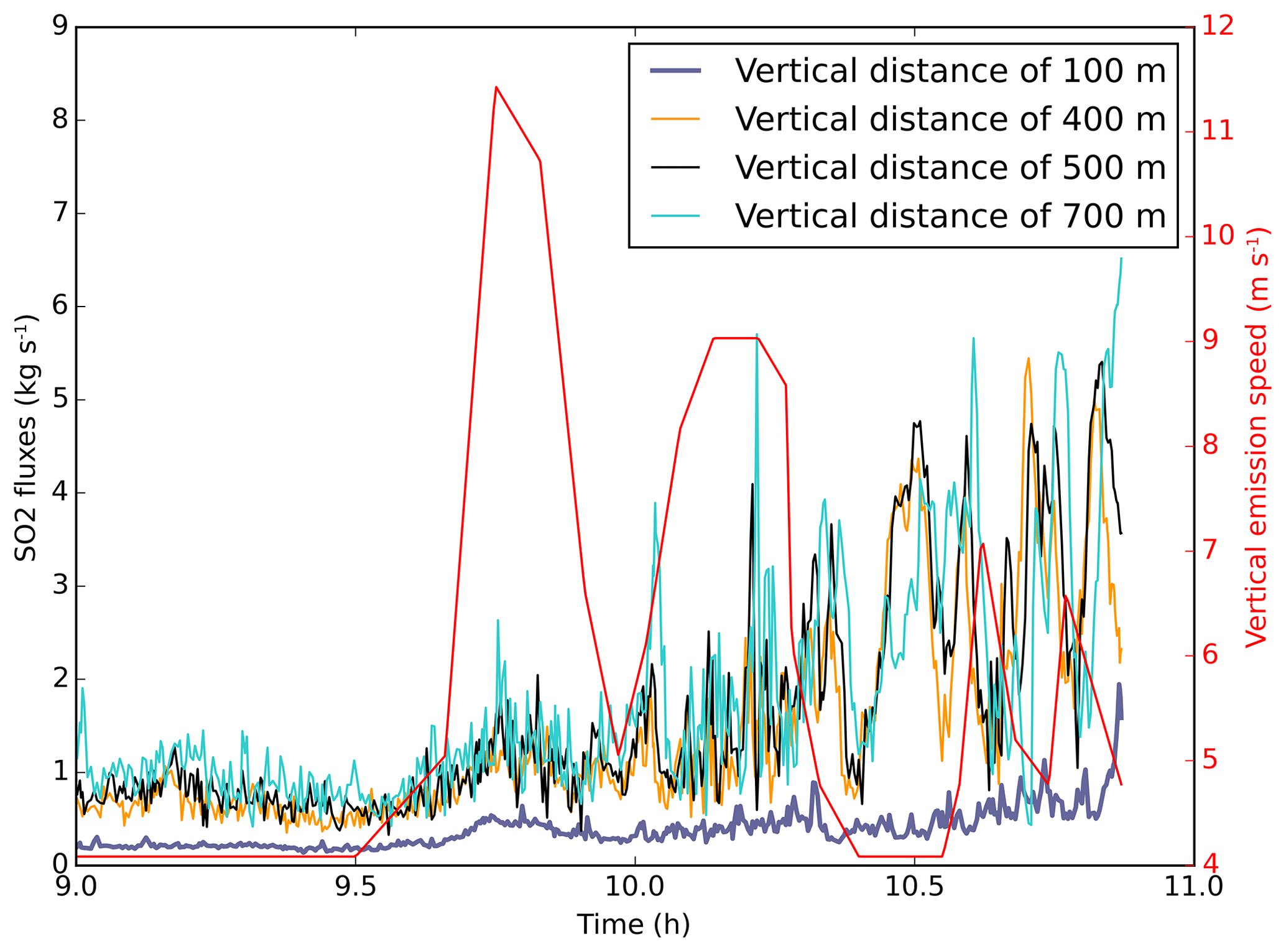
Figure 15SO2 fluxes from the Turceni power plant on 28 August 2015. They were estimated with the Envicam2 SO2 camera for four transverses at vertical altitudes above the stack of 100, 400, 500, and 700 m. The red line shows the estimated plume speed (m s−1).
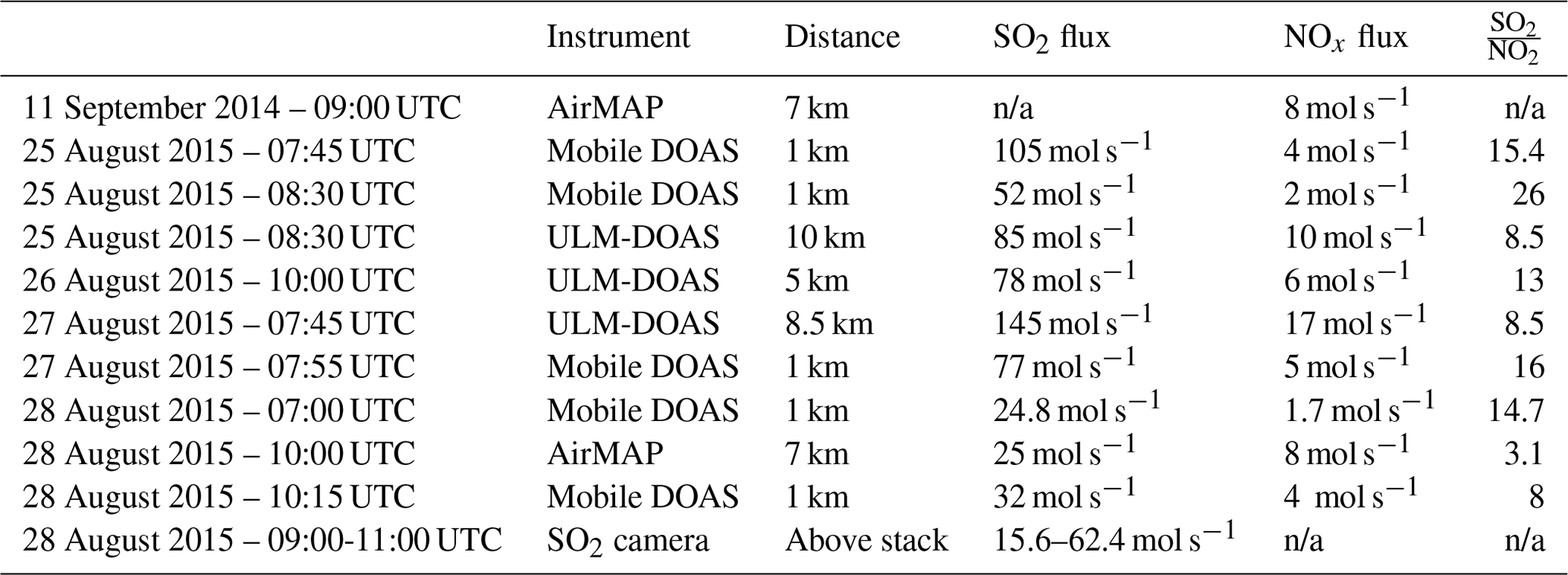
Table 8NOx and SO2 emissions from the Turceni power plant estimated from the AROMAT measurements.
n/a: not applicable.
Table 8 focuses on the Turceni power plant and lists all estimates of the NOx and SO2 emissions from this source. Meier (2018) estimated the NOx flux from the Turceni power plant using the AirMAP measurements of 2014 and 2015. This leads to similar values for the two flights on 11 September 2014 and 28 August 2015 of about 8 mol s−1. On this second day, the UGAL Mobile DOAS crossed the plume along the road in front of the power plant. These ground-based measurements lead to a NO2 flux of 2.2 mol s−1; much lower than the aforementioned AirMAP-derived value. However, Meier (2018) calculated the latter based on AirMAP measurements at 3.5 km from the source. At shorter distances, the AirMAP estimated NO2 flux is smaller and close to the Mobile DOAS observations. This is probably related to the fact that the NO∕NO2 ratio has not yet reached its steady-state value above the road where we performed the Mobile DOAS observations, which is only around 1 km from the stack. The agreement is better for SO2 (25 and 32 mol s−1). On 25 August 2015, we had a coincidence of ULM-DOAS and Mobile DOAS observations, and we observed a similar range of values. This gives us confidence in our estimate of the NOx flux from the aircraft but confirms that the nearby road is too close to the plant to estimate a meaningful NOx flux from Mobile DOAS NO2 observations. Note that the conversion of NO into NO2 is also visible right above the Turceni stack in the NO2 imager data of 24 August 2015, as appears in Fig. 6 of Dekemper et al. (2016).
Figure 15 presents a time series of the SO2 emissions from the Turceni power plant between 09:00 and 10:50 UTC on 28 August 2015. We derived SO2 fluxes at different altitudes above the stack using a UV SO2 camera that is an updated version of the Envicam2 system used during the SO2 camera intercomparison described by Kern et al. (2015). We converted the measured optical densities to SO2 column densities using simultaneous measurements with an integrated USB spectrometer (Lübcke et al., 2013). We estimated the stack exit velocity from the SO2 images, recorded with a time resolution of about 15 s, by tracking the spatial features of the plume. Dekemper et al. (2016) used a similar approach to derive the NO2 flux from NO2 camera imagery.
The SO2 fluxes retrieved for transverses at 400 to 700 m vertical distances above the stack agree on average with each other within 20 %. Emissions estimated 100 m above the stack are underestimated due to saturation (SO2 column densities above 2×10¹⁸ molec. cm−2) and high aerosol concentration close to the exhaust.
The SO2 emissions show large fluctuations. During the time of our observations they increased from 1 kg s−1 (15.6 mol s−1) to around 4±1 kg−1 (62.4 mol s−1). The images (Fig. S10 in the Supplement) also show a second, weaker source that emits SO2. This is probably the desulfurisation unit, which was reported to be turned on again on this day, after the temporary shutdown. Indeed, as appears in Table 8, the SO2∕NO2 ratio measured from AirMAP is lower than the ones measured from the ULM-DOAS during the previous days, and the same holds true for the Mobile DOAS measurements.
The two AROMAT campaigns took place in Romania in September 2014 and August 2015. They combined airborne and ground-based atmospheric measurements and focused on air-quality-related species (NO2, SO2, H2CO, and aerosols). The AROMAT activity targeted the urban area of Bucharest and the power plants of the Jiu Valley. The main aims were to test new instruments, measure the concentrations and emissions of key pollutants in the two areas, and investigate the concept of such campaigns for the validation of air quality satellite-derived products.
We have shown that the airborne mapping of tropospheric NO2 VCDs above Bucharest is potentially valuable for the validation of current and future nadir-looking satellite instruments. In the AROMAT conditions, airborne measurements were consistent with ground-based observations within 7 % and covered a significant part of the dynamic range of the NO2 tropospheric VCDs at an appropriate signal-to-noise ratio. Our simulations, based on campaign measurements and TROPOMI characteristics, indicate that we can constrain the accuracy of the satellite NO2 VCDs within 28 % or 37 %, depending on whether information on the aerosol and NO2 profile is available or not. This points to the importance of acquiring profile information to approach the TROPOMI optimal target accuracy for tropospheric NO2 VCDs (25 %).
A unique advantage of airborne mapping is its ability to validate the imaging capabilities of nadir-looking satellites. This feature becomes more important as the satellite horizontal resolutions reaches the suburban scale. Judd et al. (2019) pointed out the difficulty for static ground-based measurements to represent the NO2 VCDs measured from space in polluted areas, due to the horizontal representativeness error. This error cancels out by mapping the full extent of satellite pixels. The caveat is the temporal error, which can be larger than with static ground-based measurements. For a single morning flight above Bucharest, we have estimated the random part of this temporal error to be about 4×10¹⁵ molec. cm−2. In the AROMAT conditions, underestimating this error would lead to a low bias in the regression slope between satellite and airborne measurements. This temporal error varies with local conditions for a given experiment but the satellite air quality community should further investigate this effect. This indicates the usefulness of simultaneous ground-based measurements, which may also be useful to estimate the reference NO2 VCDs in the airborne observations. These conclusions for NO2 above Bucharest apply to other large polluted urban areas.
In addition to NO2, we also detected the signature of H2CO emissions in and around Bucharest, with an anthropogenic hotspot in the city centre. Due to the lower signal-to-noise ratio of the space-borne H2CO observations, it is difficult to use such daily measurements for satellite validation. We thus propose considering long-term ground-based MAX-DOAS measurements in the city for the validation of H2CO.
In the Jiu Valley, NO2 is clearly visible from both satellite and aircraft, and the VCDs are comparable in magnitude with the signal detected above Bucharest. However, it appears more complicated to quantitatively compare the NO2 VCDs datasets in the thick exhaust plumes of the power plants. These plants also emit SO2, but (as for H2CO) the low signal-to-noise ratio of satellite measurements reduces the validation relevance of individual airborne measurements.
In relation to the ideal validation study mentioned in the Introduction, the relevance of international airborne campaigns is generally limited by their typical time span of a couple of weeks, which is imposed by logistical and cost considerations. To overcome this limitation, we propose considering routine airborne mapping of NO2 VCDs by local aircraft operators and close to a well-equipped ground-based observatory. Such a set-up would reduce the fixed costs of the observations, which could then be allocated to flight hours in different seasons. Such an approach would combine the advantages of long-term ground-based and airborne measurements. In the longer term, high-altitude pseudo-satellites (HAPS) could provide the necessary routine measurements above selected supersites, as needed to validate the observations from future sensors in geostationary orbit.
The data of the two AROMAT campaigns are available upon request from ESA website (last access: 14 October 2020): https://earth.esa.int/eogateway/campaigns/aromat-i (AROMAT team, 2020).
The supplement related to this article is available online at: https://doi.org/10.5194/amt-13-5513-2020-supplement.
AM, DS, LB, DEC, MDH, ACM, LG, DN, AC, and MVR planned and organized the campaigns. All coauthors contributed to the study either as participants or during campaign preparation and/or follow-up data analysis. AM, MDH, ACM, DEC, and LB gathered the information on the data acquisition and preliminary analyses from the whole AROMAT team after the campaigns. AM and MVR coordinated the writing of this paper with inputs from the coauthors on the whole manuscript and for the site descriptions and previous studies therein, technical details of the instruments, data acquisitions during the campaign, and data analysis and interpretations in particular. ACM provided Fig. S2. HB provided Figs. 15 and S10.
The authors declare that they have no conflict of interest.
Katharina Riffel supported the MPIC mobile DOAS measurements. We thank Klaus Pfeilsticker, Isabelle De Smedt, Nicolas Theys, Ermioni Dimitropoulou, Lori Neary, and the two anonymous referees for the useful discussions. We also thank the people of Turceni and the Air Traffic Control of Romania for their support and cooperation.
The AROMAT activity was supported by ESA (grant no. 4000113511/15/NL/FF/gp) and by the Belgian Science Policy (grant no. BR/121/PI/UAVReunion). Regarding the AirMAP instrument, financial support through the University of Bremen Institutional Strategy Measure M8 in the framework of the DFG Excellence Initiative is gratefully acknowledged. Part of the work performed for this study was funded by the Romanian Ministry of Research and Innovation through Program I – Development of the national research-development system, Subprogram 1.2 – Institutional Performance – Projects of Excellence Financing in RDI (grant no. 19PFE/17.10.2018), and by Romanian National Core Program (grant no. 18N/2019).
This paper was edited by Folkert Boersma and reviewed by two anonymous referees.
Alpopi, C. and Colesca, S. E.: Urban air quality. A comparative study of major European capitals, Theor. Empir. Res. Urban Manag., 5, 92–107, 2010. a
AROMAT team: AROMAT-1 and AROMAT-2 databases, European Space Agency, available at: https://earth.esa.int/eogateway/campaigns/aromat-i, last access 14 October 2020.
Bauwens, M., Stavrakou, T., Müller, J.-F., De Smedt, I., Van Roozendael, M., van der Werf, G. R., Wiedinmyer, C., Kaiser, J. W., Sindelarova, K., and Guenther, A.: Nine years of global hydrocarbon emissions based on source inversion of OMI formaldehyde observations, Atmos. Chem. Phys., 16, 10133–10158, https://doi.org/10.5194/acp-16-10133-2016, 2016. a
Boersma, K. F., Eskes, H. J., Dirksen, R. J., van der A, R. J., Veefkind, J. P., Stammes, P., Huijnen, V., Kleipool, Q. L., Sneep, M., Claas, J., Leitão, J., Richter, A., Zhou, Y., and Brunner, D.: An improved tropospheric NO2 column retrieval algorithm for the Ozone Monitoring Instrument, Atmos. Meas. Tech., 4, 1905–1928, https://doi.org/10.5194/amt-4-1905-2011, 2011. a
Boersma, K. F., Vinken, G. C. M., and Tournadre, J.: Ships going slow in reducing their NOx emissions: changes in 2005–2012 ship exhaust inferred from satellite measurements over Europe, Environ. Res. Lett., 10, 074 007, https://doi.org/10.1088/1748-9326/10/7/074007, 2015. a
Boersma, K. F., Eskes, H. J., Richter, A., De Smedt, I., Lorente, A., Beirle, S., van Geffen, J. H. G. M., Zara, M., Peters, E., Van Roozendael, M., Wagner, T., Maasakkers, J. D., van der A, R. J., Nightingale, J., De Rudder, A., Irie, H., Pinardi, G., Lambert, J.-C., and Compernolle, S. C.: Improving algorithms and uncertainty estimates for satellite NO2 retrievals: results from the quality assurance for the essential climate variables (QA4ECV) project, Atmos. Meas. Tech., 11, 6651–6678, https://doi.org/10.5194/amt-11-6651-2018, 2018. a
Bösch, T., Meier, A., Schönhardt, A., Peters, E., Richter, A., Ruhtz, T., and Burrows, J.: Airborne measurements of different trace gases during the AROMAT-2 campaign with an Avantes spectrometer, EGU General Assembly, Vienna, Austria, 17–22 April 2016, EGU2016-7394, 2016. a, b
Brenot, H., Theys, N., Clarisse, L., van Geffen, J., van Gent, J., Van Roozendael, M., van der A, R., Hurtmans, D., Coheur, P.-F., Clerbaux, C., Valks, P., Hedelt, P., Prata, F., Rasson, O., Sievers, K., and Zehner, C.: Support to Aviation Control Service (SACS): an online service for near-real-time satellite monitoring of volcanic plumes, Nat. Hazards Earth Syst. Sci., 14, 1099–1123, https://doi.org/10.5194/nhess-14-1099-2014, 2014. a
Brinksma, E. J., Pinardi, G., Volten, H., Braak, R., Richter, A., Schönhardt, A., van Roozendael, M., Fayt, C., Hermans, C., Dirksen, R. J., Vlemmix, T., Berkhout, A. J. C., Swart, D. P. J., Oetjen, H., Wittrock, F., Wagner, T., Ibrahim, O. W., de Leeuw, G., Moerman, M., Curier, R. L., Celarier, E. A., Cede, A., Knap, W. H., Veefkind, J. P., Eskes, H. J., Allaart, M., Rothe, R., Piters, A. J. M., and Levelt, P. F.: The 2005 and 2006 DANDELIONS NO2 and aerosol intercomparison campaigns, J. Geophys. Res., 113, D16S46, https://doi.org/10.1029/2007JD008808, 2008. a
Burrows, J. P., Weber, M., Buchwitz, M., Rozanov, V., Ladstätter-Weißenmayer, A., Richter, A., DeBeek, R., Hoogen, R., Bramstedt, K., Eichmann, K.-U., Eisinger, M., Perner, D., Burrows, J. P., Weber, M., Buchwitz, M., Rozanov, V., Ladstätter-Weißenmayer, A., Richter, A., DeBeek, R., Hoogen, R., Bramstedt, K., Eichmann, K.-U., Eisinger, M., and Perner, D.: The Global Ozone Monitoring Experiment (GOME): Mission Concept and First Scientific Results, J. Atmos. Sci., 56, 151–175, https://doi.org/10.1175/1520-0469(1999)056<0151:TGOMEG>2.0.CO;2, 1999. a
C3S: ERA5: Fifth generation of ECMWF atmospheric reanalyses of the global climate, Copernicus Climate Change Service Climate Data Store (CDS), https://cds.climate.copernicus.eu/cdsapp#!/home, last access: 24 September 2019, 2017. a
Cazorla, M., Wolfe, G. M., Bailey, S. A., Swanson, A. K., Arkinson, H. L., and Hanisco, T. F.: A new airborne laser-induced fluorescence instrument for in situ detection of formaldehyde throughout the troposphere and lower stratosphere, Atmos. Meas. Tech., 8, 541–552, https://doi.org/10.5194/amt-8-541-2015, 2015. a
Chance, K., Liu, X., Suleiman, R. M., Flittner, D. E., Al-Saadi, J., and Janz, S. J.: Tropospheric emissions: monitoring of pollution (TEMPO), Proc. SPIE, 18, 88660D, https://doi.org/10.1117/12.2024479, 2013. a
Compernolle, S., Verhoelst, T., Pinardi, G., Granville, J., Hubert, D., Keppens, A., Niemeijer, S., Rino, B., Bais, A., Beirle, S., Boersma, F., Burrows, J. P., De Smedt, I., Eskes, H., Goutail, F., Hendrick, F., Lorente, A., Pazmino, A., Piters, A., Peters, E., Pommereau, J.-P., Remmers, J., Richter, A., van Geffen, J., Van Roozendael, M., Wagner, T., and Lambert, J.-C.: Validation of Aura-OMI QA4ECV NO2 climate data records with ground-based DOAS networks: the role of measurement and comparison uncertainties, Atmos. Chem. Phys., 20, 8017–8045, https://doi.org/10.5194/acp-20-8017-2020, 2020. a
Constantin, D., Merlaud, A., Van Roozendael, M., Voiculescu, M., Fayt, C., Hendrick, F., Pinardi, G., and Georgescu, L.: Measurements of Tropospheric NO2 in Romania Using a Zenith-Sky Mobile DOAS System and Comparisons with Satellite Observations, Sensors, 13, 3922–3940, https://doi.org/10.3390/s130303922, 2013. a, b
Constantin, D., Voiculescu, M., Dragomir, C., Georgescu, L., Merlaud, A., and Van Roozendael, M.: Measurements of NO2 using a Mobile DOAS system in Gorj county, Romania, The 18th International Conference TEHNOMUS, Suceava, Romania, 8–9 May 2015, 320–323, 2015. a
Constantin, D.-E., Merlaud, A., Voiculescu, M., Dragomir, C., Georgescu, L., Hendrick, F., Pinardi, G., and Van Roozendael, M.: Mobile DOAS Observations of Tropospheric NO2 Using an UltraLight Trike and Flux Calculation, Atmosphere, 8, 78, https://doi.org/10.3390/atmos8040078, 2017. a, b, c
Crippa, M., Guizzardi, D., Muntean, M., Schaaf, E., Dentener, F., van Aardenne, J. A., Monni, S., Doering, U., Olivier, J. G. J., Pagliari, V., and Janssens-Maenhout, G.: Gridded emissions of air pollutants for the period 1970–2012 within EDGAR v4.3.2, Earth Syst. Sci. Data, 10, 1987–2013, https://doi.org/10.5194/essd-10-1987-2018, 2018. a
De Smedt, I., Müller, J.-F., Stavrakou, T., van der A, R., Eskes, H., and Van Roozendael, M.: Twelve years of global observations of formaldehyde in the troposphere using GOME and SCIAMACHY sensors, Atmos. Chem. Phys., 8, 4947–4963, https://doi.org/10.5194/acp-8-4947-2008, 2008. a
De Smedt, I., Stavrakou, T., Hendrick, F., Danckaert, T., Vlemmix, T., Pinardi, G., Theys, N., Lerot, C., Gielen, C., Vigouroux, C., Hermans, C., Fayt, C., Veefkind, P., Müller, J.-F., and Van Roozendael, M.: Diurnal, seasonal and long-term variations of global formaldehyde columns inferred from combined OMI and GOME-2 observations, Atmos. Chem. Phys., 15, 12519–12545, https://doi.org/10.5194/acp-15-12519-2015, 2015. a
Dekemper, E., Vanhamel, J., Van Opstal, B., and Fussen, D.: The AOTF-based NO2 camera, Atmos. Meas. Tech., 9, 6025–6034, https://doi.org/10.5194/amt-9-6025-2016, 2016. a, b, c
Donner, S., Lampel, J., Shaiganfar, R., Gu, M., and T, W.: Construction and characterisation of a new compact MAX-DOAS instrument–Correction of detector non-linearity, in: 7th international DOAS workshop, Brussels, Belgium, 6–8 July 2015, P7, 2015. a, b, c
Drosoglou, T., Koukouli, M. E., Kouremeti, N., Bais, A. F., Zyrichidou, I., Balis, D., van der A, R. J., Xu, J., and Li, A.: MAX-DOAS NO2 observations over Guangzhou, China; ground-based and satellite comparisons, Atmos. Meas. Tech., 11, 2239–2255, https://doi.org/10.5194/amt-11-2239-2018, 2018. a
EEA: Reported information on large combustion plants, Tech. Rep. 4.2, European Environment Agency, Copenhagen, Denmark, available at: https://www.eea.europa.eu/data-and-maps/data/lcp-9 (last access: 8 October 2020), 2018. a
EEA: Air quality in Europe – 2019 report, Tech. Rep. 10.2019, European Environment Agency, Copenhagen, Denmark, available at: https://www.eea.europa.eu/publications/air-quality-in-europe-2019 (last access: 8 October 2020), 2019. a
Eisinger, M. and Burrows, J. P.: Tropospheric sulfur dioxide observed by the ERS-2 GOME instrument, Geophys. Res. Lett., 25, 4177–4180, https://doi.org/10.1029/1998GL900128, 1998. a, b
ESA: Requirements for the Geophysical Validation of Sentinel-5 Precursor Products, Tech. Rep. S5P-RS-ESA-SY-164, European Space Agency, Noordwijk, The Netherlands, available at: https://earth.esa.int/eogateway/documents/20142/ (last access: 8 October 2020), 2014. a, b
Fioletov, V., McLinden, C. A., Kharol, S. K., Krotkov, N. A., Li, C., Joiner, J., Moran, M. D., Vet, R., Visschedijk, A. J. H., and Denier van der Gon, H. A. C.: Multi-source SO2 emission retrievals and consistency of satellite and surface measurements with reported emissions, Atmos. Chem. Phys., 17, 12597–12616, https://doi.org/10.5194/acp-17-12597-2017, 2017. a, b
Fioletov, V., McLinden, C. A., Griffin, D., Theys, N., Loyola, D. G., Hedelt, P., Krotkov, N. A., and Li, C.: Anthropogenic and volcanic point source SO2 emissions derived from TROPOMI on board Sentinel-5 Precursor: first results, Atmos. Chem. Phys., 20, 5591–5607, https://doi.org/10.5194/acp-20-5591-2020, 2020. a, b
Griffin, D., Zhao, X., McLinden, C. A., Boersma, F., Bourassa, A., Dammers, E., Degenstein, D., Eskes, H., Fehr, L., Fioletov, V., Hayden, K., Kharol, S. K., Li, S.-M., Makar, P., Martin, R. V., Mihele, C., Mittermeier, R. L., Krotkov, N., Sneep, M., Lamsal, L. N., Linden, M. t., Geffen, J. v., Veefkind, P., and Wolde, M.: High-Resolution Mapping of Nitrogen Dioxide With TROPOMI: First Results and Validation Over the Canadian Oil Sands, Geophys. Res. Lett., 46, 1049–1060, https://doi.org/10.1029/2018GL081095, 2019. a
Grigoraş, G., Ştefan, S., Rada, C., and Grigoraş, C.: Assessing of surface-ozone concentration in Bucharest, Romania, using OML and satellite data, Atmos. Pollut. Res., 7, 567–576, https://doi.org/10.1016/j.apr.2016.02.001, 2016. a
Heland, J., Schlager, H., Richter, A., and Burrows, J. P.: First comparison of tropospheric NO2 column densities retrieved from GOME measurements and in situ aircraft profile measurements, Geophys. Res. Lett., 29, 44-1–44-4 https://doi.org/10.1029/2002GL015528, 2002. a
Heue, K.-P., Richter, A., Bruns, M., Burrows, J. P., v. Friedeburg, C., Platt, U., Pundt, I., Wang, P., and Wagner, T.: Validation of SCIAMACHY tropospheric NO2-columns with AMAXDOAS measurements, Atmos. Chem. Phys., 5, 1039–1051, https://doi.org/10.5194/acp-5-1039-2005, 2005. a
Hönninger, G., von Friedeburg, C., and Platt, U.: Multi axis differential optical absorption spectroscopy (MAX-DOAS), Atmos. Chem. Phys., 4, 231–254, https://doi.org/10.5194/acp-4-231-2004, 2004. a
Ibrahim, O., Shaiganfar, R., Sinreich, R., Stein, T., Platt, U., and Wagner, T.: Car MAX-DOAS measurements around entire cities: quantification of NOx emissions from the cities of Mannheim and Ludwigshafen (Germany), Atmos. Meas. Tech., 3, 709–721, https://doi.org/10.5194/amt-3-709-2010, 2010. a
Ingmann, P., Veihelmann, B., Langen, J., Lamarre, D., Stark, H., and Courrèges-Lacoste, G. B.: Requirements for the GMES Atmosphere Service and ESA's implementation concept: Sentinels-4/-5 and -5p, Remote Sens. Environ., 120, 58–69, https://doi.org/10.1016/j.rse.2012.01.023, 2012. a
Iorga, G., Raicu, C. B., and Stefan, S.: Annual air pollution level of major primary pollutants in Greater Area of Bucharest, Atmos. Pollut. Res., 6, 824–834, https://doi.org/10.5094/APR.2015.091, 2015. a, b, c
Irie, H., Kanaya, Y., Akimoto, H., Tanimoto, H., Wang, Z., Gleason, J. F., and Bucsela, E. J.: Validation of OMI tropospheric NO2 column data using MAX-DOAS measurements deep inside the North China Plain in June 2006: Mount Tai Experiment 2006, Atmos. Chem. Phys., 8, 6577–6586, https://doi.org/10.5194/acp-8-6577-2008, 2008. a
Johansson, J. K. E., Mellqvist, J., Samuelsson, J., Offerle, B., Moldanova, J., Rappenglück, B., Lefer, B., and Flynn, J.: Quantitative measurements and modeling of industrial formaldehyde emissions in the Greater Houston area during campaigns in 2009 and 2011, J. Geophys. Res.-Atmos., 119, 4303–4322, https://doi.org/10.1002/2013JD020159, 2014. a
Judd, L. M., Al-Saadi, J. A., Valin, L. C., Pierce, R. B., Yang, K., Janz, S. J., Kowalewski, M. G., Szykman, J. J., Tiefengraber, M., and Mueller, M.: The Dawn of Geostationary Air Quality Monitoring: Case Studies From Seoul and Los Angeles, Front. Environ. Sci., 6, 85, https://doi.org/10.3389/fenvs.2018.00085, 2018. a
Judd, L. M., Al-Saadi, J. A., Janz, S. J., Kowalewski, M. G., Pierce, R. B., Szykman, J. J., Valin, L. C., Swap, R., Cede, A., Mueller, M., Tiefengraber, M., Abuhassan, N., and Williams, D.: Evaluating the impact of spatial resolution on tropospheric NO2 column comparisons within urban areas using high-resolution airborne data, Atmos. Meas. Tech., 12, 6091–6111, https://doi.org/10.5194/amt-12-6091-2019, 2019. a
Kanaya, Y., Irie, H., Takashima, H., Iwabuchi, H., Akimoto, H., Sudo, K., Gu, M., Chong, J., Kim, Y. J., Lee, H., Li, A., Si, F., Xu, J., Xie, P.-H., Liu, W.-Q., Dzhola, A., Postylyakov, O., Ivanov, V., Grechko, E., Terpugova, S., and Panchenko, M.: Long-term MAX-DOAS network observations of NO2 in Russia and Asia (MADRAS) during the period 2007–2012: instrumentation, elucidation of climatology, and comparisons with OMI satellite observations and global model simulations, Atmos. Chem. Phys., 14, 7909–7927, https://doi.org/10.5194/acp-14-7909-2014, 2014. a
Kebabian, P. L., Herndon, S. C., and Freedman, A.: Detection of nitrogen dioxide by cavity attenuated phase shift spectroscopy, Anal. Chem., 77, 724–728, https://doi.org/10.1021/ac048715y, 2005. a
Kern, C., Lübcke, P., Bobrowski, N., Campion, R., Mori, T., Smekens, J.-F., Stebel, K., Tamburello, G., Burton, M., Platt, U., and Prata, F.: Intercomparison of SO2 camera systems for imaging volcanic gas plumes, J. Volcanol. Geotherm. Res., 300, 22–36, https://doi.org/10.1016/j.jvolgeores.2014.08.026, 2015. a, b
Kim, J.: GEMS(Geostationary Environment Monitoring Spectrometer) onboard the GeoKOMPSAT to Monitor Air Quality in high Temporal and Spatial Resolution over Asia-Pacific Region, EGU General Assembly, Vienna, Austria, 22–27 April 2012, EGU2012-4051, 2012. a
Kim, S.-W., Heckel, A., Frost, G. J., Richter, A., Gleason, J., Burrows, J. P., McKeen, S., Hsie, E.-Y., Granier, C., and Trainer, M.: NO2 columns in the western United States observed from space and simulated by a regional chemistry model and their implications for NOx emissions, J. Geophys. Res.-Atmos., 114, D11301, https://doi.org/10.1029/2008JD011343, 2009. a
Kowalewski, M. G. and Janz, S. J.: Remote sensing capabilities of the GEO-CAPE airborne simulator, Proc. SPIE, 9218, 92181I, https://doi.org/10.1117/12.2062058, 2014. a
Krotkov, N. A., McLinden, C. A., Li, C., Lamsal, L. N., Celarier, E. A., Marchenko, S. V., Swartz, W. H., Bucsela, E. J., Joiner, J., Duncan, B. N., Boersma, K. F., Veefkind, J. P., Levelt, P. F., Fioletov, V. E., Dickerson, R. R., He, H., Lu, Z., and Streets, D. G.: Aura OMI observations of regional SO2 and NO2 pollution changes from 2005 to 2015, Atmos. Chem. Phys., 16, 4605–4629, https://doi.org/10.5194/acp-16-4605-2016, 2016. a
Leitch, J. W., Delker, T., Good, W., Ruppert, L., Murcray, F., Chance, K., Liu, X., Nowlan, C., Janz, S., Krotkov, N., Pickering, E., Kowalewski, M., and J., W.: The GeoTASO airborne spectrometer project, Proc. SPIE, 19, 92181H, https://doi.org/10.1117/12.2063763, 2014. a
Levelt, P., van den Oord, G., Dobber, M., Malkki, A., Visser, H., de Vries, J., Stammes, P., Lundell, J., and Saari, H.: The ozone monitoring instrument, IEEE T. Geosci. Remote., 44, 1093–1101, https://doi.org/10.1109/TGRS.2006.872333, 2006. a
Lorente, A., Boersma, K. F., Eskes, H. J., Veefkind, J. P., van Geffen, J. H., de Zeeuw, M. B., Denier van der Gon, H. A., Beirle, S., and Krol, M. C.: Quantification of nitrogen oxides emissions from build-up of pollution over Paris with TROPOMI, Sci. Rep., 9, 20033, https://doi.org/10.1038/s41598-019-56428-5, 2019. a
Lübcke, P., Bobrowski, N., Illing, S., Kern, C., Alvarez Nieves, J. M., Vogel, L., Zielcke, J., Delgado Granados, H., and Platt, U.: On the absolute calibration of SO2 cameras, Atmos. Meas. Tech., 6, 677–696, https://doi.org/10.5194/amt-6-677-2013, 2013. a
Ma, J. Z., Beirle, S., Jin, J. L., Shaiganfar, R., Yan, P., and Wagner, T.: Tropospheric NO2 vertical column densities over Beijing: results of the first three years of ground-based MAX-DOAS measurements (2008–2011) and satellite validation, Atmos. Chem. Phys., 13, 1547–1567, https://doi.org/10.5194/acp-13-1547-2013, 2013. a
Marmureanu, L., Deaconu, L., Vasilescu, J., Ajtai, N., and Talianu, C.: Combined optoelectronic methods used in the monitoring of SO2 emissions and imissions, Environ. Eng. Manag. J., 12, 277–282, 2013. a
Martin, R. V., Parrish, D. D., Ryerson, T. B., Nicks, J. K., Chance, K., Kurosu, T. P., Jacob, D. J., Sturges, E. D., Fried, A., and Wert, B. P.: Evaluation of GOME satellite measurements of tropospheric NO2 and HCHO using regional data from aircraft campaigns in the southeastern United States, J. Geophys. Res.-Atmos., 109, D24307, https://doi.org/10.1029/2004JD004869, 2004. a
McGonigle, A. J. S., Pering, T. D., Wilkes, T. C., Tamburello, G., D’Aleo, R., Bitetto, M., Aiuppa, A., and Willmott, J. R.: Ultraviolet Imaging of Volcanic Plumes: A New Paradigm in Volcanology, Geosciences, 7, 68, https://doi.org/10.3390/geosciences7030068, 2017. a
Meier, A. C.: Measurements of horizontal trace gas distributions using airborne imaging differential optical absorption spectroscopy, Ph.D. thesis, University of Bremen, Germany, 2018. a, b, c, d, e, f, g
Meier, A. C., Schönhardt, A., Bösch, T., Richter, A., Seyler, A., Ruhtz, T., Constantin, D.-E., Shaiganfar, R., Wagner, T., Merlaud, A., Van Roozendael, M., Belegante, L., Nicolae, D., Georgescu, L., and Burrows, J. P.: High-resolution airborne imaging DOAS measurements of NO2 above Bucharest during AROMAT, Atmos. Meas. Tech., 10, 1831–1857, https://doi.org/10.5194/amt-10-1831-2017, 2017. a, b, c, d, e, f, g
Merlaud, A.: Development and use of compact instruments for tropospheric investigations based on optical spectroscopy from mobile platforms, Presses univ. de Louvain, Louvain-La-Neuve, Belgium, 2013. a
Merlaud, A., Tack, F., Constantin, D., Georgescu, L., Maes, J., Fayt, C., Mingireanu, F., Schuettemeyer, D., Meier, A. C., Schönardt, A., Ruhtz, T., Bellegante, L., Nicolae, D., Den Hoed, M., Allaart, M., and Van Roozendael, M.: The Small Whiskbroom Imager for atmospheric compositioN monitorinG (SWING) and its operations from an unmanned aerial vehicle (UAV) during the AROMAT campaign, Atmos. Meas. Tech., 11, 551–567, https://doi.org/10.5194/amt-11-551-2018, 2018. a, b, c, d, e, f, g
MPC, S.: S5P MPC Product Readme Nitrogen Dioxide, Tech. Rep. S5P-MPC-KNMI-PRF-NO2, S5P Mission Performance Center, available at: https://sentinel.esa.int/documents/247904/3541451/Sentinel-5P-Nitrogen-Dioxide-Level-2-Product-Readme-File (last access: 8 October 2020), 2019. a
Nicolae, D., Vasilescu, J., Carstea, E., Stebel, K., and Prata, F.: Romanian Atmospheric research 3D Observatory: Synergy of instruments, Rom. Rep. Phys., 62, 838–853, 2010. a
Nisulescu, C., Calinoiu, D., Timofte, A., Boscornea, A., and Talianu, C.: Diurnal Variation of Particulate Matter in the Proximity of Rovinari Fossil-Fuel Powerplant, Environ. Eng. Manag. J., 10, 99–105, 2011. a
Nowlan, C. R., Liu, X., Leitch, J. W., Chance, K., González Abad, G., Liu, C., Zoogman, P., Cole, J., Delker, T., Good, W., Murcray, F., Ruppert, L., Soo, D., Follette-Cook, M. B., Janz, S. J., Kowalewski, M. G., Loughner, C. P., Pickering, K. E., Herman, J. R., Beaver, M. R., Long, R. W., Szykman, J. J., Judd, L. M., Kelley, P., Luke, W. T., Ren, X., and Al-Saadi, J. A.: Nitrogen dioxide observations from the Geostationary Trace gas and Aerosol Sensor Optimization (GeoTASO) airborne instrument: Retrieval algorithm and measurements during DISCOVER-AQ Texas 2013, Atmos. Meas. Tech., 9, 2647–2668, https://doi.org/10.5194/amt-9-2647-2016, 2016. a
Nowlan, C. R., Liu, X., Janz, S. J., Kowalewski, M. G., Chance, K., Follette-Cook, M. B., Fried, A., González Abad, G., Herman, J. R., Judd, L. M., Kwon, H.-A., Loughner, C. P., Pickering, K. E., Richter, D., Spinei, E., Walega, J., Weibring, P., and Weinheimer, A. J.: Nitrogen dioxide and formaldehyde measurements from the GEOstationary Coastal and Air Pollution Events (GEO-CAPE) Airborne Simulator over Houston, Texas, Atmos. Meas. Tech., 11, 5941–5964, https://doi.org/10.5194/amt-11-5941-2018, 2018. a, b, c
Parrish, D. D., Ryerson, T. B., Mellqvist, J., Johansson, J., Fried, A., Richter, D., Walega, J. G., Washenfelder, R. A., de Gouw, J. A., Peischl, J., Aikin, K. C., McKeen, S. A., Frost, G. J., Fehsenfeld, F. C., and Herndon, S. C.: Primary and secondary sources of formaldehyde in urban atmospheres: Houston Texas region, Atmos. Chem. Phys., 12, 3273–3288, https://doi.org/10.5194/acp-12-3273-2012, 2012. a
Platt, U. and Stutz, J.: Differential Optical Absorption Spectroscopy: Principles and Applications, Physics of Earth and Space Environments, Springer, Berlin, 2008. a
Richter, A., Richter, A., Weber, M., Burrows, J. P., Lambert, J.-C., and van Gijsel, A.: Validation strategy for satellite observations of tropospheric reactive gases, Ann. Geophys., 56, https://doi.org/10.4401/ag-6335, 2014. a, b, c
Schaub, D., Boersma, K. F., Kaiser, J. W., Weiss, A. K., Folini, D., Eskes, H. J., and Buchmann, B.: Comparison of GOME tropospheric NO2 columns with NO2 profiles deduced from ground-based in situ measurements, Atmos. Chem. Phys., 6, 3211–3229, https://doi.org/10.5194/acp-6-3211-2006, 2006. a
Schönhardt, A., Altube, P., Gerilowski, K., Krautwurst, S., Hartmann, J., Meier, A. C., Richter, A., and Burrows, J. P.: A wide field-of-view imaging DOAS instrument for two-dimensional trace gas mapping from aircraft, Atmos. Meas. Tech., 8, 5113–5131, https://doi.org/10.5194/amt-8-5113-2015, 2015. a
Shaiganfar, R., Beirle, S., Denier van der Gon, H., Jonkers, S., Kuenen, J., Petetin, H., Zhang, Q., Beekmann, M., and Wagner, T.: Estimation of the Paris NOx emissions from mobile MAX-DOAS observations and CHIMERE model simulations during the MEGAPOLI campaign using the closed integral method, Atmos. Chem. Phys., 17, 7853–7890, https://doi.org/10.5194/acp-17-7853-2017, 2017. a
Sluis, W. W., Allaart, M. A. F., Piters, A. J. M., and Gast, L. F. L.: The development of a nitrogen dioxide sonde, Atmos. Meas. Tech., 3, 1753–1762, https://doi.org/10.5194/amt-3-1753-2010, 2010. a, b
Smekens, J. F., Burton, M. R., and Clarke, A. B.: Validation of the SO2 camera for high temporal and spatial resolution monitoring of SO2 emissions, J. Volcanol. Geoth. Res., 300, 37–47, https://doi.org/10.1016/j.jvolgeores.2014.10.014, 2014. a
St. Clair, J. M., Swanson, A. K., Bailey, S. A., Wolfe, G. M., Marrero, J. E., Iraci, L. T., Hagopian, J. G., and Hanisco, T. F.: A new non-resonant laser-induced fluorescence instrument for the airborne in situ measurement of formaldehyde, Atmos. Meas. Tech., 10, 4833–4844, https://doi.org/10.5194/amt-10-4833-2017, 2017. a
Stebel, K., Amigo, A., Thomas, H., and Prata, A.: First estimates of fumarolic SO2 fluxes from Putana volcano, Chile, using an ultraviolet imaging camera, J. Volcanol. Geotherm. Res., 300, 112–120, https://doi.org/10.1016/j.jvolgeores.2014.12.021, 2015. a
Stefan, S., Radu, C., and Belegante, L.: Analysis of air quality in two sites with different local conditions, Environ. Eng. Manag. J., 12, 371–379, 2013. a
Tack, F., Merlaud, A., Meier, A. C., Vlemmix, T., Ruhtz, T., Iordache, M.-D., Ge, X., van der Wal, L., Schuettemeyer, D., Ardelean, M., Calcan, A., Constantin, D., Schönhardt, A., Meuleman, K., Richter, A., and Van Roozendael, M.: Intercomparison of four airborne imaging DOAS systems for tropospheric NO2 mapping – the AROMAPEX campaign, Atmos. Meas. Tech., 12, 211–236, https://doi.org/10.5194/amt-12-211-2019, 2019. a, b, c
Theys, N., Hedelt, P., De Smedt, I., Lerot, C., Yu, H., Vlietinck, J., Pedergnana, M., Arellano, S., Galle, B., Fernandez, D., Carlito, C. J., Barrington, C., Taisne, B., Delgado-Granados, H., Loyola, D., and Van Roozendael, M.: Global monitoring of volcanic SO 2 degassing with unprecedented resolution from TROPOMI onboard Sentinel-5 Precursor, Sci. Rep., 9, 2643, https://doi.org/10.1038/s41598-019-39279-y, 2019. a
Trombetti, M., Thunis, P., Bessagnet, B., Clappier, A., Couvidat, F., Guevara, M., Kuenen, J., and López-Aparicio, S.: Spatial inter-comparison of Top-down emission inventories in European urban areas, Atmos. Env., 173, 142–156, https://doi.org/10.1016/J.ATMOSENV.2017.10.032, 2018. a, b
Veefkind, J., Aben, I., McMullan, K., Förster, H., de Vries, J., Otter, G., Claas, J., Eskes, H., de Haan, J., Kleipool, Q., van Weele, M., Hasekamp, O., Hoogeveen, R., Landgraf, J., Snel, R., Tol, P., Ingmann, P., Voors, R., Kruizinga, B., Vink, R., Visser, H., and Levelt, P.: TROPOMI on the ESA Sentinel-5 Precursor: A GMES mission for global observations of the atmospheric composition for climate, air quality and ozone layer applications, Remote Sens. Environ., 120, 70–83, https://doi.org/10.1016/j.rse.2011.09.027, 2012. a
von Clarmann, T.: Validation of remotely sensed profiles of atmospheric state variables: strategies and terminology, Atmos. Chem. Phys., 6, 4311–4320, https://doi.org/10.5194/acp-6-4311-2006, 2006. a
Wagner, T., Ibrahim, O., Shaiganfar, R., and Platt, U.: Mobile MAX-DOAS observations of tropospheric trace gases, Atmos. Meas. Tech., 3, 129–140, https://doi.org/10.5194/amt-3-129-2010, 2010. a, b
Wang, Y., Beirle, S., Lampel, J., Koukouli, M., De Smedt, I., Theys, N., Li, A., Wu, D., Xie, P., Liu, C., Van Roozendael, M., Stavrakou, T., Müller, J.-F., and Wagner, T.: Validation of OMI, GOME-2A and GOME-2B tropospheric NO2, SO2 and HCHO products using MAX-DOAS observations from 2011 to 2014 in Wuxi, China: investigation of the effects of priori profiles and aerosols on the satellite products, Atmos. Chem. Phys., 17, 5007–5033, https://doi.org/10.5194/acp-17-5007-2017, 2017. a, b
Zieger, P., Ruhtz, T., Preusker, R., and Fischer, J.: Dual-aureole and sun spectrometer system for airborne measurements of aerosol optical properties., Appl. Optics, 46, 8542–8552, 2007. a