the Creative Commons Attribution 4.0 License.
the Creative Commons Attribution 4.0 License.
 | 17 Nov 2020
Autonomous airborne mid-infrared spectrometer for high-precision measurements of ethane during the NASA ACT-America studies
Petter Weibring
Dirk Richter
James G. Walega
Alan Fried
Joshua DiGangi
Hannah Halliday
Yonghoon Choi
Bianca Baier
Colm Sweeney
Ben Miller
Kenneth J. Davis
Zachary Barkley
Michael D. Obland
An airborne trace gas sensor based on mid-infrared technology is presented for fast (1 s) and high-precision ethane measurements during the Atmospheric Carbon and Transport-America (ACT-America) study. The ACT-America campaign is a multiyear effort to better understand and quantify sources and sinks for the two major greenhouse gases carbon dioxide and methane. Simultaneous airborne ethane and methane measurements provide one method by which sources of methane can be identified and quantified. The instrument described herein was operated on NASA's B200 King Air airplane spanning five separate field deployments. As this platform has limited payload capabilities, considerable effort was devoted to minimizing instrument weight and size without sacrificing airborne ethane measurement performance. This paper describes the numerous features designed to achieve these goals. Two of the key instrument features that were realized were autonomous instrument control with no onboard operator and the implementation of direct absorption spectroscopy based on fundamental first principles. We present airborne measurement performance for ethane based upon the precisions of zero air background measurements and ambient precision during quiescent stable periods. The airborne performance was improved with each successive deployment phase, and we summarize the major upgraded design features to achieve these improvements. During the fourth deployment phase in the spring of 2018, the instrument achieved 1 s (1σ) airborne ethane precisions reproducibly in the 30–40 parts per trillion by volume (pptv) range in both the boundary layer and the less turbulent free troposphere. This performance is among some of the best reported to date for fast (1 Hz) airborne ethane measurements. In both the laboratory conditions and at times during calm and level airborne operation, these precisions were as low as 15–20 pptv.
- Article
(6988 KB) - Full-text XML
- BibTeX
- EndNote


The Atmospheric Carbon and Transport-America (ACT-America) campaign was a 4-year study composed of five different aircraft campaigns over the continental US to quantify sources, sinks, and transport of carbon dioxide (CO2) and methane (CH4), two of the major greenhouse gases. There are a multitude of sources of methane emissions into the atmosphere, such as oil and natural gas exploration and production (e.g., emissions from drilling, on-site processing, storage, flaring, and transmission), coal mines, wildfires, ruminants and associated manure, landfills, water treatment plants, wetlands, and stagnant water ponds. In order to evaluate their respective contribution to total emissions, it is important to distinguish and quantify these various sources. One method that has successfully been employed is to utilize fast simultaneous measurements of CH4 and ethane (C2H6). Both gases are co-emitted from oil and natural gas production in varying amounts depending upon the particular shale formation and specific production activity. By contrast, biogenic methane sources are usually not also ethane sources. In addition to its role in characterizing methane sources, ethane is long-lived and one of the most abundant non-methane hydrocarbons. Since its reaction rate with OH is ∼ 40 times higher than the methane reaction rate with OH at 298 K, large enhancements in ethane relative to methane can dramatically affect local OH levels, and hence ethane acts as an indirect greenhouse gas (Kort et al., 2016). This paper discusses the development and deployment of a precise, accurate, and fast instrument that can reliably measure ethane on small low-flying aircraft and provide invaluable information related to greenhouse emissions.
Richter et al. (2015) discuss the precursor of the instrument presented here for high-performance airborne measurements of ethane coupled with simultaneous measurements of formaldehyde (CAMS-1: Compact Atmospheric Multispecies Spectrometer). CAMS-1 employs a tunable mid-infrared (mid-IR) laser source based upon difference frequency generation (DFG) to access strong vibrational–rotational lines in the mid-IR spectral region. Richter et al. (2015) and Weibring et al. (2006, 2007, 2010) discuss the performance advantages of DFG-based technology for this purpose. Measuring formaldehyde and ethane simultaneously, CAMS-1 achieved a 1 s (1σ) airborne precision of 40–50 parts per trillion by volume (pptv) and 15–20 pptv, respectively, for formaldehyde and ethane. All ethane precisions discussed in this paper refer to 1 s 1σ levels. However, CAMS-1 is too large and too heavy for operations on the NASA B200 King Air turboprop aircraft employed during ACT-America (requires two large aircraft racks and weighs between 270 and 320 kg, depending upon the exact configuration). CAMS-1, furthermore, requires an onboard operator, which adds an additional weight of approximately 110–140 kg (operator and seat). For the ACT-America study, an instrument with the performance of CAMS-1 was needed to satisfy the limited space, power, and weight capabilities without an onboard operator. Aside from the larger platforms (e.g., NASA DC-8, NCAR C130), smaller airborne platforms are being increasingly utilized as more flexible and economic platforms to study atmospheric science questions. CAMS-2 was designed to be easily accommodated by these platforms.
Yacovitch et al. (2014), Smith et al. (2015), and most recently Kostinek et al. (2019) reported the use of a smaller and lighter-weight high-performance IR laser system from Aerodyne Research, Inc. and successfully recorded high-quality and fast ethane measurements. The latter paper describes improvements to such systems for high-performance measurements of CH4, CO2, CO, and N2O in addition to C2H6 on the NASA C-130 aircraft during ACT-America. Both the C-130 and B200 were deployed with similar payloads and coordinated flight paths to study the transport of greenhouse gases, primarily CO2 and CH4, by midlatitude weather systems. Papers related to these activities are Pal et al. (2020), Feng et al. (2019), Zhou et al. (2020), Barkley et al. (2019a, b), and Bell et al. (2020). Typical airborne ethane measurement precisions reported by Yacovitch et al. (2014) and Smith et al. (2015) were approximately 80 pptv, which is about a factor of 4 higher than when the aircraft was on the ground. Kostinek et al. (2019) further break out their airborne measurement precisions for both the free troposphere, where the effects of aircraft turbulence and vibrations are minimal, and in the planetary boundary layer (PBL) where the opposite is the case. They report ethane precisions of 146 pptv in the free troposphere (smooth flight conditions) and 205 pptv in the PBL (frequent turbulence). Kostinek et al. (2019), and references therein, also discuss the fact that airborne measurement precisions of these spectrometers are dramatically affected by cabin pressure changes as the aircraft ascends and descends to different flight levels or altitudes. To address this, these researchers carried out the frequent addition of calibration standards every 5–10 min for a total duration of 20 s, which includes a 10 s flush time. As shown by Kostinek et al. (2019) this procedure minimized in-flight discrepancies compared to measurements of methane carried out with a separate cavity ring-down spectrometer.
The effects of cabin pressure changes on retrieved mixing ratios is not unique to Aerodyne spectrometers and have also been observed with our wide variety of previous IR instruments in past airborne deployments. The cabin pressure effect is endemic to all such spectrometers without pressure control of the entire optical setup. Pressure perturbations can cause multiple effects such as movement of optical fringes in the open-air path external to the sample cell, changes in background baseline features from deflection of windows and other components, changes in analyte concentrations in the open-air path, and other effects specific to the optical measurement configuration. Small differences in the optical structure between measurements and instrument background and/or zeroing imposes a time dependence on the effects of such pressure changes, which may or may not be reproducible with pressure. For the detection of molecular species with smaller absorption cross sections and/or a smaller atmospheric concentration at the parts per billion or parts per trillion by volume level, such technical noise often fundamentally limits the quality of measurement and scientific value. To mitigate this effect, CAMS-2 employed a pressure-stabilized enclosure around the entire optical system.
Like its predecessor, CAMS-2 employs a mid-IR laser source based upon difference frequency generation (DFG) technology. We discuss herein the numerous designs implemented to reduce weight and size as well as to incorporate autonomous instrument control without the need for an onboard operator. This system reliably acquired high-precision and fast ethane measurements (30–40 pptv) on the B200 aircraft over several hundred flight hours during the first to fourth ACT-America deployment phases. The airborne performance was improved with each successive field deployment phase study, and we summarize the major upgrades to achieve these improvements. We also show that the retrieved ethane background values surrounding each ambient period can be used to estimate one component of the total measurement uncertainty (TMU). We also present comparisons with NOAA/ESRL Global Monitoring Division programmable flask package (PFP) ethane measurements acquired on the same aircraft and show example correlations with methane in providing methane source characterizations.
The instrument is mounted to a Welch (Welch Mechanical Design, LLC) rack (85 cm height ×61 cm depth ×51 cm width, 20 kg) and consists of several subassemblies. The laser spectrometer and a data acquisition system are mounted inside a temperature-, pressure-, and vibration-controlled vessel mounted to the top of the rack, while a gas flow control and calibration system, including a vacuum pump and an uninterruptible power system (UPS), are mounted to the interior of the rack. Figure 1 shows a photo of the instrument with the major system components as deployed in the cabin of the NASA King Air B200 aircraft.

2.1 DFG laser source and detection module
The spectrometer consists of three parts: (1) the seed lasers and fiber amplifiers, (2) the DFG mid-IR generation and detection module, and (3) the multi-pass sampling cell. These are all shown in Fig. 2. The laser module is based on two fiber-coupled diode laser sources and fiber amplifiers, which are mounted on a vibration-damped baseplate inside the spectrometer enclosure.
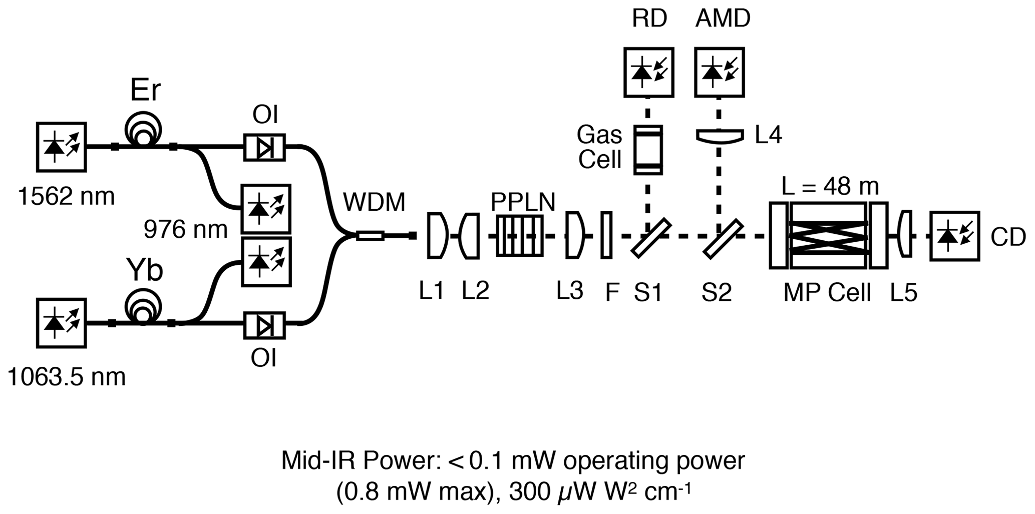
Figure 2Mid-IR source schematic. Er: erbium-doped fiber; Yb: ytterbium-doped fiber; OI: optical isolator; WDM: wavelength division multiplexer; L1-5: lens; PPLN: periodically poled lithium niobate; F: Ge filter; S1-2: beam splitter; MP cell: multi-pass cell; RD: reference detector; AMD: amplitude modulation detector; CD: cell detector.
Both the signal laser (1562 nm distributed feedback) and pump laser (1063.5 nm distributed Bragg reflector) are computer-controlled for wavelength scanning. The laser outputs are amplified in custom-built rare-earth-doped erbium (Er) and ytterbium (Yb) fiber amplifiers and produce up to 500 and 800 mW of optical output power. The fiber outputs are fusion-spliced to a wavelength division multiplexer (WDM). The fiber gain sections are backward-pumped by Bragg grating stabilized diode lasers (976 nm). Faraday optical isolators are used to minimize optical feedback to the seed lasers and fiber amplifier gain section. The combined fiber amplifier outputs are focused into a 1 mm thick and 50 mm long nonlinear periodically poled lithium niobate (PPLN) crystal to generate tunable mid-IR radiation. The signal (MFD=9.5 µm) and pump (MFD = 6.2 µm) beams are imaged (M=18) into the PPLN crystal with a two-lens system consisting of a f=2.75 mm aspheric lens (L1 in Fig. 2) followed by a plano-convex f=50 mm CaF2 lens (L2 in Fig. 2). The PPLN crystal is mounted to a copper block attached to a Peltier element and is heated to a temperature of about 40 ∘C to satisfy the phase-matching condition. To maximize the conversion process in the PPLN crystal, the polarization of the individual signal lasers is adjusted to a linear polarization state by in-line polarization controllers (not shown). As shown in Fig. 2, the converted mid-IR idler beam at the output of the PPLN is imaged by a CaF2 lens (L3, 50 mm) into the multi-pass absorption cell (MP) configured for an effective optical path length of 47.6 m. The remaining unconverted signal and pump radiation exiting the PPLN are removed by a germanium filter (F), and reflections off this filter are directed onto a series of absorbent glass filters (not shown). The PPLN module is shielded to prevent scattered pump and signal light from reaching the detectors in the detection module. The mid-IR beam then passes through two beam splitters (S1 and S2) before being directed into the MP. The first (S1) splits off ∼ 1 % of the beam, which is directed through a cell containing pure ethane (C2H6) (0.4 torr) and onto the reference detector (RD) for computer-controlled passive wavelength locking and/or tracking. The second beam splitter (S2) splits off 50 % of the remaining beam and is then focused by a 25 mm CaF2 lens onto an amplitude modulation detector (AMD). This allows close matching of the beam intensities and spectral features on the AMD and cell detector CD (L5, f = 25 mm CaF2 lens) to remove common-mode optical noise from the laser source assembly, including fiber-optic components. Neither apertures nor special coatings were applied in the detection module housing to suppress scattered light except for two beam dumps to reduce the impact of reflections originating from the immersion lens of each detector. The optical components are affixed to the baseplate by UV-cured epoxy after alignment.
2.2 MP cell and opto-mechanical design
Similar to the patented multi-pass cell design employed in CAMS-1 (Richter et al., 2015), the present MP offers a long path length (47.6 m, 49 round trips) and smaller sampling volume (∼ 1 L) than traditional Herriott cells. This is accomplished employing a sealed hollow-core tube in addition to an outer cylindrical tube that provides a vacuum-tight optical sampling cell. The inner tube is mounted centered to the cell's longitudinal optical axis, reducing the sampling volume between the two spherical mirrors of a traditional Herriott cell. Its diameter is limited to a radius that provides sufficient clearance of the recirculating beams between the two spherical mirrors. In addition, this patented design (Richter, 2013) significantly reduces the optical scattering that is received by the detectors (Richter et al., 2015). A solid non-flexing opto-mechanical coupling between the DFG components and the detectors is of utmost importance, as it minimizes intensity perturbations and optical baseline shape changes. One end of the multi-pass cell is mounted solid to this base assembly, while the other end is left floating to avoid mechanical stress due to thermal expansion when the system is not actively temperature-controlled (not in use).
The core inner tube of the MP cell is made out of carbon fiber, providing excellent stiffness and low thermal expansion. The MP cell spherical mirrors have an outer diameter of 63.5 mm with a centroid circular hole of 35 mm, prescribing a torus (donut) shape. The mirrors are mounted to a cylindrical flange, which in turn is suspended by five polished stainless-steel rods connected to the end of the inner tube flange. The opto-mechanical arrangement allows the flange to slide along the rods for adjustment of the mirror separation to allow adjustment for tolerances of the MP mirror radius of curvature and obtain a circular pattern with the desired path length and number of round-trip reflections. The mirror flange also accommodates a simple tip-and-tilt design to compensate for any machining tolerances of the mirrors or angular offsets of the carbon-fiber inner tube. A borosilicate glass tube is used as the outer cell body to provide visible access to trace an alignment beam. The beam is launched from one side of the MP cell and exits the cell on the opposing side, allowing for a compact setup with a close mounting of detectors. The entire spectrometer, including the MP cell, DFG laser source with seed lasers and fiber amplifiers, current and temperature controllers, FPGA, and power supplies, is arranged into a compact package that fits into a 30.5 cm diameter pressurized and thermally controlled enclosure. All optical fibers are embedded in memory foam to minimize the pickup of acoustic noise and prevent the movement of the optical fibers during airborne operation.
2.3 Electronics: power supplies, detectors, filters, preamps, FPGA, and communications
For this instrument, electronics and control systems were designed to support autonomous and calibration-free operation. This included the use of low-power-consumption electronic components, minimized thermal impact, and reduced weight and size. Electronic components and circuits were designed to operate with a low electronic noise floor well beyond desired sensitivity requirements. One method to achieve significant savings in weight and size was accomplished by replacing large and heavy linear power supplies with switching power supplies.
Desired electronic performance was achieved by employing (1) low-noise (Vpp<5 mV output) power supplies (PS) with appropriate filtering, (2) a judicious design of power and grounding pathways, (3) low-noise laser diode (LD) drive electronics and low-noise detector amplification, (4) all components controlled by a single embedded computer with synchronized arbitrary waveform generation and data acquisition at 320 kHz, and (5) computerized signal processing, yielding an electronic noise floor corresponding to a fractional minimum absorbance of Amin∼1– for a power level of ∼ 10–20 µW. All electronic components are schematically shown in Fig. 3, and further details regarding items (4) and (5) above will be discussed in Sect. 2.6.
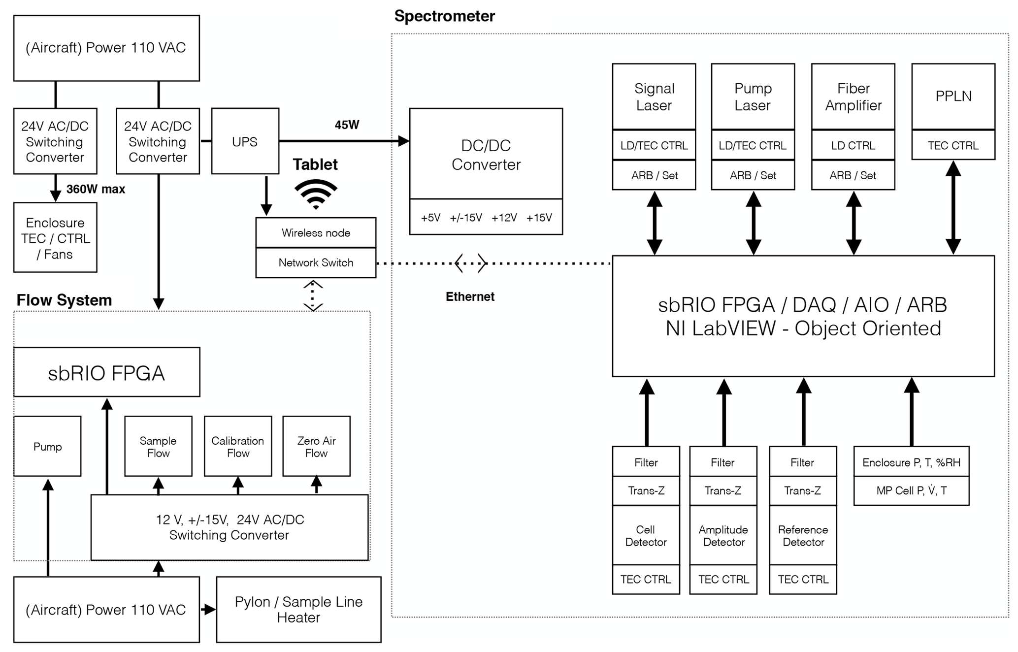
Figure 3Electronics and power schematic. UPS: uninterruptible power system; LD: laser diode; TEC: thermoelectric cooler; CTRL: controller; ARB: arbitrary waveform output; Set: set-point voltage output; DAQ: data acquisition; AIO: analog input–output; Trans-Z: trans-impedance amplifier; P: pressure; T: temperature; V: volumetric flow.
The CD, AMD, and RD detectors are three-stage Peltier-cooled (−60 ∘C) Vigo HgCdTe detectors (D*∼ 5×10¹⁰ at 1 kHz, Rs ∼ 500k, Cs ∼ 400 pF, d = 0.1 mm) with immersed ball lenses (d = 1 mm), providing almost identical response and noise characteristics. The detectors, operating in photovoltaic mode, are matched to low-noise trans-impedance amplifiers (TIAs) directly located at the detectors, yielding a trans-impedance gain of ∼ 100×103. The TIA outputs are sent into band-pass (BP) filter channels for each detector before digitization by the computer system. The CD TIA output is also sent into a low-pass (LP) filter channel to measure the transmission power of the laser through the MP cell, allowing for compensation of beam path fluctuations and mirror degradations. The spectrometer computer system is based on a real-time Linux host and a field-programmable gate array (FPGA) used for all input–output (IO) functions. The FPGA controls the arbitrary waveform generator and the 16 bit analog-to-digital (AI) converter as well as custom timing and safety control of the laser drivers. The FPGA also handles housekeeping (temperatures, pressures, flows, etc.) using a combination of AI, AO, DIO, and I2C sensors. Communication between the spectrometer, flow system (see Sect. 2.4), operator, and service technician is handled by a Wi-Fi router with a built-in cellular modem. The system real-time clock is set via a Network Time Protocol (NTP) time server onboard the aircraft. The operator controls the system using either an iPad or Android device. Figure 3 shows a schematic of the various electronics systems.
2.4 Calibration, flow, and pressure-stabilized optical enclosure systems
The gas handling system (Fig. 4) is comprised of (1) an inlet system with a port for introduction of zero air and calibration mixtures, (2) zero air and calibration cylinders with appropriate flow control (FC) and suck-back controllers, (3) the MP cell with inlet pressure control (PC) and outlet flowmeter (FM), (4) the vacuum pump with manual shutoff and flow control values (V1 and V2), and (5) a real-time Linux computer (not shown) with integrated FPGA (analog, digital, input–output).

Figure 4Flow system diagram. V1-2: flow control valve; V3-5: pressure relief valve; PC: pressure controller; FC: flow controller; FM: flowmeter; MPC: multi-pass cell; CAL: calibration gas cylinder; TEC AC: thermoelectric air conditioner; filter: 3 µm particle filter.
Ambient air is sampled perpendicular to the aircraft flow through a heated stainless-steel inlet (35 ∘C, 1 cm i.d.) located outside the fuselage boundary layer and is drawn through a heated teflon (PTFE) line, through a 3 µm particle filter, through a pressure controller (MKS640A), and into the MP. The total inlet length from the inlet entrance to the cell entrance is ∼ 6 m. The MP cell pressure is controlled to 73 torr ±0.1 torr. The reduced-pressure gas is fed through the pressure-stabilized vessel surrounding the entire optical system (shown in Fig. 1 as the cylinder) and into the multi-pass cell using flexible Teflon tubing to reduce vibration coupling. Similarly, all electrical connections to and from the optical system were directed through vacuum feedthroughs. For a typical sample flow rate of 4 slm we achieve a cell residence time of ∼ 1 s (1∕e). The inlet ∕ sampling cell time lag, which varies with altitude, ranges between 2.5 s (25 kft.) and 5 s (at the surface), and all final data have been appropriately time-shifted to account for this.
The flow system computer controls all functionality (flows, pressures, temperatures) and sequencing of the flow system in accordance with commands from the spectrometer computer system. The system operates in three modes: ambient, background, and calibration standard. In the ambient mode, outside ambient air is drawn through the multi-pass cell for 5–7 min after which the background mode is engaged. Here ultrapure air (Scott Marrin) from the air cylinder is fed to the inlet tip at a higher flow rate than the cell intake flow, thereby excluding ambient air from the system and allowing instrument backgrounds to be recorded. In total, zero air is directed into the inlet for 90 s, which includes 30 s of background acquisitions and 30 s delay times before and after each background to allow sufficient time for flushing and system stabilization. After ∼ 90 s, the ambient mode is engaged again and the cycle starts over. During the calibration standard mode, a known mixing ratio of C2H6 to CH4 (20 ∕ 2000 ppbv) is fed into the zero airstream by a flow controller, which is then added to the inlet. This was performed before and after each flight to verify instrument accuracy. During ambient and background modes, a small suck-back flow (0.3 slm) is engaged to draw away any residual standard trapped in the addition line.
Acquisition of zero air backgrounds throughout each flight not only chemically zeros the entire gas handling flow path, which is important for elimination of outgassing effects after high-transient-concentration sampling, but also removes nonzero retrieved ethane mixing ratios due to optical effects. This frequent zeroing further allows us to assess instrument precisions throughout each flight by fitting the zero air background spectra during each zeroing period. In comparison to previous systems, the flow system here is made less complex by replacing heated scrubber systems and more complicated calibration systems with zero air and calibration gas cylinders as well as simplified gas handling paths. By controlling the air and standard gas flow rates, known concentrations can be generated and are used to verify the instrument accuracy and precision.
As shown in Fig. 1, the optical enclosure is thermally insulated, while the temperature of the entire optical train is controlled. In an effort to simplify and reduce costs, the pressure vessel (enclosure) was designed from a stock 30.5 cm o.d. 6061-T6 aluminum pipe. The walls were turned down with a lathe in equidistant sections along its longitudinal axis, leaving thicker sections in the middle and end to accommodate the mounting of end plates and rack mounting points. The internal spectrometer assembly was suspended via vibration isolators to the outer shell, while the vessel was mounted to the rack with wire rope shock isolators. One end plate was used for easy access to the DFG module, while the opposing end was used to feed through the gas and electrical connections and serve as a mounting plate for the air conditioner. However, during the first two field campaigns in the summer of 2016 and the winter 2017, the sealing area on the vessel end surfaces was poor, resulting in a higher leak rate. This was subsequently rectified by increasing the sealing surface on both end plates by replacing an O-ring with a flat 10 mm wide rubber gasket. This significantly reduced enclosure pressure changes from values as high as 41 torr when the B200 cabin pressure changed by 144 torr as the aircraft ascended from 0.5 to 9.1 km over the course of 12 min during the summer 2016 campaign to values as low as 0.3 torr change in the enclosure when the cabin pressure changed by 19 torr during an ascent from 0.5 to 4.5 km during the fall 2017 campaign. Sometimes rapid cabin pressure changes occurred about 1 min or less prior to the aircraft changing altitude. Since such cabin pressure changes can occur over time periods much faster than can be captured by frequent zeroing and/or calibration, optical enclosure pressure stabilization is required for robust high performance. The poor pressure stabilization during the summer 2016 campaign provided us with a direct quantitative figure of merit in terms of pressure change per unit time that must be achieved for high performance. During flight, enclosure pressures are maintained around 615 torr by pumping on the enclosure while employing an MKS 640A pressure controller and adding a small controlled flow (∼ 0.2 slm) of zero air into the enclosure.
2.5 Air-conditioning and uninterruptible power system
The air-conditioning system was designed to minimize size and complexity and consists of two (Qmax = 341 W each) thermoelectric cooler (TEC) elements attached to one end plate of the enclosure and adjacent fans attached to the inside enclosure wall to circulate the air. The enclosure internal temperature was set to operate at 26 ∘C ±0.5 ∘C for a cabin temperature range of 10–30 ∘C. Compared to previous system designs, this is less complex but has a large power consumption and degradation in cooling efficiency when the difference between enclosure and cabin temperatures reaches >10 ∘C. The system warm-up time is 60–90 min from a cold start depending on ambient temperature and is mainly dependent on the instrument thermal mass reaching operating temperature. Attached to the optical enclosure is thermal insulating foam (thermal conductivity 0.035 W per (m*K)). The UPS system keeps all system components running for a minimum of 30 min except the air-conditioning and flow system during power switch overs from ground to aircraft power and during refueling. However, not keeping enclosure temperature–pressure constant during no-power aircraft operations requires 20–30 min for the instrument to restabilize in some cases.
2.6 Signal processing and software
This section provides an overview of the various software processing modules, and more detailed information will be presented in subsequent sections. The computer software is based on object-oriented LabVIEW and uses standard and custom plug-in software modules with the National Instruments Distributed Control and Automation Framework (DCAF) as well as custom FPGA code. To suppress asynchronous noise, the arbitrary waveform generator and data acquisition boards are controlled and phase-locked by the FPGA. An 800 Hz sawtooth waveform with a smooth recovery function drives the laser scan current. After averaging the CD, AMD, and RD signals onboard the FPGA to the desired time resolution, these signals are sent to the host for processing in the following steps.
-
Common-mode noise is mathematically removed for every measurement update by subtracting the AMD signal from the CD signal using the expression CD-R*AMD, where R is calculated as the ratio between the CD and AMD scan amplitudes. This provides a mathematical balancing of the CD and AMD powers.
-
The CD-R*AMD signal is wavelength-locked by sub-channel-shifting the recorded CD-R*AMD spectra using the C2H6 high-concentration cell in the RD path as a reference. Here we utilize a manifold of at least 30 individual strong ethane vibrational–rotational lines spanning a 0.2 cm−1 range centered at ∼ 2996.8 cm−1, which are the same lines employed by Yacovitch et al. (2014). This simplified approach was found to be sufficient compared to the CAMS-1 instrument, whereby the laser current is used to actively stabilize the wavelength in a feedback loop.
-
Residual instrument noise is removed by periodically recording and subtracting the instrument spectral background by introducing ultrapure air into the multi-pass cell for a period of 90 s and repeated every 5 to 7 min before a new background is acquired, as previously discussed. This yields an ambient duty cycle ranging between 83 % and 88 %.
-
To retrieve the measured concentration, Sect. 2.7 discusses further details of the fitting procedures employed in determining ambient ethane concentrations using background-subtracted spectra and measurements of cell pressure, temperature, and path length along with spectroscopic parameters from the infrared database provided by Harrison et al. (2010) using the Beer–Lambert absorption law.
The software fits multiple absorption features in the same scan window and interference deconvolution. Figure 5 shows an example of fitting out multiple species (C2H6, CH4) in the same scan, but in this case the CH4 line strength only yields measurement precisions of ∼ 30–40 ppbv, as the priority for scan window selection was to obtain maximum precision of C2H6. The DFG-based system has a wide and flexible tuning range, and judicial selection of the wavelength region can accommodate multiple species to fit different measurement requirements. All measurement and housekeeping data as well as unprocessed (raw) CD, AMD, and RD spectra are stored on a local USB–SD drive that can be accessed via a router by either Wi-Fi or LAN connections.
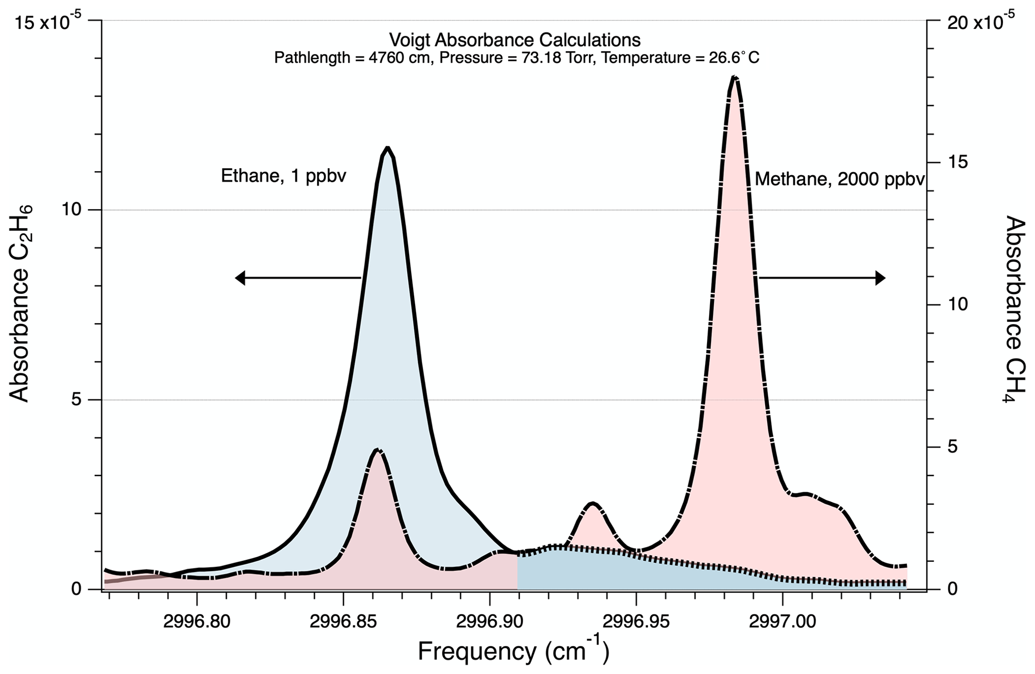
Figure 5Ethane and methane simulated lines using Harrison et al. (2010) and HITRAN 2016 line parameters. Note the rather large wavelength spread of the ethane background data caused by a multitude of small ethane and methane lines in the wings. In the text we refer to this as a pedestal, and it is further highlighted by the blue area at the high-frequency side of the ethane absorption wing.
A major effort was devoted to operating the instrument autonomously during flight, allowing the instrument, depending on the “instrument state”, to take preprogrammed actions such as pause, restart, safe state, or shutdown of individual tasks and/or software modules or the complete instrument if needed. All actions and error messages are logged to help trace potential issues later. At power-up, the instrument runs a series of “checks” and if passed enters “ambient” measurement mode without the need to “calibrate” as the measurement is based on the first-principle Beer–Lambert absorption law.
2.7 Direct absorption spectroscopy
Figure 5 shows a simulation of the resulting absorption spectrum for 1 ppbv of ethane employing typical conditions of temperature (26.6 ∘C), pressure (73.2 torr), and a path length of 4760 cm using Voigt line profiles and the Harrison et al. (2010) database for ethane. As discussed by Yacovitch et al. (2014), the HITRAN database for ethane does not satisfactorily reproduce the ethane spectrum in the 3 µm region, and this was further verified by our comparisons of the direct absorption results with independently calibrated standards. We also show the spectrum for 2 ppmv of methane using the 2016 HITRAN database. This simulation closely approximates the scan wavelength range used during the ACT-America studies. As can be seen, methane introduces a positive interference on ethane. At the ethane line center, these simulations indicate that 2 ppmv of methane produces an error of + 347 pptv on ethane. This is in close agreement with laboratory results employing calibrated methane standards. Such measurements reveal that 2 ppmv of methane results in an error of + 342 pptv on the retrieved ethane. Although we can remove this interference using the methane line at 2997 cm−1, we instead employ the more precise onboard measurements of methane from a PICARRO G2401 m calibrated in-flight with standards traceable to the WMO X2014 scale (ORNL dataset reference). Once the data have been carefully time-shifted to match ambient features, this is accomplished by subtracting the PICARRO methane values multiplied by the 342 pptv ∕ 2000 ppbv factor from our retrieved initial ethane values. Future instrument configurations will employ the 2997 cm−1 absorption line and stronger CH4 features to remove this interference without the dependence on another instrument.
A key requirement for maintenance-free operation is the implementation of absolute first-principle direct absorption measurements via the Beer–Lambert absorption law:
Here, I and Io are the transmitted and incident intensities, respectively, acquired from measurements of the CD at each wavelength step, σ is the absorption cross section, L is the absorption path length, C is the mixing ratio of ethane, N is the air number density flowing in the absorption path at the sampling temperature and pressure, and A is the resulting absorbance (base e). Prior to each ambient acquisition, background spectra (CD-R*AMD)Bkg are acquired by directing zero air into the inlet. The background spectra are averaged and used to subtract from the subsequent ambient acquisitions to obtain a relatively flat transmission spectrum. The remaining baseline curvature is removed using a third- to fifth-order polynomial function. Io values are determined on the CD signal at each wavelength step using a low-pass filter to remove the absorption feature. The high-pass filtering of (CD-R*AMD) provides measurements of the differential absorption spectrum as dI values at each wavelength step. We then calculate an absorbance at each step from
Employing the Marquardt–Levenberg nonlinear fitting algorithm (Marquardt, 1963; Levenberg, 1944) with these absorbance measurements along with spectral parameters from Harrison et al. (2010) for ethane and from the 2016 HITRAN database for methane and water, Voigt line shapes, and measurements of pressure, temperature, and path length, we calculate the best-fit absorbance profile. The system software supports fitting the integrated area of each spectral feature employing the appropriate integrated absorption cross sections in determining mixing ratios via Eq. (2). However, it was found that fitting to a peak absorbance using the line-center absorption cross section was less susceptible to baseline noise, particularly from optical fringes, and slow changes in baseline curvature. This latter approach was therefore used throughout the campaigns in retrieving ethane mixing ratios. In this approach, a peak ethane absorption cross section was determined at a line-center σ(ν0) of cm2 molec.−1 from the Voigt simulations shown in Fig. 5 employing the Harrison et al. (2010) database for the 2996.85 cm−1 manifold of ethane lines after accounting for the relatively broad-absorption baseline pedestal shown. Figure 6 shows raw and fitted spectra acquired for ethane (4.23 ppbv) and methane in our laboratory. The methane feature underlying the ethane is still present but is not visible here since the methane almost perfectly overlaps with ethane. Since the width of this fit is not optimized for the methane feature on the right, its absorbance is underestimated.
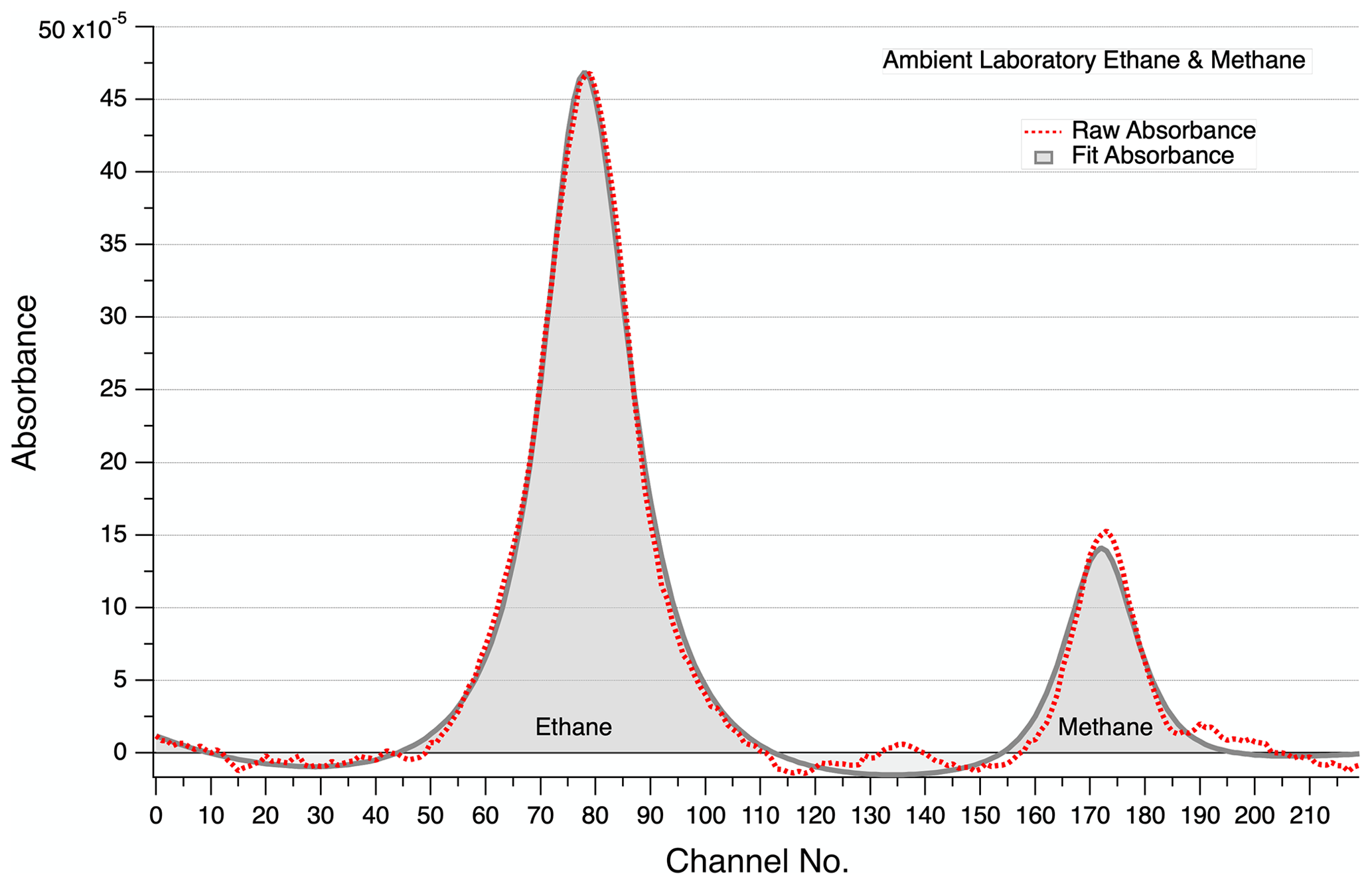
Figure 6Ambient ethane and methane raw and fit spectra acquired by sampling laboratory air. The spectra are in channel numbers. The fit indicates an ethane mixing ratio of 4.23±0.025 ppbv, while the methane corresponds to 1591±30 ppbv. The methane feature underlying the ethane feature shown in the previous figure is still present but not evident in the fits here since this feature almost perfectly overlaps with ethane. The methane feature on the right in this scan is clearly underestimated since we have not optimized the width of this feature. The very weak methane feature between ethane and methane also shows up on the raw spectra but is not properly fit here.
The overall cross section uncertainty quoted by Harrison et al. (2010) is ±6 % (1σ), after considering a correction factor applied to their data to match results from Pacific Northwest National Laboratory (PNNL) measurements. Since that study determines the results at various pressures, including those around 76 torr, we assume that the uncertainty in the exact individual line positions is taken into account. This is important since our recorded ethane feature is the convolution of at least 30 individual lines at our 73 torr sampling pressure, and small line position errors could add to the uncertainty of our deduced peak line-center absorption cross section above.
As indicated, known calibration mixtures of ethane–methane diluted in zero air from a set of working Scott Marrin standards were introduced into the inlet (20 and 2000 ppbv) before and after each flight to further validate the direct absorption retrieved values and the fitting approach implemented. Typically, the retrieved ethane values for the working standards were lower than the expected input values based on the manufacturer-assigned values times the measured dilution ratio. All reported ambient ethane data were thus based on direct absorption values corrected by the daily working standard correction factors (assigned cylinder mixing ratio of retrieved values during preflight and postflight calibrations). Since this procedure relied upon the accuracy of the Scott Marrin working standards, we also verified these standards in the laboratory based on multiple direct absorption measurements employing the CAMS-1 and CAMS-2 instruments. In addition, prior to the fifth field deployment we measured the mixing ratios of various additional ethane standards by direct absorption. These standards included (1) a gravimetrically prepared ethane–air standard (nominal 5 ppmv) from Apel-Riemer Environmental, which in turn was evaluated by Riemer against NIST Standard Reference Material (SRM) gases, and (2) two additional ethane standards in the 0.3 and 3 ppbv range employing Niwot Ridge air prepared and analyzed by the NOAA/ESRL Global Monitoring Division and subsequently analyzed by Detlev Helmig's Atmospheric Research Laboratory at the University of Colorado Institute of Arctic and Alpine Research using standards tied to the Global Greenhouse Gas Reference Network (see for example Helmig et al., 2016). The latter two standards were measured in our laboratory by direct absorption without dilution. Collectively, all the ethane standard comparisons resulted in agreement between our direct absorption values and the assigned cylinder values in the range between −1.2 % and + 4.8 %. It is important to note that the NOAA standards were used by Baier et al. (2019) in their programmable flask package (PFP) ethane measurements. Figure 9a shows an orthogonal distance linear regression (ODR) plot of our direct absorption results (with the daily corrections applied) integrated over the PFP time base as a function of the PFP ethane results for the entire spring 2018 fourth deployment. Additional ambient ethane ODR comparisons for the second through the fourth field campaigns are provided in Table 2, and these results show agreement between CAMS and the PFP to within 3 %. Collectively, all ethane comparisons (ambient and cylinder standard measurements) show agreement within the ±6 % (1σ) Harrison et al. (2010) cross section uncertainty value.
Table 1Total measurement uncertainty estimates (TMUs) during all ambient ethane measurements >0.5 ppbv acquired during three of the field campaigns.
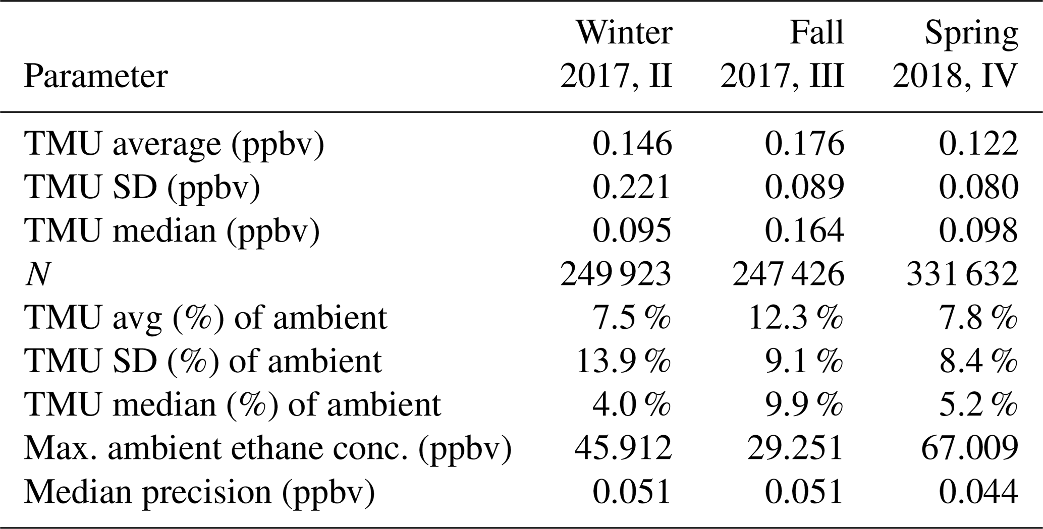
Table 2Orthogonal linear regressions of the fast CAMS data averaged over the PFP time base vs. the PFP data for three of the field deployment phases.

2.8 Background acquisitions, diagnostics, and data handling
This section will discuss additional sources of uncertainty associated with background changes measured during zero air background additions. Backgrounds are acquired by overflowing the inlet with zero air every 5 to 7 min using ultrapure compressed air. Initially, a 5 min ambient period was chosen before a new background was acquired. Numerous instrument improvements during each field deployment phase enabled zero air background subtraction to be extended to 7 min by the fourth campaign in the spring of 2018. These backgrounds not only provide a semicontinuous assessment of the instrument measurement precision, but also represent an important component of the measurement accuracy. In contrast to many other studies that report a single precision and accuracy assessment for an entire study, we report the measurement performance with every ambient cycle, and over the course of each mission these assessments cover the full range of aircraft maneuvers of pitch, roll, aircraft ascents and descents, cabin pressure and temperature changes, and vibrations. The resulting data, reported as histograms, thus provide a more representative picture of the true instrument performance.
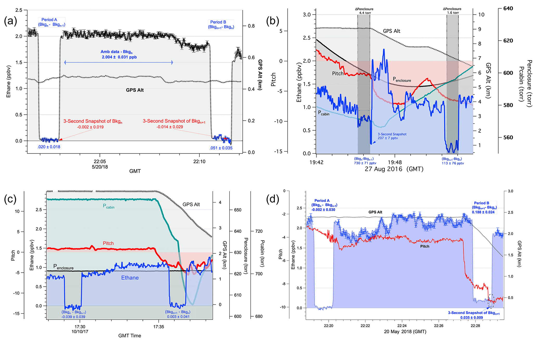
Figure 7(a) Pre- and post-ambient background acquisitions during the fourth field deployment phase. The background values have the same units as the ambient ethane structure (ppbv). The dark blue circles represent the derived mixing ratios of the background difference (present – previous). The dark blue line highlighted by the numbers in red represents a 3 s snapshot of the new background itself. The enclosure pressure change (not shown) over the entire time period here is 0.36 torr. This deployment phase represents the latest improvements whereby the cell and input–output optics have been further stabilized (see text). (b) Pre- and post-ambient background acquisitions during the first field deployment phase on 27 August 2016 before the enclosure was sealed. The blue traces in the shaded regions show background acquisitions before and after the ambient acquisitions. In this case the leaking enclosure caused a pressure change of 4.4 torr in the first background region as the cabin pressure changed, causing very dramatic changes not only in the fast noise but also a shift in the background of 0.523 ppbv in this case between the (Bkgn – Bkgn−1) and the 3 s snapshot. (c) Pre- and post-ambient background acquisitions during the third field deployment phase in the fall of 2017 in the same format as Fig. 7a. As the cabin pressure changes by 37 torr on the descent during the second background period, the enclosure pressure is stable to within 0.23 torr. The optics have not been stabilized here, so changes in pitch have a more dramatic effect on the background structure. (d) Pre- and post-ambient background acquisitions during the fourth field deployment phase. During background Period B the aircraft pitch changes, causing a small optical change in the background structure, which in turn changes the background fit value by ∼ 0.153 ppbv.
Figure 7a shows two background (Bkgn, Bkgn+1) acquisition periods during the fourth deployment phase during the spring of 2018. The first background (Period A) is prior to the ambient period, and the second one is after the ambient period (Period B). The entire 90 s background periods, which includes 30 s for background acquisition plus the two flushing periods, are shown. Each of the ambient-derived mixing ratios shown here employed Bkgn acquired during Period A to subtract, and thus as a means to remove, the optical background structure. The backgrounds are fitted and treated with a procedure identical to the ambient acquisitions that uses the previous background to subtract and remove residual optical noise. In the case of Period A, we show the derived mixing ratio results from the residual fit of Bkgn acquired during this period minus Bkgn−1, acquired 7 min prior (not shown). As illustrated, the fit of the resulting background difference (Bkgn – Bkgn−1) yields a stable background difference (0.020±0.018 ppbv) close to zero. The instrument precision (1σ) was determined for each associated ambient period from the mixing ratio standard deviation of this background fit difference. We assign a single precision for each ambient period, and these are plotted as error bars with each 1 s ambient result. This standard deviation is close to that determined for the ambient acquisition period indicated (±0.031 ppbv) and further supports our precision estimates. As true ambient variability cannot be ruled out, the larger ambient imprecision compared to the background fit difference is not surprising. This result, among others and laboratory measurements, shows that the precision is concentration-independent. During the last 3 s of each background cycle before valve switching back to ambient, we plot a 3 s snapshot of ultrapure air (background), whereby we subtract the background acquired during the past 30 s from this 3 s snapshot as a means to highlight fast changes in the present background. This background difference is annotated in red. Under perfectly stable conditions, one should expect values around zero without significant background drifts over the course of the 30 s. As discussed previously, the new background (Bkgn in this case acquired over the full 30 s) is then used for the subsequent ambient spectra. We emphasize here that the 3 s snapshot period is a diagnostic meant to show fast background changes relative to the full 30 s new backgrounds that are employed for the next ambient period. During Period B, we show a plot of the newest background minus the previous background (Bkgn+1–Bkgn). This results in a value of 0.051±0.035 ppbv and a snapshot value of ppbv.
During stable instrument performance, as indicated in Fig. 7a, not only should the 3 s snapshot values lie around zero within the indicated precision, but the background differences before and after each ambient should also be equivalent within the measurement precisions. In this case the background during Period A (Bkgn–Bkg ppbv) is equivalent to the background during Period B (Bkgn+1–Bkgn = 0.051±0.035 ppbv). However, perturbations from the various sources mentioned above during flight will show offsets not only between adjacent background differences, but also between the latest background and the 3 s snapshot values. Figure 7b exhibits such extreme behavior during the first field deployment phase before the enclosure was pressure sealed. The snapshot value of 0.207±0.007 ppbv during the 3 s period (shown by the notch) not only yields a value far removed from zero, resulting from the enclosure 4.4 torr pressure drift, but also a background change of 0.523 ppbv. The second background period, furthermore, revealed an additional background change from the 0.207 ppbv value to 0.113 ppbv. As a result, our ethane data from the first deployment phase conducted during the summer of 2016 are degraded by pressure changes in the optical enclosure and not included in our final reported ACT data. However, this figure and the resultant data show the magnitude that pressure changes in the optical enclosure can exert on the retrieved ambient ethane data and hence the importance of pressure control. Figure 7c shows the background behavior during the third deployment phase in the fall of 2017 that is typically observed once the temperature of the system has been restabilized for at least 30 min after takeoff and after the enclosure pressurization problem was fixed. As can be seen, large fluctuations in cabin pressure no longer affect the enclosure pressure and hence the background structure.
Although the background profiles, and hence the quality of the ambient ethane data, were significantly improved during the fourth field deployment phase, as shown in Fig. 7a, we still observed moderate background shifts even after system temperature stabilization. Figure 7d, which was acquired on the same day as Fig. 7a, provides one such example. The background data during Period A reveal essentially the same excellent performance as Fig. 7a. However, the background data in Period B reveal a residual system sensitivity to what we believe are rapid changes in aircraft pitch as the aircraft was preparing for landing, but these have been observed during other occasions even after improved optics stabilization. Although the precisions are still excellent, here the background jumps from an average value of −0.002 to 0.188 ppbv, and the 3 s snapshot period previously unobservable becomes immediately evident during the second change in aircraft pitch in Period B. To account for such additional time background changes we applied an additional correction to the final ambient ethane data. Referring to Fig. 7d, we linearly interpolate the background data between a zero concentration at the end of Period A (which represents the new background that is applied to the subsequent ambient data) and the average background data at the start of Period B. This linear background temporal interpolation, which is subtracted from the ambient data between the two background periods, accounts for linear background drifts. Obviously, nonlinear drifts or jumps in the true background will cause data errors. Our subsequent data analysis using our ethane data flags such time periods, especially where there are large background changes and/or the ethane data show such an artificial time dependence. Flagged time periods are manually examined for validity. Using this same logic for the next ambient period, we interpolate between 0 ppbv (Period B) to the mean background at the start of the next background period (0.038±0.032 ppbv). We estimate the component of uncertainty due to such background changes over each ambient time period by 1∕2 of the mean value at the beginning of the next background period. Section 3.1 further discusses the various components of our estimated total measurement uncertainties.
CAMS-2 was designed to realize a small, lightweight, fully autonomous, and calibration-free instrument. While several aspects of the CAMS-1 design were inherited by CAMS-2, a number of new approaches were implemented for CAMS-2 and continually evolved for the entire duration of the field deployments. Improvements and simplifications between the CAMS-2 and CAMS-1 designs will be compared at the end of this section.
3.1 Improvements with each field deployment phase
The most impactful improvements were implemented before the third and fourth field deployment phases. Prior to the third field deployment phase, the enclosure pressure was stabilized and, in addition, the optimum PPLN phase-matching temperature was de-tuned to reduce a small halo spatial emission mode exiting the PPLN crystal. Although this substantially reduced mid-IR power, it significantly improved the matching between the CD and AMD arms, resulting in improved performance, as will be further discussed below in this section. Prior to the fourth field deployment phase in the spring of 2018, we further addressed the mechanical stability of various optical components.
The mechanical construction between the MP cell and the launching optics was improved by stabilizing bars, reducing movements induced by accelerations. An improvement of ∼ 2× in baseline concentration stability was verified by inducing instrument tip-and-tilt actions in the lab. The mechanical stability is not only affected by accelerations, but also by enclosure temperature variations that reached ±0.5 ∘C over 5 min during normal flight operations. Two potential causes were identified: (1) lack of efficient air exchange between the thermoelectric cooling unit and optical components and (2) low thermoelectric efficiency at >30 ∘C cabin temperatures. This is in contrast to CAMS-1 temperature control of ±0.1 ∘C and is a contributor to performance degradation in non-laboratory environmental conditions. This furthermore necessitated at least 30 min of restabilization before optimal performance was achieved after takeoff. Even though the temperature changes are relatively slow, they can affect the mechanical stability through thermal expansion but also alter the optical properties of active and passive fibers, as well as perturb the nonlinear optical frequency generation process in the PPLN crystal. These components have previously been determined to be sensitive to temperature variations affecting short- and long-term drifts in the spectroscopic baseline (Weibring et al., 2006, 2007). Therefore, the PPLN compartment was insulated and the fiber trays were padded by foam, similar to CAMS-1, to insulate and slow down temperature variations as well as dampen fiber vibrations during airborne operation. This significantly reduced high-frequency noise.
Small PPLN temperature instabilities can result in secondary effects that alter the temporal and spatial beam propagation of the highly focused beams through the PPLN. According to Zhou et al. (2014), non-collinear focusing of the two beams into the PPLN crystal results in spatial deviation of the PPLN output from a Gaussian beam to a Gaussian beam with a donut-shaped halo component. The spatial evolution for propagation of such a beam deviates between the near and far field compared to the ideal Gaussian beam, making it especially difficult to record and remove common-mode noise with our subtraction approach, which is dependent on the fact that the spatial beam properties between CD and AMD detectors are only influenced by the cell transmission and not a spatial mismatch between the CD and AMD detector areas. This was confirmed to be present in CAMS-2 using a mid-infrared camera, while CAMS-1 did not show the same behavior. CAMS-1 and CAMS-2 use different focusing geometries, resulting in a more non-collinear phase matching in the latter case. Adjustments within the CAMS-2 design to attain minimal non-collinear phase matching could not be achieved. Therefore, CAMS-2 required temperature de-tuning of the PPLN crystal from the optimal-power-generating phase-matching temperature to suppress residual non-collinear phase matching, improving the spatial beam shape and degree of matching in the CD and AMD arms. The drawback of operating on the edge of the phase-matching bandwidth resulted in larger power instability induced by small ambient temperature perturbations.
The resulting low DFG power of 10–20 µW placed stringent requirements on the electrical noise of the system to ensure that the system is operating in the shot noise regime. New low-noise switching power supplies and filtering dedicated for the detector preamplifiers and sequential noise filtering were applied (see Sect. 2.3). A low-noise Vigo HgCdTe (MCT) detector type with a high shunt resistance was selected. The small detector surface area was mitigated by an attached half-ball immersion lens, making the apparent detector area 1 mm in diameter and allowing less demanding focusing conditions. The drawback of using a detector with a ball lens is that regardless of the incoming beam angle there will always be a reflection going straight back into the incoming beam (cat-eye effect), potentially causing optical feedback and associated fringing. While DFG is immune to direct feedback, mid-IR laser sources such as quantum cascade lasers are known to be affected by optical feedback. However, reflected and/or scattered beams in the present optical system can still produce optical fringe noise between enclosure walls and various optical components. To minimize such effects, optical components were tilted and reflected beams removed by beam stops.
The various performance-inhibiting thermal issues were mitigated before the fourth field deployment phase and resulted in robust high performance during airborne operations. The results can immediately be seen using histograms by comparing the precisions determined from the background measurements during the third field deployment phase in the fall of 2017 in Fig. 8a with those in Fig. 8b acquired during the fourth field deployment phase in the spring of 2018.
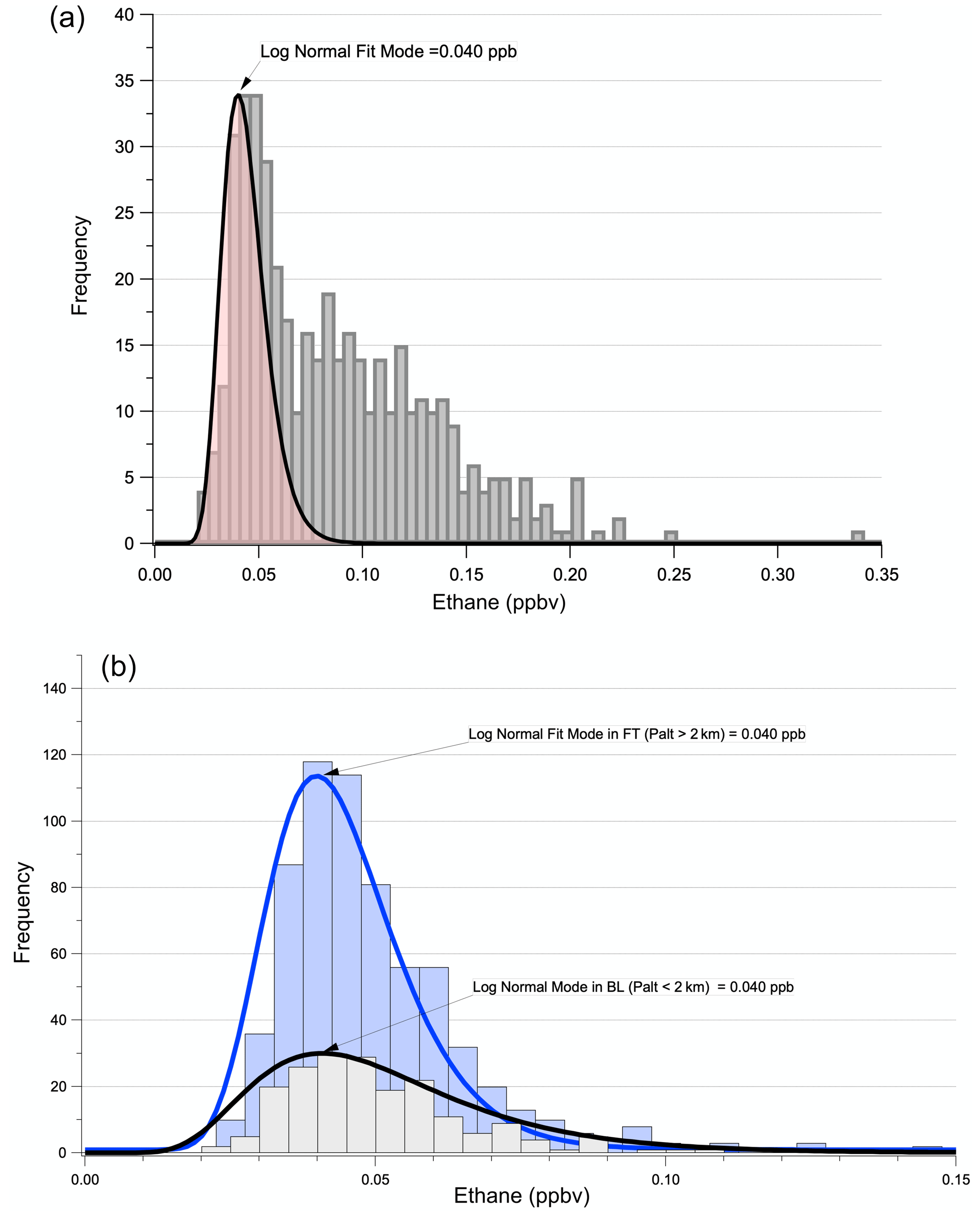
Figure 8(a) Precision histogram of all zero background measurements for the third field deployment phase (3–16 October 2017); bin width: 0.005 ppbv. (b) Precision histograms of zero air background measurements in the PBL and in FT acquired during the spring 2018 fourth field deployment phase using a bin width of 0.005 ppbv.
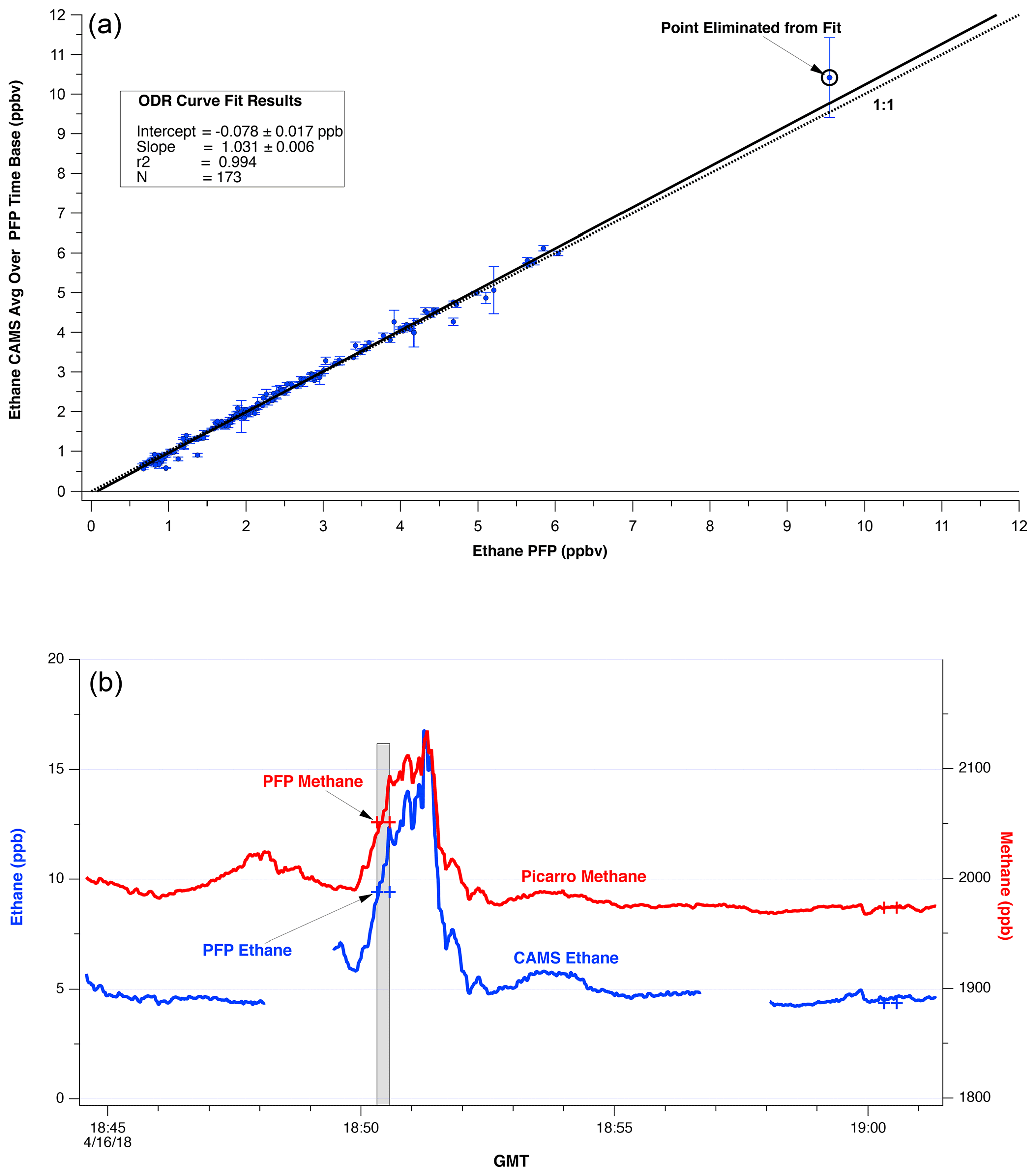
Figure 9(a) Spring 2018 IV field deployment phase final comparisons of CAMS average on PFP time base vs. PFP. (b) Temporal profile of ethane from the CAMS (blue lines) and PFP (blue crosses) measurements as well as PICARRO methane (red line) and PFP (red crosses) measurements. The gray shaded region shows the highly variable ambient results for the point eliminated in Fig. 9a.
We show in these figures histograms of the resulting 1 s background precisions acquired with each ambient acquisition period for the entire third and fourth field deployment phases, and the resulting lognormal fits and associated mode of the fits reveal both instantaneous noise and instrument drift since last background recording. In Fig. 8a, even though the mode of the lognormal fit reveals an excellent precision of 0.040 ppbv during the third field deployment phase, one can immediately observe a second distribution mode by the rather large tail in the histograms out to values as high as 0.340 ppbv. By comparison, the two histograms shown in Fig. 8b (one in the PBL with pressure altitudes <2 km and one in calmer, less turbulent free troposphere air at altitudes >2 km) both reveal only single mode distributions with lognormal-mode fit values of 0.040 ppbv throughout the entire fourth campaign and hence more stable instrument performance. One also observes a considerable number of background values in the 0.030 to 0.040 ppbv range. It is important to note that these comparisons, which reveal the effectiveness of our improvements, were acquired over all the various aircraft perturbations during both field deployment phases (i.e., pitch, roll, yaw, cabin pressure and temperature changes, and vibrations), which presented challenges for our ethane measurements. Showing precision histograms under all such conditions, particularly in both the turbulent boundary layer and the calmer free troposphere, further accentuates the dynamic nature of airborne performance and reinforces the fact that a single performance estimate does not truly capture this dynamic performance.
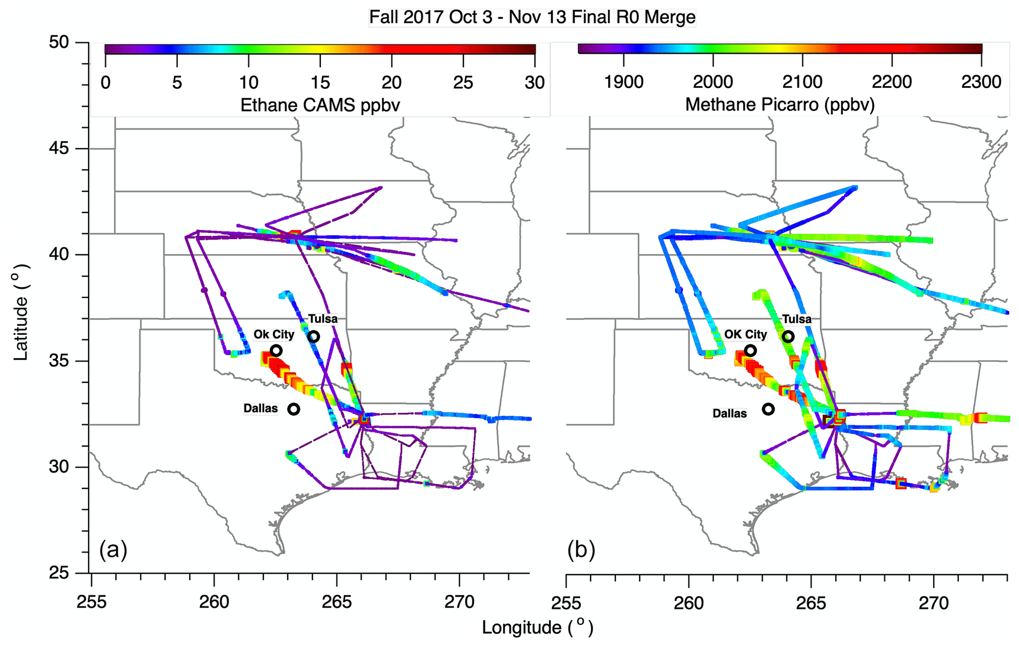
Figure 10Simultaneous ethane (a) and methane (b) over the southeast. The ethane measurements are from the CAMS-2 instrument, while methane measurements were acquired from a PICARRO instrument onboard the B200 aircraft.
As previously stated, the measurement precisions only reveal part of the performance story as changes in background structure acquired during zeroing between ambient acquisitions dictate the overall total measurement uncertainty (TMU). The TMU at the 1−σ level is comprised of five terms:
These terms are (A) the background precisions prior to each ambient acquisition period, (B) temporal changes in the background differences over the course of each ambient acquisition, as discussed in the previous section, (C) the uncertainty in the methane interference correction (0.342 ppbv ∕ 2000 ppbv [CH4±0.006]) as determined in the laboratory, (D) the PICARRO methane measurement error (±1 ppbv ×0.342 ∕ 2000 ppbv; https://doi.org/10.3334/ORNLDAAC/1556), and (E) the uncertainty in the fitting correction factor employing the input calibration standards. Table 1 shows the estimated TMU for three of the field deployment phases estimated during all the ambient measurements for ethane values >0.5 ppbv. The TMUs are given both in absolute ethane mixing ratios and the percent of the ambient values. The temporal changes in the background differences comprise the largest contribution to these TMUs. As can be seen, the median precisions are all less than 54 % of the TMU values, which for the latter values fall within the 0.095 to 0.164 ppbv range (4 % to ∼ 10 % of the ambient values).
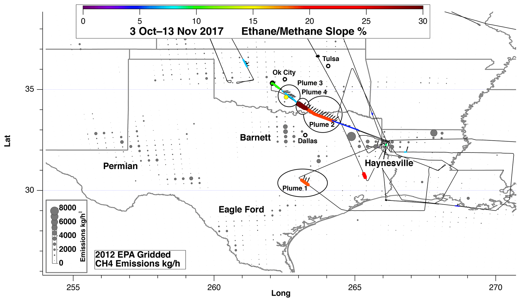
Figure 11Ethane–methane slopes over the southeast during the October–November 2017 time period showing three plumes with high ethane–methane slopes. The wind directions along the flight tracks are indicated by arrows (the wind speeds, WNS, are multiplied by 3 for emphasis). The four major shale plays in this region are indicated along with the 2012 EPA gridded methane emission rates in the gray-filled circles, which are sized by their emission rates.
Although the TMUs are quite good, they can be improved significantly by further mechanical stabilization of the optics towards aircraft pitch changes and improved temperature control of the optics within the enclosure, as well as optimized PPLN focusing geometry. As with our dynamic precision estimates, these dynamic TMU estimates truly reveal the instrument performance over the full range of aircraft maneuvers. The comparisons of the CAMS ethane measurements with the flask package (PFP) measurements acquired by NOAA on the same aircraft (Baier et al., 2019), discussed in Sect. 3.3, further support the lower range of our TMU estimates. In two of the three field deployment phases the median TMU as a percent of ambient values falls in the 4 % to 5.2 % range, which, as will be seen in Sect. 3.3, yields CAMS ethane values that are nearly identical to the PFP values to within 3 % ± 0.5 %. This also includes the third field deployment phase wherein the TMU estimate yields a median value of 9.9 %. Perhaps our TMU estimates in some cases overestimate the background drift component of uncertainty.
3.2 Comparison of CAMS-2 to CAMS-1 performance
In this section we compare the CAMS-2 ethane airborne performance from the fourth field deployment phase with that from airborne CAMS-1 ethane measurements employing a much heavier, larger, and more complex airborne system. CAMS-1 employs 2-f harmonic detection, while CAMS-2 employs direct absorption spectroscopy. Direct absorption spectroscopy has the advantage of yielding an absolute measurement based upon fundamental principles. For comparison, CAMS-1 employed second harmonic detection, which reduces the signal strength by ∼ 2–3 times and the precision by the square root of 2–3. If, however, the measured signal contains large technical (electronic, optical, environmental) noise that is uncorrelated with the spectral scan, phase-sensitive second harmonic detection can effectively suppress such noise to a greater extent than direct absorption techniques. However, with judicial design and attention to details, technical noise can be suppressed and minimized. We compare the 0.030–0.040 ppbv 1 s CAMS-2 airborne ethane performance here to the median 1 s value of 0.025 ppbv for ethane in CAMS-1. As different absorption features, sampling pressures, and path lengths were used, this comparison requires one to translate the above concentrations to minimal detectable line-center absorbance values, Amin. CAMS-1 operates on a manifold of ethane lines at 2986 cm−1 compared with the 2996 cm−1 manifold for CAMS-2. CAMS-1 operates at a sampling pressure of 50 torr using a 89.6 m path length, while CAMS-2 operates at 73 torr using a 47.6 m path length. Using a mid-range CAMS-2 value of 0.035 ppbv compared to 0.025 ppbv in CAMS-1, we calculate a ratio (Amin) CAMS-2/(Amin) CAMS-1 = . That is, we achieve nearly comparable airborne ethane performance with an instrument that is over a factor of 3 lighter (when one folds in no operator and seat), significantly less complicated to operate, and approximately half the size. Our 0.015–0.020 ppbv precisions during laboratory conditions further suggest an even more favorable CAMS-2 comparison if one further addresses the remaining temperature stability issues and the residual sensitivity to rapid pitch maneuvers.
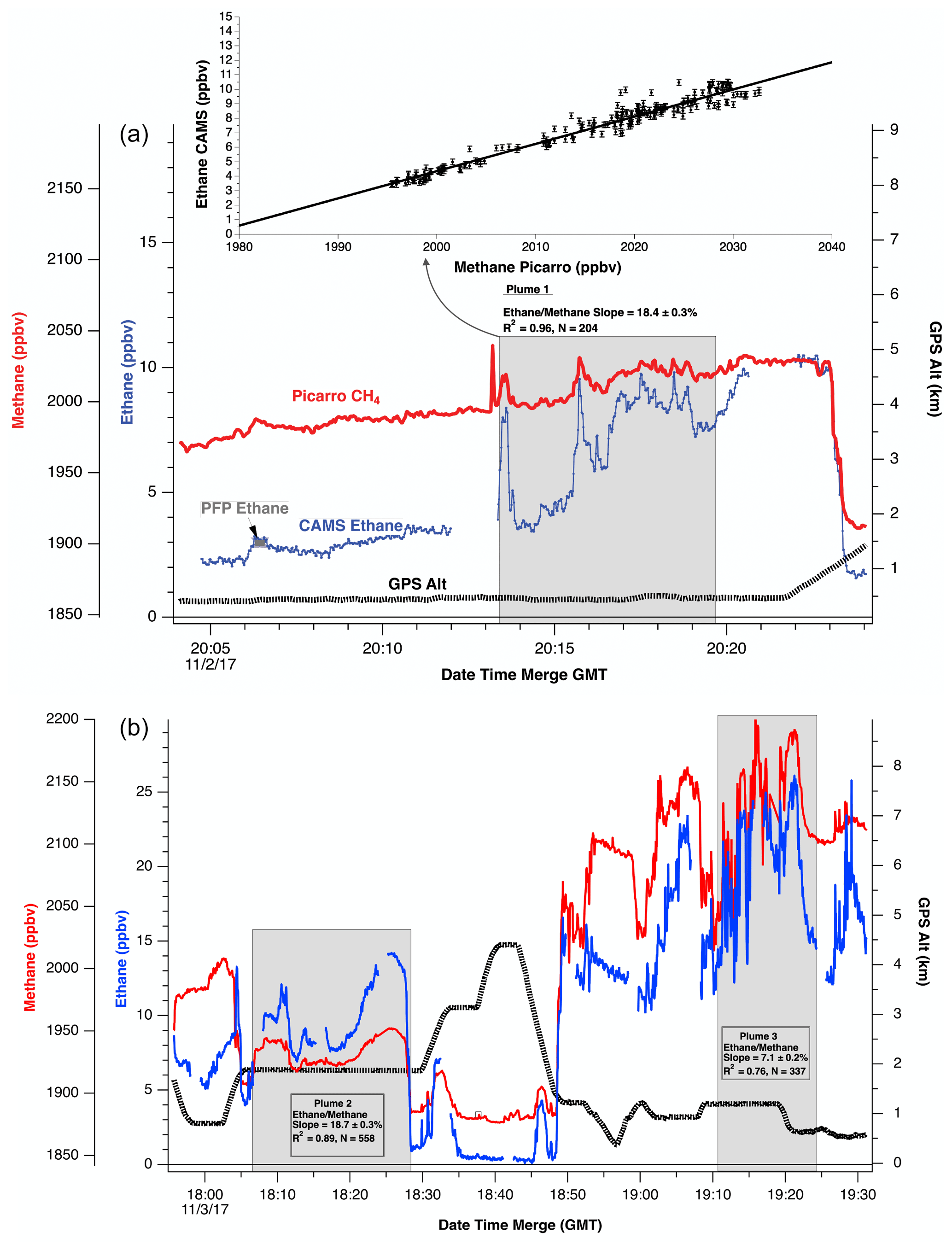
Figure 12(a) Ethane–methane time series plot for plume 1 highlighted in Fig. 11. The CAMS ethane (blue trace) compares well with the PFP ethane measurement shown by the solid gray horizontal points around 20:06. As shown, the ethane–methane slope is 18.4 %. (b) Ethane–methane time series plots for plumes 2 and 3 highlighted in Fig. 11.
3.3 Airborne comparisons of CAMS-2 ethane measurements with NOAA's programmable flask package system
Figure 9a shows a linear regression fit (orthogonal distance regressions, ODRs) of the fast CAMS ethane data averaged over the PFP time base (Y axis) vs. the PFP measurements (X axis), and the results are shown in the ODR inset and in Table 2. During each field deployment (II–IV), we carried out comparisons of our continuous 1 s ethane measurements (not corrected by the calibration standard comparisons) with the NOAA PFP results by averaging our results over the flask fill start and stop times of the PFP system. This procedure is accurate during constant ethane mixing ratios when rapid ethane changes in plumes are not sampled. When sampling plumes, by contrast, one would need to know the exact temporal filling profile of the PFP system in order to modify the CAMS averaging kernel. This is further discussed by Baier et al. (2019). In plumes without taking this into account, one can thus obtain fast averages that are simultaneously too high, too low, and in agreement with the PFP measurements, depending upon the slope of the changes. Thus, to reduce such effects, we exclude CAMS data whose standard deviation over the PFP sampling period is greater than 0.6 ppbv, and the highest point of the regression plot in Fig. 9a (blue point with blue circle) was eliminated for this purpose. As shown in Fig. 9b, the atmospheric ethane (blue lines) and methane (red lines) concentrations were rapidly changing, resulting in PFP underestimations in both cases. The PFP results are highlighted in the shaded region by crosses in both cases. Our 0.6 ppbv ambient ethane standard deviation cutoff filter in this case flagged this point. Here the ambient standard deviation for the CAMS data averaged over the PFP time base was 1.006 ppbv.
The average slope value for the three field deployment phases is 1.030±0.005, which falls within the −1.2 % and +4.8 % range for the calibration standard comparisons. At present, we do not have an explanation for the small but persistent negative intercepts that average to a value of ppbv. This could imply that either the PFP measurements have a small positive interference or the CAMS direct absorption measurements have a small negative interference from the tails of nearby absorptions.
As stated in the Introduction, methane and ethane have common sources from oil and natural gas exploration and production, coal mines, and wildfires. Ratios of ethane and methane measurements can be used to distinguish these sources from biogenic sources of methane. As one example, our CAMS-2 ethane results were employed by Barkley et al. (2019a) to estimate methane emissions using a top-down approach from coal and natural gas production in southwestern Pennsylvania. This research concludes that while Environmental Protection Agency inventories appear to report emissions from coal accurately, emissions from unconventional natural gas are underreported in the region by a factor of 2 to 8. In another example, in Barkley et al. (2019b), ethane–methane slopes from large plumes across frontal boundaries in the midwest are used to differentiate between oil–gas and animal agriculture sources. In this case, the high ethane–methane ratios led to the conclusion that oil and gas sources were responsible for a majority of the unaccounted for methane emissions observed in the frontal flights.
In another application, we show simultaneous ethane and methane measurements over the south-central United States to derive ethane–methane slopes over various shale basins. Figure 10 shows one such example from the southern deployment of the fall 2017 field campaign. Here we show simultaneous enhancements in ethane and methane from the many oil and natural gas exploration and production activities over this region. These include the Permian, Eagle Ford, Barnett, and Haynesville shale regions shown in Fig. 11. This figure employs fast measurements provided by CAMS-2 along with fast methane measurements from a PICARRO methane instrument onboard the B200 to derive ethane–methane slopes shown on the flight tracks as colored points. This plot also shows the gridded methane emissions from the 2012 EPA inventory (Maasakkers et al., 2016) as well as the wind directions and speeds. As can be seen, the ethane–methane slopes over this region are highly variable and range from 0.5 % to 29.1 %. Figure 11 highlights four individual plumes by the black circles surrounding each plume. Figure 12a further shows the ethane and methane time series corresponding to plume 1, while Fig. 12b shows this for plumes 2 and 3. Here the ethane–methane slopes, which range from 7.1 % to 18.7 %, reflect emissions primarily from the Barnett and Eagle Ford shale regions based upon proximity and wind direction. Although we have not yet carried out the same careful shale basin analysis as Peischl et al. (2018) for this region, the ethane–methane slopes in Fig. 11 fall in the same range (8.5 % to 20.5 %) as two study days reported by Peischl et al. (2018) and the 9.6 % reported by Smith et al. (2015).
We present in this study a new autonomous airborne ethane instrument for fast 1 s measurements on the NASA B200 aircraft for ACT-America studies based upon the CAMS-2 DFG spectrometer. This instrument is significantly smaller and lighter-weight than its CAMS-1 predecessor and yields nearly comparable performance within a factor of ∼ 1.3. By operating autonomously, we eliminate the weight of ∼ 110–140 kg typically reserved for an operator and seat. The CAMS-2 instrument employs a pressure-stabilized and thermally controlled enclosure to avoid performance degradation due to aircraft cabin pressure and temperature changes.
This system reliably acquired high-precision and fast ethane measurements on the B200 aircraft over several hundred flight hours during the five ACT-America field campaigns. The airborne performance was significantly improved with each successive field deployment phase study, and we summarized herein the major upgraded design features to achieve these improvements. During the fourth field campaign in the spring of 2018, we achieved 1 s (1σ) airborne ethane precisions reproducibly in the 30–40 parts per trillion (pptv) range in both the boundary layer and the less turbulent free troposphere. To our knowledge, this performance is among some of the best reported to date for fast airborne ethane measurements. In both the laboratory and at times during steady airborne operation these precisions were as low as 15–20 pptv. Comparisons of CAMS-2 with the onboard PFP produced an average slope of ∼ 1.03. It is important to note that our precision estimates and TMU estimates were dynamically determined over the full range of aircraft maneuvers and are thus more representative of instrument performance than a single estimate in a few select conditions.
Measurement data are available at https://doi.org/10.3334/ORNLDAAC/1593 (Davis et al., 2018).
PW, DR, JW, and AF developed, tested, and operated the new instrument during the ACT-America field campaigns. JD, HH, and YC provided the methane measurements discussed in Sect. 4. BB, CS, and BM provided NOAA's portable flask package (PFP) ethane measurements for airborne comparisons discussed in Sect. 3.3. KD, ZB, and MO, in addition to providing critical support for the development activities discussed, also helped in the analysis of ethane–methane slopes discussed in Sect. 4.
The authors declare that they have no conflict of interest.
ACT-America is a NASA Earth Venture Suborbital 2 project funded by NASA's Earth Science Division. We thank the ACT-America scientific and administrative team members, especially the NASA Langley B200 aircraft crew, for their valuable support during the ACT-America field missions.
This research has been supported by NASA's Earth Science Division (grant no. NNX15AW47G).
This paper was edited by Maria Dolores Andrés Hernández and reviewed by two anonymous referees.
Baier, B. C., Sweeney, C., Choi, Y., Davis, K. J., DiGangi, J. P., Feng, S., Fried, A., Halliday, H., Higgs, J., Lauvaux, T., Miller, B. R., Montzka, S. A., Newberger, T., Nowak, J. B., Patra, P., Richter, D., Walega, J., and Weibring, P.: Multispecies assessment of factors influencing regional CO2 and CH4 enhancements during the winter 2017 ACT-America campaign, J. Geophys. Res.-Atmos., 125, 2, https://doi.org/10.1029/2019JD031339, 2019.
Barkley, Z. R., Lauvaux, T., Davis, K. J., Deng, A., Fried, A., Weibring, P., Richter, D., Walega, J. G., DiGangi, J. P., Ehrman, S. H., Ren, X., and Dickerson, R. R.: Estimating Methane Emissions From Underground Coal and Natural Gas Production in Southwestern Pennsylvania, Geophys. Res. Lett., 46, 4531–4540, https://doi.org/10.1029/2019GL082131, 2019a.
Barkley, Z. R., Davis, K. J., Feng, S., Balashov, N., Fried, A., Di-Gangi, J., Choi, Y., and Halliday, H. S.: Forward modeling and optimization of methane emissions in the South Central United States fusing aircraft transects across frontal boundaries, Geophys. Res. 10 Lett., 46, 13564–13573, https://doi.org/10.1029/2019GL084495, 2019b.
Bell, E., O'Dell, C. W., Davis, K. J., Campbell, J., Browell, E., Denning, A. S., Dobler, J., Erxleben, W., Fan, T. F., Kooi, S., Lin, B., Pal, S., and Weir, B.: Evaluation of OCO-2 XCO2 Variability at Local and Synoptic Scales using Lidar and in Situ Observations from the ACT-america Campaigns, J. Geophys. Res.-Atmos., 125, 10, https://doi.org/10.1029/2019JD031400, 2020.
Davis, K. J., Obland, M. D., Lin, B., Lauvaux, T., O'Dell, C., Meadows, B., Browell, E. V., DiGangi, J. P., Sweeney, C., McGill, M. J., Barrick, J. D., Nehrir, A. R., Yang, M. M., Bennett, J. R., Baier, B. C., Roiger, A., Pal, S., Gerken, T., Fried, A., Feng, S., Shrestha, R., Shook, M. A., Chen, G., Campbell, L. J., Barkley, Z. R., and Pauly, R. M.: ACT-America: L3 Merged In Situ Atmospheric Trace Gases and Flask Data, Eastern USA, https://doi.org/10.3334/ORNLDAAC/1593, ORNL DAAC, Oak Ridge, Tennessee, USA, 2018.
Feng, S., Lauvaux, T., Davis, K. J., Keller, K., Zhou, Y., Williams, C., Schuh, A. E., Liu, J., and Baker, I.: Seasonal characteristics of model uncertainties from biogenic fluxes, transport, and large-scale boundary inflow in atmospheric CO2 simulations over North America, J. Geophys. Res.-Atmos., 124, 14325–14346, https://doi.org/10.1029/2019JD031165, 2019.
Harrison, J. J., Allen, N. D., and Bernath, P. F.: Infrared absorption cross sections for ethane (C2H6) in the 3μm region, J. Quant. Spectrosc. Ra., 111, 357–363, https://doi.org/10.1016/j.jqsrt.2009.09.010, 2010.
Helmig, D., Rossabi, S., Huebler, J., Tans, P., Montzka, S.A., Masarie, K., Thoning, K., Duelmer, C. P., Claude, A., Carpenter, L. J., Lewis, A. C., Punjabi, S., Reimann, S., Vollmer, M. K., Steinbrecher, R., Hannigan, J. W., Emmons, L. K., Mahieu, E., Franco, B., Smale, D., and Pozzer, A.: Reversal of global atmospheric ethane and propane trends largely due to US oil and natural gas production, Nat. Geosci., 13, 490–498, https://doi.org/10.1038/NGEO2721, 2016.
Kort, E. A., Smith, M. L., Murray, L. T., Gvakharia, A., Brandt, A. R., Peischl, J., Ryerson, T. B., Sweeney, C., and Travis, K.: Fugitive emissions from the Bakken shale illustrate role of shale production in global ethane shift, Geophys. Res. Lett., 43, 4617–4623, https://doi.org/10.1002/2016GL068703, 2016.
Kostinek, J., Roiger, A., Davis, K. J., Sweeney, C., DiGangi, J. P., Choi, Y., Baier, B., Hase, F., Groß, J., Eckl, M., Klausner, T., and Butz, A.: Adaptation and performance assessment of a quantum and interband cascade laser spectrometer for simultaneous airborne in situ observation of CH4, C2H6, CO2, CO and N2O, Atmos. Meas. Tech., 12, 1767–1783, https://doi.org/10.5194/amt-12-1767-2019, 2019.
Levenberg, K.: A Method for the Solution of Certain Non-Linear Problems in Least Squares, Quart. Appl. Math., 2, 164–168, https://doi.org/10.1090/qam/10666, 1944.
Maasakkers, J. D., Jacob, D. J., Sulprizio, M. P., Turner, A. J., Weitz, M., Wirth, T., Hight, C., DeFigueiredo, M., Desai, M. Schmeltz, R., Hockstad, L., Bloom, A. A., Bowman, K. W., Jeong, S., and Fischer, M. L.: Gridded National Inventory of U.S. Methane Emissions, Environ. Sci. Technol., 50, 13123–13133, https://doi.org/10.1021/acs.est.6b02878, 2016.
Marquardt, D.: An Algorithm for Least-Squares Estimation of Nonlinear Parameters, J. Soc. Indust. Appl. Math., 11, 431–441, https://doi.org/10.1137/0111030, 1963.
Pal, S., Davis, K. J., Lauvaux, T., Browell, E. V., Gaudet, B. J., Stauffer, D.,R., Obland, M. D., Choi, Y., DiGangi, J. P., Feng, S., Lin, B., Miles, N. L., Pauly, R. M., Richardson, S. J., and Zhang, F.: Observations of Greenhouse Gas Changes across Summer Frontal Boundaries in the Eastern United States, J. Geophys. Res.-Atmos., 125, 5, https://doi.org/10.1029/2019JD030526, 2020.
Peischl, J., Eilerman, S. J., Neuman, J. A., Aikin, K. C., de Gouw, J., Gilman, J. B., Herndon, S. C., Nadkarni, R., Trainer, M., Warneke, C., and Ryerson, T. B.: Quantifying Methane and Ethane Emissions to the Atmosphere from Central and Western U.S. Oil and Natural Gas Production Regions, J. Geophys. Res.-Atmos., 123, 7725–7740, https://doi.org/10.1029/2018JD028622, 2018.
Richter, D.: Optical Multipass Cell, US Patent #8,508,740, 2013.
Richter, D., Weibring, P., Walega, J. G., Fried, A., Spuler, S., and Taubman, M. S.: Compact highly sensitive multi-species airborne mid-IR spectrometer, Appl. Phys. B, 119, 119–131, https://doi.org/10.1007/s00340-015-6038-8, 2015.
Smith, M. L., Kort, E. A., Karion, A., Sweeney, C., Herndon, S. C., and Yacovitch, T. I.: Airborne Ethane Observations in the Barnett Shale: Quantification of Ethane Flux and Attribution of Methane Emissions, Environ. Sci. Technol., 49, 8158–8166, https://doi.org/10.1021/acs.est.5b00219, 2015.
Weibring, P., Richter, D., Fried, A., Walega, J. G., and Dyroff, C.: Ultra-high-precision spectrometer II:system description and spectroscopic performance, Appl. Phys. B, 85, 207–218, https://doi.org/10.1007/s00340-006-2300-4, 2006.
Weibring, P., Richter, D., Walega, J. G., and Fried, A.: First demonstration of high performance difference frequency spectrometer on airborne platforms, Opt. Express, 15, 13476–13495, https://doi.org/10.1364/OE.15.013476, 2007.
Weibring, P., Richter, D., Walega, J. G., Rippe, L., and Fried, A.: Difference frequency generation spectrometer for simultaneous multispecies detection, Opt. Express, 18, 27670–27681, https://doi.org/10.1364/OE.18.027670, 2010.
Yacovitch, T. I., Herndon, S. C., Roscioli, J. R., Floerchinger, C., McGovern, R. M., Agnese, M., Pétron, G., Kofler, J., Sweeney, C., Karion, A., Conley, S. A., Kort, E. A., Nähle, L., Fischer, M., Hildebrandt, L., Koeth, J., McManus, J. B., Nelson, D. D., Zahniser, M. S., and Kolb, C. E.: Demonstration of an Ethane Spectrometer for Methane Source Identification, Environ. Sci. Technol., 48, 8028–8034, https://doi.org/10.1021/es501475q, 2014.
Zhou, Z. Y., Ding, D. S., Jiang, Y. K., Zhang, W., Shi, S., Shi, B. S., and Guo, G. C.: Generation of light with controllable spatial patterns via sum frequency in quai-phase matching crystals, Sci. Rep., 4, 5650, https://doi.org/10.1038/srep05650, 2014.
Zhou, Y., Williams, C. A., Lauvaux, T., Davis, K. J., Feng, S., Baker, I., Denning, S., and Wei, Y.: A multiyear gridded data ensemble of surface biogenic carbon fluxes for North America: Evaluation and analysis of results, J. Geophys. Res.-Biogeosci., 125, 2, https://doi.org/10.1029/2019JG005314, 2020.
- Abstract
- Introduction
- Instrument design and setup
- System improvements during each ACT-America airborne field deployment phase and comparisons of CAMS-2 with CAMS-1
- Employing CAMS ethane measurements in assessing methane sources
- Summary
- Data availability
- Author contributions
- Competing interests
- Acknowledgements
- Financial support
- Review statement
- References