the Creative Commons Attribution 4.0 License.
the Creative Commons Attribution 4.0 License.
 | 30 Nov 2020
Effects of clouds on the UV Absorbing Aerosol Index from TROPOMI
Piet Stammes
Victor Trees
Maarten Sneep
L. Gijsbert Tilstra
Martin de Graaf
Deborah C. Stein Zweers
Ping Wang
Olaf N. E. Tuinder
J. Pepijn Veefkind
The ultraviolet (UV) Absorbing Aerosol Index (AAI) is widely used as an indicator for the presence of absorbing aerosols in the atmosphere. Here we consider the TROPOMI AAI based on the 340 nm/380 nm wavelength pair. We investigate the effects of clouds on the AAI observed at small and large scales. The large-scale effects are studied using an aggregate of TROPOMI measurements over an area mostly devoid of absorbing aerosols (Pacific Ocean). The study reveals that several structural features can be distinguished in the AAI, such as the cloud bow, viewing zenith angle dependence, sunglint, and a previously unexplained increase in AAI values at extreme viewing and solar geometries. We explain these features in terms of the bidirectional reflectance distribution function (BRDF) of the scene in combination with the different ratios of diffuse and direct illumination of the surface at 340 and 380 nm. To reduce the dependency on the BRDF and homogenize the AAI distribution across the orbit, we present three different AAI retrieval models: the traditional Lambertian scene model (LSM), a Lambertian cloud model (LCM), and a scattering cloud model (SCM). We perform a model study to assess the propagation of errors in auxiliary databases used in the cloud models. The three models are then applied to the same low-aerosol region. Results show that using the LCM and SCM gives on average a higher AAI than the LSM. Additionally, a more homogeneous distribution is retrieved across the orbit. At the small scale, related to the high spatial resolution of TROPOMI, strong local increases and decreases in AAI are observed in the presence of clouds. The BRDF effect presented here is a first step – more research is needed to explain the small-scale cloud effects on the AAI.
- Article
(14776 KB) - Full-text XML
- BibTeX
- EndNote


Aerosols are small liquid or solid particles suspended in the air. Aerosols have a direct effect on climate because they absorb and scatter solar and terrestrial radiation (e.g., Boucher, 2015; Penner et al., 2001). In terms of radiative properties, two types of aerosols can be distinguished: absorbing and scattering aerosols. Absorbing aerosols, such as smoke from biomass burning, desert dust, volcanic ash, and anthropogenically produced soot, absorb radiation and have a warming effect on the climate. Scattering aerosols, like sulfate particles and clouds, scatter solar light and usually have a cooling effect on the climate. Aerosols also act as condensation nuclei in the process of cloud formation, potentially altering the optical properties of these clouds.
The ultraviolet (UV) Absorbing Aerosol Index (AAI) indicates the presence of absorption in the atmosphere attributed to aerosols. It separates the spectral contrast at two ultraviolet (UV) wavelengths caused by aerosol absorption from that of molecular Rayleigh scattering, surface reflection, and absorption by trace gases (Torres et al., 1998; de Graaf et al., 2005). Ideally, the AAI is zero if there are no absorbing or scattering aerosols present in the scene.
Originally, methods of observing aerosols from space relied on measurements in the visible and infrared regions of the spectrum (e.g., King et al., 1999). In these spectral regions, Rayleigh scattering is less important, and inversion calculations are relatively simple. However, developments in radiative transfer calculations resulted in the possibility of accounting for the multiple scatterings occurring in the UV spectral region which, in turn, allowed for novel techniques of measuring aerosols (Torres et al., 2002). The use of UV radiation for the global detection of aerosols has advantages because in this spectral region, most surfaces are dark, resulting in high contrast with atmospheric effects and a lower sensitivity to aerosol near the surface (Tilstra et al., 2017).
The AAI as an indicator of absorbing aerosols has a strong heritage with retrievals from TOMS (Herman et al., 1997), GOME(-1) (de Graaf et al., 2005), SCIAMACHY (de Graaf and Stammes, 2005; Tilstra et al., 2012), and GOME-2 (de Graaf et al., 2017). The AAI is traditionally defined as the positive values of the reflectance residue between an absorbing-aerosol-loaded atmosphere and a clear atmosphere. Negative values are associated with an atmosphere that contains more scattering particles than a clear atmosphere (Penning de Vries et al., 2009).
Effects of clouds on the AAI were studied earlier using GOME-2 (Penning de Vries and Wagner, 2011) and OMI (Torres et al., 2018; Jethva et al., 2018) data. It was found that using the independent pixel approximation (IPA) instead of a Lambertian scene albedo improves the neutral value of the AAI for scenes with broken clouds.
Besides the monitoring of large aerosol events with TROPOMI, such as the Amazonian wildfires of 2019 and the Australian bushfires of 2019/2020, an important application of the AAI is to preselect scenes for the aerosol layer height (ALH) retrieval of TROPOMI (Sanders et al., 2015; Nanda et al., 2019). Only for scenes with a positive AAI value, the ALH retrieval is performed because the AAI gets positive for increasing amounts of absorbing aerosols and especially for elevated absorbing aerosols (de Graaf et al., 2005). Negative AAI values are mostly associated with scattering aerosols and clouds. Since the AAI is not so much a measure of aerosols but rather a measure of the UV reflectance residue, this paper discusses the current features in the AAI product, which are mainly caused by clouds.
In Sect. 2 we discuss structural features in the AAI at small and large scales. Local features, such as 3D effects and shadows of clouds, are discussed in Sect. 2.2. The large-scale features, such as sunglint, cloud bow, and elevated AAI values near the orbit edges, are discussed in Sect. 2.3. Section 3 discusses in depth the theory behind the observed features and explains the different retrieval approaches discussed in Sect. 3.4, introducing two additional AAI retrieval models to represent clouds. In Sect. 4, we apply the different retrieval models to a selection of TROPOMI orbits. The results are discussed in Sect. 5. Section 6 concludes the work with a summary, a recommendation to users, and prospects of future AAI retrieval improvements.
2.1 Data description
The TROPOMI instrument is a push-broom spectrometer on board the dedicated Sentinel-5 Precursor satellite maintaining a polar orbit with an ascending node Equator crossing at 13:30 local solar time. The TROPOMI AER_AI AAI retrieval (Stein Zweers, 2018) uses level 1b earth radiance measurements converted to reflectances using the ultraviolet–visible–near-infrared band solar irradiance measurements, which have a spectral resolution of 0.5 nm (Ludewig et al., 2020). This study uses a selection of 54 TROPOMI orbits between 6 August and 4 September 2019 over the Pacific Ocean, overlaid and averaged based on the Equator crossing time. The orbits have been chosen in such a way that 178∘ E −140∘ E, where η is the longitude of dayside nadir Equator crossing. We use the TROPOMI offline level 2 AER_AI aerosol index product from the 340 nm/380 nm pair, version 1.2.0, rather than the 354 nm/388 nm pair because of continuity with TOMS, GOME, SCIAMACHY, and GOME-2. However, we do not expect a significant difference in results between the two wavelength pairs. Data are only used if the retrieved scene albedo at 380 nm is between 0 and 1, the solar zenith angle is smaller than 80∘, and the qa_value is > 0.8. This quality assurance value is a continuous quality descriptor, varying between 0 (no data) and 1 (full-quality data). The value is changed based on observation conditions and retrieval flags, and users are recommended to at least ignore data with qa_value < 0.5 (for details see Apituley et al., 2018).
2.2 Small-scale effects of clouds on the AAI
When one zooms in on a TROPOMI AAI map of a scene with broken clouds, one can always see structures of clouds with high and low AAI values. An example is given in Fig. 1, which is a TROPOMI observation over the South Pacific Ocean on 30 August 2018. Please note that no absorbing aerosols are present in this ocean scene, so only clouds can be responsible for the AAI effects.
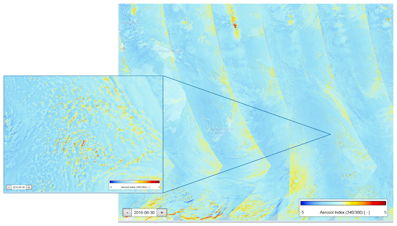
Figure 1Example of small-scale effects of clouds on the TROPOMI AAI over the South Pacific Ocean. This scene was observed on 30 August 2018 (orbit 4563). The large area, about 6000 km× 5000 km centered at around 35∘ S, 170∘ W, contains scattered clouds showing positive (red) and negative (blue) AAI values. The size of the zoomed in area is about 920 km× 760 km.
The small-scale effects show that clouds have sides with high and low AAI. This is related to the small (nadir) pixel size of TROPOMI (3.5 km× 5.5 km), which is in the order of the size of clouds, and not observed by GOME-2 (40 km× 80 km pixels) and OMI (13 km× 24 km pixels).
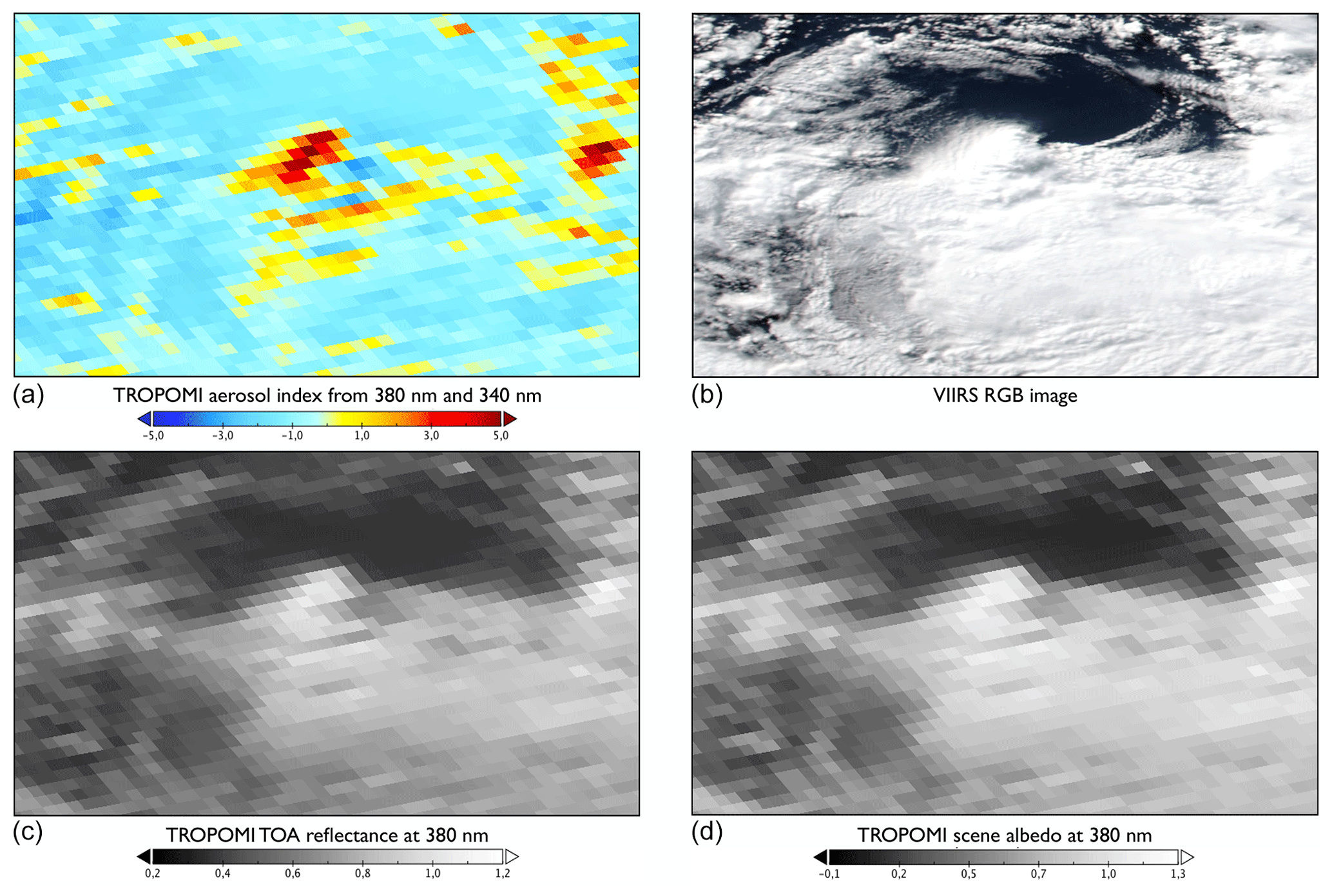
Figure 2TROPOMI AAI (a), VIIRS RGB color image (b), TROPOMI top-of-atmosphere reflectance at 380 nm (c), and TROPOMI-calculated scene albedo 380 nm (d) of a cloudy scene over the South Pacific Ocean (57.3∘ S, 120.4∘ W) on 30 August 2018 (orbit 4562). The size of the depicted area is approximately 245 km× 230 km. VIIRS image credit: NASA/NOAA.
Figure 2 shows the AAI in a cloudy scene over the Pacific Ocean on 30 August 2018 measured by TROPOMI (Fig. 2a). Large positive AAI values are found next to negative AAI values. Comparing the AAI map to the true-color image of Visible Infrared Imaging Radiometer Suite (VIIRS; Fig. 2b), the TROPOMI top of the atmosphere reflectance (Fig. 2c) and the TROPOMI calculated scene albedo at 380 nm (Fig. 2d) shows that the large positive AAI pixels are located at the brightest cloud patches. Stronger negative values are found on the self-shadow side of the clouds (to the right of the cloud tops in this image). Clouds reflect incident sunlight anisotropically, causing a solar illumination and the viewing geometry dependence of the AAI. In Sect. 3.2, we investigate the directional effect of cloud reflection on the AAI.
Negative AAI values are found in the partly clouded area between the thicker clouds. Penning de Vries et al. (2009) showed with plane-parallel cloud modeling that scenes with thin clouds or small geometrical cloud fractions may cause a more negative AAI than cloud-free or fully clouded scenes. In Fig. 2, large negative AAI values are also found on top of the clouds. Indeed, clouds have 3D structures which may induce a self-shadow (i.e., the part of the cloud which is not illuminated by direct light) or a cast shadow (i.e., a shadow on another cloud, the atmosphere, or the surface below the cloud) (Arévalo et al., 2006). At the right side of the brightest cloud patch in Fig 2, the cloud’s self-shadows and cast shadows on lower clouds decrease the AAI. In this work, we will investigate the large-scale cloud effect on the AAI and leave the in-depth analysis of the effect of small-scale and 3D cloud features on the TROPOMI AAI for a future study.
2.3 Large-scale effects of clouds on the AAI
To provide a useful AAI product, the AAI algorithm ideally performs consistently over the orbit, independent of non-aerosol variables, such as solar-viewing geometry, surface properties, cloud presence, and instrumental features. The consistency of the AAI distribution over the Earth can be evaluated by compiling a multi-orbit mean image. This removes the small-scale variability of individual overpasses and reveals structural biases. The Pacific Ocean is mostly devoid of aerosols as it does not harbor any significant natural sources of absorbing aerosols. Any orbits with aerosol plumes from volcanic eruptions or smoke events are not included in the Pacific Ocean data used. The large-scale effect of persistent aerosol contamination is illustrated in Fig. 3 which displays the Pacific multi-orbit AAI on the right and the global AAI on the left. A band of elevated AAI values is seen in the global plot, which can be attributed to plumes of Saharan dust over the Atlantic Ocean. The Pacific is therefore an ideal test environment for AAI features of clouds as we expect the overall AAI mean to be near zero over this region.
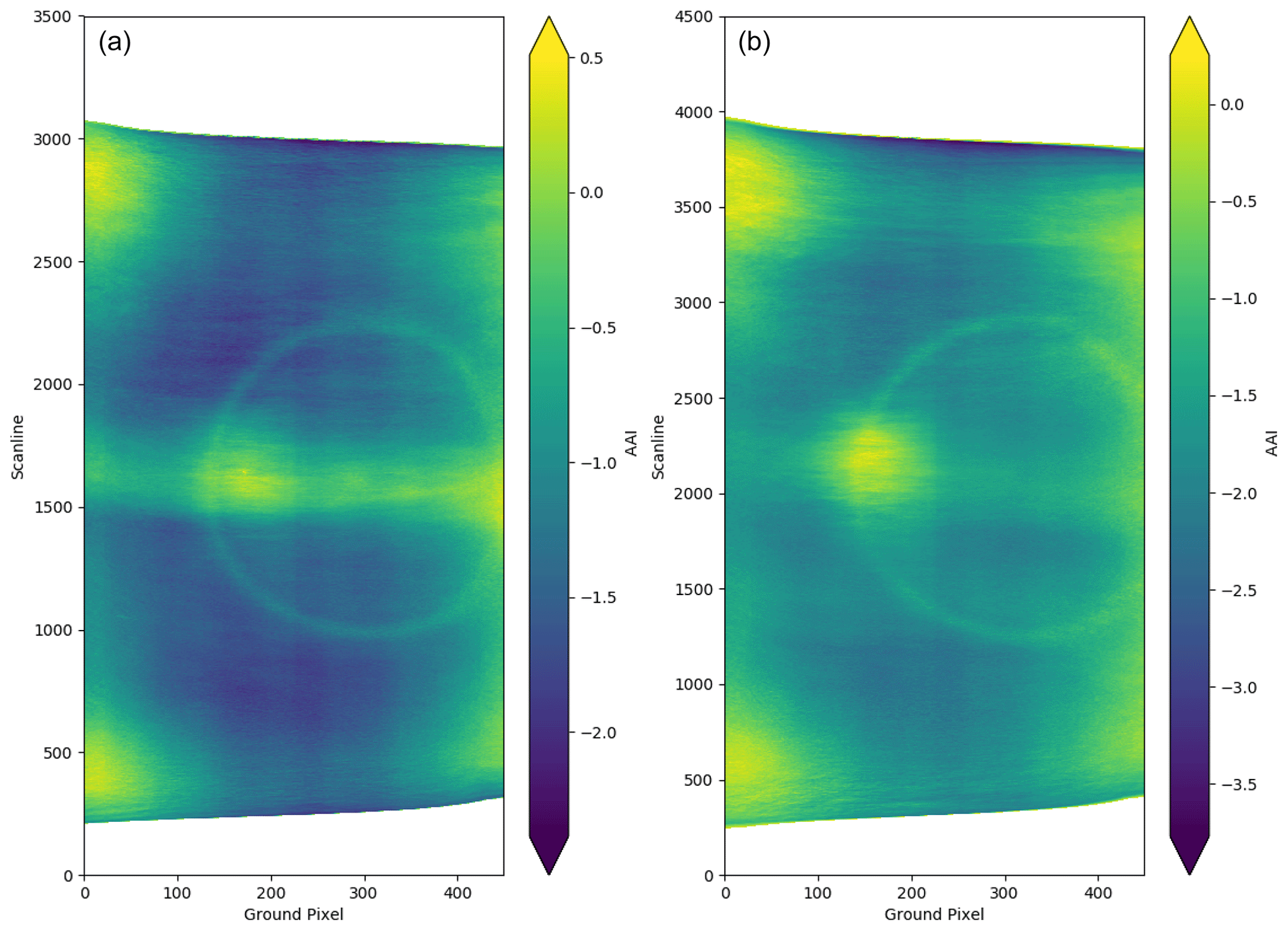
Figure 3Orbital distribution of the TROPOMI AAI averaged over multiple orbits, for global data (a; 103 orbits) and data over the Pacific (b; 54 orbits) in August 2019. The x-axis “groundpixel” represents the viewing direction, whereas the y-axis “scanline” represents the solar position. The contribution of Saharan dust plumes can clearly be seen as a band in the center of the orbit. The Pacific is mostly devoid of absorbing aerosols, and therefore the AAI only shows non-aerosol effects. Note the different color scales.
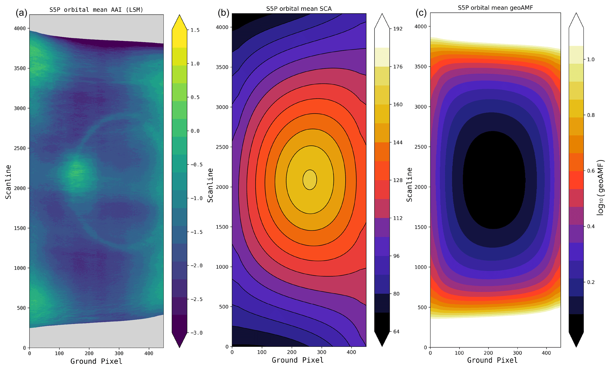
Figure 4(a) Orbital distribution of TROPOMI AAI averaged over 54 orbits over the Pacific. For guidance, panel (b) displays the corresponding single scattering angles, defined as Θ in Eq. (1), and (c) the log10 of the geometric air mass factor, defined as . Positive biases in the AAI are present at the cloud bow, which is at the expected single scattering angle of around 138∘, and at more extreme viewing and solar geometries (large geometric air mass factors).
Figure 4 shows the mean of 54 TROPOMI orbits. The range of values in Fig. 4 immediately shows us that AAI values are mostly negative. This is partly due to the scattering effect of clouds but also due to a radiometric calibration offset and a degradation in the TROPOMI irradiance data. Due to the degradation, the 340 nm/380 nm wavelength pair AAI has dropped by about 0.5 units over the period of 20 months. After sensor commissioning in early 2018, the global average AAI was much higher (). An update of the level 1b product includes an irradiance degradation correction which will alleviate the problem. Activation of the version 2.0.0 level 1b processor is foreseen for late 2020. As the degradation is expected to be independent of viewing geometry, it does not affect the relative AAI values of the orbital features of interest in this work.
The AAI blob in Fig. 4 at the intersection of scanline 2200 and ground pixel 150 is caused by the sunglint which shows up in scenes where the sea surface is visible. The circular pattern intersecting the sunglint can be traced back to the cloud bow when looking at the corresponding single scattering angles. In Fig. 4, the single scattering angle is shown to clarify the geometry-dependence of the AAI. The single scattering angle Θ is defined as the following:
where ϕ−ϕ0 is the relative azimuth angle of viewing and solar directions. Respectively, μ0 and μ are the cosines of the solar and viewing zenith angles.
In Fig. 4a, positive AAI features are found near the orbit edges, especially near the orbit start and end, located at the intersections of ground pixel 0 and scanlines 600 and 3600. The origin of these features is unknown, and we hypothesize that they are caused by a combination of clouds and extreme solar and viewing geometries (i.e., high solar zenith angle, SZA, and viewing zenith angle, VZA).
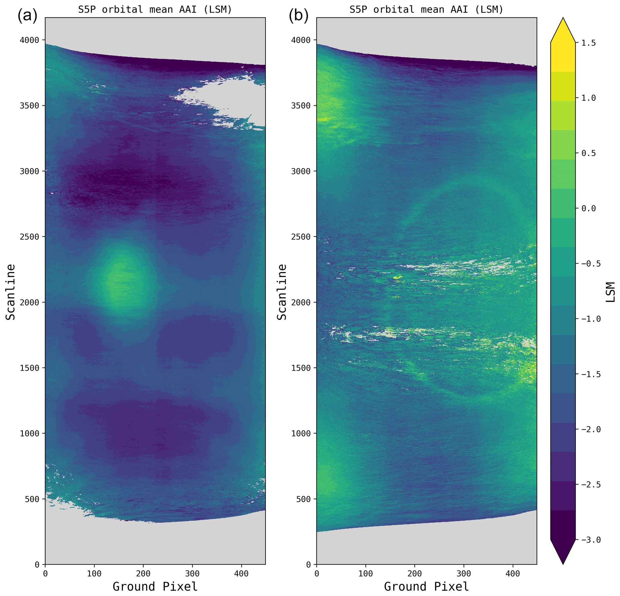
Figure 5Orbital distribution of the TROPOMI AAI based on retrieved scene albedo at 380 nm which is strongly correlated with cloud presence. Scenes with few to no clouds (0.0 < Asc < 0.2) are shown in panel (a), and cloudy scenes (0.6 < Asc < 1.0) are shown in panel (b). Here the same orbits are used as in Fig. 4.
In Fig. 5, the mean orbital distribution of the AAI is shown for scenes with few to no clouds, in which the retrieved scene albedo is small (0.0 < Asc < 0.2), and for cloudy scenes, in which the scene albedo is high (0.6 < Asc < 1.0). The cloudless scenes in Fig. 5a show AAI features due to ocean surface reflection effects, especially the sunglint (the positive AAI blob at ground pixel 130 and scanline 2200), and mildly higher AAI at more extreme viewing angles. The area of strongly negative AAI north and south of the sunglint (around scanlines 1000 and 3000) might also be related to ocean anisotropy (bidirectional reflectance distribution function, BRDF).
The cloudy scenes in Fig. 5b show that clouds play a large role in systematic AAI offsets. Especially the cloud-bow is a prominent feature (centered at ground pixel 280 and scanline 2200 with a radius of approximately 800 scanlines), but we also see enhanced AAI values at more extreme viewing angles. Moreover, a clear increase is seen in the eastern part of the orbit, which is related to the anisotropy of light reflection by clouds.
To assess this hypothesis, we used two more elaborate atmospheric models that compensate for the approximate effect of clouds, similar to Torres et al. (2018). This is described in the next section.
In this section, we first return to the definition of the AAI. Next we consider the effect of the surface BRDF on the AAI. Then we describe the three retrieval models of the AAI. Finally, the radiative transfer model (RTM) used for the AAI calculation and its sensitivities are discussed.
3.1 Definition of the AAI
The AAI is defined as the difference between the ratio of measured reflectances at 340 and 380 nm and the ratio of simulated reflectances at those two wavelengths.
Here the simulated reflectances are calculated for a purely Rayleigh scattering atmosphere without aerosols but including ozone, which is absorbing at these wavelengths. We note that the correction for absorption by ozone, which mainly resides in the stratosphere, can be done accurately since in this part of the UV spectrum (340–400 nm), ozone absorption is weak and does not affect the interaction between aerosols and the molecular atmosphere. For the simulation required in Eq. (2), the albedo of the lower boundary of the atmosphere, called the scene albedo Asc, is adjusted such that the simulated top of atmosphere (TOA) reflectance at 380 nm equals the measured reflectance at 380 nm.
So the scene albedo is the Rayleigh-corrected scene reflectance for an assumed model of the lower boundary, where the default is a Lambertian model. In reality, the scene is generally composed of surface, clouds, and aerosols. The assumption in the AAI retrieval is that the scene albedo is spectrally independent in the spectral window between λ = 380 nm and λ = 340 nm. Thus, the scene albedo that is found at 380 nm is also used for the simulation at 340 nm.
This makes it possible to determine for all scene-specific solar-viewing geometries in order to calculate the AAI according to Eq. (2).
We call the default model for the simulation the Lambertian scene model (LSM). In this model, the surface, clouds, and aerosols in the scene are together represented by one Lambertian surface with albedo Asc. This model is used operationally by TROPOMI (Stein Zweers, 2018) and is used to obtain the results of Sect. 2. The LSM and two other models are further described in Sect. 3.4.
We note that the wavelength pair 340 nm/380 nm can be replaced by another wavelength pair, i.e., 354 nm/388 nm, which is used for OMI (Torres et al., 2002). The longest wavelength of the pair is called the reference wavelength since for that wavelength, the scene albedo is found which is then used for the simulation at the shorter wavelength.
3.2 Effect of anisotropy on the AAI
An important assumption in the default AAI retrieval described above is that the surface is Lambertian, i.e., it reflects isotropically. This means that the directionality of the radiation incident on the surface does not affect the amount of reflection by the surface; direct solar irradiance coming from one direction or diffuse skylight radiation coming from all directions are reflected in the same way. So the assumption is that the total albedo (also called plane albedo) of the surface, averaged over all outgoing directions, does not depend on the directionality of the illumination. However, in reality most surfaces and objects, like clouds, are not Lambertian but reflect anisotropically; they have a bidirectional reflectance distribution function (BRDF) with more reflection in certain directions and less reflection in other directions. According to symmetry considerations, this means that the total albedo of the surface or the cloud layer depends on the directionality of the illumination; for some incident directions the total albedo of the surface or cloud layer is higher than for other incident directions. Thus, an important assumption of the default AAI model breaks down.
The effect of the BRDF on the AAI can be understood as follows. In the UV spectrum, there is a strong spectral dependence of direct and diffuse illumination on the surface since the Rayleigh optical thickness τRay is large and strongly varying: at 340 nm τRay=0.714 and at 380 nm τRay=0.447, which is a ratio of 1.597. The ratio between direct and diffuse downwelling irradiances at the surface (normalized to the incoming solar irradiance at TOA) is 0.358/0.307 = 1.168 at 340 nm and 0.528/0.239 = 2.210 at 380 nm (for SZA = 45∘). So there is almost a doubling of the relative contribution of direct illumination at 380 nm compared to 340 nm. This is due to the much smaller Rayleigh optical thickness at 380 nm which causes a stronger impact of surface BRDF on the TOA reflectance at 380 nm than at 340 nm.
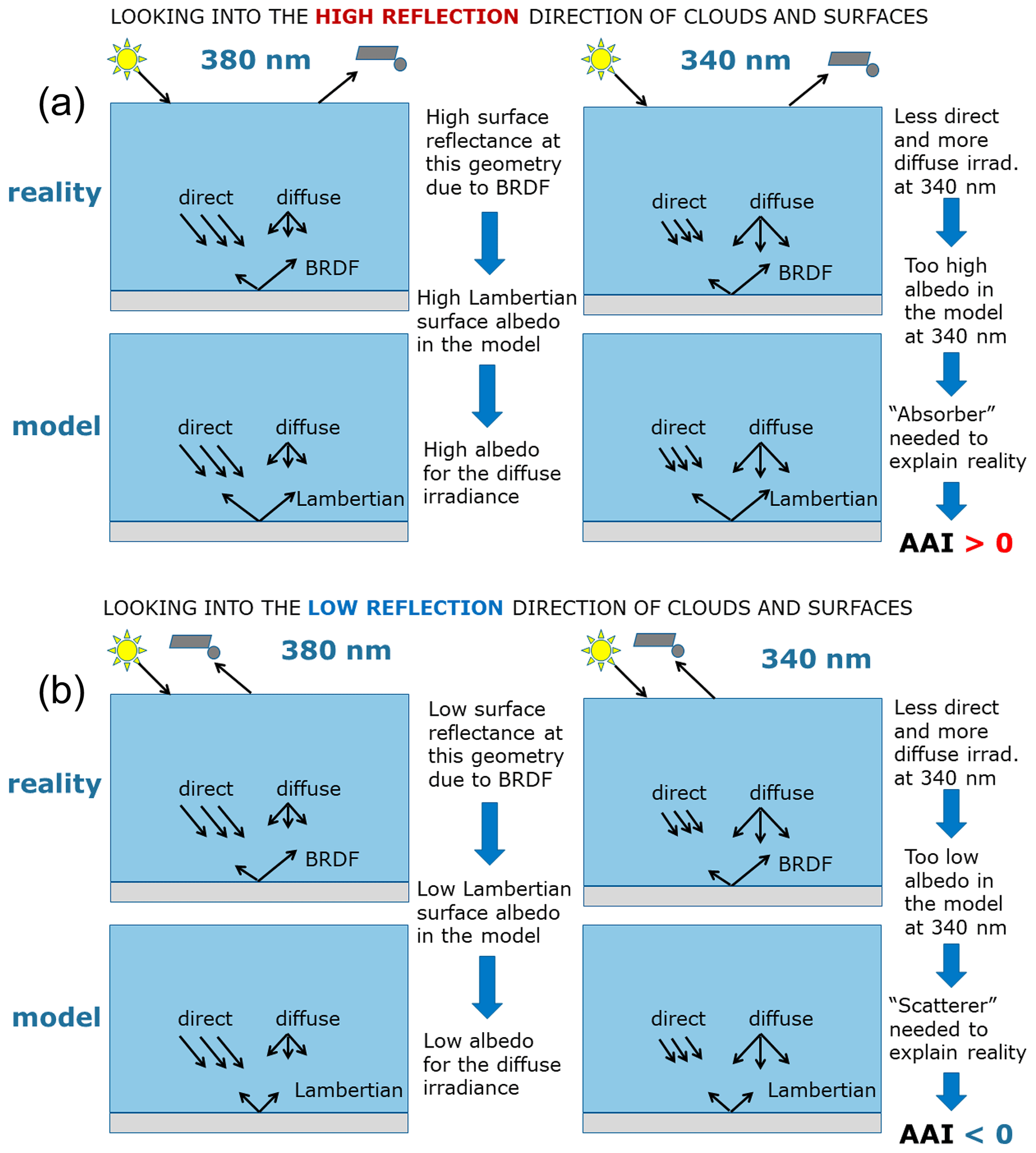
Figure 6(a) The effect of BRDF on the AAI for the high reflection part of the BRDF of the cloud or surface, leading to an enhanced, more positive AAI. (b) Same as panel (a) but for the low reflection part of the BRDF, leading to a reduced, more negative AAI.
The effect on the AAI of this illumination difference in combination with the BRDF is sketched in Fig. 6. Suppose the surface or cloud in the scene has a BRDF with a high and a low reflection part; here we explicitly exclude shadows but only consider the BRDF of a plane surface or cloud. When the satellite is viewing towards the high reflection direction at 380 nm (Fig. 6a) where there is a relatively large direct solar illumination, the high reflectance of the BRDF leads to a high Lambertian scene albedo (cf. Eq. 4). This means that the surface will reflect both direct and diffuse radiation strongly. Then at 340 nm where there is a relatively small direct but relatively large diffuse solar illumination, the model predicts a reflectance at TOA that is too large compared to the observation; thus the AAI becomes positive. In other words, the Lambertian scene albedo that is too high has to be compensated by putting an “absorber” in the atmosphere to match the observed reflectance at 340 nm. This explains the high AAI at the large solar and viewing zenith angles observed in the large-scale effects but also the high AAI value at the bright sides of small-scale clouds. In addition, it explains the high AAI in the sunglint which is an extreme BRDF brightening effect due to Fresnel reflection at the ocean surface under clear sky conditions.
When the satellite is viewing towards the low reflection direction of the surface or cloud (Fig. 6b), the surface reflectance at 380 nm is low, leading to a low Lambertian scene albedo. This same low albedo is used at 340 nm to calculate the model reflectance, but since there is less direct and more diffuse illumination at 340 nm, this leads to a TOA reflectance at 340 nm that is too low. Thus the AAI becomes negative. In other words, “scatterers” have to be added to the atmosphere to compensate for the missing reflectance. In reality, these are expressions of the BRDF of the surface in combination with the different ratio between direct and diffuse illumination at 380 and 340 nm.
3.3 Simulation of AAI of a Mie scattering cloud
As part of the large-scale cloud effects, we clearly observe the cloud bow in the TROPOMI AAI orbital maps. To understand this phenomenon, we have performed a simulation of the AAI of an atmosphere with a Mie scattering cloud which has a droplet size distribution with a 10 µm effective radius. The result is shown in Fig. 7 for three values of the cloud optical thickness (COT), τ, at 380 nm: τ = 1, 8, and 32. In Fig. 7a, the BRDF of the cloud, i.e., the reflection function of the cloud without atmosphere, is shown for a solar zenith angle of 45∘ in the principal plane; in Fig. 7b the calculated AAI is shown for the cloud inside the atmosphere. In Fig. 7b, we clearly see the cloud bow appearing as sharp positive peaks in the AAI for backward scattering directions. This is to be expected on the basis of the discussion above since the cloud bow is part of the BRDF of a Mie scattering cloud. The cloud bow peaks have a similar relative strength of 0.5–1.0 AAI points for all three COT values.
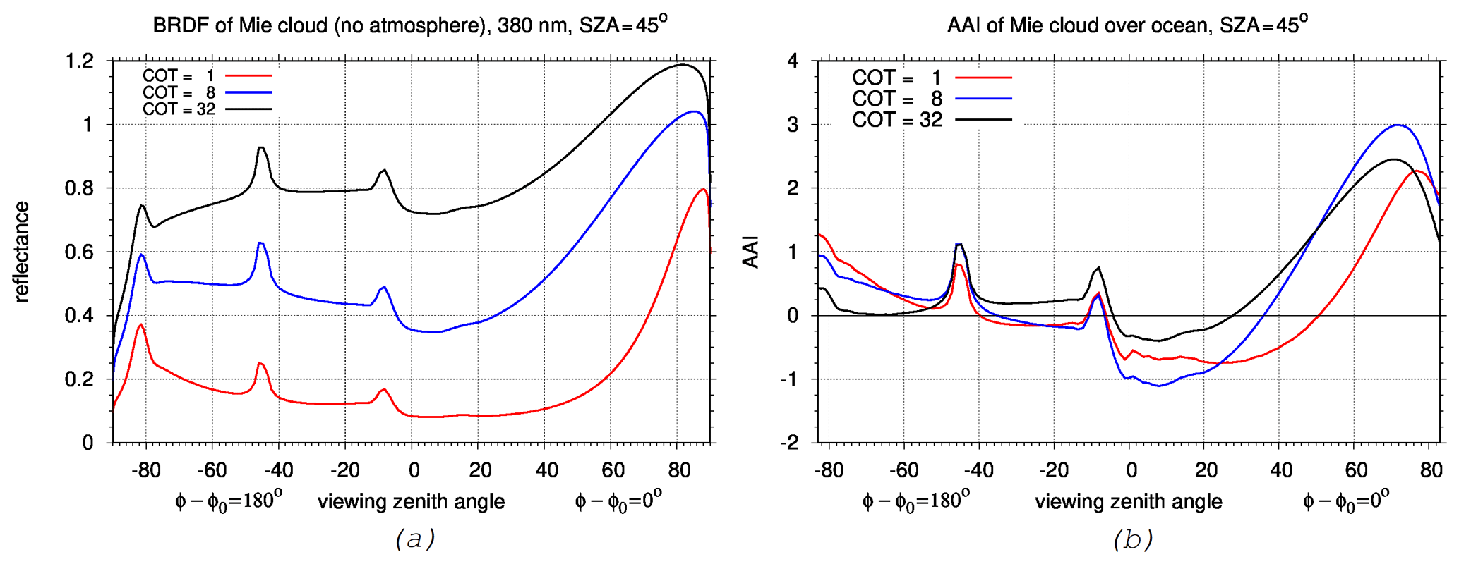
Figure 7(a) Simulated BRDF of a Mie scattering cloud (without atmosphere) as a function of viewing zenith angle in the principal plane for three cloud optical thickness (COT) values: 1, 8, and 32. (b) Simulated AAI of a Mie scattering cloud inside the atmosphere as a function of viewing zenith angle in the principal plane for the same three COT values. The geometric cloud fraction is 1. The solar zenith angle is 45∘. The relative azimuth angle is defined as 0∘ for forward scattering and 180∘ for backward scattering.
In Fig. 7b, we observe a strong slope from negative to positive AAI values towards more forward scattering directions. We speculate that these are the small-scale effects of clouds on the AAI, as shown in Fig. 2. This slope towards a strongly positive AAI for larger viewing zenith angles can also be linked to the large-scale effects since we observe in Fig. 5 an increasing AAI for larger VZA. It appears that the AAI variation versus VZA of a cloud with a large optical thickness (τ=32) is smaller than a cloud with medium optical thickness (τ=8) and small optical thickness (τ=1).
3.4 Three AAI retrieval models
Here we describe the three models of a cloudy atmosphere to simulate the reflectances at the top of atmosphere (TOA) needed in the AAI formula Eq. (2). In Fig. 8, the three models are shown schematically. They have an increasing complexity, starting with the Lambertian scene model (LSM), next the Lambertian cloud model (LCM), and thirdly the scattering cloud model (SCM), consisting of anisotropically scattering particles.
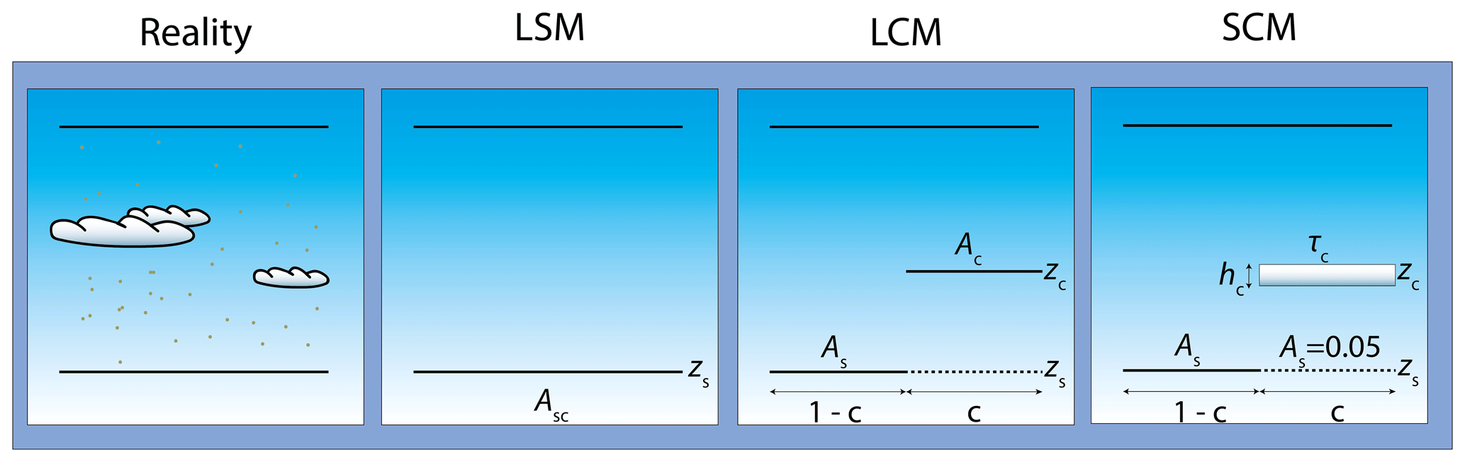
Figure 8Schematic overview of the retrieval scene; zs is the surface height, Asc the scene albedo, c the effective cloud fraction (derived at 380 nm), zc the cloud top height, and Ac the cloud albedo. In the SCM, Ac=0.8, which is determined by a cloud layer thickness hc of 1 km and a cloud optical thickness τc of 28. The fit parameters for the LSM retrieval are Asc and the AAI; for the LCM and SCM retrievals, these are c and the AAI.
3.4.1 Lambertian scene model
The Lambertian scene model (LSM) retrieval is widely used as the default model for AAI retrieval. It describes the scene as a Rayleigh scattering atmosphere bounded by a Lambertian surface (Chandrasekhar, 1960). In this case, the simulated reflectance can be described by the following:
The first term R0 is called the path reflectance and represents solely the atmospheric contribution to the TOA reflectance. The second term represents the combined surface–atmospheric reflectance. The total reflectance Rsim is dependent on a number of parameters: the total O3 column Ω, the albedo of a Lambertian reflector As at surface height zs, the total slant transmittance T, and the spherical albedo of the atmosphere for illumination from below s∗. The cosine of the viewing zenith angle is μ, μ0 is the cosine of the solar zenith angle, and ϕ0−ϕ is the relative azimuth angle between viewing and solar directions.
In the LSM retrieval, the entire scene including surface, clouds, and aerosols is described by one Lambertian reflector. The two observables, R380 and R340, are translated into two retrieved parameters: the scene albedo Asc or Lambertian equivalent reflectivity (LER) and the AAI.
3.4.2 Lambertian cloud model
In the Lambertian cloud model (LCM), two Lambertian reflectors are used: one Lambertian reflector represents the surface and the other Lambertian reflector represents the clouds (Tilstra et al., 2012; Penning de Vries and Wagner, 2011; Torres et al., 2018). The simulated scene reflectance is now constructed as a superposition of a clear sky reflectance Rclr and a cloudy sky reflectance Rcld using the independent pixel approximation (IPA; Marshak et al., 1995):
Here Rsim is the TOA reflectance which is dependent on the viewing geometries μ, μ0, ϕ0−ϕ, surface albedo As, total O3 column Ω, surface height zs, and cloud height zc. The cloud albedo is fixed at Ac=0.8, the assumption of which is also used in the FRESCO cloud retrieval method (Wang et al., 2008, 2012). The parameter c is the radiometric cloud fraction or effective cloud fraction. The wavelength dependence of the reflectances has been omitted in Eq. (6).
The LCM method requires a priori information on surface height and surface albedo for the clear sky part of the scene and information on cloud albedo and cloud height for the cloudy part of the scene. As the clouds are a Lambertian reflector, surface effects underneath are not taken into account.
The effective cloud fraction c can now be determined from the observed and modeled reflectances by requiring that = .
Assuming that c is wavelength-independent between 340 and 380 nm, which is a realistic assumption for clouds, the reflectance at λ = 340 nm is calculated by interpolating the corresponding cloudy and clear sky reflectances from a lookup table (LUT) and applying them to Eq. (6). Next the AAI is calculated for the LCM case following Eq. (2).
It should be noted that in the LCM model, c is fitted instead of Asc in the LSM model. We expect that 0 ≤ c ≤ 1; however, there are good reasons to expect that this is not always the case. The case with c < 0 occurs when the estimated surface albedo is higher than the actual surface albedo. This can happen, for example, in cloud-free scenes when absorbing atmospheric constituents lower the scene reflectance or when the surface albedo database overestimates the actual albedo.
The case of c > 1 can occur, for example, in a cloudy scene when the actual cloud albedo is higher than the (assumed) fixed value for cloud albedo of 0.8. When either of these cases occur, using the LCM is no longer preferred, and instead the algorithm returns to the LSM retrieval. This can be safely done because in these cases the scene is again homogeneous, either fully cloudy or fully clear.
In conclusion, in the LCM retrieval the two observables, R380 and R340, are translated into the effective cloud fraction c and the AAI.
3.4.3 Scattering cloud model
The cloudy atmosphere model can be improved further. Instead of describing the cloud layer as a Lambertian surface, a non-Lambertian cloud model can be used which includes the anisotropic scattering properties of clouds. This is referred to as the scattering cloud model (SCM) retrieval, and it shows similarities with the LCM. The scene is split up into a clear sky part and a cloudy part, and Eq. (6) is used. The main difference is the representation of the simulated reflectances of the cloudy part. Clouds are no longer represented by a Lambertian reflector but rather by a layer consisting of scattering particles.
Cloud particles transmit and scatter radiation with a strong scattering angle dependence. Mie scattering occurs for spherical cloud particles depending on their size distribution. Modeling Mie scattering in a dynamical atmosphere is very challenging because it relies on accurate a priori information about the cloud state. For ice clouds, Mie scattering cannot be used, so other scattering function models are needed. Here, we want to take a simpler approach to include the overall effect of anisotropically scattering cloud particles by resorting to the Henyey–Greenstein (HG) approximation (Greenstein and Henyey, 1941; van de Hulst, 1980). This analytical scattering function approximates realistic scattering characteristics (e.g., a strong forward peak) with the asymmetry parameter g as the only scattering function parameter.
For water clouds, g takes a value of roughly 0.85. However, for ice clouds g is usually between 0.7 and 0.8. In our model, the asymmetry parameter is fixed at g=0.8. Together with the cloud optical thickness, g determines the albedo of the cloud. To get an optically thick cloud with an albedo of about 0.8, which is in line with the FRESCO cloud retrieval algorithm (see Koelemeijer et al., 2001), τ is fixed at 28.
3.5 Radiative transfer model
The simulated reflectances are calculated using the Doubling-Adding KNMI (DAK) radiative transfer model version 3.4.1 (de Haan et al., 1987; Stammes, 2001).
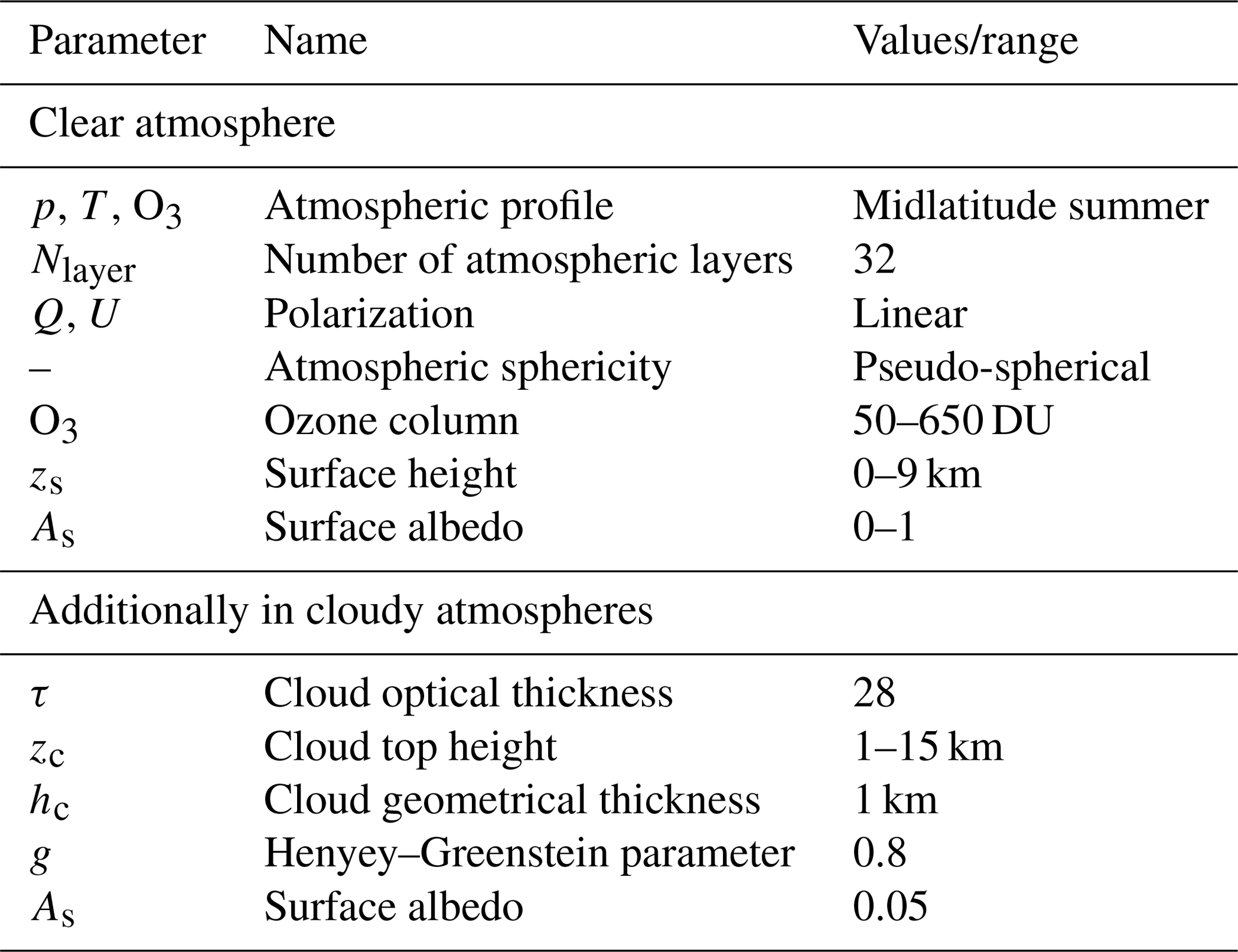
This model computes the monochromatic reflectance and transmittance in a pseudo-spherical atmosphere, including polarization, using the doubling-adding method. For an arbitrary number of layers, which can have Rayleigh scattering, gas absorption, and aerosol or cloud particle scattering and absorption, this method calculates the polarized internal radiation field, as well as the TOA reflectance. For many combinations of viewing geometry, atmospheric state (cloud height, O3 column), and surface state (e.g., surface height and albedo), the TOA reflectances are calculated and stored in a LUT. Model parameter settings are summarized in Table 1. The atmospheric profile of pressure p, temperature T, and ozone mixing ratio is the standard midlatitude summer (MLS) profile (Anderson et al., 1986).
Table 1Parameter settings used for the DAK radiative transfer model for clear and cloudy atmospheres.
3.6 Sensitivity to input parameters
Here the three different AAI retrieval methods are tested for a series of simulated scenes with clouds – but without absorbing aerosols – to investigate their sensitivity to errors in the input parameters. We note that the influence of cloud fraction and cloud optical thickness on AAI has already been discussed in de Graaf et al. (2017) and Penning de Vries and Wagner (2011). Here we study the sensitivity of the AAI algorithm to errors in cloud height and surface albedo. An error (or uncertainty) in any of these inputs will generally result in an error (or uncertainty) in the AAI.
First a baseline scene is defined, upon which one of the parameters will be varied systematically. The baseline scene is a scene 40 % covered by a HG or a Mie scattering cloud with an albedo of 0.8, located between 3 and 4 km altitude (710 and 628 hPa). Figure 9 displays the effect on the AAI if the cloud height is offset. An input cloud top height of 4 km results in an AAI of zero for the SCM retrieval.
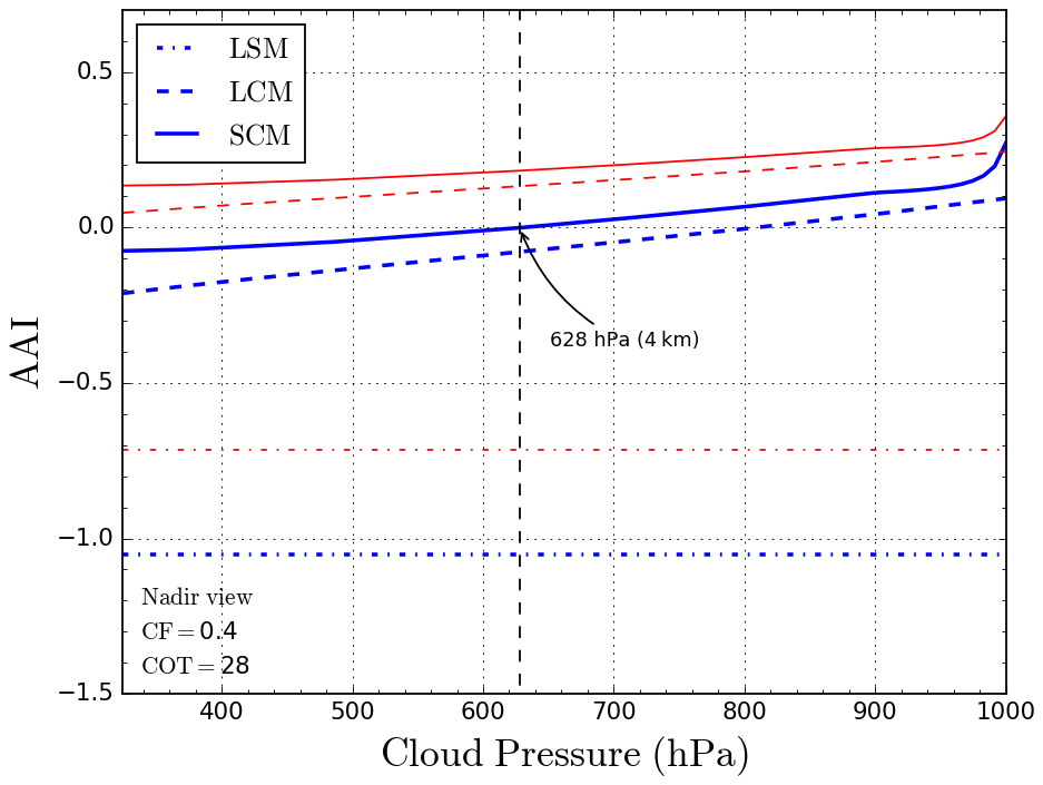
Figure 9AAI sensitivity to errors in the input cloud top pressure for the LSM method (dash-dot), LCM method (dashed), and SCM method (solid) for HG clouds (blue) and Mie clouds (red). Reference cloud pressure is 628 hPa (4 km). The scene has an effective cloud fraction of 40 %.
In case the cloud top pressure is wrongly estimated, for example, if an input value of 500 hPa is given instead of the true value of 628 hPa, the resulting AAI error is about −0.01, as can be read in Fig. 9. Apart from the generally higher AAI values for Mie clouds, the error is similar as for HG clouds. The LCM model results in a shift of about −0.1 AAI compared to the SCM, but errors are very similar to the SCM errors.
Figure 9 shows results for a large range of cloud pressures. Even for large errors in cloud height, the AAI bias in the SCM and LCM is limited to about ± 0.1. For the LSM, there is no dependence of AAI on cloud height since it is not an input parameter. In Fig. 9, the LSM AAI is shifted by about −1 with respect to the SCM AAI for HG and Mie clouds. Typical FRESCO cloud top height errors depend on cloud optical thickness. The FRESCO retrieval works well for optically thick clouds with errors of only a few hundred meters (Wang and Stammes, 2014). Optically thin clouds are harder to detect, and the retrieval yields errors up to 2 km. According to Fig. 9, resulting errors in AAI range from almost zero to 0.1, respectively.
A similar study was conducted to analyze the AAI response to incorrect estimates of surface albedo at 380 nm, which is used in the LCM and SCM retrieval algorithms. Moreover, in this case we assume a scene with 40 % effective cloud fraction. Two cases are analyzed: one with low surface albedo As=0.05, representing forests, deserts, and ocean, and one with high surface albedo As=0.9, representing snow- and ice-covered regions (Tilstra et al., 2017). Results are shown in Fig. 10 and clearly show an AAI dependency on input surface albedo. The LSM retrieval shows a constant AAI value as it is not dependent on surface albedo input. Low albedo scenes are shown in Fig. 10a. In both the LCM and SCM retrievals, a linearly decreasing response to surface albedo is seen of about −0.3 AAI change per +0.1 change in surface albedo. A typical error in the surface albedo database is 0.03 for these types of surfaces, resulting in a potential AAI error of 0.1 index points. High albedo scenes are less sensitive to surface albedo errors on the AAI as shown in Fig. 10b. For surface albedo values above 0.8, the bias is roughly 0.1 AAI index points. When the surface albedo is underestimated, an AAI bias of −0.3 can be observed. As=0.8 presents a singular point since the cloudy and clear parts of the scene are no longer distinguishable, and an asymptote occurs in the AAI. Such high albedo values occur only over snow and/or ice scenes and have a typical error of 0.07, resulting in a potential AAI bias of roughly 0.1.
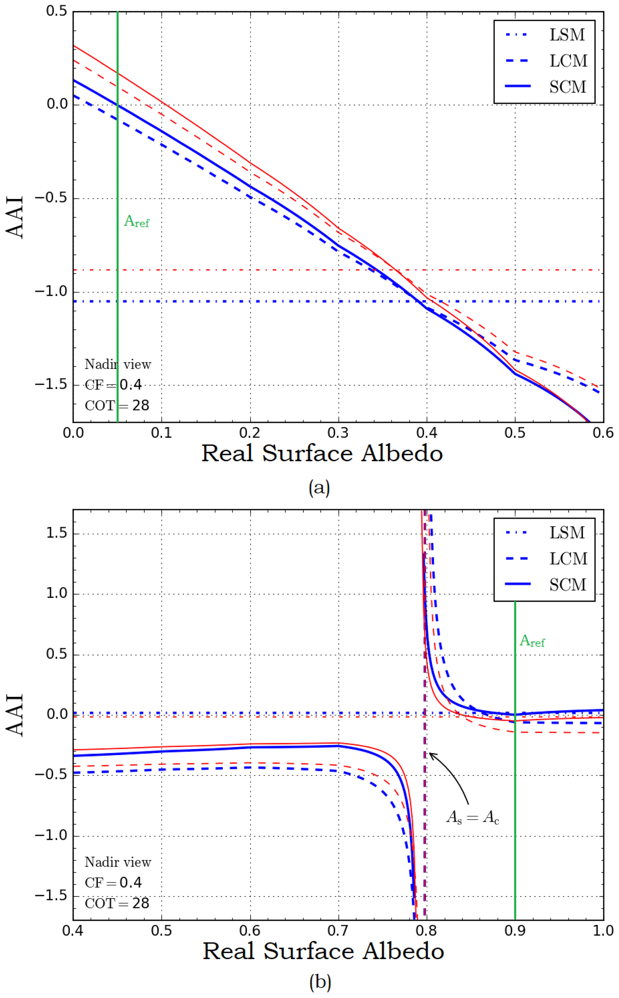
Figure 10AAI sensitivity to errors in surface albedo for the LSM method (dash-dot), LCM method (dashed), and SCM method (solid) for HG clouds (blue) and Mie clouds (red). The green line shows the reference (expected) surface albedo of the scene. The horizontal axis shows the actual (real) surface albedo with panel (a) showing the sensitivity for low albedo scenes with As=0.05 and panel (b) for high albedo scenes with As=0.9. The scene has an effective cloud fraction of 40 %.
Two additional input parameters that potentially affect AAI retrieval accuracy are ozone column and surface elevation. Their influence on the AAI has been researched and is described in de Graaf and Stammes (2005). The typical AAI errors propagated from the input parameters are summarized in Table 2.
Table 2Error range estimates for the AAI retrieval input parameters and their impact on the AAI error range.

4.1 Data selection
The three AAI retrieval methods, LSM, LCM, and SCM, are applied to the same sample of 54 TROPOMI orbits over the Pacific Ocean, as was described in Sect. 2.1.
The LCM and SCM retrievals are dependent on external data sources for the input parameters cloud height and surface albedo. The cloud height data used are generated by the FRESCO algorithm (Wang et al., 2008) which retrieves cloud information from the O2 A-band near 760 nm. Since this information comes from the near infrared (NIR) band, it was regridded to the ultraviolet–visible (UV–VIS) ground pixels. Availability and data quality are not always guaranteed. For example, FRESCO has larger retrieval errors for scenes with very thin clouds or little cloud cover. The surface albedo at 380 nm is taken from the OMI mode LER database which aggregates 5 years of reflectance measurements on a monthly 0.5∘ × 0.5∘ grid, based on Kleipool et al. (2008). In order to ensure that the external input parameters remain within a valid LUT range, the following assumptions are made. If the input surface height is below 0 km (rare occurrence), it is set to 0 km to avoid extrapolation in the LUT. The most significant error would occur in the Dead Sea, as it lies 423 m below sea level. However, this is still well within the vertical resolution of the LUT. Even on the 1 km LUT resolution scale, a terrain height estimate error results in a negligible AAI bias. If the input cloud height is below 1 km (i.e., the cloud is lying on the surface), it is set to 1 km. The RT model does not allow a cloud altitude below 1 km as the thickness of the cloud layer is 1 km.
4.2 AAI behavior along cross sections
To analyze the performance of the three different AAI retrieval models, we again look at the orbital means over the Pacific. The cloud models are sparse on data in the northeastern part of the orbit. This is due to a selection based on surface albedo. Since the surface albedo database is on a 0.5∘ × 0.5∘ grid, it often does not represent the small TROPOMI ground pixels well enough, resulting in large errors. To resolve this problem, we have selected pixels only over the ocean for the LCM and SCM models by removing scenes with a surface albedo database values larger than 0.2 (mostly scenes over Alaska and Antarctica).
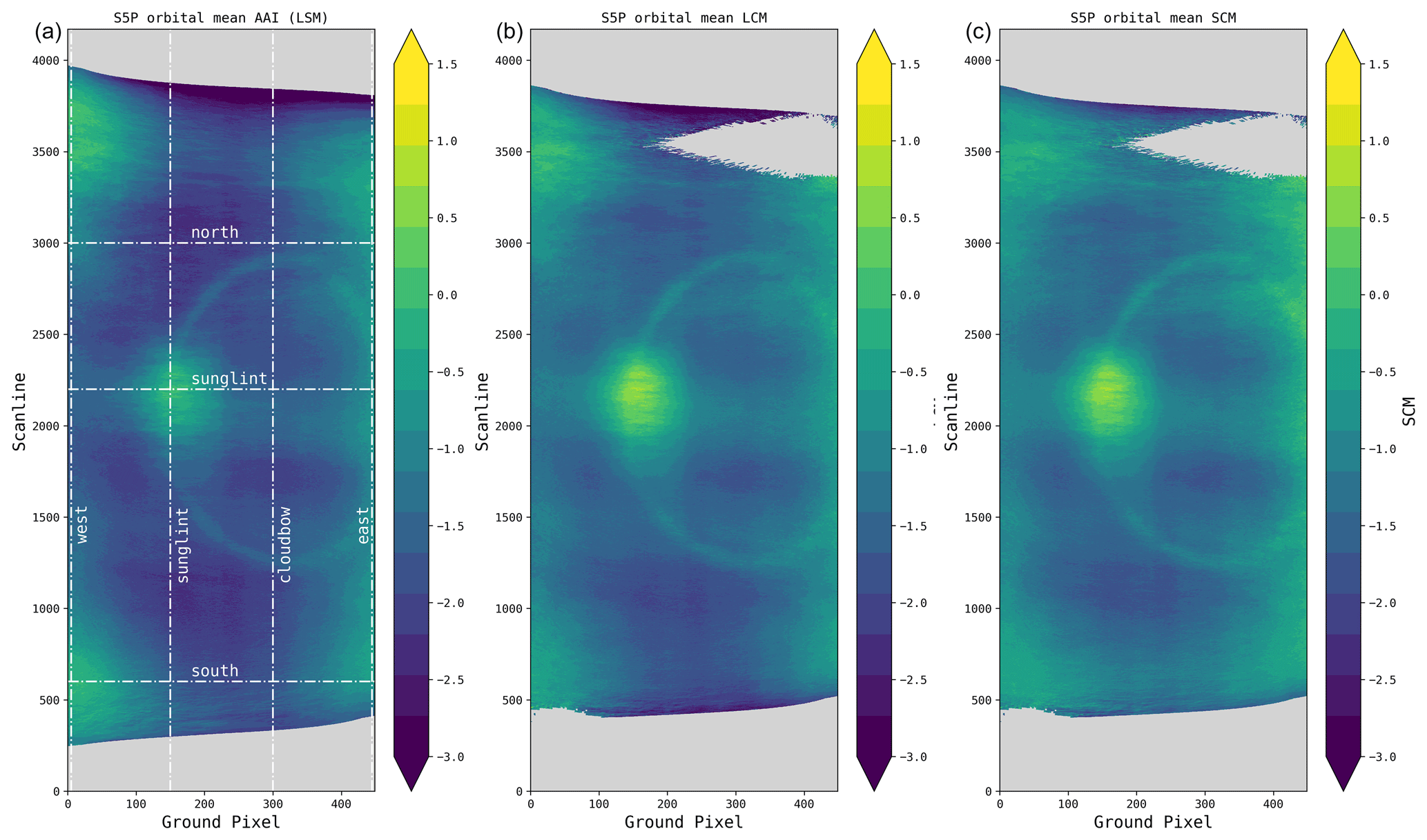
Figure 11Mean orbital distribution of (a) the original TROPOMI AAI retrieval using the LSM method, (b) the LCM retrieval, and (c) the SCM retrieval. The dashed white lines indicate the cross sections used in Figs. 12 and 13. Panels (b) and (c) clearly show a more homogeneous field than the original AAI retrieval. Here the same 54 orbits over the Pacific are used as in Fig. 4a; all cloud fractions are included.
A thorough analysis can be performed by investigating several cross sections. In Fig. 11, the horizontal lines show east–west cross sections of the south, sunglint, and north in such a way that the end-of-orbit feature (“south”), the sunglint (“sunglint”), and no abnormality (“north”) are captured. The vertical lines show (from left to right) the “west”, sunglint, “cloudbow”, and “east” cross sections.
4.2.1 East–west cross sections
Figure 12 shows AAI values for the three east–west cross sections defined in Fig. 11. The north cross section does not intersect any features. An increase can be seen on the east side, which holds for all latitudes and which is associated with the viewing zenith angle dependence of the AAI, as discussed in Sect. 3.3. In this unbiased cross section, compared to the LSM, the LCM (+0.38) and the SCM (+0.59) display on average a higher AAI. The sunglint cross section shows very similar behavior between the LCM (+0.4) and SCM (+0.47) when compared to the LSM. Aside from the overall increase, the sunglint feature does not show any differences between the three retrieval models.
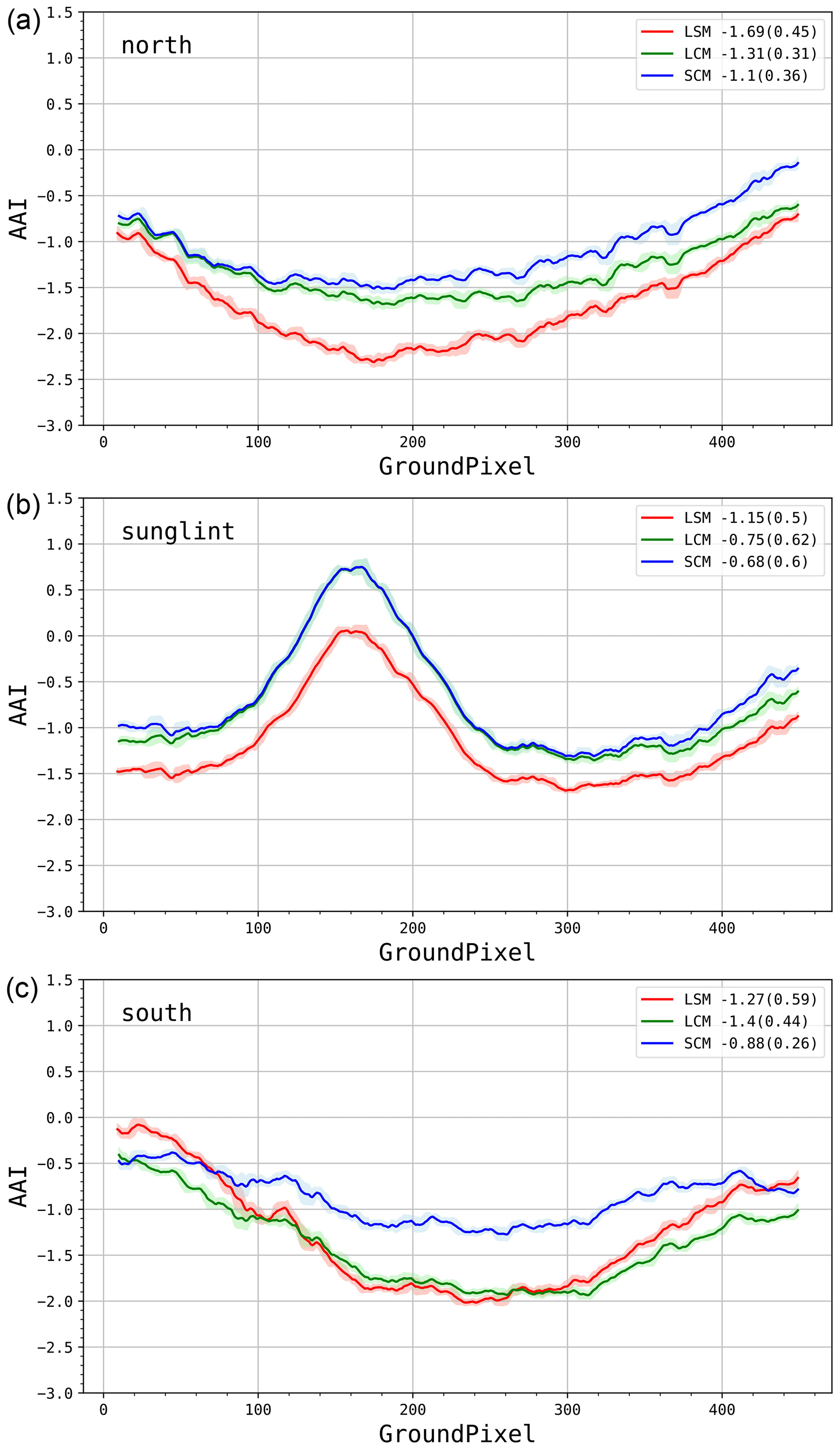
Figure 12TROPOMI AAI as a function of ground pixels for the north (a), sunglint (b), and south (c) east–west cross sections. The three different models are shown: LSM (red), LCM (green), and SCM (blue). The numbers in the legend show the 10-pixel rolling mean and standard deviation (between brackets).
The south cross section runs through the end-of-orbit features on both sides. Compared to the LSM, a strong increase in mean AAI is observed for the SCM (+0.39), whereas the LCM (+0.13) shows similar results. Across-orbit homogeneity of the AAI, in terms of standard deviation, shows large differences, especially in the south cross section that intersects the end-of-orbit features. In the SCM, variability is reduced by 56 % compared to the LSM. This result supports our hypothesis that the SCM improves AAI homogeneity in certain parts of the orbital field.
4.2.2 North–south cross sections
Figure 13 shows AAI values for the three north–south cross sections defined in Fig. 11. It must be noted that at very large scanline numbers, the LCM and SCM do not yield data due to invalid cloud or surface albedo input data, as can be seen in Fig. 11. At very large air mass factors, a sharp decline in AAI values is observed in all models. The east cross section displays on average the highest AAI due to the viewing geometry bias described in Sect. 3.3. The largest AAI mean is retrieved with the SCM, followed by the LCM and the LSM. The same holds for the sunglint, cloudbow, and west cross sections. Noteworthy is the behavior of the three retrievals in the west cross section. A clear reduction in along-track variability is observed for the cloud models, with the LCM and SCM showing a reduction of 35 % and 57 %, respectively, compared to the LSM.
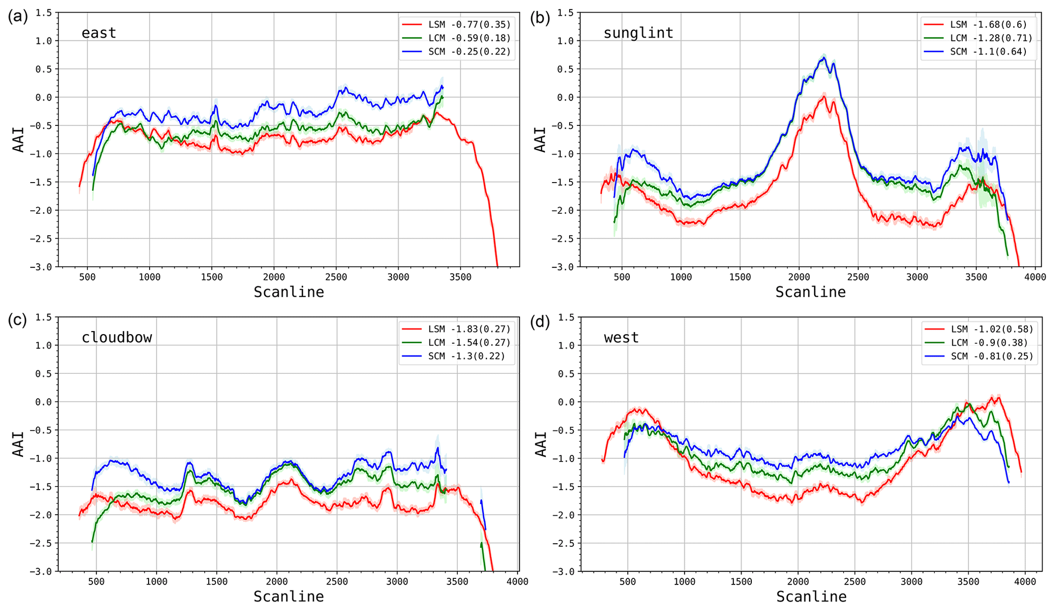
Figure 13TROPOMI AAI as a function of scanline for the east (a), sunglint (b), cloudbow (c), and west (d) north–south cross sections. The three different models are shown: LSM (red), LCM (green), and SCM (blue). The numbers in the legend show the 25-pixel rolling mean and standard deviation (between brackets).
The north–south transect over the sunglint shows a steep behavior, from strongly negative AAI values around scanline 1000 to positive AAI values at the sunglint around scanline 2200 and then again strongly negative AAI values around scanline 3000. The east–west transect over the sunglint in Fig. 12 shows a similar behavior. This steep AAI behavior was earlier mentioned when discussing the cloud-free panel in Fig. 5. This behavior is probably due to ocean BRDF effects because outside the sunglint region, the ocean is very dark (see e.g., Gatebe et al., 2005).
4.3 Differences in orbital distributions
Figure 14 shows that the LCM and SCM retrieve a higher AAI value over a large range of latitudes compared to the LSM. The sunglint is enhanced in both models, as well as midlatitude regions (centered around scanlines 750 and 3000). As clouds typically induce a negative AAI, this increase is likely due to the improved cloud model. At extreme viewing geometries, both cloud models show a decrease in AAI. However, the SCM shifts this decrease mostly toward the regions where we find the end-of-orbit features.
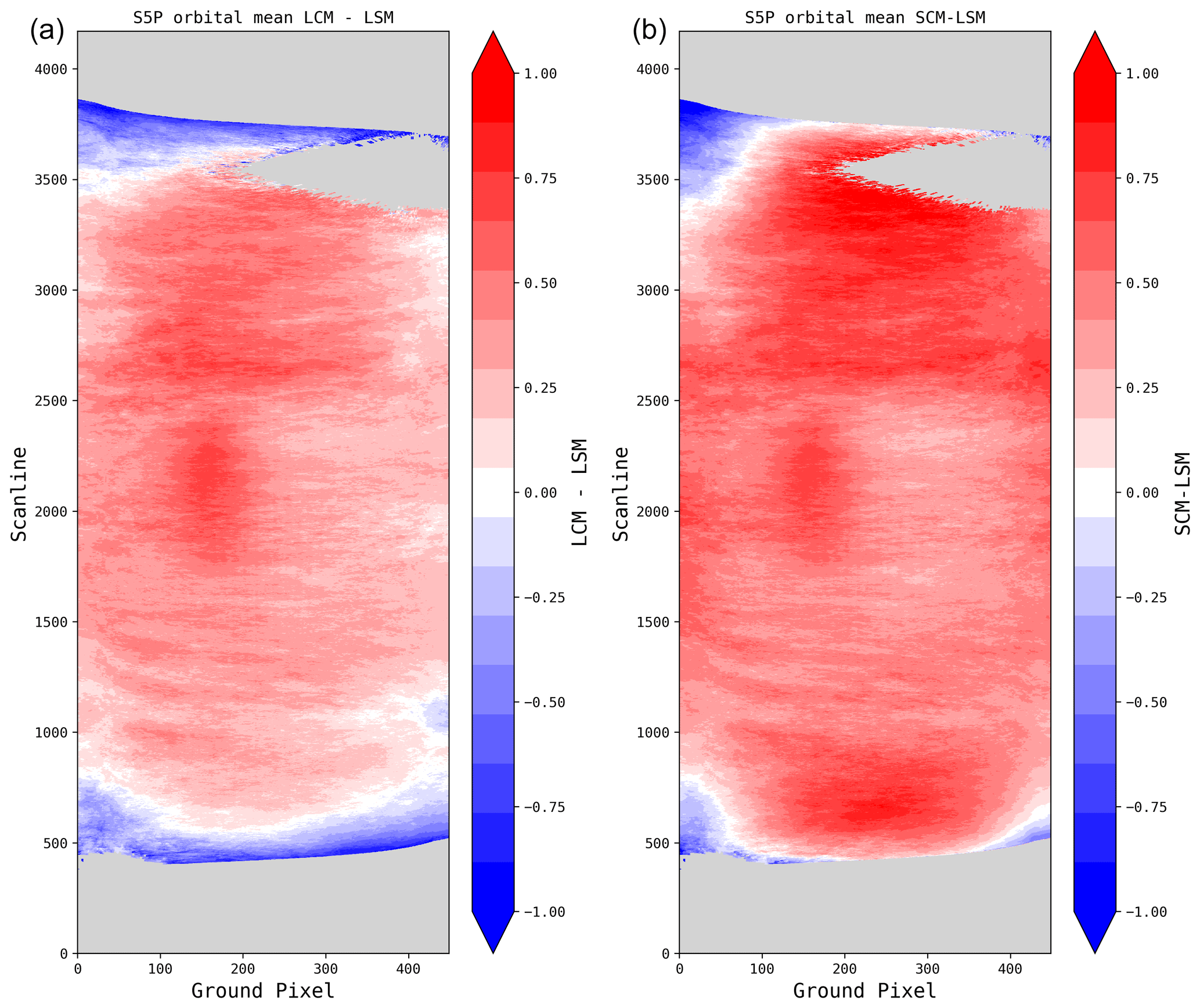
Figure 14Mean difference in orbital distributions of TROPOMI AAI for the LCM (a) and the SCM (b) compared to the original LSM retrieval. Red indicates positive differences and blue negative differences.
4.4 Histograms of the three models
Figure 15 shows histograms of the AAI value occurrence over the orbits for the different retrieval models. The LSM shows a sharp peak at −1.8 and shoulder-like features on the right side of the histogram which are associated with the sunglint, the positive features at the end of orbit, as well as the cloud bow and the elevated values at the eastern side of the orbit, as shown in Fig. 4. A clear shift in the mean is observed for the LCM (+0.3) and SCM (+0.4) retrievals. The standard deviation of the three curves are very similar at 0.5, 0.7, and 0.6 for, respectively, the LSM, LCM, and SCM. However, the shape of the curves give additional insight into the differences. The AAI value cutoff on both sides is relatively sharp in the LSM but shows a more gradual decrease in the LCM and LSM models. The left side of the LCM and SCM histograms can be traced back to the AAI decrease at the orbit ends in Fig. 14. The right side of the histograms relates to the increase in sunglint signal. The shoulder-like features mentioned above are less pronounced in the LCM and LSM, suggesting a more homogeneous distribution for the majority of observations.
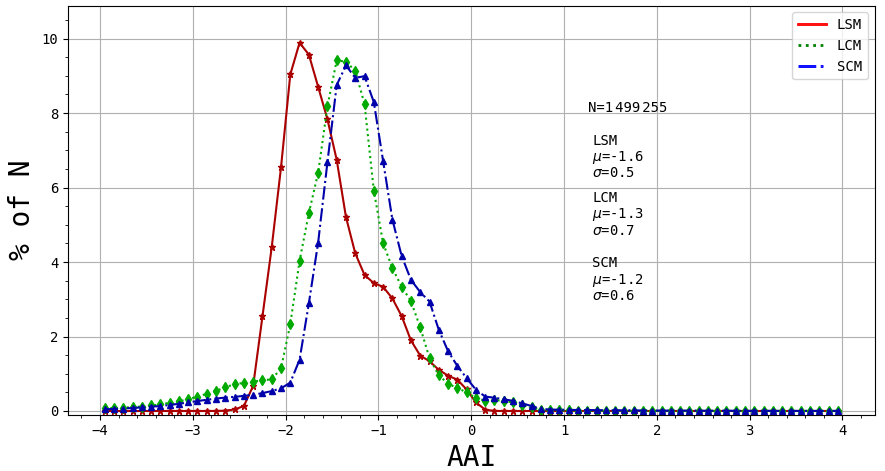
Figure 15Histograms of the AAI value occurrence in the LSM (red), LCM (green), and SCM (blue). The vertical axis displays the percentage of total measurements. The mean μ and standard deviation σ of each histogram are given in the legend. N is the total number of pixels.
4.5 Aerosol event over the Pacific
In Fig. 16, we show how the three AAI retrieval models are performing in the case of absorbing aerosol presence to make sure that the absorbing aerosol signal is still captured. In January 2020, a large plume of smoke from Australian forest fires was transported thousands of kilometers eastwards across the Pacific, reaching the area that we previously used to determine the large-scale cloud effects. The smoke plume has AAI values well above 12. Apart from a small overall increase in AAI values, the smoke plume is very similar across the three models. This allows us to conclude that the absorbing aerosol signal is well captured by all three models.
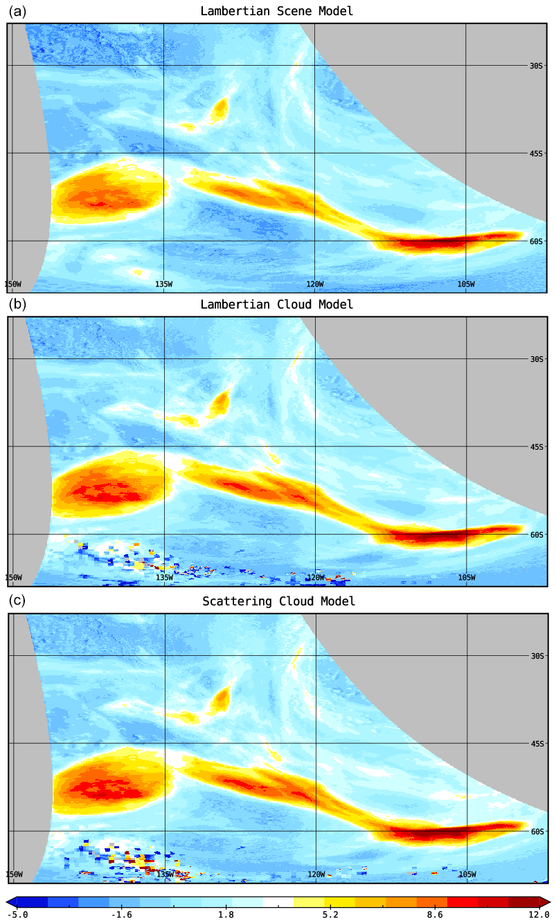
Figure 16TROPOMI AAI of a smoke plume retrieved with the LSM (a), LCM (b), and LSM (c) over the South Pacific Ocean on 4 January 2020. A multitude of persistent forest fires in eastern Australia caused this large absorbing aerosol plume that was transported thousands of kilometers eastwards. The noise in the bottom of the LCM and SCM plots is caused by albedo artifacts due to melting and moving ice. There is hardly any discernible difference in the AAI plume for the three models. For this plume, the AAI values peak at 12.2 (LSM), 13.9 (LCM), and 14.3 (SCM).
In the previous sections, we have presented TROPOMI observations of the large-scale and small-scale effects of clouds on the AAI. The large-scale effects show that the AAI increases over clouds towards more extreme viewing directions and solar directions, i.e., at the edges of the swath and close to the poles. This behavior has also been observed by GOME-2 and OMI (see e.g., de Graaf et al., 2017). The AAI also increases for the cloud bow direction, which leads to a conspicuous circular feature when averaged over many orbits with the same sun-view geometry. In Sect. 3, we have shown that the BRDF of clouds in the scene have a strong impact on the AAI. To cope with the effect of clouds, we have used three different models of the scene in the AAI calculation which have an increasing complexity.
For the data analysis, we selected orbits over the Pacific Ocean, so apart from clouds, only the ocean surface can contribute to the reflectance. At 380 nm, the ocean surface albedo is typically only about 0.08 (Tilstra et al., 2017). Therefore, in (partly) cloudy scenes, the impact of clouds will surpass that of the ocean except in the glint region. As discussed in Sect. 3, in the absence of absorbing aerosols, it is not the absolute reflectance of clouds, ocean, or land that counts for the AAI but the difference in reflectance between bright and dark regions of the BRDF of the scene; for the cloud-free ocean, this means that the BRDF difference between sunglint and non-sunglint regions determines the AAI. We note that possible spectral effects of dissolved matter and chlorophyll in the ocean are not expected since the content of these constituents is very small in the open ocean.
The results of Sect. 4 show that the AAI behavior of the most complex model with a scattering cloud (SCM) produces the flattest AAI field over the orbit. This is a good result, and it was expected given the explanation in Sect. 3 of the effect of the cloud BRDF on the AAI. The impact of errors in the input parameters for the SCM model is only small, as was shown in Sect. 3.6.
The current TROPOMI L1b calibration bias (including degradation) causes a negative shift in the AAI. However, this shift is independent of solar and viewing geometry. So the calibration bias reduces the AAI at a global level, but it does not change the differences in AAI. Therefore, it does not impact our study of the orbital distribution of the AAI.
From the histograms shown in Fig. 15, it appears that the width of the AAI distribution – thus the variability of the AAI – does not become narrower when we improve the model going from LSM via LCM to SCM. The width stays largely the same, and only the mode is shifting towards more positive AAI values. So the SCM is not solving the problem of the wide range of positive and negative AAI values in cloudy, non-aerosol scenes over ocean.
To explain this, we may return to Sect. 3 where we demonstrated that the BRDF of the scene determines the AAI in the absence of aerosols. Therefore, only if we know the BRDF of the scene can we expect to have an optimal AAI retrieval. An optimal AAI retrieval would mean that clouds give a neutral AAI, i.e., close to or equal to zero, and only absorbing aerosols are detected with a positive AAI.
In the SCM model, we have fixed the BRDF of the clouds in the scene to that of a thick cloud with an albedo of 0.8 since we fixed the cloud optical thickness value to COT = 28. However, the BRDF strongly depends on COT; Fig. 7 shows that a thick cloud (COT = 32) has a smaller effect on the AAI than a medium-thick cloud (COT = 8) or a thin cloud (COT = 1). Furthermore, the effective cloud fraction retrieved for such a thick cloud is small and typically half of the geometric cloud fraction (Wang et al., 2008). As a result, the impact of the cloud BRDF on the scene BRDF in Eq. (6) is relatively small in this model.
To obtain the BRDF of the scene itself, retrieving both the geometric cloud fraction and the cloud optical thickness before the AAI can be determined would be required. This requires auxiliary cloud information, which could, e.g., be obtained from VIIRS co-located cloud imagery. However, this would mean a totally different approach; in this way, the elegance and simplicity of the AAI retrieval would be lost. Then the AAI could not be used as a quick filter method to indicate aerosol scenes.
The choice of COT = 28 in the SCM model was done in an analogous way to the cloud model assumption in trace gas retrieval algorithms, which use a thick cloud with an albedo of 0.8 in order to simulate the observed air mass in the atmosphere (Stammes et al., 2008). Another choice for the fixed COT value could be made instead of COT = 28. For example, Torres et al. (2018) use COT = 10 for a Mie scattering cloud, which is more an average COT value based on the median observed COT from MODIS observations. It would be necessary to experiment with which COT value would be optimal to get the lowest spread of AAI values without introducing AAI artifacts like cloud bows and forward scattering effects due to the specific cloud model assumptions.
In the current GOME-2 AAI retrieval, the large-scale effects of clouds on the AAI are corrected for in an empirical way; an empirical model that includes the end-of-orbit features, as well as the across-track smile, is constructed. Then, the orbital mean AAI is monitored over multiple preceding days and fitted to this model. The resulting model fit is subtracted from the newly retrieved AAI orbit. However, the disadvantage is that other effects, like of real aerosols, might accidentally be included in the model and as a result be diminished in this way. Moreover, an AAI data record is required to determine this offset (de Graaf et al., 2017).
The discussion above means that the small-scale effects have also not changed drastically (figure not shown). As we saw above for the large-scale effects of clouds in the many-orbit average AAI, in the small-scale zoomed in AAI fields the value of the AAI is higher in the LCM and SCM cases than in the LSM case, but the variation in AAI for the three models is similar. This can only be reduced by compensating in the individual scenes for the BRDF effects of clouds. In addition, the small-scale effects are also affected by the 3D effects of clouds, like shadows. This is beyond the current discussion, and we leave this for future research.
We have investigated cloud-related features in the TROPOMI AAI from the 340 nm/380 nm wavelength pair. Small-scale features resulting in strong local AAI gradients can be traced back to the presence of clouds and particularly to the cloud BRDF, as well as self-shadowing and cast-shadowing effects.
Large-scale features due to cloud presence in the observed scenes, such as the cloud bow, viewing angle dependence, and end-of-orbit features, have also been investigated. These can be explained by the BRDF of clouds in combination with the different ratio of direct to diffuse illumination of the surface at 380 and 340 nm.
We have attempted to homogenize the AAI distribution along the orbit by introducing two different retrieval models compared to the operational LSM model. A more homogeneous AAI distribution is retrieved when using the LCM and even more so when using the SCM approach. On average, the mean AAI values increase by 0.23 and 0.47 AAI units for LCM and SCM, respectively, mitigating the AAI reduction due to cloud presence.
To conclude which of the three models, LSM, LCM, or SCM, is best remains a matter of choice. It is the dilemma between a more physical retrieval for the AAI with more and more assumptions for the scene against a more simple retrieval with the minimum amount of assumptions. We advocate to keep the elegance of the simple AAI retrieval of the LSM model as an indicator of absorbing aerosols, although with effects of clouds and other BRDF effects included. However, we think it is advantageous to have in addition a correction for the average large-scale BRDF effects of clouds with a model like the SCM with a small amount of cloud assumptions in which a fixed COT and simple scattering phase function are used. The optimal choice of these parameters will be investigated in future research.
The results of this study are relevant for the future UV–VIS spectrometers with high spatial resolution, like Sentinel-5 on MetOp-Second Generation and the three next-generation geostationary UV–VIS spectrometers, GEMS, TEMPO, and Sentinel-4, all of which will have an AAI product (Kim et al., 2020).
In this study. we focused on the BRDF effect of plane-parallel clouds on the AAI. More investigations are needed on the 3D small-scale effects of clouds on the AAI.
We can conclude that, with either one of the three models, absorbing aerosol events like the recent Amazonian and Australian smoke plumes can be detected by TROPOMI with unprecedented sensitivity to small details at high spatial resolution.
The TROPOMI L2 data product used in this research is open access and available online (https://doi.org/10.5270/S5P-0wafvaf, Copernicus Sentinel-5P, 2018).
MLK and PS wrote the paper. MLK designed the LCM and SCM retrieval code, performed the sensitivity analysis, and conducted the research on TROPOMI large-scale effects. PS conducted the research on small-scale effects and provided the theoretical background. VT provided an analysis of shadow effects. MS provided the data and assisted in TROPOMI retrievals. LGT assisted with the use of the surface albedo database. LGT, MdG, and ONET contributed to algorithm improvements. DCSZ is responsible for the operational TROPOMI aerosol products, PW is responsible for the FRESCO data, and JPV leads the TROPOMI team. All authors read the paper and provided feedback that led to improvements.
The authors declare that they have no conflict of interest.
This article is part of the special issue “TROPOMI on Sentinel-5 Precursor: first year in operation (AMT/ACP inter-journal SI)”. It is not associated with a conference.
This research has been supported by the ACSAF CDOP-3 project (EUMETSAT), the TROPOMI Phase E2 project (NSO), and the S5P MPC project (ESA).
This paper was edited by Jhoon Kim and reviewed by two anonymous referees.
Anderson, G. P., Clough, S. A., Kneizys, F. X., Chetwynd, J. H., and Shettle, E. P.: AFGL Atmospheric Constituent Profiles (0–120 km), AFGL-TR-86-0110, Air Force Geophysics Lab., Hanscom AFB, MA, USA, 1986. a
Apituley, A., Pedergnana, M., Sneep, M., Veefkind, J., Loyola, D., and Stein Zweers, D. C.: TROPOMI PUM of the UV aerosol index document number – S5P-KNMI-L2-0026-MA, KNMI, de Bilt, the Netherlands, CI-7570-PUM, p. 116, available at: http://www.tropomi.eu/documents/pum (last access: 25 November 2020), 2018. a
Arévalo, V., González, J., and Ambrioso, G.: Detecting Shadow QuickBird satellite images, Commission VII Mid-term Symposium “Remote Sensing: From Pixels to Processes”, 8–11 May 2006, Enschede, the Netherlands, available at: https://www.isprs.org/PROCEEDINGS/XXXVI/part7/ (last access: 25 November 2020), 2006. a
Boucher, O.: Atmospheric Aerosols. Properties and Climate Impacts, Springer, Dordrecht, the Netherlands, 2015. a
Chandrasekhar, S.: Radiative Transfer, Mineola, Dover, UK, 1960. a
Copernicus Sentinel-5P (processed by ESA): TROPOMI Level 2 Ultraviolet Aerosol Index products, Version 01, European Space Agency, https://doi.org/10.5270/S5P-0wafvaf, 2018. a
de Graaf, M. and Stammes, P.: SCIAMACHY Absorbing Aerosol Index – calibration issues and global results from 2002–2004, Atmos. Chem. Phys., 5, 2385–2394, https://doi.org/10.5194/acp-5-2385-2005, 2005. a, b
de Graaf, M., Stammes, P., Torres, O., and Koelemeijer, R. B.: Absorbing Aerosol Index: Sensitivity analysis, application to GOME and comparison with TOMS, J. Geophys. Res.-Atmos. 110, 1–19, https://doi.org/10.1029/2004JD005178, 2005. a, b, c
de Graaf, M., Tuinder, O. N. E., Tilstra, L. G., Penning de Vries, M., and Kooreman, M. L.: Algorithm Theoretical Basis Document (ATBD) for the GOME-2 Aerosol product, KNMI, de Bilt, the Netherlands, ACSAF/KNMI/ATBD/002, available at: http://acsaf.org/atbds.html (last access: 25 November 2020), 2017. a, b, c, d
de Haan, J., Bosma, P., and Hovenier, J.: The adding method for multiple scattering calculations of polarized light, Astron. Astrophys., 183, 371–391, 1987. a
Gatebe, C., King, M., Lyapustin, A., Arnold, G., and Redemann, J.: Airborne Spectral Measurements of Ocean Directional Reflectance, J. Atmos. Sci., 62, 1072–1092, https://doi.org/10.1175/JAS3386.1, 2005. a
Greenstein, L. G. and Henyey, J. L.: Diffuse radiation in the galaxy, Astrophys. J., 93, 70–83, https://doi.org/10.1086/144246, 1941. a
Herman, J. R., Bhartia, P. K., Torres, O., Hsu, C., Seftor, C., and Celarier, E.: Global distribution of UV-absorbing aerosols from Nimbus 7/TOMS data, J. Geophys. Res.-Atmos., 102, 16911–16922, https://doi.org/10.1029/96jd03680, 1997. a
Jethva, H., Torres, O., and Ahn, C.: A 12-year long global record of optical depth of absorbing aerosols above the clouds derived from the OMI/OMACA algorithm, Atmos. Meas. Tech., 11, 5837–5864, https://doi.org/10.5194/amt-11-5837-2018, 2018. a
Kim, J., Jeong, U., Ahn, M.-H., Kim, J. H., Park, R. J., Lee, H., Song, C. H., Choi, Y.-S., Lee, K.-H., Yoo, J.-M., Jeong, M.-J., Park, S. K., Lee, K.-M., Song, C.-K., Kim, S.-W., Kim, Y. J., Kim, S.-W., Kim, M., Go, S., Liu, X., Chance, K., Chan Miller, C., Al-Saadi, J., Veihelmann, B., Bhartia, P. K., Torres, O., Abad, G. G., Haffner, D. P., Ko, D. H., Lee, S. H., Woo, J.-H., Chong, H., Park, S. S., Nicks, D., Choi, W. J., Moon, K.-J., Cho, A., Yoon, J., Kim, S.-K., Hong, H., Lee, K., Lee, H., Lee, S., Choi, M., Veefkind, P., Levelt, P. F.., Edwards, D. P.., Kang, M., Eo, M., Bak, J., Baek, K., Kwon, H.-A., Yang, J., Park, J., Han, K. M., Kim, B.-R., Shin, H.-W., Choi, H., Lee, E., Chong, J., Cha, Y., Koo, J.-H., Irie, H., Hayashida, S., Kasai, Y., Kanaya, Y., Liu, C., Lin, J., Crawford, J. H., Carmichael, G. R., Newchurch, M. J., Lefer, B. L., Herman, J. R., Swap, R. J., Lau, A. K. H., Kurosu, T. P., Jaross, G., Ahlers, B., Dobber, M., McElroy, C. T., and Choi, Y.: New Era of Air Quality Monitoring from Space: Geostationary Environment Monitoring Spectrometer (GEMS), B. Am. Meteorol. Soc., 101, E1–E22, https://doi.org/10.1175/BAMS-D-18-0013.1, 2020. a
King, M., Kaufman, Y., Tanré, D., and Nakajima, T.: Remote Sensing of Tropospheric Aerosols from Space: Past, Present and Future, B. Am. Meteorol. Soc., 80, 2229–2260, https://doi.org/10.1175/1520-0477(1999)080<2229:RSOTAF>2.0.CO;2, 1999. a
Kleipool, Q. L., Dobber, M. R., de Haan, J. F., and Levelt, P. F.: Earth surface reflectance climatology from 3 years of OMI data, J. Geophys. Res.-Atmos., 113, D18308, https://doi.org/10.1029/2008JD010290, 2008. a
Koelemeijer, R. B. A., Stammes, P., Hovenier, J. W., and De Haan, J. F.: A fast method for retrieval of cloud parameters using oxygen A band measurements from the Global Ozone Monitoring Experiment, J. Geophys. Res., 106, 3475–3490, 2001. a
Ludewig, A., Kleipool, Q., Bartstra, R., Landzaat, R., Leloux, J., Loots, E., Meijering, P., van der Plas, E., Rozemeijer, N., Vonk, F., and Veefkind, P.: In-flight calibration results of the TROPOMI payload on board the Sentinel-5 Precursor satellite, Atmos. Meas. Tech., 13, 3561–3580, https://doi.org/10.5194/amt-13-3561-2020, 2020. a
Marshak, A., Davis, A., Wiscombe, W., and Titov, G.: The verisimilitude of the independent pixel approximation used in cloud remote sensing, Remote Sens. Environ., 52, 71–78, https://doi.org/10.1016/0034-4257(95)00016-T, 1995. a
Nanda, S., de Graaf, M., Veefkind, J. P., ter Linden, M., Sneep, M., de Haan, J., and Levelt, P. F.: A neural network radiative transfer model approach applied to the Tropospheric Monitoring Instrument aerosol height algorithm, Atmos. Meas. Tech., 12, 6619–6634, https://doi.org/10.5194/amt-12-6619-2019, 2019. a
Penner, J., Andreae, M., Annegarn, H., Barrie, L., Feicher, J., and Hegg, D.: Aerosols, their Direct and Indirect Effects, Climate Change 2001: The Scientific Basis. Contribution of Working Group I to the Third Assessment Report of the Intergovernmental Panel on Climate Change, edited by: Houghton, J. T., Ding, Y., Griggs, D. J., Noguer, M., van der Linden, P. J., Da, X., Maskell, K., and Johnson, C. A., 289–348, available at: https://www.ipcc.ch/site/assets/uploads/2018/03/TAR-05.pdf (last access: 24 November 2020), 2001. a
Penning de Vries, M. and Wagner, T.: Modelled and measured effects of clouds on UV Aerosol Indices on a local, regional, and global scale, Atmos. Chem. Phys., 11, 12715–12735, https://doi.org/10.5194/acp-11-12715-2011, 2011. a, b, c
Penning de Vries, M. J. M., Beirle, S., and Wagner, T.: UV Aerosol Indices from SCIAMACHY: introducing the SCattering Index (SCI), Atmos. Chem. Phys., 9, 9555–9567, https://doi.org/10.5194/acp-9-9555-2009, 2009. a, b
Sanders, A. F. J., de Haan, J. F., Sneep, M., Apituley, A., Stammes, P., Vieitez, M. O., Tilstra, L. G., Tuinder, O. N. E., Koning, C. E., and Veefkind, J. P.: Evaluation of the operational Aerosol Layer Height retrieval algorithm for Sentinel-5 Precursor: application to O2 A band observations from GOME-2A, Atmos. Meas. Tech., 8, 4947–4977, https://doi.org/10.5194/amt-8-4947-2015, 2015. a
Stammes, P.: Spectral radiance modelling in the UV-visible range, in: IRS 2000: Current Problems in Atmospheric Radiation, edited by: Smith, W. L. and Timofeyev, Y. M., A. Deepak, Hampton, Va., USA, 385–388, 2001 a
Stammes, P., Sneep, M., de Haan, J. F., Veefkind, J. P., Wang, P., and Levelt, P. F.: Effective cloud fractions from the Ozone Monitoring Instrument: Theoretical framework and validation, J. Geophys. Res.-Atmos., 113, D16S38, https://doi.org/10.1029/2007JD008820, 2008. a
Stein Zweers, D. C.: TROPOMI ATBD of the UV aerosol index document number – S5P-KNMI-L2-0008-RP, KNMI, de Bilt, the Netherlands, CI-7430-ATBD_UVAI, p. 30, available at: http://www.tropomi.eu/documents/atbd (last access: 25 November 2020), 2018. a, b
Tilstra, L. G., De Graaf, M., Aben, I., and Stammes, P.: In-flight degradation correction of SCIAMACHY UV reflectances and Absorbing Aerosol Index, J. Geophys. Res.-Atmos., 117, 1–14, https://doi.org/10.1029/2011JD016957, 2012. a, b
Tilstra, L. G., Tuinder, O. N. E., Wang, P., and Stammes, P.: Surface reflectivity climatologies from UV to NIR determined from Earth observations2 by GOME-2 and SCIAMACHY, J. Geophys. Res.-Atmos., 122, 4084–4111, https://doi.org/10.1002/2016JD025940, 2017. a, b, c
Torres, O., Bhartia, P. K., Herman, J. R., Ahmad, Z., and Gleason, J.: Derivation of aerosol properties from satellite measurements of backscattered ultraviolet radiation: Theoretical basis, J. Geophys. Res., 103, 17099–17110, https://doi.org/10.1029/98JD00900, 1998. a
Torres, O., Decae, R., P, V., de Leeuw G, Stammes, P., and Noordhoek, R.: OMI Aerosol Retrieval Algorithm, in: OMI Algorithm Theoretical Basis Document Volume III: Clouds, Aerosols, and Surface UV Irradiance, edited by: Stammes, P. and Noordhoek, R., ATBD-OMI-03, 46–71, available at: https://projects.knmi.nl/omi/documents/data/OMI_ATBD_Volume_3_V2.pdf (last access: 24 November 2020), 2002. a, b
Torres, O., Bhartia, P. K., Jethva, H., and Ahn, C.: Impact of the ozone monitoring instrument row anomaly on the long-term record of aerosol products, Atmos. Meas. Tech., 11, 2701–2715, https://doi.org/10.5194/amt-11-2701-2018, 2018. a, b, c, d
van de Hulst, H. C.: Multiple Light Scattering, MLS, Academic Press, New York, USA, 1980. a
Wang, P. and Stammes, P.: Evaluation of SCIAMACHY Oxygen A band cloud heights using Cloudnet measurements, Atmos. Meas. Tech., 7, 1331–1350, https://doi.org/10.5194/amt-7-1331-2014, 2014. a
Wang, P., Stammes, P., van der A, R., Pinardi, G., and van Roozendael, M.: FRESCO+: an improved O2 A-band cloud retrieval algorithm for tropospheric trace gas retrievals, Atmos. Chem. Phys., 8, 6565–6576, https://doi.org/10.5194/acp-8-6565-2008, 2008. a, b, c
Wang, P., Tuinder, O. N. E., Tilstra, L. G., de Graaf, M., and Stammes, P.: Interpretation of FRESCO cloud retrievals in case of absorbing aerosol events, Atmos. Chem. Phys., 12, 9057–9077, https://doi.org/10.5194/acp-12-9057-2012, 2012. a